Article

Forecasting Electricity Consumption Using an Improved Grey Prediction Model

1
School of Information Management and Engineering, Shanghai University of Finance and Economics, 777 Guoding Road, Yangpu District, Shanghai 200433, China
2
Shanghai Key Laboratory of Financial Information Technology, Shanghai University of Finance and Economics, 777 Guoding Road, Yangpu District, Shanghai 200433, China
*
Author to whom correspondence should be addressed.
Information 2018, 9(8), 204; https://doi.org/10.3390/info9080204
Submission received: 30 July 2018 / Revised: 9 August 2018 / Accepted: 10 August 2018 / Published: 12 August 2018

Abstract

:
Prediction of electricity consumption plays critical roles in the economy. Accurate electricity consumption forecasting is essential for policy makers to formulate electricity supply policies. However, limited data and variables generally cannot provide sufficient information to gain satisfactory prediction accuracy. To address this problem, we propose a novel improved grey forecasting model, which combines data transformation for the original data sequence and combination interpolation optimization of the background value of the GM(1,1) model, and is therefore named DCOGM(1,1). To evaluate the simulation and prediction performance of DCOGM(1,1), two case studies are carried out. In addition, the results show that DCOGM(1,1) outperforms most existing improved grey models in terms of forecasting accuracy. Finally, DCOGM(1,1) is employed to predict the total electricity consumption of Shanghai City in China from 2017 to 2021. In addition, the results suggest that DCOGM(1,1) performs well compared with the traditional GM(1,1) model and other grey modification models in this context and Shanghai’s electricity consumption will increase stably in the following five years. In summary, DCOGM(1,1) proposed in our study has competent exploration and exploitation ability, and could be utilized as an effective and promising tool for short-term planning for other forecasting issues with limited source data as well.

1. Introduction

1.1. Background and Motivation

Rapid development of the economy has led to fast-growing electric power demand all over the world. Meanwhile, electricity is also regarded as one of the most significant driving forces of economic development and is deemed essential in our daily life [1,2,3]. Therefore, prediction of electricity consumption has become urgent and important for a country or region [4,5,6]. Establishment of an accurate and reliable forecasting model for electricity consumption, which could provide valuable information for electricity system operators to formulate policies and plans of electricity [7], is vital for the management of power system.

1.2. Literature Review

The forecast accuracy of electricity consumption is affected by many factors, such as economic development [8], population [9], power facilities [10] and climate factors [11], and thus the data sequence of electricity consumption often presents to be highly nonlinear, stochastic, time-changeable, and uncertain. The average annual growth rate of electricity consumption is high and unstable [6]. Therefore, long-term forecasts of electricity consumption may be unreliable or impractical. Lee and Tong [12] found that the data of energy consumption usually do not conform to statistical assumptions. To improve the prediction accuracy of electricity consumption in actual modelling, it is necessary to select a forecasting model that works well with a relatively small sample size in the context of short-term forecasting. Moreover, it has been found that the data closer to the forecasts period exert more significant efforts on prediction effects [13,14]. Thus, making full use of more recent data is another way to improve prediction performance.
Due to the indispensable contribution of electricity consumption forecasts to society, many scholars have proposed kinds of forecast models to settle the forecasting problem of electricity consumption in the past few decades, and these forecasting methods could be generally divided into three categories: statistical analysis models, computational intelligence models and grey prediction models. Statistical analysis models, such as regression analysis (RA) [15], functional state space model [16], logistic regression [17], spatial-temporal model [18], Markov chain model [19], time series analysis [9,20] and Kalman filter model [21], have gained popularity in electricity consumption prediction. However, one of the limitations of the statistical analysis models is that their forecasting performance is highly dependent on sufficient samples and multiple complicated variables in order to gain the parameters for the forecasting models [6,22]. Furthermore, statistical analysis models usually require that the sample data satisfy statistical assumptions [23], such as having a normal distribution, thus restricting its practical application. Computational intelligence models mainly include artificial neural network [24,25] and support vector machine regression (SVR) [26,27]. However, the forecast accuracy of computational intelligence models could significantly rely on the number of the training sample data [22,28], which is generally no less than 30 and sometimes unavailable in practice. Given that the source data sequence of electricity consumption is relatively small in size and does not always conform to certain statistical distribution, statistical analysis models and computational intelligence models are not appropriate prediction tools for electricity consumption forecasting in certain circumstance [6,29].
The emerging Grey system theory, which was originally proposed by Deng in 1982 [30], provides an appropriate alternative solution to short-term electricity consumption forecasting. The Grey system indicates that a part of information within the system are known, while the other part of the information is unknown, and each factor of the system is within an uncertain relationship. In grey system theory, black represents the part of information that are completely unknown, white represents the part of information that are completely known, and grey represents insufficient or incomplete information. In actual life, every system could be considered as a grey system because there are always some uncertainties. Information that can be obtained from a system is always uncertain and insufficient in general due to noise from both inside and outside of the system of concern [31]. The main advantage of the grey system is that, in the context of a relatively small amount of information and an incomplete, insufficient and discrete data source, it is competent to solve some uncertainty problems. The same as statistical analysis models and computational intelligence models, grey prediction models also represent a collection of forecasting models. In grey systems theory, GM(m,n) denotes a grey prediction model, where m is the order of the differential equation and n is the number of variables. Although a large variety types of grey prediction models can be studied, the most widely used grey prediction model is a GM(1,1) model because of its high computational efficiency [32]. So far, the GM(1,1) model has been widely applied to a broad spectrum of fields, including economics [33,34], environment [35], tourism [36,37], industry [38,39], education [40], transportation [41] and energy [29,42,43,44,45]. Wang et al. [33] presented an improved grey model, named PRGM(1,1), to forecast tertiary industry in Beijing City in China. Li et al. [35] proposed an improved GM(1,1) model to predict the aquaculture water quality in Yixing City and Dongying City in China. Hu et al. [37] applied MCGM(1,1) model to forecast the number of foreign tourists from eight main countries. Li et al. [38] used the GM(1,1) model to forecast automobile production in Japan. Tang and Yin [40] applied a GM(1,1) model to forecast education expenditure and school enrollment. Xie et al. [43] proposed an optimized GM(1,1) model to predict the energy demand and self-sufficiency rate in China. Zhao and Guo [44] applied an optimized grey model to forecast the annual power load forecasting.
Many factors, such as population, economic development, industrial level and structure and environmental protection policy, affect electricity consumption, but how these factors influence the electricity consumption is largely unknown [22]. Moreover, the electricity consumption in developing nations like China is growing rapidly and the size of collected sample data is relatively small [29]. Therefore, GM(1,1) model is an appropriate prediction method to settle electricity consumption forecasts issues. However, one influential flaw of GM(1,1) model is the prediction error, so improvements of the GM(1,1) model are often carried out before practical application. Thus far, there is a large amount of literature for electricity consumption forecasts with improved GM(1,1) models. Ding et al. [22] proposes a rolling NOGM(1,1) model, which is an improved GM(1,1) model combined with a novel optimized initial condition and a rolling mechanism, to predict the total and the industrial electricity consumption in China from 2015 to 2020. The experimental results illustrate that the rolling NOGM(1,1) model outperforms the other competing models. Xu et al. [29] proposed the IRGM(1,1) model, by optimizing the time response function, to forecast the electricity consumption in China, and the IRGM(1,1) model can significantly promote forecast accuracy according to comparison of the experimental results. Wang et al. [5] applied a seasonal grey model (SGM(1,1) model), which is based on the accumulation operators generated by seasonal factors, to forecast the primary industrial electricity consumption in China from 2010 to 2016, and the prediction accuracy of SGM(1,1) model outperforms the original GM(1,1) model and some improved grey models. Hamzacebi and Es [46] proposed an optimized GM(1,1) model to predict the total electric energy demand of Turkey from 2013 to 2025, and the superiority of the optimized GM(1,1) model is significant when compared with other forecasting models.

1.3. Contributions

Although the GM(1,1) model has been widely applied as mentioned above, the theoretical system of grey system is immature due to short history, and improvement of prediction precision of GM(1,1) model is strategically important in practice in a certain situation. Distribution of the original data sequence is an important factor that affects the prediction accuracy of GM(1,1) model [47,48,49]. Furthermore, in the traditional GM(1,1) model, the first data of the data sequence is not involved in the modelling procedure, which reduces the data utilization efficiency and induces prediction error [50]. Thus, modifications of the original data sequence provide a target to improve the prediction performance of GM(1,1) model. Additionally, in a traditional GM(1,1) model, the grey developed coefficient a and the grey controlled variable b are obtained by using the least squares method, which depend on the background value. The background value Z ( 1 ) ( k + 1 ) is usually estimated approximately by the mean value of the current and previous period values of the first-order accumulated generating operator of the original data sequence, defined as: Z ( 1 ) ( k + 1 ) = 1 2 [ x ( 1 ) ( k + 1 ) + x ( 1 ) ( k ) ] . However, this numerical calculation method for the background value leads to bias and affects the prediction performance [6,51]. Thus, modifications on the background calculation are another way to improve the prediction accuracy of GM(1,1) model. Thus, in this study, we modify simultaneously the original data sequence and the calculation of the background value of GM(1,1) model and propose the combined improved grey model, namely DCOGM(1,1) model. In addition, empirical studies illustrate that the DCOGM(1,1) model is superior to other prediction models in short-term electricity consumption forecasting. The major contributions of this study are as follows:
  • A novel optimized GM(1,1) model, which is based on data transformation for the original data sequence and combination interpolation optimization of the background value and is therefore abbreviated as DCOGM(1,1), is proposed.
  • The proposed improved grey prediction model aims to achieve effective performance in electricity consumption forecasts. In our empirical studies, DCOGM(1,1) is successfully applied to electricity consumption forecasts and obtains favourable forecasting performance compared with the statistical analysis models, computational intelligence models, and seven grey modification models. Thus, the DCOGM(1,1) model is verified to be suitable for electricity consumption forecasting.
  • DCOGM(1,1) model expands the application of a GM(1,1) model and, in the future, DCOGM(1,1) can be employed in other fields for short-term forecasts, such as GDP forecasting, tourism demand forecasting and natural gas consumption prediction under the condition of limited source data.
The remainder of this paper is organized as follows: the basic knowledge of the GM(1,1) model and the methods and steps of the proposed improved grey forecasting model are demonstrated in Section 2. Section 3 applies the proposed model to forecast electricity consumption, and compares the results with three other prediction models. The discussions are given in Section 4. The conclusions are presented in Section 5.

2. Materials and Methods

2.1. GM(1,1) Model

The GM(1,1) model is the first order Grey model with only one variable; the first “1” denotes the “first order”, and the latter “1” means the “univariate”. The model is suitable in the situation that the data sequence satisfies or basically satisfies exponential growth and the growth speed is relatively slow [47]. The GM(1,1) model is featured by high computational efficiency and requirement of only one parameter fitting the model. Generally, the detailed modelling procedure for GM(1,1) model is as follows:
Let x ( 0 ) = ( x ( 0 ) ( 1 ) , x ( 0 ) ( 2 ) , , x ( 0 ) ( n ) ) denote a non-negative sequence of original data, where n is the length of the raw data sequence and n 4 . The new cumulative data sequence x ( 1 ) = ( x ( 1 ) ( 1 ) , x ( 1 ) ( 2 ) , , x ( 1 ) ( n ) ) , which is the accumulated generating operator (AGO) [30] of x ( 0 ) , is obtained as x ( 1 ) ( k ) = i = 1 k x ( 0 ) ( i ) , k = 1 , 2 , 3 , , n . The data sequence x ( 1 ) could weaken the randomness of x ( 0 ) .
Then, the first-order grey differential equation of GM(1,1) model is given by [52]:
d x ( 1 ) ( t ) d t + a x ( 1 ) ( t ) = b ,
and the equation
x ( 0 ) ( k ) + a Z ( 1 ) ( k ) = b
is called the grey difference equation of GM(1,1) model, and is a discretization of Equation (1).
Z ( 1 ) ( k ) is called the background value of a GM(1,1) model, for which the k t h entry is defined as Z ( 1 ) ( k + 1 ) = 1 2 [ x ( 1 ) ( k + 1 ) + x ( 1 ) ( k ) ] , k = 1 , 2 , 3 , , n 1 . t denotes the independent variables, a represents the grey developed coefficient of GM(1,1) model, and b is the grey controlled variable of the GM(1,1) model.
If u ^ = [ a , b ] T , a and b can be estimated by the least square estimation methods as follows:
u ^ = [ a , b ] T = [ B T B ] 1 B T Y ,
where Y = [ x ( 0 ) ( 2 ) , x ( 0 ) ( 3 ) , , x ( 0 ) ( n ) ] T , and the matrix B = Z ( 1 ) ( 2 ) 1 Z ( 1 ) ( 3 ) 1 Z ( 1 ) ( n ) 1 .
The solution of x ( 1 ) at time k can be estimated as:
x ^ ( 1 ) ( k + 1 ) = x ( 0 ) ( 1 ) b a e a k + b a .
The predicted data x ^ ( 0 ) ( k + 1 ) at time k can be recovered by Equation (5):
x ^ ( 0 ) ( k + 1 ) = ( 1 e a ) x ( 0 ) ( 1 ) b a e a k
and k = 1 , 2 , 3 , , n .
The predicted value of the primitive data at time k + h can be obtained by Equation (6):
x ^ ( 0 ) ( k + h ) = ( 1 e a ) x ( 0 ) ( 1 ) b a e a ( k + h 1 ) .

2.2. Methodology of the Combined Optimized GM(1,1) Model

As previously noted, modification of the original sequence and improvement on calculation of the background value are two of the methods to improve the prediction performance of GM(1,1) model. Many improved GM(1,1) models focusing on these two targets have been put forward to increase the prediction accuracy. Tien [50] has proposed the first-entry GM(1,1) model (FGM(1,1)), which includes the first-entry’s messages of the original series, and shows that FGM(1,1) could extract the messages from the data more sufficiently than the existing GM(1,1) model. Chung [6] applied an improved GM(1,1) model named the NNGM(1,1), which is a neural-network-based GM(1,1) model, to solve the troublesome problem of the background value estimation by automatically determining the grey developed coefficient a and the grey controlled variable b. Zhao and Guo [44] proposed the Rolling-ALO-GM(1,1) model with improved prediction accuracy to forecast the annual electricity consumption in China. Li et al. [53] proposed an improved grey model (PGM(1,1) model) based on particle swarm optimization algorithm, and achieved better prediction performance. Hsu [54] brought up an improved transformed grey model based on a genetic algorithm (ITGM(1,1)), which exhibited better in-sample and out-of-sample forecasting performance. However, further improvements are still needed in order to achieve adequate results in certain situations.
In this study, we propose a novel improved grey forecasting model, DCOGM(1,1), which combines data transformation for the original data sequence and combination interpolation optimization of the background value. In addition, the detailed procedures are demonstrated as follows and are also illustrated in Figure 1. During the modelling, we firstly make data transformation for the original data sequence and then optimize the background value by using combination interpolation optimization.

2.2.1. Data Transformation for the Original Data Sequence

The basic process of data transformation for the original data sequence of GM(1,1) model is as follows:
Step 1: Take the logarithm
Taking the logarithm for the original data sequence x ( 0 ) effectively weakens its fluctuation tendency:
x 1 ( 0 ) ( k ) = l n ( x ( 0 ) ( k ) )
and k = 1 , 2 , , n .
Step 2: Add a constant c in the front of the data sequence x 1 ( 0 ) .
Since the first data of the original data sequence are not involved in modelling, which reduces the data resource utilization efficiency and contributes to the prediction error of GM(1,1) model, a constant c can be put in the front of the data sequence x 1 ( 0 ) , so that the first data of the original data sequence can be utilized during modelling [50]. Sequence x 1 ( 0 ) could be converted to sequence x 2 ( 0 ) as follows:
x 2 ( 0 ) = { c , x 1 ( 0 ) ( 1 ) , x 1 ( 0 ) ( 2 ) , x 1 ( 0 ) ( n ) } , c 0 .
The GM(1,1) model usually fits the original modelling data sequence into an exponential sequence, which is x ( 0 ) ( t ) = b e ( a t ) . The coefficients a and b in the exponential function expressions are the development factor a and the coordination factor b for the GM(1,1) model. Thus, we can choose c = x ( 0 ) ( 0 ) = b e ( a · 0 ) = b in this study.
During modelling, the GM(1,1) model is firstly established to get the grey coefficient b, which will be added to the front of x 1 ( 0 ) to form a new data sequence x 2 ( 0 ) .
Step 3: Take exponentials
Take exponentials for the data sequence x ^ ( 0 ) , and the predicted value is acquired as follows:
x ^ 3 ( 0 ) ( k ) = e x p ( x ^ ( 0 ) ( k ) ) .

2.2.2. Combination Interpolation Optimization of the Background Value

The background value Z ( 1 ) ( k + 1 ) in the traditional GM(1,1) model is usually estimated approximately by the trapezoidal formula as follows:
Z ( 1 ) ( k + 1 ) = 1 2 [ x ( 1 ) ( k + 1 ) + x ( 1 ) ( k ) ] .
However, the real background value is
Z ( 1 ) ( k + 1 ) = k k + 1 x ( 1 ) ( t ) d t .
Obviously the original GM(1,1) model is biased because Equation (10) estimates the definite integral Z ( 1 ) ( k + 1 ) = k k + 1 x ( 1 ) ( t ) d t based on the trapezoidal formula. The trapezoidal formula is the Newton–Cotes integral formula, in which the algebraic accuracy is 1. Consequently, the low algebraic accuracy of the trapezoidal formula results in a relatively large error of the solution of a background value, and comprises one of the main error sources of the GM(1,1) model. Especially when the original modelling data sequence changes sharply, the estimation formula of the background value may produce more significant errors. Thus, it is urgent to improve the background value formula to acquire a content result. In this study, we optimized the background value by improving the algebraic accuracy of the Newton–Cotes integral formula to improve the prediction accuracy of the model.
The Simpson 3/8 formula is the Newton–Cotes integral formula where the algebraic accuracy is 3, and its algebraic accuracy is significantly higher than the trapezoidal formula. Therefore, the definite integral Z ( 1 ) ( k + 1 ) = k k + 1 x ( 1 ) ( t ) d t solved by Simpson 3/8 formula would result in higher precision than that by the trapezoidal formula theoretically. Although the higher-order interpolation can help to improve the prediction accuracy of the model to a certain extent, this would lead to the occurrence of the oscillation–Runge phenomenon and inevitably cause strong distortions of the prediction results, which greatly reduces the applicability of the model. Therefore, the Simpson 3/8 formula is chosen to solve the background value in this study as follows [55]:
Z ( 1 ) ( k + 1 ) = k k + 1 x ( 1 ) ( t ) d t = 1 8 [ x ( 1 ) ( k ) + 3 x ( 1 ) ( k + 1 3 ) + 3 x ( 1 ) ( k + 2 3 ) + x ( 1 ) ( k + 1 ) ] .
Because neither x ( 1 ) ( k + 1 3 ) nor x ( 1 ) ( k + 2 3 ) are included in the original data sequence, numerical analysis is applied to solve this, and the interpolation polynomial method is the most commonly used numerical solution. The Lagrange interpolation method and Newton interpolation method are two common interpolation polynomial methods. Lagrange interpolation polynomials are characterized by compact equations. However, when a node is added, all of the interpolation basis functions of Lagrange interpolation polynomials need changing, which means that the whole Lagrange interpolation polynomial is consequently altered. In addition, it is very inconvenient in practical application. On the contrary, the addition of a new node simply requires an additional monomial to the original Newton interpolation polynomials. Thus, the Newton interpolation method is superior to the Lagrange interpolation method in terms of simple calculation, and the former method is used in this study to solve x ( 1 ) ( k + 1 3 ) and x ( 1 ) ( k + 2 3 ) . Since the data sample of the GM(1,1) model is usually relatively limited, the quadratic Newton interpolation is utilized to solve x ( 1 ) ( k + 1 3 ) and x ( 1 ) ( k + 2 3 ) .
Set k, k + 1 and k + 2 as three points for the interpolation nodes, then the polynomial of the quadratic Newton interpolation is [55]:
N k ( t ) = x ( 1 ) ( k ) + x ( 1 ) [ k , k + 1 ] · ( t k ) + x ( 1 ) [ k , k + 1 , k + 2 ] · ( t k ) ( t ( k + 1 ) ) ,
where
x ( 1 ) [ k , k + 1 ] = x ( 1 ) ( k + 1 ) x ( 1 ) ( k ) ( k + 1 ) k = x ( 1 ) ( k + 1 ) x ( 1 ) ( k ) ,
and
x ( 1 ) [ k , k + 1 , k + 2 ] = x ( 1 ) [ k , k + 2 ] x ( 1 ) [ k , k + 1 ] ( k + 2 ) ( k + 1 ) = x ( 1 ) [ k , k + 2 ] x ( 1 ) [ k , k + 1 ] = 1 2 ( x ( 1 ) ( k + 2 ) x ( 1 ) ( k ) ) ( x ( 1 ) ( k + 1 ) x ( 1 ) ( k ) ) = 1 2 ( x ( 1 ) ( k ) 2 x ( 1 ) ( k + 1 ) + x ( 1 ) ( k + 2 ) ) .
Substitute Equations (14) and (15) in Equation (13); then,
N k ( t ) = x ( 1 ) ( k ) + ( x ( 1 ) ( k + 1 ) x ( 1 ) ( k ) ) · ( t k ) + 1 2 · ( x ( 1 ) ( k ) 2 x ( 1 ) ( k + 1 ) + x ( 1 ) ( k + 2 ) ) · ( t k ) ( t ( k + 1 ) ) .
Substitute t = k + 1 3 and t = k + 2 3 in Equation (16), respectively; then,
N k ( k + 1 3 ) = 1 9 ( 5 x ( 1 ) ( k ) + 5 x ( 1 ) ( k + 1 ) x ( 1 ) ( k + 2 ) ) ,
and
N k ( k + 2 3 ) = 1 9 ( 2 x ( 1 ) ( k ) + 8 x ( 1 ) ( k + 1 ) x ( 1 ) ( k + 2 ) ) .
Substitute Equations (17) and (18) in Equation (12), then
Z ( 1 ) ( k + 1 ) = k k + 1 x ( 1 ) ( t ) d t = 1 8 [ x ( 1 ) ( k ) + 3 x ( 1 ) ( k + 1 3 ) + 3 x ( 1 ) ( k + 2 3 ) + x ( 1 ) ( k + 1 ) ] = 1 12 ( 5 x ( 1 ) ( k ) + 8 x ( 1 ) ( k + 1 ) x ( 1 ) ( k + 2 ) ) ,
where k = 1 , 2 , , n 2 .
Obviously, the last three points n 2 , n 1 and n do not fit Equation (16), so they need to be solved separately, and the detailed procedures are demonstrated as follows [55]:
Z ( 1 ) ( n ) = n 1 n x ( 1 ) ( t ) d t = 1 8 [ x ( 1 ) ( n 1 ) + 3 x ( 1 ) ( n 2 3 ) + 3 x ( 1 ) ( n 1 3 ) + x ( 1 ) ( n ) ] .
Set n 2 , n 1 and n as interpolation nodes and then the polynomial of the second quadratic Newton interpolation is:
N k ( t ) = x ( 1 ) ( n 2 ) + x ( 1 ) [ n 2 , n 1 ] ( t ( n 2 ) ) + x ( 1 ) [ n 2 , n 1 , n ] ( t ( n 2 ) ) ( t ( n 1 ) ) = x ( 1 ) ( n 2 ) + ( x ( 1 ) ( n 1 ) x ( 1 ) ( n 2 ) ) ( t ( n 2 ) ) + 1 2 ( x ( 1 ) ( n 2 ) 2 x ( 1 ) ( n 1 ) + x ( 1 ) ( n ) ) ( t ( n 2 ) ) ( t ( n 1 ) ) .
Substitute t = n 2 3 and t = n 1 3 in Equation (21), respectively; then,
N k ( n 2 3 ) = 1 9 ( x ( 1 ) ( n 2 ) + 8 x ( 1 ) ( n 1 ) + 2 x ( 1 ) ( n ) ) ,
and
N k ( n 1 3 ) = 1 9 ( x ( 1 ) ( n 2 ) + 5 x ( 1 ) ( n 1 ) + 5 x ( 1 ) ( n ) ) .
Substitute Equations (22) and (23) in Equation (20); then,
Z ( 1 ) ( n ) = n 1 n x ( 1 ) ( t ) d t = 1 8 [ x ( n 1 ) ( k ) + 3 x ( 1 ) ( n 2 3 ) + 3 x ( 1 ) ( n 1 3 ) + x ( 1 ) ( n ) ] = 1 12 ( x ( 1 ) ( n 2 ) + 8 x ( 1 ) ( n 1 ) + 5 x ( 1 ) ( n ) ) .
To sum up, the optimized background value applied in this study by the quadratic Newton interpolation method is:
Z ( 1 ) ( n ) = 1 12 ( x ( 1 ) ( n 2 ) + 8 x ( 1 ) ( n 1 ) + 5 x ( 1 ) ( n ) ) ,
and
Z ( 1 ) ( k + 1 ) = 1 12 ( 5 x ( 1 ) ( k ) + 8 x ( 1 ) ( k + 1 ) x ( 1 ) ( k + 2 ) ) ,
where k = 1 , 2 , , n 2 .

3. Results

To evaluate the newly improved grey forecasting model (DCOGM(1,1)) proposed in this study, two real cases from previous studies [6,56], which are prediction of short-term electricity consumption in Asia-Pacific Economic Cooperation (APEC) and prediction of electricity consumption in Turkey, are carried out to estimate the simulation and prediction performance of DCOGM(1,1). In addition, DCOGM(1,1) is then compared with the published improved GM(1,1) models in corresponding studies [6,56,57,58]. All experimental tests in this article are done via R software (version 3.5.0) in Windows 64 bit systems by the computer with 2 GB RAM and 4 GHz CPU.

3.1. Evaluation Indices

In order to assess the simulation and prediction performance of the improved GM(1,1) models, appropriate evaluation indices should be chosen as the most vital thing, which can effectively demonstrate the differences between the real and predicted values obtained by the competing prediction models. In this study, two frequently-used statistical evaluation indicators are chosen, which are mean absolute percentage error (MAPE) and root mean squared error (RMSE). MAPE and RMSE are defined by Equations (27) and (28), respectively, as follows:
M A P E = 1 n i = 1 n | x ^ ( 0 ) ( i ) x ( 0 ) ( i ) x ( 0 ) ( i ) | × 100 % ,
and
R M S E = 1 T i = 1 T ( x ^ ( 0 ) ( i ) x ( 0 ) ( i ) ) 2 ,
where x ( 0 ) ( i ) denotes primitive data sequence, and x ^ ( 0 ) ( i ) denotes the predicted data sequence.

3.2. Evaluation of the Improved GM(1,1) Model

3.2.1. Case 1: Prediction of Short-Term Electricity Consumption in APEC

An experiment is conducted based on the annual electricity consumption in APEC collected from 2000 to 2007. The same as reported by Li et al. [56], the data from 2000 to 2003 are used to construct different prediction models, and the data from 2004 to 2007 are used for ex-post testing. Four prediction models, which are the AGM(1,1) model [56], back propagation neural network (BPN), support vector machine regression (SVR) and DCOGM(1,1), are constructed separately with the same dataset of electricity consumption in APEC. The forecasting results are summarized in Table 1.
From Table 1, we can see that the MAPEs for AGM(1,1), BPN, SVR and DCOGM(1,1) are 3.10%, 5.10%, 9.97% and 2.78%, respectively. Improved GM(1,1) models show decreased prediction error compared with other models in this case study, and furthermore DCOGM(1,1) reduces the error by nearly 11% compared with the improved GM(1,1) model, AGM(1,1). Thus, it suggests that DCOGM(1,1) proposed in our study is superior to AGM(1,1), BPN and SVR, and DCOGM(1,1) is competent for forecasting problems compared with other predictive models.

3.2.2. Case 2: Prediction of Electricity Consumption in Turkey

The second experiment was conducted on the historical annual electricity consumption in Turkey. The example from [6] that predicts electricity consumption in Turkey is adopted in this subsection. DCOGM(1,1) along with other five models, which are Model of Analysis of the Energy Demand (MAED) [57], the grey prediction with rolling mechanism (GPRM) [58], BP neural network (BPN), radial basis function network (RBFN) and NNGM(1,1) [6], are separately constructed with the same dataset to forecast the total electricity consumption and the industrial electricity consumption from 1994 to 2004 in Turkey in order to achieve a relevant comparison. The results are listed in Table 2 and Table 3.
From Table 2 and Table 3, it shows that the MAPEs obtained by MAED, GPRM, BPN, RNFN, NNGM(1,1) and DCOGM(1,1) are 17.59%, 3.43%, 3.66%, 9.73%, 3.21% and 3.17% respectively for total electricity consumption, and 41.93%, 4.36%, 3.91%, 6.30%, 4.23% and 3.30% respectively for industrial electricity consumption. It is obvious that DCOGM(1,1) performs well and outperforms MAED, GPRM, RBFN, RNFN amd NNGM(1,1). Furthermore, DCOGM(1,1), NNGM(1,1),GPRM, BPN and RBFN could achieve better forecasting performance than MAED in electricity consumption forecasting. Thus, it indicates that DCOGM(1,1) has good simulation capabilities compared with other predictive models in terms of prediction accuracy, and DCOGM(1,1) could be an appropriate tool for electricity consumption forecasting.
The results of Case 1 and Case 2 demonstrate the superior simulation and prediction performance of DCOGM(1,1) over the other forecasting models. In summary, it could be suggested that DCOGM(1,1) we proposed in this study is superior to most existing improved grey forecasting models in terms of forecasting performance. Therefore, DCOGM(1,1) is applied to predict the electricity consumption for Shanghai City in China in the following section.

3.3. Case 3: Forecasts of Electricity Consumption for Shanghai City in China

Shanghai City is the largest city and also the economic and financial center of China. Constructing the prediction models to forecast the electricity consumption for Shanghai City in China and to analyse the forecasting results accordingly is essential both economically and practically. In this section, DCOGM(1,1) is applied to forecast Shanghai’s electricity consumption in China.

3.3.1. Modelling Procedure of Shanghai’s Electricity Consumption Forecasting

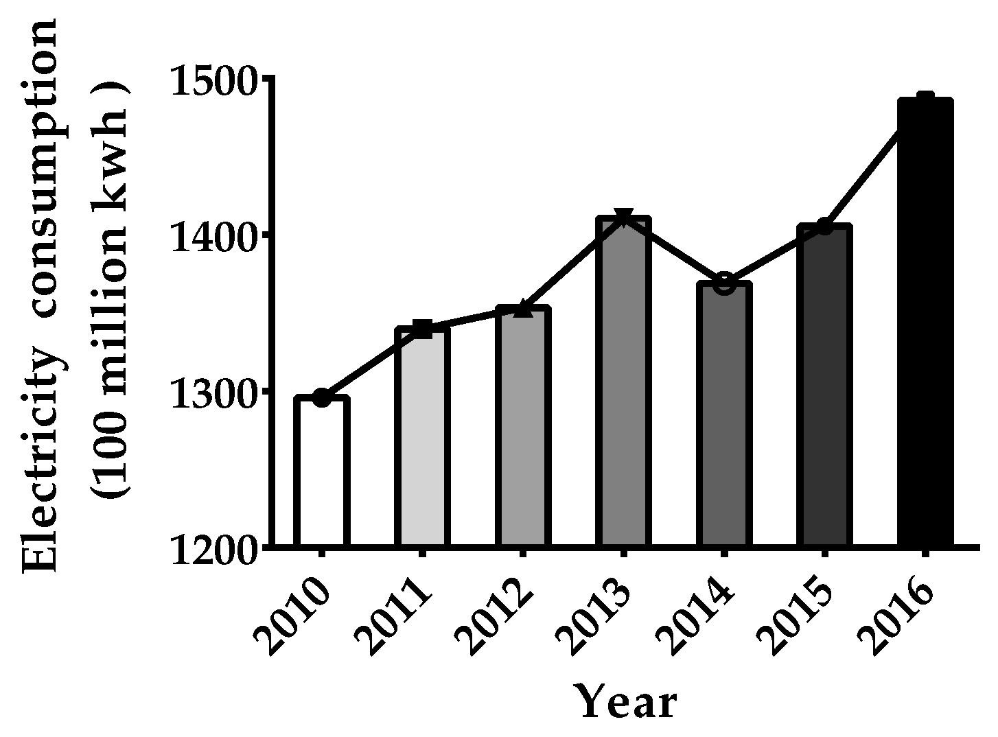
The primitive data sequence of Shanghai’s total electricity consumption in China is collected from the official website of Shanghai City Bureau of Statistics in China (http://www.stats-sh.gov.cn/). The sample data of annual electricity consumption for Shanghai City in China from 2010 to 2016 is listed in Table 4 and illustrated in Figure 2. It can be seen from Figure 2 that Shanghai’s total electricity consumption in China is characteristic of nonlinear growth, and the average increasing speed of electricity consumption in these seven years is about 2.0% per year, although there might be a slight short-term fluctuation.
The detailed procedure to forecast Shanghai’s total electricity consumption is as follows: Firstly, different prediction models, which are DCOGM(1,1), traditional GM(1,1)model, and four published improved GM(1,1)models, DGM(1,1) [51], FGM(1,1) [50], RGM(1,1) [59], TGM(1,1) [54], and linear regression (LR) model, are constructed separately with the data of annual total electricity consumption of Shanghai City from 2010 to 2014, then the prediction performances of those prediction models are examined and compared with the data from year 2015 and 2016, and, finally, the total electricity consumption forecasting of Shanghai city from 2017 to 2021 is predicted by the superior model.

3.3.2. Comparison of the Forecasting Performances of the Predictive Models

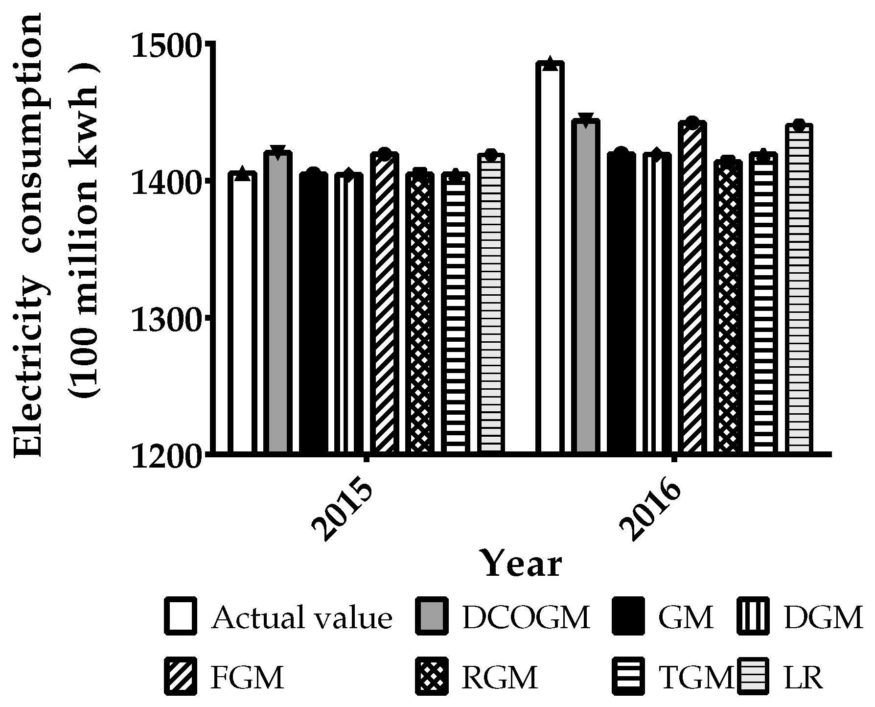
The actual data and predicted data by the seven models for the year 2015 and 2016 are listed in Table 5 and Figure 3. In addition, the most commonly used indices, namely MAPE and RMSE, which are used as the evaluation indices of the forecasting performance for the predictive models, are also listed in Table 5.
As for MAPEs shown in Table 5, it could be concluded that all seven of the predictive models present to be highly accurate ( M A P E < 10 % ) in this study according to Lewis’ benchmark of accuracy evaluation [60]; additionally, DCOGM(1,1) yields the lowest MAPE (1.95%) and bears the highest prediction accuracy, which verifies again that the new proposed model in this study is superior to the other six predictive models.
Finally, according to the RMSE values for the total electricity consumption, which are shown in Table 5, the findings are the same as those for MAPE values above, that is, DCOGM(1,1) has the smallest RMSE and outperforms the other six models in terms of predicting the electricity consumption.
In conclusion, DCOGM(1,1) proposed in this study performs better than the other five grey forecasting models and the LR model. The two evaluation indices confirm that the novel improved grey forecasting model (DCOGM(1,1)) is most suitable for electricity consumption forecasting purposes. Therefore, this novel model will be utilized for forecasting the electricity consumption for Shanghai City in China from 2017 to 2021.

3.3.3. Forecasting the Total Electricity Consumption for Shanghai City in China during 2017–2021

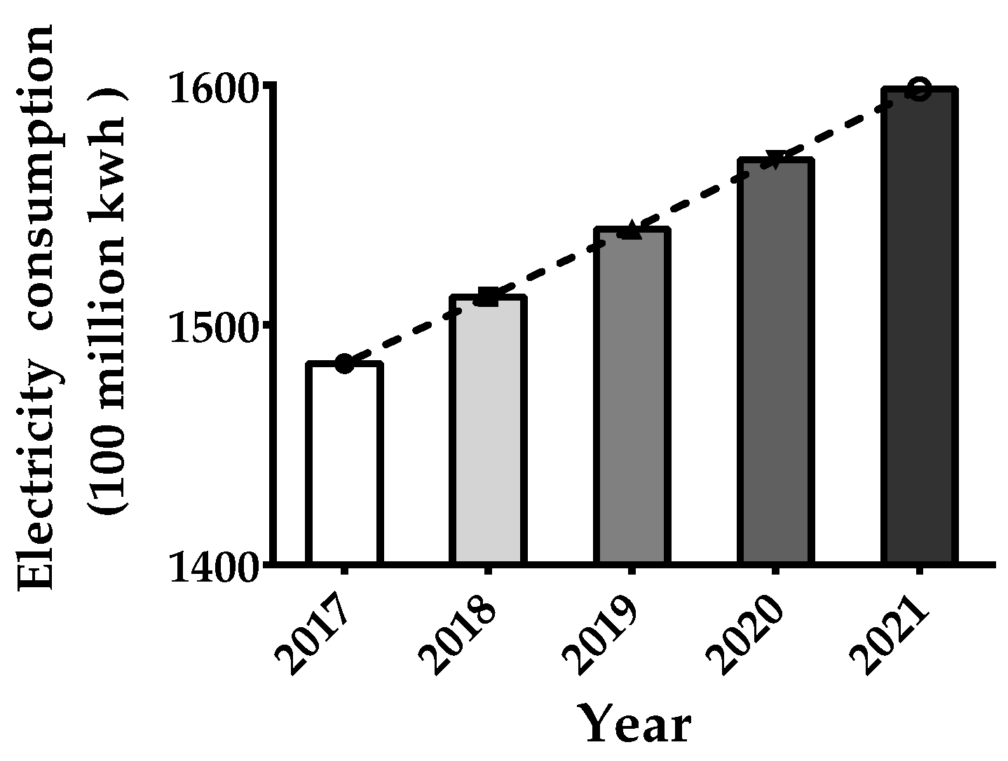
Because of its forecasting accuracy, which is superior to most existing improved GM(1,1) models, DCOGM(1,1) is further applied to predict the electricity consumption for Shanghai City in China from 2017 to 2021. The predicted values are illustrated in Figure 4. It demonstrates that the total electricity consumption for Shanghai City in China will exhibit a relatively stable rising trend in the following five years, and will reach nearly 159.85 billion kwh by the year 2021. In other words, the electricity consumption for Shanghai City in China will increase by nearly 11.25 billion kwh relative to 2016 year by the year of 2021. Under the pressure of an electricity shortage worldwide, it is a huge challenge for Shanghai’s electricity demand strategy, and relevant departments need to make appropriate measures in advance to cope with the looming shortage of electricity demand.

4. Discussion

Prediction of electricity consumption for a country (region) not only plays a significant role in the economy but also is important for policy makers[1]. Accurate prediction results could facilitate effective implementation of electricity supply policies, help avoid economic losses caused by insufficient electricity to a certain extent and reduce operating costs and risks of economy [4]. However, the source database of electricity consumption is often limited with great deviation [29]. Given this, the GM(1,1) model, which is one of the most frequently used grey prediction models and only requires a limited number of samples to construct a prediction model with relatively high prediction accuracy, is an appropriate tool for electricity consumption forecasting.
In this study, we proposed a novel improved GM(1,1) model, DCOGM(1,1), for electricity consumption prediction. To evaluate the simulation and prediction performance of DCOGM(1,1), some compared prediction models, such as statistical analysis models (LR model and MAED [57]), computational intelligence models (BPN, RBFN and SVR), and grey prediction models (AGM(1,1) model [56], GPRM [58], NNGM(1,1) [6], DGM(1,1) [51], FGM(1,1) [50], RGM(1,1) [59], and TGM(1,1) [54]), are selected in this article. From Case 1 and Case 2, we can see that the grey prediction models outperform statistical analysis models and computational intelligence models, that is the MAPEs gained by AGM(1,1) and DCOGM(1,1) are lower than those by BPN and SVR in Case 1 as shown in Table 1 and the MAPEs gained by MAED, BPN and RBFN are higher than those by GPRM, NNGM(1,1) and DCOGM(1,1) in Case 2 as indicated in Table 2. In addition, this could be attributed to limited source data and the distribution of the original data sequence, in the condition of which grey prediction models have more advantages.
The GM(1,1) model is based on the assumption that the original data sequence obeys the exponential distribution [47,61]. However, the practical data sequence often exhibits the characteristic of approximately inhomogeneous exponential growth [48,49]. In addition, the calculation of the background value of GM(1,1) model leads to bias and affects the prediction performance [6,53,54]. Therefore, in this paper, we optimized the GM(1,1) model by combining data transformation for the original data sequence and combination interpolation optimization of the background value, namely DCOGM(1,1). The results of three cases suggest that the prediction performance of DCOGM(1,1) is not only better than statistical analysis models and computational intelligence models, but also better than other grey modification models, such as AGM(1,1) model [56], GPRM [58], NNGM(1,1) [6], DGM(1,1) [51], FGM(1,1) [50], RGM(1,1) [59] and TGM(1,1) [54]. Thus, DCOGM(1,1) is a promising tool for short-term electricity consumption prediction. In addition, combined optimization is a potential method to improve the prediction performance of GM(1,1) model, and could be considered in other circumstances. However, it should be noticed that the performance of long-term forecasting by the DCOGM(1,1) is less efficient than that of short-term forecasting.
Theoretically, grey modification models could improve the prediction accuracy of the GM(1,1) model. However, we can see that the prediction performances of DGM(1,1) [51] and RGM(1,1) [59] are inferior to that of the traditional GM(1,1)model from Case 3 as shown in Table 5. Thus, it is worth noting that grey modification models that can improve the prediction accuracy of the model may not be applied in all situations, since each prediction model has its own scope of application. Thus, caution should be taken before a prediction model is applied in a different context.

5. Conclusions

Accurate prediction of electricity consumption plays an important role in electricity management and economy development. In this paper, we firstly analyze the instinctive characteristics of GM(1,1) model, and find that the distribution of the original data sequence and the background value are two of the most important factors that affect the forecast accuracy of GM(1,1) model, and then we propose a novel improved GM(1,1) model (DCOGM(1,1)), which combines data transformation for the original data sequence and combination interpolation optimization of the background value, to forecast short-term electricity consumption. Two case studies show that DCOGM(1,1) performs better than the traditional GM(1,1) model and some improved GM(1,1) models and has better exploration and exploitation ability. Finally, application of DCOGM(1,1) for total electricity consumption forecasting in Shanghai City not only indicates an increasing electricity consumption demand in the following five years in Shanghai City, but it also verifies the adequate predictive performance of DCOGM(1,1).
Based on the empirical results, we suggest that the DCOGM(1,1), which bears higher prediction precision, could be utilized as an effective and promising forecasting tool in the future. For example, DCOGM(1,1) can be utilized in other forecasting fields, such as GDP forecasting, tourism demand forecasting, peak load forecasting, business forecasting, and natural gas consumption prediction, in the context of which the source data is relatively limited and changes slowly in general.
However, it is worth noting that the prediction accuracy of GM(1,1) model and improved GM(1,1) model may decrease rapidly when the raw data sequence fluctuates dramatically or grows aggressively, thus further improvements will also be needed in such circumstances. Moreover, it is known that the prediction accuracy of the traditional GM(1,1) could be improved by optimization of the initial condition [22] and rolling mechanism [6]. How DCOGM(1,1) can be combined with the optimization of the initial condition and rolling mechanism may be an interesting issue for electricity consumption forecasting. Furthermore, taking advantage of other common techniques to improve the prediction accuracy of the grey prediction model is also meaningful. In addition, all of these issues could be a future focus.

Author Contributions

K.L. designed the structure, performed the calculations and improved the manuscript; T.Z. proposed the idea. Both authors have read and approved the manuscript.

Funding

This work is financially supported by National Natural Science Foundation of China (61572140), the Shanghai Municipal R&D Foundation (17DZ1100504 and 16511104704) and the Graduate Student Innovation Fund Program of Shanghai University of Finance and Economics in 2017 (CXJJ-2017-423).

Acknowledgments

The authors are grateful to editors and anonymous referees for their very valuable comments and suggestions, which have significantly helped improve the quality of this paper.

Conflicts of Interest

No potential conflict of interest was reported by the authors.

References

  1. Xiao, L.; Wang, C.; Liang, T.; Shao, W. A combined model based on multiple seasonal patterns and modified firefly algorithm for electrical load forecasting. Energy Policy 2016, 167, 135–153. [Google Scholar] [CrossRef]
  2. Li, S.; Ma, X.; Yang, C. A novel structure-adaptive intelligent grey forecasting model with full-order time power terms and its application. Comput. Ind. Eng. 2018, 120, 53–67. [Google Scholar] [CrossRef]
  3. Zhao, H.; Guo, S.; Xue, W. Urban saturated power load analysis based on a novel combined forecasting model. Information 2015, 6, 69–88. [Google Scholar] [CrossRef]
  4. Lebotsa, M.E.; Sigauke, C.; Bere, A.; Fildes, R.; Boylan, J.E. Short term electricity demand forecasting using partially linear additive quantile regression with an application to the unit commitment problem. Appl. Energy 2018, 222, 104–118. [Google Scholar] [CrossRef]
  5. Wang, Z.X.; Li, Q.; Pei, L.L. A seasonal GM(1,1) model for forecasting the electricity consumption of the primary economic sectors. Energy 2018, 154, 522–534. [Google Scholar] [CrossRef]
  6. Chung, Y.H. Electricity consumption prediction using a neural-network-based grey forecasting approach. J. Oper. Res. Soc. 2017, 68, 1259–1264. [Google Scholar]
  7. Al-Hamadi, H.M.; Soliman, S.A. Long-term/mid-term electric load forecasting based on short-term correlation and annual growth. Electr. Power Syst. Res. 2005, 74, 353–361. [Google Scholar] [CrossRef]
  8. Pao, H.T. Forecast of electricity consumption and economic growth in Taiwan by state space modeling. Energy 2009, 34, 1779–1791. [Google Scholar] [CrossRef]
  9. Hussain, A.; Rahman, M.; Memon, J.A. Forecasting electricity consumption in Pakistan: The way forward. Energy Policy 2016, 90, 73–80. [Google Scholar] [CrossRef]
  10. Khosravi, A.; Nahavandi, S.; Creighton, D.; Srinivasan, D. Interval type-2 fuzzy logic systems for load forecasting: A comparative study. IEEE Trans. Power Syst. 2012, 27, 1274–1282. [Google Scholar] [CrossRef]
  11. Hernández, L.; Baladrón, C.; Aguiar, J.M.; Calavia, L.; Carro, B.; Sánchez-Esguevillas, A.; García, P.; Lloret, J. Experimental analysis of the input variables’ relevance to forecast next Day’s aggregated electric demand using neural networks. Energies 2013, 6, 2927–2948. [Google Scholar] [CrossRef]
  12. Lee, Y.S.; Tong, L.T. Forecasting energy consumption using a grey model improved by incorporating genetic programming. Energy Convers. Manag. 2011, 52, 147–152. [Google Scholar] [CrossRef]
  13. Červená, M.; Schneider, M. Short-term forecasting of GDP with a DSGE model augmented by monthly indicators. Int. J. Forecast. 2014, 30, 498–516. [Google Scholar] [CrossRef]
  14. Huang, Y.F.; Wang, C.N.; Dang, H.S.; Lai, S.T. Evaluating performance of the DGM(2,1) model and its modified models. Appl. Sci. 2016, 6, 73. [Google Scholar] [CrossRef]
  15. Mohamed, Z.; Bodger, P. Forecasting electricity consumption in New Zealand using economic and demographic variables. Energy 2005, 30, 1833–1843. [Google Scholar] [CrossRef] [Green Version]
  16. Nagbe, K.; Cugliari, J.; Jacques, J. Short-term electricity demand forecasting using a functional state space model. Energies 2018, 11, 1120. [Google Scholar] [CrossRef]
  17. Wang, F.; Wang, F.; Yu, Y.; Wang, X.; Ren, H.; Shafie-Khah, M.; Catalao, J.P.S. Residential electricity consumption level impact factor analysis based on wrapper feature selection and multinomial logistic regression. Energies 2018, 11, 1180. [Google Scholar] [CrossRef]
  18. Cabral, J.D.A.; Legey, L.F.L.; Cabral, M.V.D.F. Electricity consumption forecasting in Brazil: A spatial econometrics approach. Energy 2017, 126, 124–131. [Google Scholar] [CrossRef]
  19. Zhao, W.; Wang, J.; Lu, H. Combining forecasts of electricity consumption in China with time-varying weights updated by a high-order Markov chain model. Omega 2014, 45, 80–91. [Google Scholar] [CrossRef]
  20. Bouzerdoum, M.; Mellit, A.; Pavan, A.M. A hybrid model (SARIMA-SVM) for short-term power forecasting of a small-scale grid-connected photovoltaic plant. Sol. Energy 2013, 98, 226–235. [Google Scholar] [CrossRef]
  21. Al-Hamadi, H.M.; Soliman, S.A. Short-term electric load forecasting based on Kalman filtering algorithm with moving window weather and load model. Electr. Power Syst. Res. 2004, 3, 47–49. [Google Scholar] [CrossRef]
  22. Ding, S.; Hipel, K.W.; Dang, Y.G. Forecasting China’s electricity consumption using a new grey prediction model. Energy 2018, 149, 314–328. [Google Scholar] [CrossRef]
  23. Wu, L.F.; Liu, S.F.; Cui, W.; Liu, D.L.; Yao, T.X. Non-homogenous discrete grey model with fractional-order accumulation. Neural. Comput. Appl. 2014, 25, 1215–1221. [Google Scholar] [CrossRef]
  24. Kaytez, F.; Taplamacioglu, M.C.; Cam, E.; Hardalac, F. Forecasting electricity consumption: A comparison of regression analysis, neural networks and least squares support vector machines. Int. J. Electr. Power 2015, 67, 431–438. [Google Scholar] [CrossRef]
  25. Hu, Y.C.; Jiang, P. Forecasting energy demand using neural-network-based grey residual modification models. J. Oper. Res. Soc. 2017, 68, 556–565. [Google Scholar] [CrossRef]
  26. Cao, G.; Wu, L. Support vector regression with fruit fly optimization algorithm for seasonal electricity consumption forecasting. Energy 2016, 115, 734–745. [Google Scholar] [CrossRef]
  27. Kavousi-Fard, A.; Samet, H.; Marzbani, F. A new hybrid modified firefly algorithm and support vector regression model for accurate short term load forecasting. Expert Syst. Appl. 2014, 41, 6047–6056. [Google Scholar] [CrossRef]
  28. Pozna, C.; Precup, R.E.; Tar, J.K. New results in modelling derived from Bayesian filtering. Knowl. Based Syst. 2010, 23, 182–194. [Google Scholar] [CrossRef]
  29. Xu, N.; Dang, Y.G.; Gong, Y.D. Novel grey prediction model with nonlinear optimized time response method for forecasting of electricity consumption in China. Energy 2017, 118, 473–480. [Google Scholar] [CrossRef]
  30. Deng, J.L. Control problem of grey systems. Syst. Control Lett. 1982, 1, 288–294. [Google Scholar]
  31. Liu, S.; Lin, Y. Grey Information: Theory and Practical Applications; Springer: London, UK, 2006. [Google Scholar]
  32. Talafuse, T.O.; Pohl, E.A. Small sample reliability growth modeling using a grey systems model. Qual. Eng. 2017, 29, 455–467. [Google Scholar] [CrossRef]
  33. Wang, Q.; Liu, L.; Wang, S.; Wang, J.Z.; Liu, M. Predicting Beijing’s tertiary industry with an improved grey model. Appl. Soft. Comput. 2017, 57, 482–494. [Google Scholar] [CrossRef]
  34. Hsin, P.H.; Chen, C.I. Application of trembling-hand perfect equilibrium to Nash nonlinear Grey Bernoulli model: An example of BRIC’s GDP forecasting. Neural. Comput. Appl. 2016, 28, 269–274. [Google Scholar] [CrossRef]
  35. Li, Z.B.; Jiang, Y.; Yue, J.; Zhang, L.; Li, D. An improved gray model for aquaculture water quality prediction. Intell. Autom. Soft Comput. 2012, 18, 557–567. [Google Scholar] [CrossRef]
  36. Wu, L.; Liu, S.; Yao, L.; Xu, R.; Lei, X. Using fractional order accumulation to reduce errors from inverse accumulated generating operator of grey model. Soft. Comput. 2015, 19, 483–488. [Google Scholar] [CrossRef]
  37. Hu, Y.C.; Jiang, P.; Chiu, Y.J.; Tsai, J.F. A novel grey prediction model combining markov chain with functional-link net and its application to foreign tourist forecasting. Information 2017, 8, 126. [Google Scholar] [CrossRef]
  38. Li, G.D.; Masuda, M.; Nagai, M. The prediction for Japan’s domestic and overseas automobile production. Technol. Forecast. Soc. 2014, 87, 224–231. [Google Scholar] [CrossRef]
  39. Chang, C.J.; Yu, L.; Jin, P. A mega-trend-diffusion grey forecasting model for short-term manufacturing demand. J. Oper. Res. Soc. 2016, 67, 1439–1445. [Google Scholar] [CrossRef]
  40. Tang, H.W.V.; Yin, M.S. Forecasting performance of grey prediction for education expenditure and school enrollment. Econ. Educ. Rev. 2012, 31, 452–462. [Google Scholar] [CrossRef]
  41. Chen, Y.Y.; Liu, H.T.; Hsieh, H.L. Time series interval forecast using GM(1,1) and NGBM(1,1) models. Soft. Comput. 2017, 1–15. [Google Scholar] [CrossRef]
  42. Wu, L.; Gao, X.; Xiao, Y.; Yang, Y.; Chen, X. Using a novel multi-variable grey model to forecast the electricity consumption of Shandong Province in China. Energy 2018, 157, 327–335. [Google Scholar] [CrossRef]
  43. Xie, N.M.; Yuan, C.Q.; Yang, Y.J. Forecasting China’s energy demand and self-sufficiency rate by grey forecasting model and Markov model. Int. J. Electr. Power 2015, 66, 1–8. [Google Scholar] [CrossRef]
  44. Zhao, H.; Guo, S. An optimized grey model for annual power load forecasting. Energy 2016, 107, 272–286. [Google Scholar] [CrossRef]
  45. Liang, J.; Liang, Y. Analysis and modeling for China’s electricity demand forecasting based on a new mathematical hybrid method. Information 2017, 8, 33. [Google Scholar] [CrossRef]
  46. Hamzacebi, C.; Es, H.A. Forecasting the annual electricity consumption of Turkey using an optimized grey model. Energy 2014, 70, 165–171. [Google Scholar] [CrossRef]
  47. Zeng, B.; Zhou, M.; Zhang, J. Forecasting the energy consumption of China’s manufacturing using a homologous grey prediction model. Sustainability 2017, 9, 1975. [Google Scholar] [CrossRef]
  48. Zeng, B.; Meng, W.; Tong, M.Y. A self-adaptive intelligence grey predictive model with alterable structure and its application. Eng. Appl. Artif. Intell. 2016, 50, 236–2448. [Google Scholar] [CrossRef]
  49. Xie, N.M.; Liu, S.F.; Yang, Y.J.; Yuan, C.Q. On novel grey forecasting model based on non-homogeneous index sequence. Appl. Math. Model. 2013, 37, 5059–5068. [Google Scholar] [CrossRef]
  50. Tien, T.L. A new grey prediction model FGM(1,1). Math. Comput. Model. 2009, 49, 1416–1426. [Google Scholar] [CrossRef]
  51. Xie, N.M.; Liu, S.F. Discrete grey forecasting model and its optimization. Appl. Math. Model. 2009, 33, 1173–1186. [Google Scholar] [CrossRef]
  52. Deng, J. Introduction to grey system theory. J. Grey Syst. 1989, 1, 1–24. [Google Scholar]
  53. Li, K.; Liu, L.; Zhai, J.; Khoshgoftaar, T.M.; Li, L. The improved grey model based on particle swarm optimization algorithm for time series prediction. Eng. Appl. Artif. Intel. 2016, 55, 285–291. [Google Scholar] [CrossRef]
  54. Hsu, L.C. Using improved grey forecasting models to forecast the output of opto-electronics industry. Expert. Syst. Appl. 2011, 38, 13879–13885. [Google Scholar] [CrossRef]
  55. Turner, P.R. Numerical Integration. In Numerical Analysis; Macmillan College Work Out Series; Palgrave: London, UK, 1994. [Google Scholar]
  56. Li, D.C.; Chang, C.J.; Chen, C.C.; Chen, W.C. Forecasting short-term electricity consumption using the adaptive grey-based approach—Asian case. Omega 2012, 40, 767–773. [Google Scholar] [CrossRef]
  57. Akay, D.; Atak, M. Grey prediction with rolling mechanism for electricity demand forecasting of Turkey. Energy 2007, 32, 1670–1675. [Google Scholar] [CrossRef]
  58. Wang, J.; Jiang, H.; Zhou, Q.; Wu, J.; Qin, S. China’s natural gas production and consumption analysis based on the multicycle Hubbert model and rolling Grey model. Renew. Sustain. Energy Rev. 2016, 53, 1149–1167. [Google Scholar] [CrossRef]
  59. Peng, G.Z.; Wang, H.W.; Song, X.; Zhang, H.M. Intelligent management of coal stockpiles using improved grey spontaneous combustion forecasting models. Energy 2017, 132, 269–279. [Google Scholar] [CrossRef]
  60. Lewis, C. Industrial and Business Forecasting Methods; Butterworth Scientific: London, UK, 1982. [Google Scholar]
  61. Wei, B.; Xie, N.; Hu, A. Optimal solution for novel grey polynomial prediction model. Appl. Math. Model. 2018, 62, 717–727. [Google Scholar] [CrossRef]
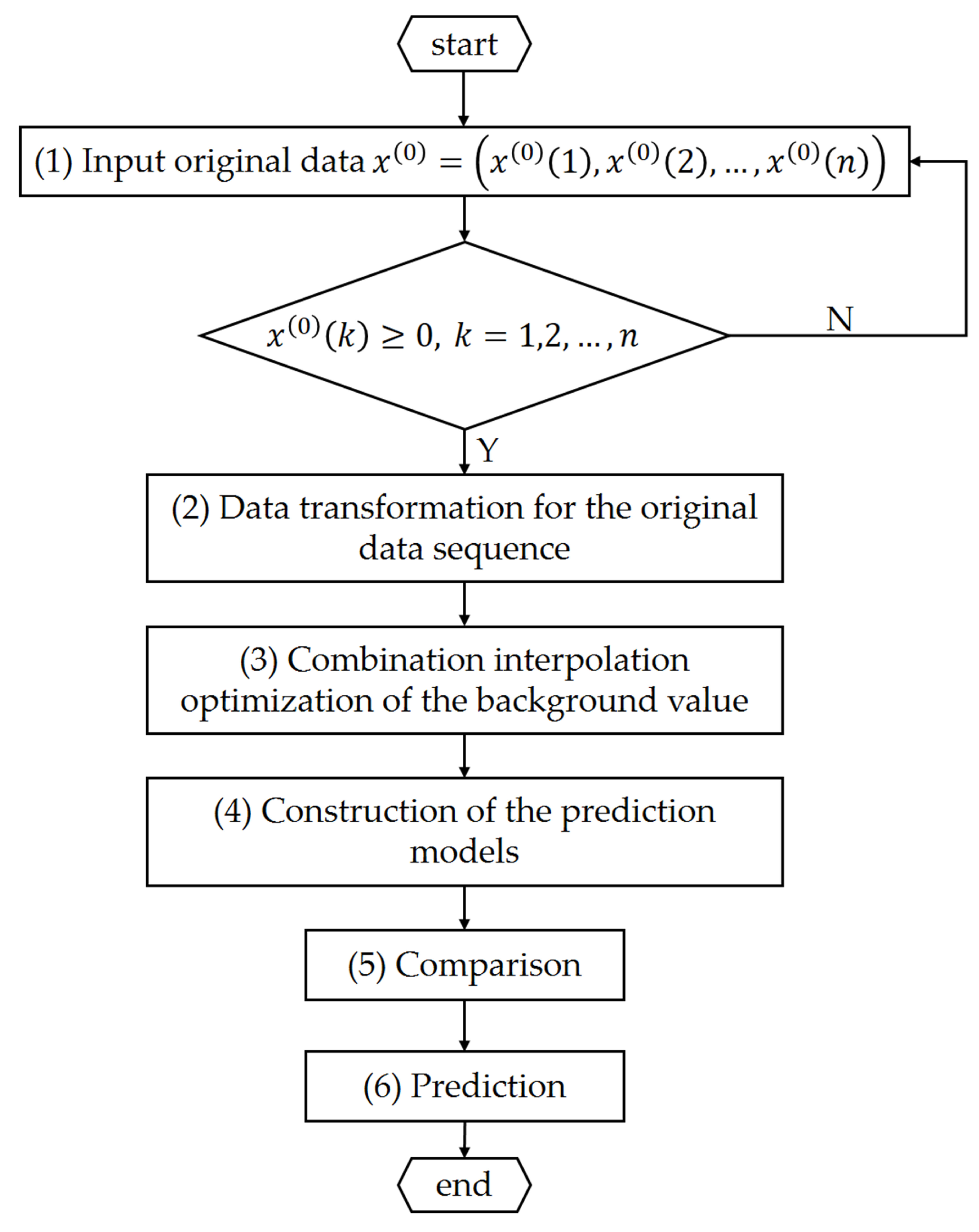
Figure 1. The flowchart of DCOGM(1,1).
Information 09 00204 g001
Figure 2. The electricity consumption for Shanghai City in China from 2010 to 2016.
Information 09 00204 g002
Figure 3. Forecasting results of the electricity consumption.
Information 09 00204 g003
Figure 4. The predictive value of Shanghai’s electricity consumption from 2017 to 2021.
Information 09 00204 g004
Table 1. Absolute percentage error (APE) and MAPE determined by the four compared models for the electricity consumption in APEC.
CoumtryAGM(1,1)BPNSVRDCOGM(1,1)
Australia1.503.026.711.29
Brunei Darussalam6.454.316.222.69
Canada1.861.732.461.33
Chile2.704.7511.402.37
China4.7414.0830.034.43
Chinese Taipei1.104.209.511.15
Hong Kong, China0.571.763.560.64
Indonesia9.587.416.798.44
Japan1.572.113.802.35
Malaysia0.975.1211.721.64
Mexico2.603.608.343.90
New Zealand3.382.826.583.56
Papua New Guinea12.528.237.9311.48
Peru3.987.2613.081.46
Philippines2.373.448.072.53
Russia1.722.725.451.79
Republic of Korea1.125.3912.491.64
Singapore0.963.838.180.64
Thailand0.565.7113.561.55
USA0.961.813.681.55
Vietnam3.7813.7829.741.99
MAPE (%)3.105.109.972.78
Table 2. APE and MAPE obtained by different methods for total electricity consumption.
YearActual Value (TWh)MAEDGPRMBPNRBFNNNGM(1,1)DCOGM(1,1)
199461.408.835.663.162.275.054.35
199567.3910.652.172.583.902.672.97
199674.169.543.804.7215.713.010.74
199781.888.050.594.0115.400.274.55
199887.709.892.760.564.142.945.30
199991.2015.124.862.4711.434.473.16
200098.3016.351.722.5414.982.054.36
200197.0727.336.685.301.315.503.18
2002102.9529.761.461.868.402.553.73
2003111.7729.166.746.309.465.881.97
2004121.1428.781.336.7816.110.870.50
MAPE (%) 17.593.433.669.373.213.17
Table 3. APE and MAPE obtained by different methods for industrial electricity consumption.
YearActual Value (TWh)MAEDGPRMBPNRBFNNNGM(1,1)DCOGM(1,1)
199434.1416.1810.094.460.729.956.83
199538.0117.715.411.9110.255.700.27
199640.6421.312.902.918.201.581.95
199743.4924.762.332.0411.151.784.15
199846.1429.390.770.942.470.725.43
199946.4841.265.845.155.875.691.69
200048.8447.820.880.704.811.491.96
200146.9965.936.277.023.546.656.84
200250.4966.815.054.694.744.324.75
200355.1065.088.398.2310.286.480.34
200459.5764.930.084.997.300.012.52
MAPE (%) 41.934.363.916.304.233.30
Table 4. The electricity consumption for Shanghai City in China from 2010 to 2016 [Unit: 100 million kwh].
Year2010201120122013201420152016
Value1295.871339.621353.451410.611369.021405.561486.02
Table 5. Forecasting results of the electricity consumption for Shanghai City in China by the compared models [Unit: 100 million kwh].
YearDCOGM(1,1)GM(1,1)DGM(1,1)FGM(1,1)RGM(1,1)TGM(1,1)LR
20151420.431404.591404.271419.471404.591404.601418.90
20161443.701419.471419.021442.221413.491419.481440.63
MAPE1.95292.27372.30031.96862.47492.27272.0018
RMSE31.7247.0647.3932.5051.2947.0533.45