Article

Robust Aircraft Detection with a Simple and Efficient Model

1
Institute of Optics and Electronics, Chinese Academy of Sciences, Chengdu 610209, China
2
School of Optoelectronic Science and Engineering, University of Electronic Science and Technology of China, Chengdu 610054, China
3
School of Electronic, Electrical and Communication Engineering, University of Chinese Academy of Sciences, Beijing 100039, China
*
Author to whom correspondence should be addressed.
Information 2018, 9(4), 74; https://doi.org/10.3390/info9040074
Submission received: 28 January 2018 / Revised: 20 March 2018 / Accepted: 22 March 2018 / Published: 29 March 2018
(This article belongs to the Section Information Processes)

Abstract

:
Aircraft detection is the main task of the optoelectronic guiding and monitoring system in airports. In practical applications, we demand not only detection accuracy, but also efficiency. Existing detection approaches always train a set of holistic templates to search over a multi-scale image space, which is inefficient and costly. Moreover, the holistic templates are sensitive to the occluded or truncated object, although they are trained by many complicated features. To address these problems, we firstly propose a kind of local informative feature which combines a local image patch with its corresponding location. Additionally, for computational reasons, a feature compression method (based on sparse representation and compressive sensing) is proposed to reduce the dimensionality of the feature vector, and which shows excellent performance. Thirdly, to improve the detection accuracy during detection stage, a position estimation algorithm is proposed to calibrate the aircraft’s centroid. From the experimental results, our model achieves favorable detection accuracy, especially for the partially-occluded object. Furthermore, the detection speed is remarkably improved as well.

1. Introduction

Object detection is a fundamental task in computer vision. Recently, a large number of detectors have been developed for specific requirements, such as face detection [1], vehicle detection [2], and pedestrian detection [3]. Most of these applications now demand not only accuracy, but also efficiency (fast detection). Aircraft detection is the main task of optoelectronic guiding and monitoring system in airports, which faces many challenges, such as illumination changes, deformation, cluttered scenes, and occlusion. Although many state-of-the-art detection models [3,4,5] achieve favorable performance, they are not suitable to such kinds of systems for two reasons. The first reason is that the models [3,4,5] are time consuming. The second reason is that such models are trained by holistic feature templates, which are sensitive to occlusion. To address these problems, we propose a detection model which combines a local informative patch with a position estimation algorithm for accurate detection. Unlike the detection models trained by a global feature template to detect objects in a sliding window fashion, the proposed local informative feature has two advantages: (a) the local informative feature is robust in detecting partially-occluded objects and (b) the corresponding location adopted in our feature is beneficial for locating the object’s centroid more accurately. By virtue of the local informative feature’s discriminative power, just a simple classifier can yield high performance.
Additionally, higher dimensionality of the feature often leads to higher computational complexity. To improve the efficiency, an approach based on compressive sensing theory is applied in our model. From compressive sensing theory [6,7,8], it is known that if the dimensionality of the feature space is extremely high, these features can be randomly projected to a low-dimensional feature space, which preserves enough information to reconstruct the high-dimensional features. In this paper, we employed the compressed features to train a classifier, which yields favorable detection accuracy as well as fast detection speed. Figure 1 shows the framework of the proposed model, which illustrates two stages: the training stage and the testing stage. In the training stage, a feature dictionary with a local informative patch is built firstly, and then a very sparse matrix is constructed to map the high-dimensional features into the low-dimensional domain. Lastly, a gentle Ada-boost classifier is trained by the compressed features. In the testing phase, we adopt the same method to compress the features and put the low-dimensional features into the trained classifier for classification. The contributions of this paper are:
  • To deal with the practical problems, we designed an efficient model for the specific-category (aircraft) detector, and this model is different from the traditional detection model which detects objects with a holistic feature template in a sliding window fashion.
  • We proposed a local informative feature and built an informative feature dictionary. In addition, a position estimation algorithm was proposed to search the optimal object’s centroid. Experimental results present the discriminative power of this kind of feature, especially for the partially-occluded objects.
  • A compressed method based on compressive sensing and sparse representation was proposed to reduce the computational complexity. From the experimental results, the compressed method achieved high detection accuracy and decreased time consumption.
The rest of this paper is organized as follows: In Section 2, we introduce the relevant studies about aircraft detection and related technologies. In Section 3, the basic theories and analysis regarding feature extraction and compressive sensing are presented and introduced. The detailed implementation of our model is described in Section 4. In Section 5, experimental results and analysis are presented. We conclude this paper and propose future work in the Section 6.

2. Related Work

In this section, we briefly review the recent aircraft detection models [9,10,11] and the related technologies [3,4,5,12,13,14,15,16,17,18,19,20,21] in the literature on object detection.
Compared with other detection task, such as lane detection [22], license plate detection [23], and face detection [1], aircraft detection faces more challenging problems, like various weather conditions, occlusion, cluttered scenes, and illumination changes. In addition, our system requires fast detection speed which significantly supports the aircraft tracking and guidance. Recently, a great many aircraft detection models have been designed. Wu et al. [9] proposed a detection model which applied a similarity measure for aircraft type recognition. However, this model is not suitable for the aircraft in cluttered scenes and varied postures. Rastegar et al. [10] proposed a model which combined wavelets with SVM, and it was applied to detect the aircraft in the original video and images. However, the procedure of training is time-consuming. Liu et al. [11] proposed an efficient approach for feature extraction in high-resolution optical remote sensing images. A rotation invariant feature combined sparse coding and radial gradient transform was presented and showed high performance. However, this model is inefficient for our images obtained from optoelectronic cameras.
In the last decade, object detection technologies have achieved great success. Dalal et al. [3] proposed a discriminative detection model which combined linear SVM with HOG (histogram of oriented gradient) and obtained great success in pedestrian detection. Due to its discriminative power, the HOG feature was adopted widely in object detection. Felzenszwalb et al. [4] proposed a detection model based on a mixture of multiscale deformable part models and made further improvement on original HOG feature. Although it obtained favorable performance on detection accuracy (especially for the object with pose changing), it is costly. These kinds of models always search for an image pyramid space and match the location of the object. Once the objects were occluded partially, or truncated, it was difficult to detect. Malisiewicz et al. [5] discard the partial models in [4] and trained a model called exemplar-SVMs, which included a set of holistic templates (exemplars) for a specific category and which handled the inner-categories detection problem (objects in one specific category have great differences) and accelerated the detection. However, it was still based on a sliding window fashion. With the increase of exemplars, the computational cost grew as well. In order to speed up detection, Song et al. [18,19,20] improved the DPM models [4] and proposed the sparselet models which use the shared intermediate representations and reconstruction sparsity to accelerate the multi-class object detection. The sparselet models not only achieve the favorable accuracy, but also reduce the time cost greatly. Cheng et al. [21] improved the previous work and proposed coarse-to-fine sparselets, which combines coarse and fine sparselets and outperforms the sparselets baseline work.
Moreover, some works were proposed to reduce the searching space by extracting the candidate regions. The works [13,14] proposed the rough segmentation method to reduce the search spaces for category-specific detectors. However, these methods are still computationally expensive, and which cost minutes per image. Uijlings et al. [12] proposed a method named selective search which generates several candidate regions for detecting, and the number of candidate regions is much less than the searching space of the sliding window method. However, the detection results are object-like things rather than category-specific objects. Therefore, several category-specific detectors [15,16] were developed based on this method; however, the hierarchies of these detectors are complicated.
In all cases, occlusions always cause a significant decrease in performance. Actually, the above studies have not focused on such problems. Shu et al. [24] proposed a part-based model for pedestrian detection. Tian et al. [25] also applied part information to detect vehicles. These models always handle the part information of a specific object before training.
Therefore, the consideration of our work refers to two aspects: (1) developing an efficient and accurate aircraft detection model; and (2) this model is robust for partially occlusion.

3. Methods

3.1. Informative Features

In many computer vision systems, the informative features are specific image patches extracted from images based on local image properties [26] or eigen-patches [27] of similar parts. These selected features represent the maximal information to the corresponding class. Ullman et al. [28] employed such informative feature to train a simple linear classifier, and which outperformed the generic type features, such as wavelets. Leibe et al. [29] combined informative patterns with spatial information and trained a discriminative classifier.
We were enlightened by these works and designed a combined feature which includes an image patch as well as its location information. The local informative feature is formed as <pf, lf>, where, the pf represents the extracted patch, and lf is represented by two sparse vectors (lfx, lfy) which are corresponding to the object’s centroid. Unlike the local pattern and spatial location distribution presented in [29], our proposed sparse vector is easy to implement. In Figure 2, the green and red patches are informative patches, and the red one is the centroid of the object; lf is computed by Equations (1) and (2):
{ d x = 2 × | p x c x | + 1 , d y = 2 × | p y c y | + 1
l f x ( i ) = { 1 ,   i = ( d x + 1 ) / 2 ( p x c x ) 0 ,   o t h e r s l f y ( i ) = { 1 ,   i = ( d y + 1 ) / 2 ( p y c y ) 0 ,   o t h e r s
where (px, py) is the central coordinate of the patch, (cx, cy) is the position of object’s centroid, (dx, dy) represent the length of (lfx, lfy), and i represents the ith entry of the vector.

3.2. Informative Feature Dictionary

Unlike the works [26,27,28,29,30] that adopted a random sampling method to extract the informative patch pf, we proposed another way to extracted more informative features <pf, lf>. For each image, the informative feature extraction process is described in Table 1 and Figure 3:
Actually, the elements in the informative feature dictionary include rich edge information, which are discriminative for detection. Figure 3 illustrates some informative patches with rich edge information.

3.3. Random Projection

Random projection [32] refers to mapping a high-dimensionality dataset into a lower dimensionality space, which provides some guarantees on the approximate preservation of distance. Now, suppose that we have a vector u in the high dimensionality feature space, u m , a vector v in the low dimensionality space, v n , a random matrix A n × m , the mapping as Equation (3):
v = A × u
where n < < m . Each projection v is essentially equivalent to a compressive measurement in the compressive sensing encoding stage [33]. From the compressive sensing theory, if a signal is a linear combination of only K basis [34], the signal can be reconstructed from a small number of random measurements. Therefore, it is essentially to identify an effective random matrix for feature extraction.
Ideally, we expect to ensure that A is information preserving, by which we mean that A provides a stable embedding which approximately preserves distances between each pairs of all signals [35]. Therefore, for every two feature vectors (e.g., u k , u l , k l ) in our method, their distance is approximately preserved. For the feature vectors u 1 , u 2 :
1 ε A * u 1 A * u 2 l 2 2 u 1 u 2 l 2 2 1 + ε
In Equation (4), ε is a small value, and ε > 0 . One important result in the compressive theory [6] named RIP (restricted isometry property) reveals that Equation (4) is satisfied with high probability by certain random matrices. Furthermore, the above result is also directly obtained from the JL (Johnson-Lindenstrauss) lemma [34], which also provides us strong theoretical support for reducing feature vectors by random matrix.
Baraniuk et al. [36] proved that the random matrix satisfied with JL lemma holds true for RIP as well. Therefore, the feature vector u can be reconstructed from low-dimensional vector v with minimum error and high probability.

3.4. Sparse Random Measurement Matrix

Liu et al. [35] employed the random Gaussian matrix A n × m where A ( i , j ) = a i j , and a i j N ( 0 , 1 ) (i.e., zero mean and unit variance), the results showed that sparse random measurement matrix for texture classification is favorable. However, the random Gaussian matrix is still dense (which leads to more computational loads). We define a very sparse measurement matrix with sparse elements as below:
a i j = s × { 1 , with   probability   1 / ( 2 s ) 0 , with   probability   1 1 / s 1 , with   probability   1 / ( 2 s )
Achlioptas [31] proved that when s = 1 or s = 3, the matrix would meet the JL lemma. If s = 3, two thirds of the computation load will be reduced. Moreover, Li et al. [37] proved that one can use s > > 3 , e.g., s = m , or even s = m log 10 m , and the results presented that a very sparse matrix obtained the equivalent performance as the former Gaussian matrix. The random matrix in Equation (5) asymptotically satisfies the JL lemma with such s: s = m , s = m log 10 m . In our work, we defined s = m log 10 m to create a very sparse measurement matrix.

4. Proposed Model

The training stage is divided into the following steps: building feature dictionary, forming training samples, compressing features, and building classifier. In the detection stage, a position estimation method is proposed to calibrate the aircraft’s centroid.

4.1. Feature Dictionary

Training images were divided into two subsets. One was employed to build a feature dictionary, and another was applied to generate training samples. Forty images were adopted for establishing the informative feature dictionary. At first, we normalized the object in training images into a fixed scale, such as 40 × 120 pixels, and then extracting the informative patches following the process in Figure 3 and Table 1. For each image, about 800 candidate patches (of size 15 × 15 pixels) were extracted, and then we adopt the NMS algorithm to eliminate the overlapped candidate patches. The rest candidate informative patches were clustered by k-means. We set the parameter K = 40. Finally, 1600 informative patches were extracted and the corresponding locations were calculated by Equation (1) and (2) simultaneously.

4.2. Training Samples

When the feature dictionary was built, like [30], we performed the steps in Table 2 for collecting positive and negative samples.
From the steps in Table 2, the dimensionality of the feature vector was exactly equivalent to the size of the feature dictionary. Therefore, a 1600 D (D is short for dimensionality) feature vector was computed (from step 3 to step 5), and this was described by Equation (6):
v f ( x , y , σ ) = ( | I σ p f | p * l f )
where v f ( x , y , σ ) is the feature vector at position (x, y), σ is the scale of image, pf and lf are defined in Equations (1) and (2), represents normalized cross correlation, and * represents 2-D convolution. In addition, we performed element-wise exponentiation in step 3, which has the effect of prompting template matching. Figure 4 illustrates an example of computing feature vector at each location. We adopted a local informative patch to compute the feature vector and, from the result (the right column of Figure 4), there is a higher response at the center of the object. According to the method in Table 2, a 1600 D feature vector is generated at each position (x, y). For each training images, 40 background points were randomly extracted as negative samples and the object’s centroid was selected as positive samples.
During the detection stage, objects are detected by adopting the classifier to the set of feature vectors at each position of an image.

4.3. Features Compression

To reduce the computational complexity, we employed a very sparse measurement matrix (Section 3.4) for feature compression. Assume that the extracted feature vector was u, where, u m . We defined a very sparse matrix A n × m as Section 3 introduced. With only a multiplication operation, the compressed feature v ( v n ) was obtained. Figure 5 illustrates the process of feature extraction and classification. The feature vectors filled with red points and green points represent positive and negative samples, respectively.

4.4. Classification Algorithm

In this paper, we adopted the gentle Ada-Boost for classification, which is one of the most important classification methodologies in the boosting algorithm family [38]. This algorithm is widely used in object detection and classification [39,40,41]. The boosting algorithm is a formation of additive models like Equation (7):
H ( x ) = n = 1 N h n ( x )
where x is the input feature vector, N is the number of boosting rounds, hn (x) are called weak learners, and H (x) is the strong learner. The principle of the boosting algorithm is that the combinations of weak learners will produce a powerful classification ability. More details of this algorithm can be seen in [38]. Additionally, it is easy to analyze that the training time of this classifier depends on the training rounds.

4.5. Position Estimation

For a testing image, each position was computed by Equation 6 and quantized into a feature vector. This feature vector was compressed and then scored by the trained Ada-Boost model. Therefore, the output of the classifier is a score map which has the equivalent size of testing image. The position in the score map with greater response has a higher probability to be the object’s centroid. In order to calibrate the position of the object’s centroid, a position estimation algorithm (Algorithm 1) was proposed.
Algorithm 1. Position estimation for a score map (from the classifier).
Input: Sw*h (Score map from classifier)
Output: P (position of object’s centroid)
Initialize: P = ¢
Calculating regional maxima of score map: P = {pi |pi = (xi, yi, si)},i = 1…M
Calculating Euclid distance d (pj, pk) of each pair of regional maxima in P:
While min (d (pj, pk)) < θ
 calculating new position and updating the score: pnew = (xnew, ynew, snew)
 updating P: P = (PU{pnew})\{pj, pk}
 updating d (pj, pk)
end while
return P
In Algorithm 1, Sw*h is a score map (in Figure 6a) calculated by classifier, and the regional maxima (in Figure 6c) is represented by pi = (xi, yi, si) where,(xi, yi) and si represent the position and regional maxima score, respectively, and θ was defined as a threshold. We think that two closer regional maxima lead to false positives. Therefore, we employed Equations (8) and (9) to calculate a new position to replace the two closer points. The position with greater value contributes more weights for the generated new position. Figure 6 illustrates an example of the position estimation.
w = [ w j w k ] = [ s j s j + s k s k s j + s k ] , x = [ x j , x k ]   a n d   y = [ y j , y k ]
x n e w = w , x ,   y n e w = w , y , s n e w = w , s

5. Experiment and Results

To validate the performance of the proposed model, we evaluated it on two datasets: the moving aircraft database and the Caltech 101 dataset [2]. All methods in this experiment were programmed in Matlab 2012b and all experiments were run on a PC with an Intel Core i5 CPU (2.5 GHz) and 10 GB memory.

5.1. Moving Aircraft Database

We created a database, named the moving aircraft database, for validation. This database includes about 2500 aircraft images sampled from 19 moving aircraft video series that were obtained by our optoelectronic camera. The captured aircrafts in the images show various appearances and postures in different backgrounds (in Figure 7). In the experiments, features with the fixed size of 1600 D were extracted based on the method in Section 4. Afterwards, they were compressed to 100 D for training and testing.
We compared our model with other two state-of-the-art models: Deformable Parts Model (DPM) [4] and exemplar-SVMs [5]. The performance was considered from two aspects: detection accuracy and detection time. The detection accuracy was evaluated by the average precision: when the overlap ratio (between a detected region and ground truth) is greater than 0.5 it will be defined as true, otherwise, it is false. Four detectors (the gentle Ada-Boost model with various numbers of weak learners, N = 50, 100, 150, 200) were trained for testing. Additionally, we trained a DPM model with six components based on [4] and an exemplar-SVMs model with 300 exemplars like [5]. From the experimental results in Figure 8, our detectors achieved comparable detection accuracy with the DPM and outperformed the exemplar-SVMs.
Furthermore, we tested these three kinds of detectors on the images with partially occluded aircrafts. In this case, our detector (which includes N = 200 weak learners) obtained best performance (in Table 3). Actually, the DPM and exemplar-SVMs adopted holistic templates to match objects in the image pyramid with a slide window fashion. Once the object was occluded, it would obtain a lower matching score, which causes undetected error or mismatch. However, the local informative patch is much smaller than the holistic template, which reduces the chance of mismatch for partial occlusion. An existing drawback of the local feature is a lack of spatial information; therefore, our local informative feature incorporates location information. Figure 9a illustrates some detection examples of partially-occluded aircrafts, and Figure 9b shows the detection results of the aircrafts with different parts occluded.

5.2. Caltech 101 Database

The Caltech 101 database is a popular benchmark database in computer vision. This database contains from 31 to 1100 images per category. We selected about 1074 images from the sub-category of aircraft for training and testing. Most images are medium resolution with the size of 500 × 800. The methods in [4,5] were adopted for comparison. About 200 images were selected for testing. Additionally, we manually occluded the different parts of aircrafts in these images for occlusion testing. From the results showed in Table 4, the exemplar-SVMs obtained the best detection accuracy on original images. However, for the occluded images, our detector outperformed it.
Moreover, we evaluated the per image detection time of each detector. We evaluated 100 images and obtained the average time. From Table 5, for a testing image with the size of 500 × 800 pixels, the detection time of our detector is much less than the detectors based on [4,5].

5.3. Analysis of Feature Compression

5.3.1. Detection Accuracy

In order to validate the performance of the compressed features, a subset of moving aircraft database was selected for testing. We compressed the 1600 D original feature by three methods: principal components analysis (PCA), singular value decomposition (SVD), and our method.
PCA [42,43] and SVD [44] are widely used in dimensionality reduction, which map signals from a high-dimensional space to a low-dimensional space. This mapping always preserves principal information of signal; the noise and contribute-less information was discarded. For the same training set, we employed PCA and SVD, respectively. Figure 10 illustrates the information preservation percentage of each method. For the same training set, 100 D features preserved 96.4% information of PCA, and 95.2% of SVD. We constructed a sparse matrix of size 100 × 1600 by the method in Section 3.4. Detectors were trained by three kinds of compressed features and uncompressed features, and the detection results are shown in Figure 11.
From Figure 11, our compressed features obtained the comparable performance with the uncompressed features, and our method outperformed others. Figure 12 illustrates the relationship between compressed dimensionality and detection accuracy. Our method shows an obvious improvement at the lower dimensionality, which performs better than other two.

5.3.2. Computational Complexity Analysis

For PCA, the process of eigenvalue decomposition is essential. The data is projected onto a subspace by multiplying important eigenvectors (the first k principal components) in Equation (10):
X p r o j e c t i o n = X E k
where X m × n is the original data, E k n × k contains the k eigenvectors corresponding to the k largest eigenvalues. However, the eigenvalue decomposition of the data covariance matrix (of size n × n for n-dimensional data) is time consuming. The computational complexity of PCA is estimated as O (n2m) [42], where m > n. For SVD, the decomposition process aims to obtain the k largest singular value instead of eigenvalue, and its projection follows Equation (10) as well. Therefore, its computational complexity is equivalent to PCA.
The computational process of our method is very simple: the computational complexity of constructing the random matrix A is of order O(mn). We compared the time consumption (which incorporates matrix construction time and feature multiplication time) of these three methods. The feature vectors were compressed from 1600 D to 800 D, 400 D, 200 D, 100 D, and the results are shown in Table 6. The time consumption is average time of 10-fold tests, and our method costs much less than the other two methods.

5.3.3. Model Construction Time

For fast detection system, the detection model usually updates frequently. The consideration of reducing the classifier construction time and detection time is significant. Detection time is always depended on classifier. For the Ada-Boost algorithm, dimensionality of feature vectors yield less impact on the detection time. Therefore, we focused more on decreasing the classifier construction time. It is easy to analyze that the dimensionality of features and numbers of weak learners are two factors.
In our experiments, we employed compressed and uncompressed features to train the classifier. Figure 13 illustrates the training time of a set detectors (with various weak learners). The training time of 1600 D uncompressed features and 100 D compressed features are displayed. Time consumption of the compressed features (our method and PCA) are little different, which is much less than the uncompressed features consumed. For example, in Figure 13, we trained a detector (200 weak learners) with compressed and uncompressed features, the training time are 2.74 s and 26.53, respectively. When the number of weak learners increases, the gap becomes larger and larger. Therefore, training detector with compressed features is an efficient method which not only guarantees high accuracy, but also consumes less time.

6. Conclusions

In this paper, we proposed an aircraft detection model to deal with the practical problem in our optoelectronic guiding and monitoring system, and which is robust in cluttered and partial-occlusion scenes. Firstly, we proposed a local informative feature and built an informative feature dictionary. With the employment of location information, the proposed feature is efficient for locating the object’s centroid. In addition, a position estimation algorithm is proposed for further optimization at the detection stage. For computational reasons, a simple and efficient compression approach was designed for feature compression. Unlike the traditional compression methods requiring complicated matrix decomposition, we just employed a very sparse matrix to reduce the feature dimensionality. From the experimental results, our proposed model achieved favorable accuracy and speed.
Our future work will focus on two aspects: developing more powerful features and improving the positioning accuracy of objects. In this work, only the simple local feature yields excellent results, and we think there is room for improvement. Moreover, the positioning of small objects is still challenging; if the positioning accuracy increases, the detection accuracy will be improved. Finally, applying this model to other specific categories (such as vehicle or pedestrian) is very interesting as well.

Acknowledgments

This work was supported by Youth Innovation Promotion Association, CAS (Grant No. 2016336). The authors would appreciate the anonymous reviewers for their valuable comments and suggestions for improving this paper.

Author Contributions

J.Z. proposed the original idea and wrote this paper; T.L. gave many valuable suggestions and revised the paper; and G.Y. and P.J. designed a part of the experiments and revised the paper.

Conflicts of Interest

The authors declare no conflict of interest.

References

  1. Viola, P.; Jones, M. Robust real-time object detection. Comput. Vis. 2004, 57, 137–154. [Google Scholar] [CrossRef]
  2. Li, F.; Fergus, R.; Perona, P. Learning generative visual models from few training examples: An incremental Bayesian approach tested on 101 object categories. In Proceedings of the IEEE Conference on Computer Vision and Pattern Recognition, Washington, DC, USA, 27 July–2 June 2004; pp. 178–189. [Google Scholar]
  3. Dalal, N.; Triggs, B. Histograms of oriented gradients for human detection. In Proceedings of the IEEE Conference on Computer Vision and Pattern Recognition, San Diego, CA, USA, 20–25 June 2005; pp. 886–893. [Google Scholar]
  4. Felzenszwalb, P.; Girshick, R.; McAllester, D.; Ramanan, D. Object detection with discriminatively trained part based models. IEEE Trans. Pattern Anal. Mach. Intell. 2010, 32, 1627–1645. [Google Scholar] [CrossRef] [PubMed]
  5. Malisiewicz, T.; Gupta, A.; Efros, A.A. Ensemble of exemplar-SVMs for object detection and beyond. In Proceedings of the International Conference on Computer Vision, Barcelona, Spain, 6–13 November 2011; pp. 89–96. [Google Scholar]
  6. Baraniuk, R. Compressive sensing. IEEE Signal Process. Mag. 2007, 24, 118–121. [Google Scholar] [CrossRef]
  7. Candes, E.; Tao, T. Near-optimal signal recovery from random projections: Universal encoding strategies? IEEE Trans. Inf. Theory 2006, 52, 5406–5425. [Google Scholar] [CrossRef]
  8. Donoho, D. Compressed sensing. IEEE Trans. Inf. Theory 2006, 52, 1289–1306. [Google Scholar] [CrossRef]
  9. Wu, Q.; Sun, H.; Sun, X.; Zhang, D.; Fu, K.; Wang, H. Aircraft Recognition in High Resolution Optical Satellite Remote Sensing Images. IEEE Geosci. Remote Sens. Lett. 2015, 12, 112–116. [Google Scholar]
  10. Rastegar, S.; Babaeian, A.; Bandarabadi, M.; Toopchi, Y. Airplane Detection and Tracking Using Wavelet Features and SVM Classifier. In Proceedings of the 41st Southeastern Symposium on System Theory, Tullahoma, TN, USA, 15–17 March 2009; pp. 64–67. [Google Scholar]
  11. Liu, L.; Shi, Z. Airplane detection based on rotation invariant and sparse coding in remote sensing images. Optik 2014, 125, 5327–5333. [Google Scholar] [CrossRef]
  12. Uijlings, J.; Van de Sande, K.; Gevers, T.; Smeulders, A. Selective search for object recognition. Int. J. Comput. Vis. 2013, 104, 154–171. [Google Scholar] [CrossRef]
  13. Carreira, J.; Sminchisescu, C. CPMC: Automatic object segmentation using constrained parametric min-cuts. IEEE Trans. Pattern Anal. Mach. Intell. 2012, 34, 1312–1328. [Google Scholar] [CrossRef] [PubMed]
  14. Endres, I.; Hoiem, D. Category independent object proposals. In Proceedings of the 11th European Conference on Computer Vision, Heraklion, Crete, Greece, 5–11 September 2010; pp. 575–588. [Google Scholar]
  15. Girshick, R.; Donahue, J.; Darrell, T.; Malik, J. Rich feature hierarchies for accurate object detection and semantic segmentation. In Proceedings of the IEEE Conference on Computer Vision and Pattern Recognition, Columbus, OH, USA, 23–28 June 2014; pp. 580–587. [Google Scholar]
  16. Wang, C.; Ren, W.; Huang, K.; Tan, T. Weakly Supervised Object Localization with Latent Category Learning. In Proceedings of the 13th European Conference on Computer Vision, Zurich, Switzerland, 6–12 September 2014; pp. 431–445. [Google Scholar]
  17. Lin, Y.; Liu, T.; Fuh, C. Fast Object Detection with Occlusions. In Proceedings of the 8th European Conference on Computer Vision, Prague, Czech Republic, 11–14 May 2004; pp. 402–413. [Google Scholar]
  18. Song, H.; Girshick, R.; Zickler, S.; Geyer, C. Generalized Sparselet Models for Real-Time Multiclass Object Recognition. IEEE Trans. Pattern Anal. Mach. Intell. 2015, 37, 1001–1012. [Google Scholar] [CrossRef] [PubMed]
  19. Song, H.; Zickler, S.; Althoff, T.; Girshick, R.; Fritz, M.; Geyer, C.; Felzenszwalb, P.; Darrell, T. Sparselet models for efficient multiclass object detection. In Proceedings of the European conference on Computer Vision, Florence, Italy, 7–13 October 2012; pp. 802–815. [Google Scholar]
  20. Girshick, R.; Song, H.; Darrell, T. Discriminatively activated sparselets. In Proceedings of the 30th International Conference on International Conference on Machine Learning, Atlanta, GA, USA, 16–21 June 2013; pp. 196–204. [Google Scholar]
  21. Cheng, G.; Han, J.; Lei, G.; Liu, T. Learning coarse-to-fine sparselets for efficient object detection and scene classification. In Proceedings of the IEEE Conference Computer Vision and Pattern Recognition, Boston, MA, USA, 7–12 June 2015; pp. 1173–1181. [Google Scholar]
  22. You, F.; Zhang, R.; Zhong, L.; Wang, H.; Xu, J. Lane Detection Algorithm for Night-time Digital Image Based on Distribution Feature of Boundary Pixels. J. Opt. Soc. Korea 2013, 17, 188–199. [Google Scholar] [CrossRef]
  23. Lee, D.; Choi, J. Precise Detection of Car License Plates by Locating Main Characters. J. Opt. Soc. Korea 2010, 14, 376–382. [Google Scholar] [CrossRef]
  24. Shu, G.; Dehghan, A.; Oreifej, O.; Hand, E.; Shah, M. Part-based Multiple-Person Tracking with Partial Occlusion Handling. In Proceedings of the 8th European Conference on Computer Vision, Providence, RI, USA, 16–21 June 2012; pp. 1815–1821. [Google Scholar]
  25. Tian, B.; Tang, M.; Wang, F. Vehicle detection grammars with partial occlusion handling for traffic surveillance. Transp. Res. Part C Emerg. Technol. 2015, 56, 80–93. [Google Scholar] [CrossRef]
  26. Agarwal, S.; Roth, D. Learning a sparse representation for object detection. In Proceedings of the 7th European Conference on Computer Vision, Copenhagen, Denmark, 28–31 May 2002; pp. 113–130. [Google Scholar]
  27. Weber, M.; Welling, M.; Perona, P. Unsupervised learning of models for recognition. In Proceedings of the 6th European Conference on Computer Vision, Dublin, Ireland, 28 June–1 July 2000; pp. 18–32. [Google Scholar]
  28. Vidal-Naquet, M.; Ullman, S. Object Recognition with Informative Features and Linear Classification. In Proceedings of the IEEE International Conference on Computer Vision, Nice, France, 13–16 October 2003; pp. 281–289. [Google Scholar]
  29. Leibe, B.; Leonardis, A. Schiele, B. An Implicit Shape Model for Combined Object Categorization and Segmentation. Lect. Notes Comput. Sci. 2006, 4170, 508–524. [Google Scholar]
  30. Torralba, A.; Murphy, K.P.; Freeman, W.T. Sharing Visual Features for Multiclass and Multiview Object Detection. IEEE Trans. Pattern Anal. Mach. Intell. 2007, 29, 854–869. [Google Scholar] [CrossRef] [PubMed]
  31. Neubeck, A.; Van Gool, L. Efficient Non-Maximum Suppression. In Proceedings of the International Conference on Pattern Recognition, Hong Kong, China, 20–24 August 2006; pp. 850–855. [Google Scholar]
  32. Achlioptas, D. Database-friendly random projections: Johnson-Lindenstrauss with binary coins. J. Comput. Syst. Sci. 2003, 66, 671–687. [Google Scholar] [CrossRef]
  33. Zhang, K.; Zhang, L.; Yang, M. Real-time Compressive Tracking. In Proceedings of the 12th European Conference on Computer Vision, Florence, Italy, 7–13 October 2012; pp. 864–877. [Google Scholar]
  34. Dasgupta, S.; Gupta, A. An Elementary Proof of a Theorem of Johnson and Lindenstrauss. Random Struct. Algorithms 2003, 22, 60–65. [Google Scholar] [CrossRef]
  35. Liu, L.; Fieguth, P. Texture Classification from Random Features. IEEE Trans. Pattern Anal. Mach. Learn. 2012, 34, 574–586. [Google Scholar] [CrossRef] [PubMed]
  36. Baraniuk, R.; Davenport, M.; DeVore, R.; Wakin, M. A simple proof of the restricted isometry property for random matrices. Constr. Approx. 2008, 28, 253–263. [Google Scholar] [CrossRef]
  37. Li, P.; Hastie, T.; Church, K. Very sparse random projections. In Proceedings of the International Conference on Knowledge Discovery and Data Mining, Philadelphia, PA, USA, 20–23 August 2006; pp. 287–296. [Google Scholar]
  38. Friedman, J.; Hastie, T.; Tibshirani, R. Additive logistic regression: A statistical view of boosting. Ann. Stat. 2000, 28, 337–374. [Google Scholar] [CrossRef]
  39. Mei, K.; Zhang, J.; Li, G.; Xi, B.; Zheng, N. Training more discriminative multi-class classifiers for hand detection. Pattern Recognit. 2015, 48, 785–797. [Google Scholar] [CrossRef]
  40. Torralba, A.; Murphy, K.; Freeman, W. Sharing features: Efficient boosting procedures for multiclass object detection. In Proceedings of the IEEE Conference Computer Vision and Pattern Recognition, Washington, DC, USA, 27 June–2 July 2004; pp. 762–769. [Google Scholar]
  41. Yan, G.; Yu, M.; Yu, Y.; Fan, L. Real-time vehicle detection using histograms of oriented gradients and AdaBoost classification. Optik 2016, 127, 7941–7951. [Google Scholar] [CrossRef]
  42. Jolliffe, I. Principal Component Analysis, 2nd ed.; Springer: New York, NY, USA, 2002; pp. 21–26. [Google Scholar]
  43. Boutsidis, C.; Mahoney, M.; Drineas, P. Unsupervised Feature Selection for Principal Components Analysis. In Proceedings of the International Conference on Knowledge Discovery and Data Mining, Las Vegas, NV, USA, 24–27August 2008; pp. 61–69. [Google Scholar]
  44. Klema, V.; Laub, A. The singular value decomposition: Its computation and some applications. IEEE Trans. Autom. Control 1980, 25, 164–176. [Google Scholar] [CrossRef]
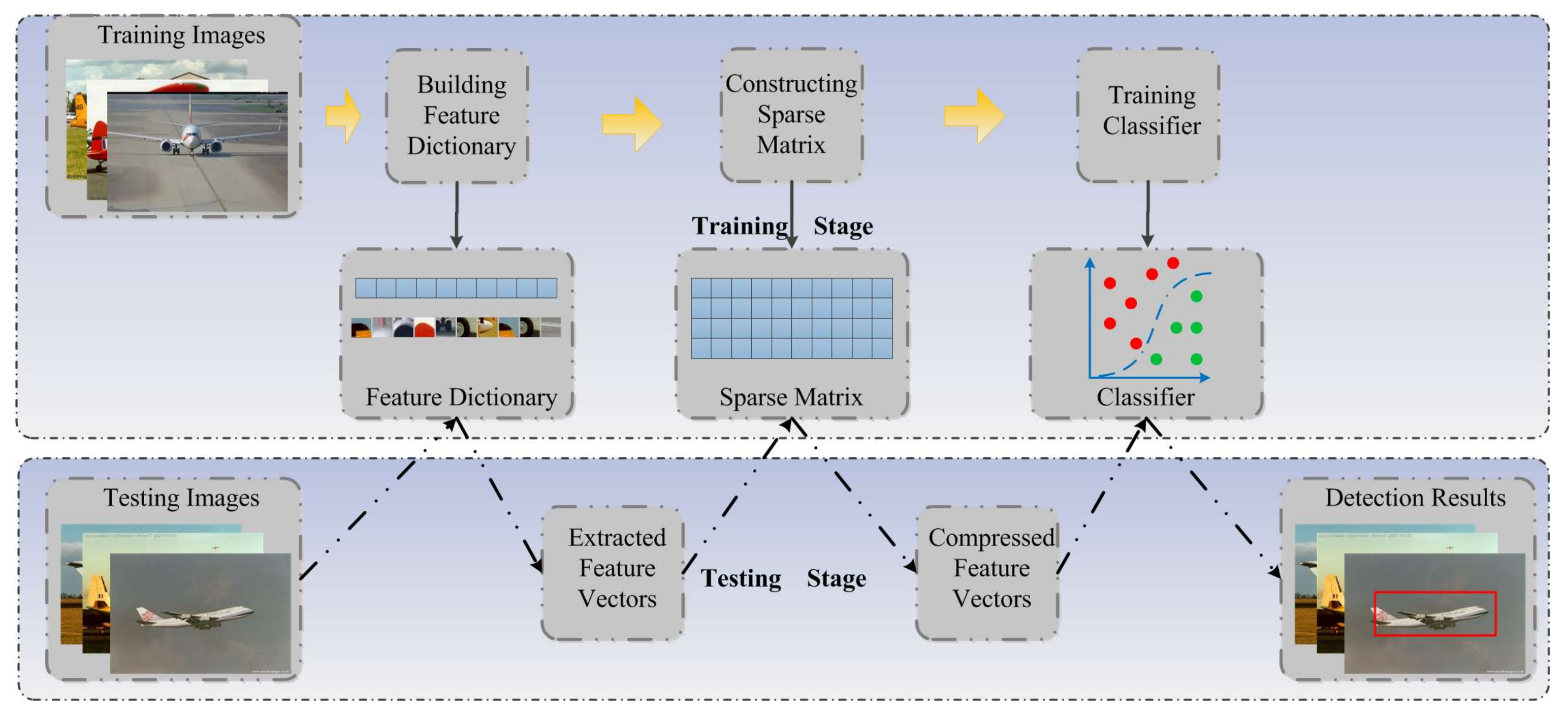
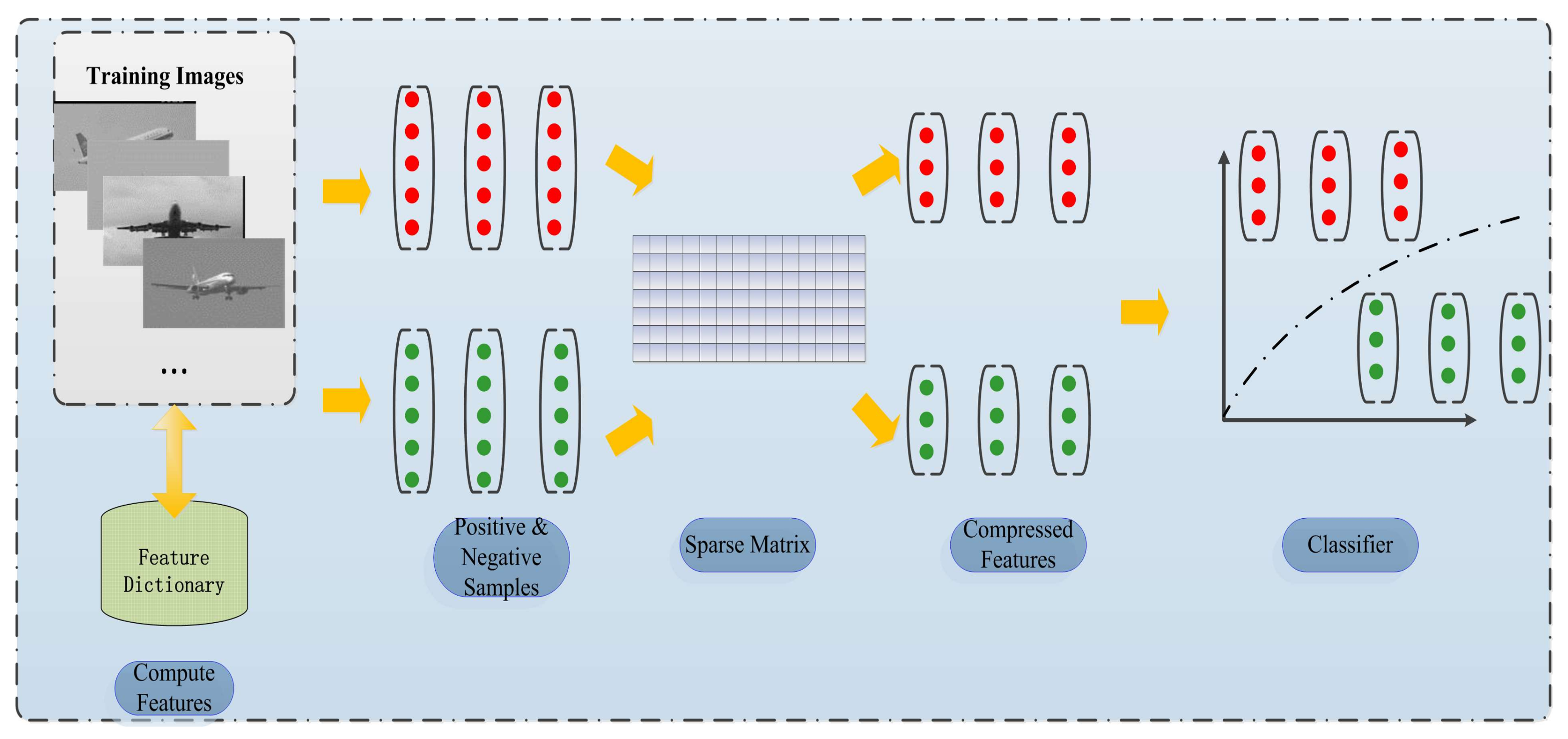
Figure 1. Framework of the proposed model.
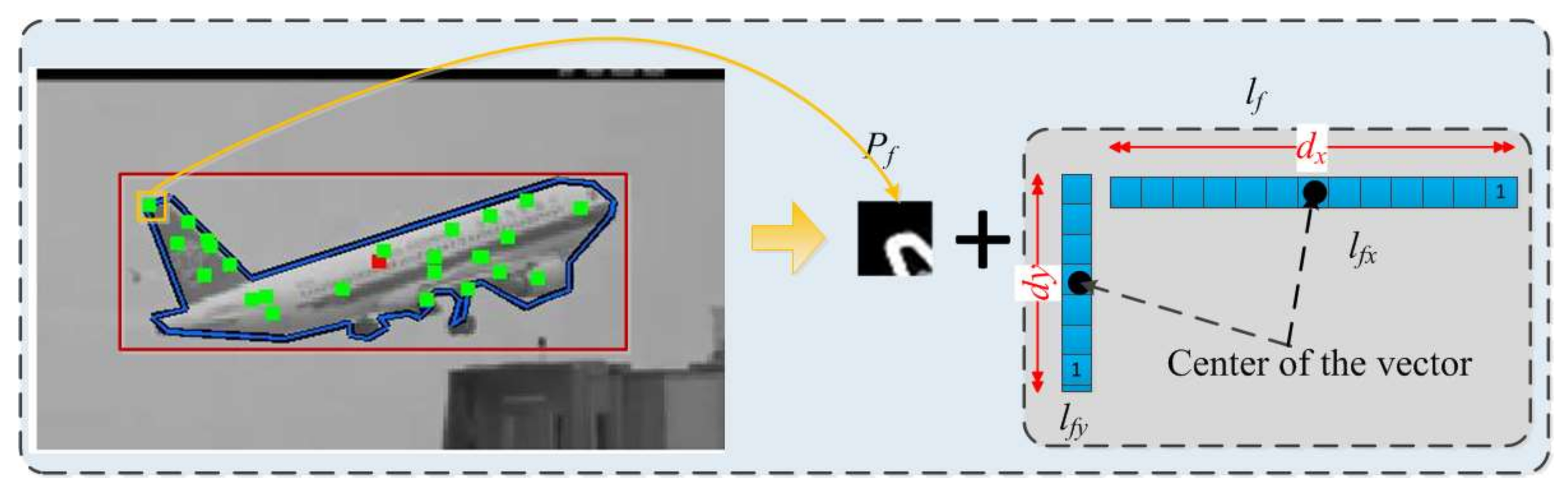
Information 09 00074 g001
Figure 2. The designed feature is combined an informative patch and two sparse vectors.
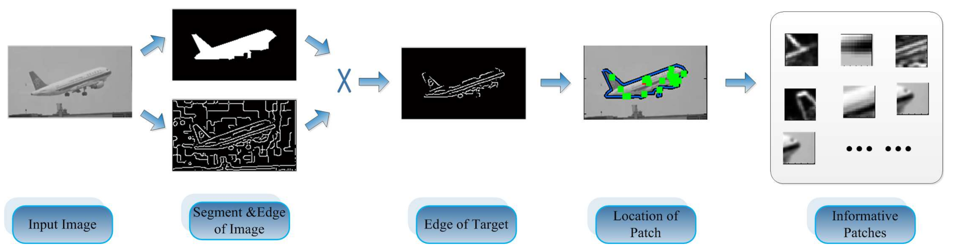
Information 09 00074 g002
Figure 3. The informative patches were extracted from the location which includes rich edge information.
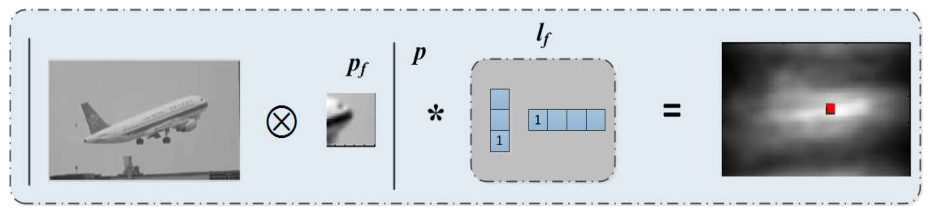
Information 09 00074 g003
Figure 4. A local informative patch is employed to construct feature vectors, from the picture in right column, object area has higher response than backgrounds.
Information 09 00074 g004
Figure 5. All of the feature vectors were compressed by a sparse matrix, and the compressed feature vectors were adopted to build the classifier.
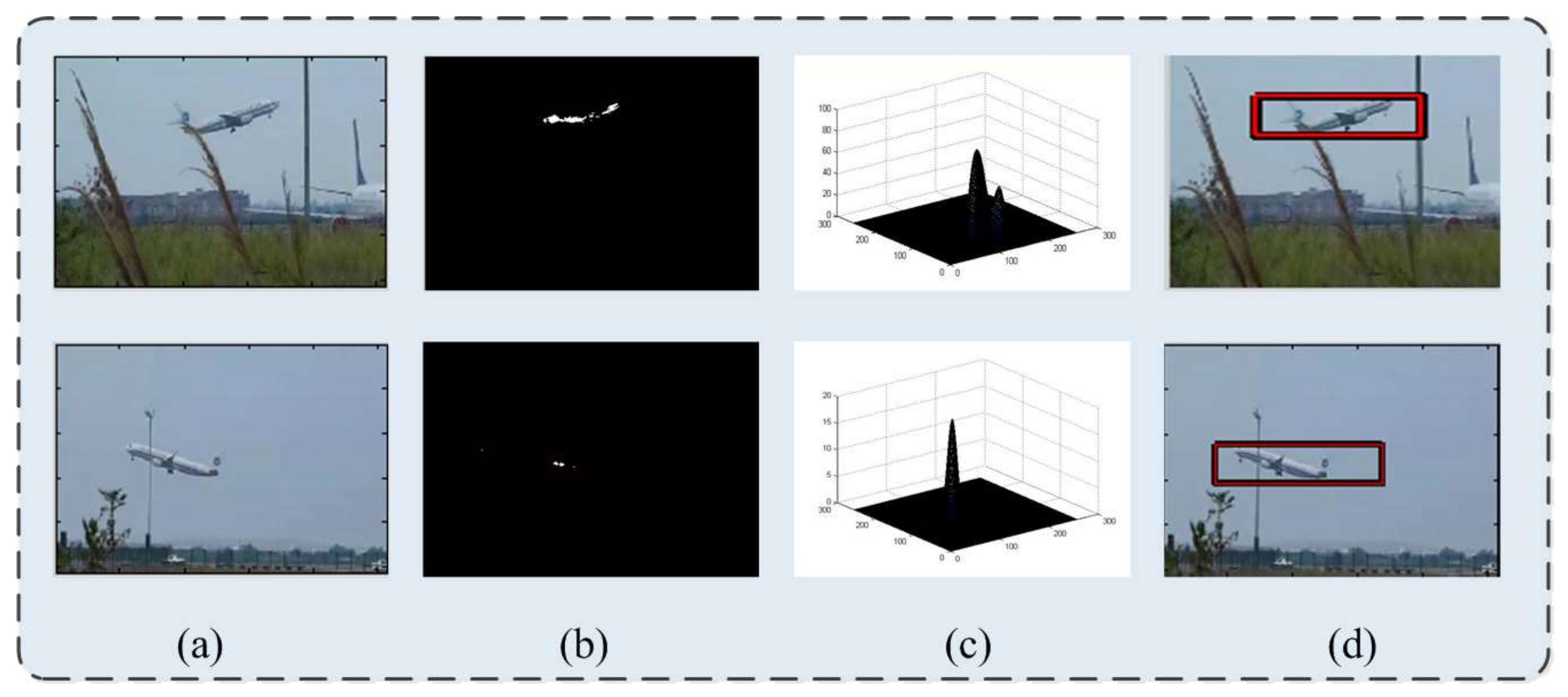
Information 09 00074 g005
Figure 6. (a) Testing image; (b) the score map calculated by classifier; (c) illustration of the distribution of the regional maxima; and (d) detection results.
Information 09 00074 g006
Figure 7. Examples from our moving aircraft database, the aircrafts appear in different scenes.
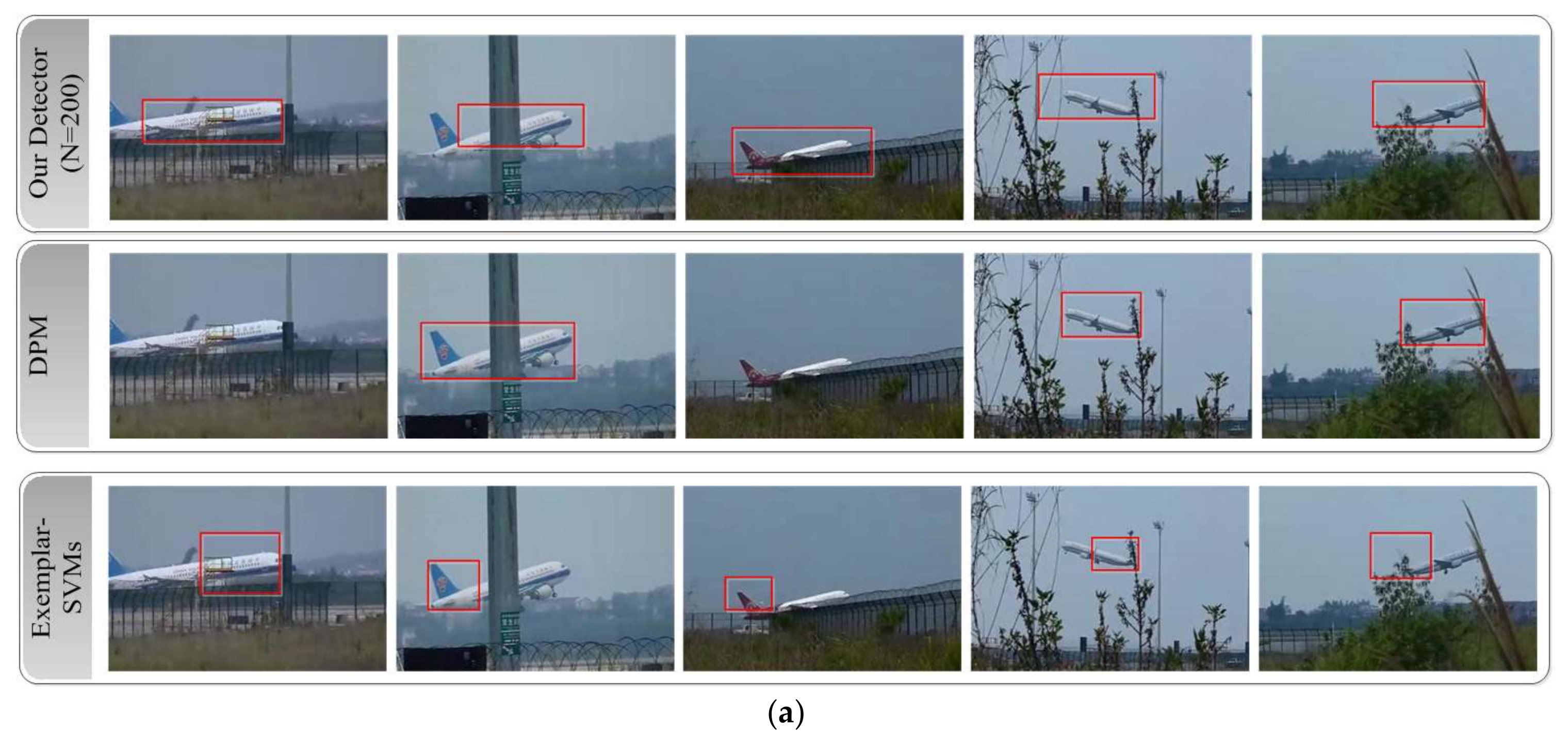
Information 09 00074 g007
Figure 8. (a) Illustration of the detection accuracy between our trained detectors (detector 1–4) and other models (DPM and exemplar-SVMs); and (b) the precision-recall curve.
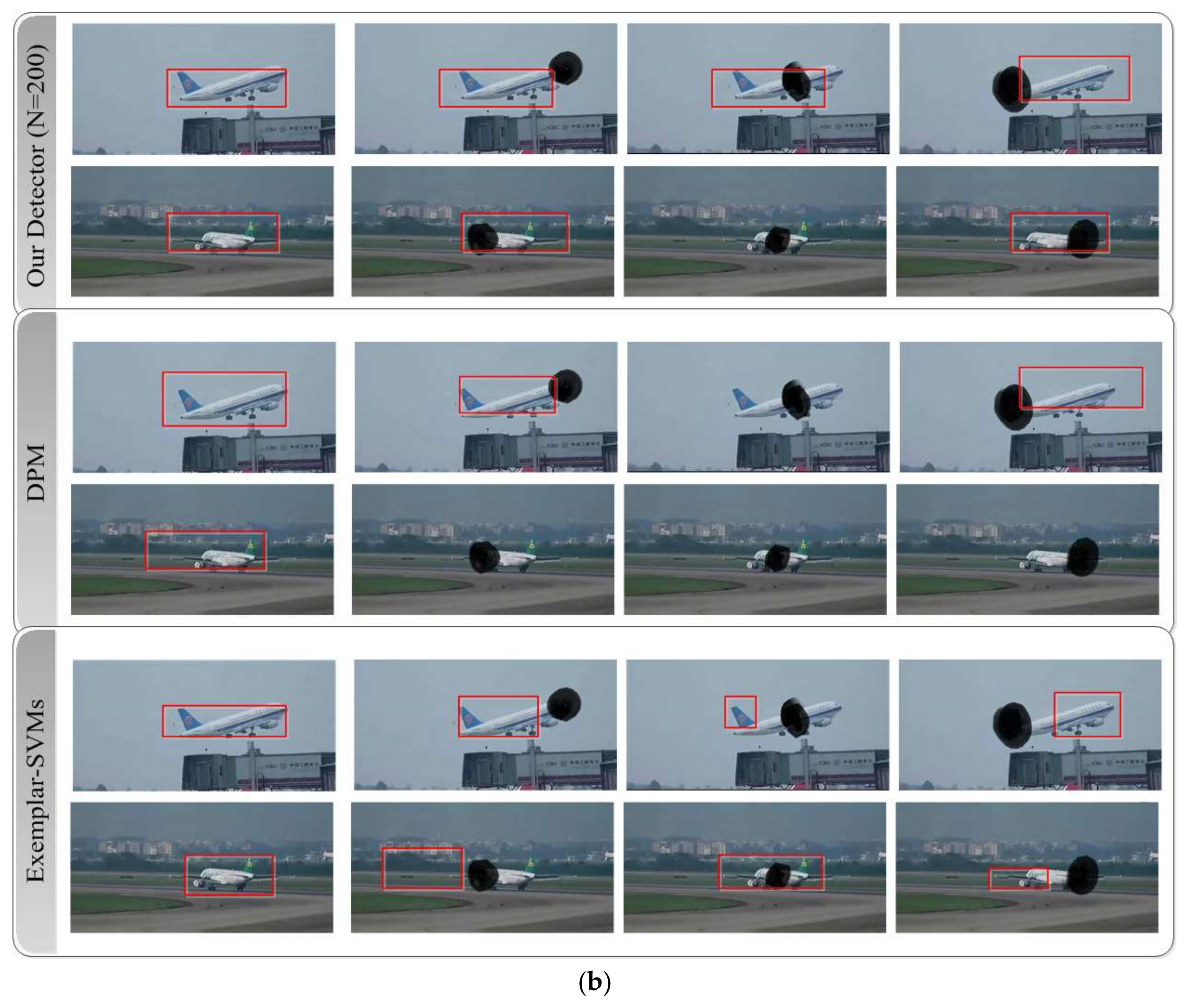
Information 09 00074 g008
Figure 9. (a) Detection results of partially-occluded aircrafts in original images; and (b) detection results of the aircrafts with manual occlusion in different parts (nose, body, and tail).
Information 09 00074 g009aInformation 09 00074 g009b
Figure 10. 
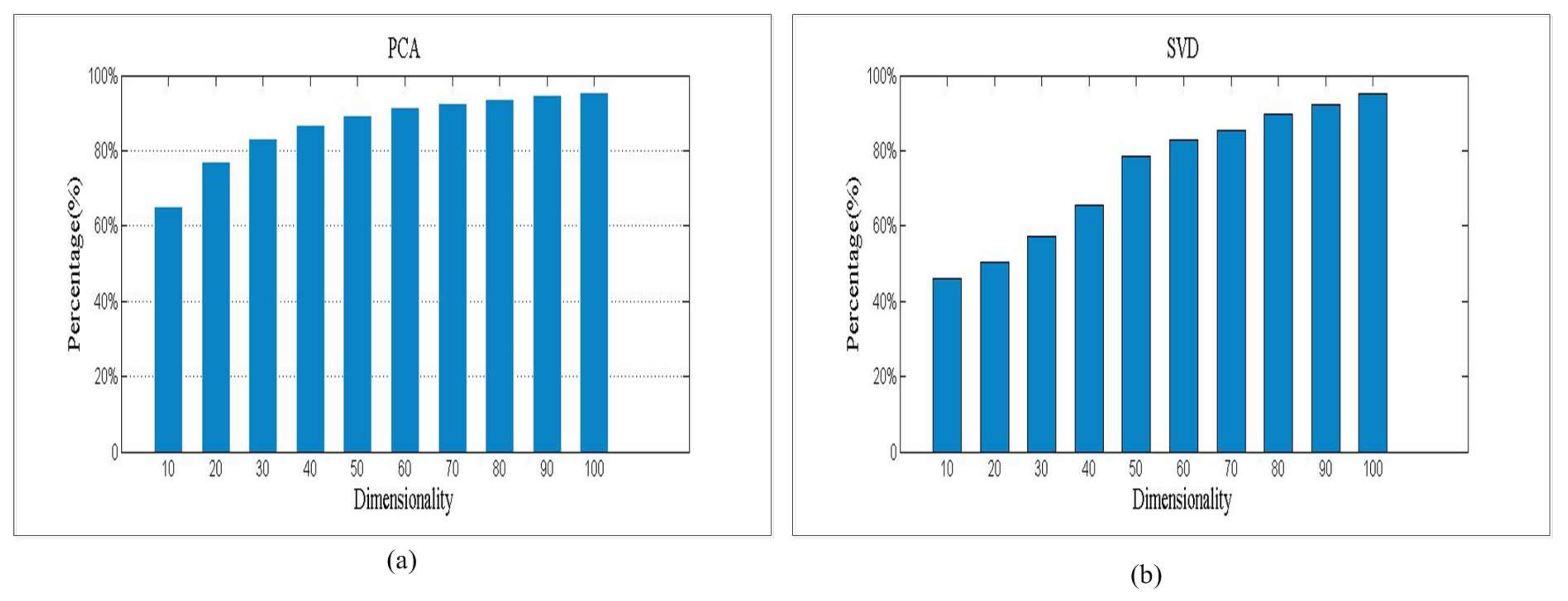
Information preservation percentages of (a) PCA, and (b) SVD.
Information 09 00074 g010
Figure 11. 
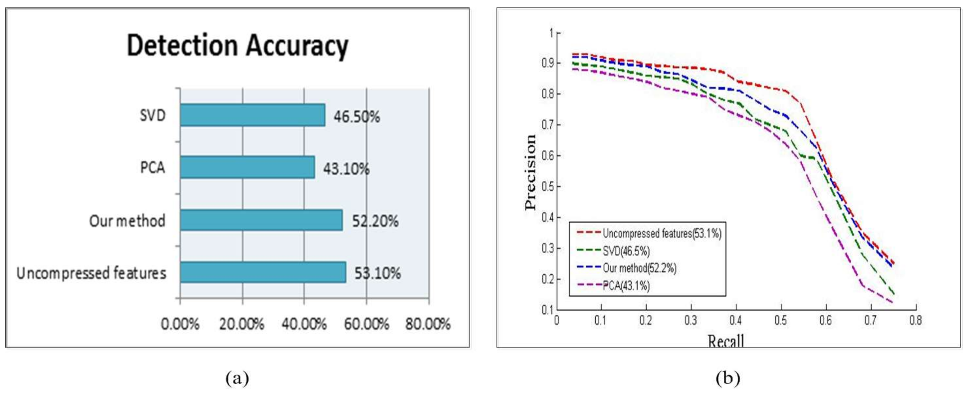
(a) Illustration of the detection accuracy of four kinds of features; and (b) the precision-recall curve.
Information 09 00074 g011
Figure 12. 
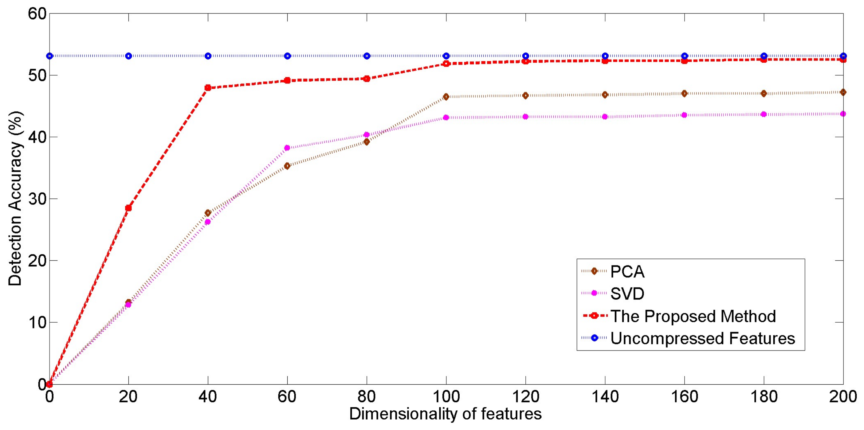
Illustration of the relationship between compressed dimensionality and detection accuracy.
Information 09 00074 g012
Figure 13. 
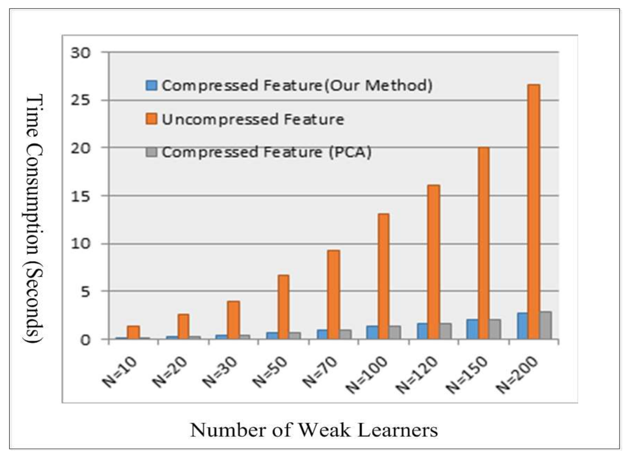
Time consumption of three kinds of features.
Information 09 00074 g013
Table 1. The process of building the informative feature dictionary.
Step 1: Segmenting the object with the background and calculating the centroid (cx, cy) of the object.
Step 2: Obtaining the image’s edge information by two 1-Dimensional masks [–1, 0, 1] and [–1, 0, 1]Transpose.
Step 3: Using the results of step 1 and step 2 to obtain the edge information of the object.
Step 4: Extracting the candidate patch (pf) at each location (lf) where holds an edge value calculated in step 3, and each extracted patch has a fixed size of 15 × 15 pixels.
Step 5: Adopting Non-Maximum Suppression (NMS) [31] to reduce the number of candidate patches.
Step 6: Performing k-means for the rest candidate patches.
Step 7: Selecting the clusters as the element of the informative patch dictionary.
Table 2. The process of collecting training samples.
Step 1: Scaling the another subset of training images in order to make the objects fit into the bounding box (of size 40 × 120 pixels);
Step 2: Cropping images in uniform size (e.g., 120 × 200 pixels);
Step 3: Performing normalized cross correlation between each patches and training images;
Step 4: Performing element-wise exponentiation of the result from step 3 with exponent p = 3;
Step 5: Convolving the result of step 4 with the patch’s location;
Step 6: Features at object’s centroid and background were represented as positive and negative samples, respectively.
Table 3. Comparison of three methods in partially-occluded object detection (%).
1 D1 (N = 50)D2 (N = 100)D3 (N = 150)D4 (N = 200)DPM [4]Exemplar-SVMs [5]
26.828.331.232.727.220.3
1 Note: D1, D2, D3, and D4 represent the four trained detectors with a specific number of weak learners.
Table 4. Experiments on Caltech 101 database (aircraft sub-category) (%).
D1 (N = 50)D2 (N = 100)D3 (N = 150)D4 (N = 200)DPMExemplar-SVMs
Original images35.839.842.743.932.845.8
Occluded images29.733.135.936.519.632.3
Table 5. Per image detection time of each detector (seconds).
D1 (N = 50)D2 (N = 100)D3 (N = 150)D4 (N = 200)DPMExemplar-SVMs
Detection time2.013.665.696.5727.5319.87
Table 6. Feature compression with three methods (milliseconds).
Time ConsumptionOur MethodPCASVD
100 D18.7656.3535.2
200 D20.2667.1551.8
400 D26.9695.6567.5
800 D45.6702.3579.7

