LICIC: Less Important Components for Imbalanced Multiclass Classification

Abstract

Multiclass classification in cancer diagnostics, using DNA or Gene Expression Signatures, but also classification of bacteria species fingerprints in MALDI-TOF mass spectrometry data, is challenging because of imbalanced data and the high number of dimensions with respect to the number of instances. In this study, a new oversampling technique called LICIC will be presented as a valuable instrument in countering both class imbalance, and the famous “curse of dimensionality” problem. The method enables preservation of non-linearities within the dataset, while creating new instances without adding noise. The method will be compared with other oversampling methods, such as Random Oversampling, SMOTE, Borderline-SMOTE, and ADASYN. F1 scores show the validity of this new technique when used with imbalanced, multiclass, and high-dimensional datasets.

1. Introduction

The between-class imbalance is a well-known problem that afflicts numerous datasets. The classification task become even more difficult if there are very few instances in the dataset, a few hundred for example, and when each instance is composed of thousands of dimensions. This other problem is well known in literature, and is called Bellman’s “curse of dimensionality”, which he describes as “a malediction that has plagued the scientist from earliest days” [1]. One simple solution, in addition to dimensionality reduction, is to add new data in the training set, in order to increase dataset size and balance the number of instances between classes.

Previously published works in [2,3,4,5], focused on the strong class imbalance and on the importance of the minority class. Real-world datasets, such as unreliable telecommunication customer’s dataset or datasets used to detect fraudulent telephone calls, directed attention to the correct classification of the minority class, and are often binary classification problems. In this study, all classes are treated with the same importance, and both studied datasets are designed for a multiclass classification task, in which all classes share the same “importance”. Consequently, the algorithm should not put any weight or importance on the number of instances in each class, but should be able to create synthetic instances that are representative of the underlying pattern for that class.

In this study, a new algorithm for imbalanced datasets is presented. This algorithm, called LICIC (Less Important Components for Imbalanced multiclass Classification), is designed to deal with datasets that have fewer instances than the number of dimensions, and where there is a strong skewness between the number of instances of different classes. It operates in “feature-space” rather than “data space”, preserving non-linearities present in datasets. It makes use of kernel PCA [6] on the whole dataset and works in Φ(x) transformed space, effecting permutations of less important components, to create new synthetic instances for each minority class. The permutation is performed between instances belonging to the same class.

The intuition is that, since eigenvalues in Φ(x) are ranked from most important to the least, applying a permutation on a ratio of components and on similar instances belonging to the same class, it is finally possible to create new synthetic instances. Those new instances look similar to the previous, but their least important components (in Φ(x) space) are the combination of other similar instances.

This is relevant because no new information nor randomness is added, unlike the majority of other algorithms used for managing class imbalance problems. As will be shown later, randomness and the addition of new, unknown, information could constitute the creation of synthetic noise and consequently, an increase in overfitting (learning the noise), and a decrease in the generalization power of the classification models.

This paper is organized as follows: Section 2 illustrates relevant works on class imbalance problems. Section 3 describes the datasets used in this study and their importance for the research community. Section 4 introduces principal component analysis and kernel principal component analysis with pre-image computation. Section 5 introduces the LICIC algorithm. Section 6 describes the experiments and results. Section 7 contains conclusions and reflections on future work.

2. Literature Review

The first attempt to increase the number of instances within the minority classes was Random Oversampling, which is a simple duplication (randomly selected with replacement) of instances. This solves the problem of class imbalance, but increases the chance of overfitting and, thus, decreases the capability of generalization [3].

In SMOTE [4], the authors propose the creation of new synthetic instances by using synthetic samples, taking the difference between the feature vector considered and its nearest neighbor. This difference is later multiplied with a random number [0, 1], and added to the feature vector in consideration.

In [3], the authors develop the idea of SMOTE to use SVM classifiers to deal with class imbalance problems; artificial minority class instances are generated around the borderline between two data classes. Those borderline data points are identified by support vectors. This is because borderline instances are more likely to be misclassified and expand the minority classes to areas where the density of majority classes is not high.

In [7], the authors define the concept of “safe region” and “unsafe region”. The newly generated instance is positioned closer to the largest “safe region”, therefore, if the safe level of an instance is close to 0, the instance is nearly noise. If it is close to a positive integer, the instance is considered safe. In [5], the authors describe ADASYN as a technique for adaptively generating minority data samples according to data distribution, where more synthetic data is generated for minority class samples that are harder to learn, compared to those minority samples that are easier to learn.

In [8], the authors describe examples defined “hard”, coming from the majority and minority classes during the process of boosting, which are then used to generate new synthetic data. In [9], the authors partition the majority class into clusters and, then, for each cluster, increase the size of the training set for that cluster with SMOTE. They use SVM, Decision Trees, and ANN for checking classification accuracy. In [10], the authors use SMOTE to alleviate the class imbalance problem for multiclass classification for Gene Function Prediction.

As it is possible to note, almost all related works focus on finding examples that are, in some way, hard to classify and replicate. LICIC does not provide any assumptions regarding the hardness of each instance to be classified per class, sustaining the assumption that data is I.I.D. This may seem counterintuitive, and a step back in research but, as will be shown later, the process of KPCA and non-linear noise removal built in the algorithm can be exploited to limit hard examples (which generate noise alone), and better define the particular pattern of that class. In this way, they generalize on the creation of new synthetic instances.

In previous studies [11,12,13]], the authors of this paper have worked on Expert Systems, ensemble techniques, and pattern recognition for several problems. They have dealt with issues ranging from signature verification to heartbeat classification for detecting arrhythmias, where the majority of datasets used suffered from a strong class imbalance problem.

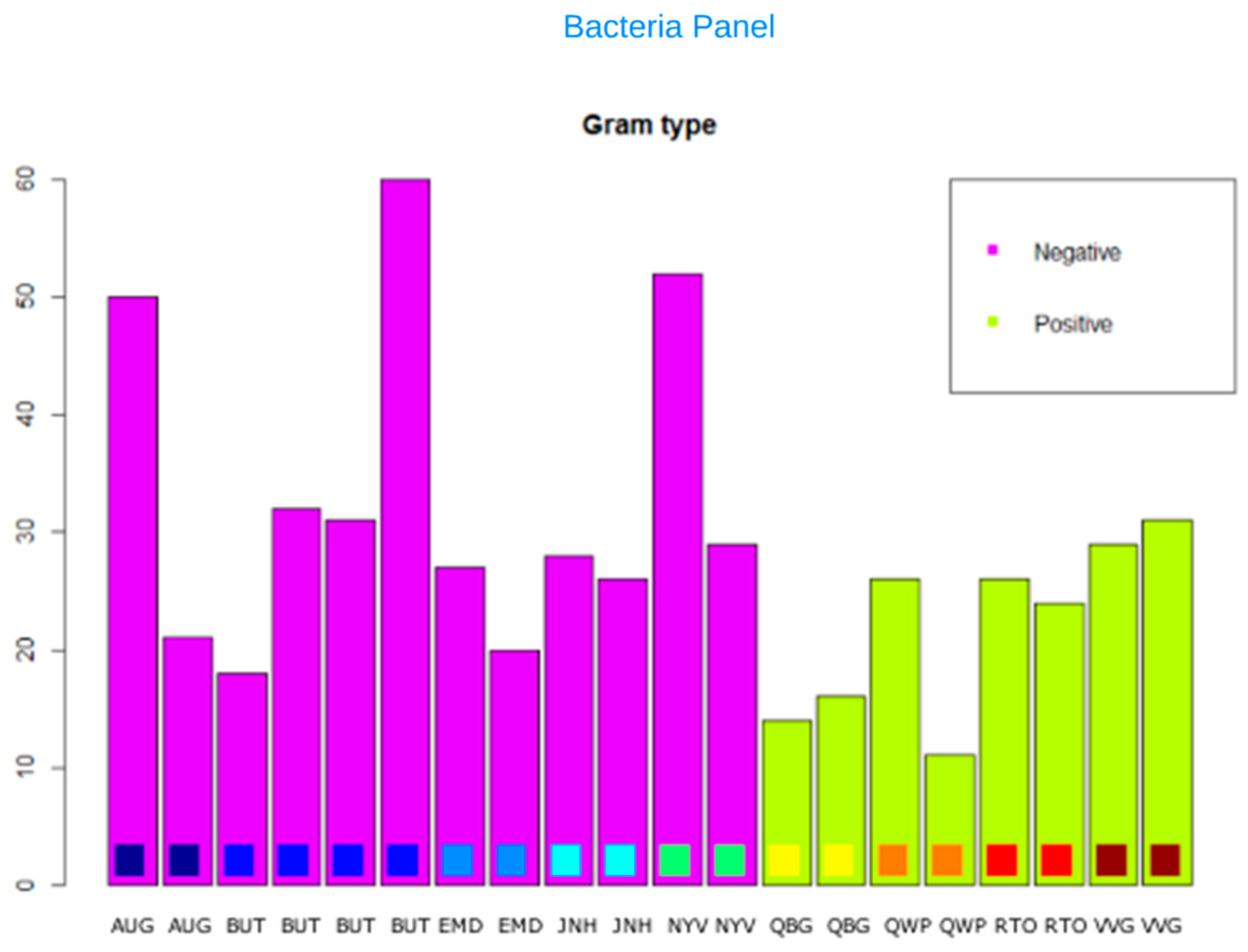
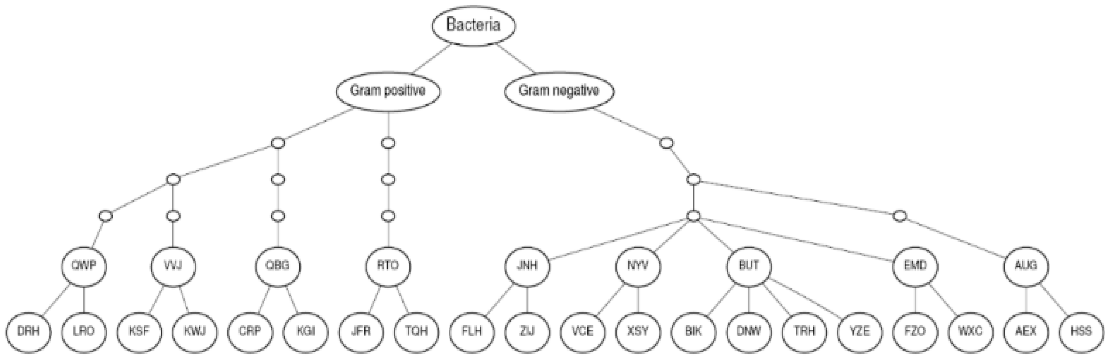
3. Dataset Description

Medical datasets, like the MicroMass MALDI-TOF dataset [14,15] and the Gene Expression Signatures for Multiclass Cancer diagnosis dataset (GCM), are composed of 931 instances with 1300 dimensions for MicroMass and 218 instances with 16,063 dimensions for GCM, respectively. Neither dataset have missing values, both have some undescribed amount of noise, caused by the transcription machine but, more importantly, each instance in both datasets represents a human being for GCM and a particular bacterium for MicroMass. The MicroMass dataset is composed of a reference panel of 20 Gram-positive and -negative bacterial species covering 9 genera, among which several species are known to be hard to discriminate with mass spectrometry (MALDI-TOF). Each species was represented by 11 to 60 mass spectra obtained from 7 to 20 bacterial strains, constituting a dataset of 571 spectra obtained from 213 strains. The spectra were obtained according to the standard culture-based workflow used in clinical routine, in which the microorganism was first grown on an agar plate for 24 to 48 h, before a colony portion was harvested, spotted on a MALDI slide, and a mass spectrum was acquired [16].

The GCM dataset needs further explanation—as of now, cancer classification relies on the subjective interpretation of both clinical and histopathological information, and its correct classification is, therefore, the responsibility of the oncologist. Unfortunately, clinical information can be incomplete or misleading. In addition, there is a wide spectrum in cancer morphology and many tumors are atypical or lack morphologic features useful for differential diagnosis.

These difficulties can result in diagnostic confusion, prompting calls for mandatory second opinions in all surgical pathology cases [17]. The challenge of using this dataset is to extract complex patterns able to correctly classify cancer, starting from DNA gene expression profiles, and thus enable a precise, objective, and systematic human cancer classification avoiding dependency on the oncologist’s experience that may vary and is non-deterministic. The GCM dataset contains DNA microarray-based tumor gene expression profiles, in which each instance is the gene expression of a human tumor cell. It is composed of 16,063 numerical features with only 218 instances and 14 tumor classes: breast adenocarcinoma, prostate adenocarcinoma, lung adenocarcinoma, colorectal adenocarcinoma, lymphoma, bladder transitional cell carcinoma, melanoma, uterine adenocarcinoma, leukemia, renal cell carcinoma, pancreatic adenocarcinoma, ovarian adenocarcinoma, pleural mesothelioma, and central nervous system.

In the literature, works [18,19,20,21,22,23,24] have shown that, despite the high number of dimensions in RNA sequencing, DNA and Gene Expression Profiles datasets, an accurate classification is feasible if class imbalance is treated appropriately.

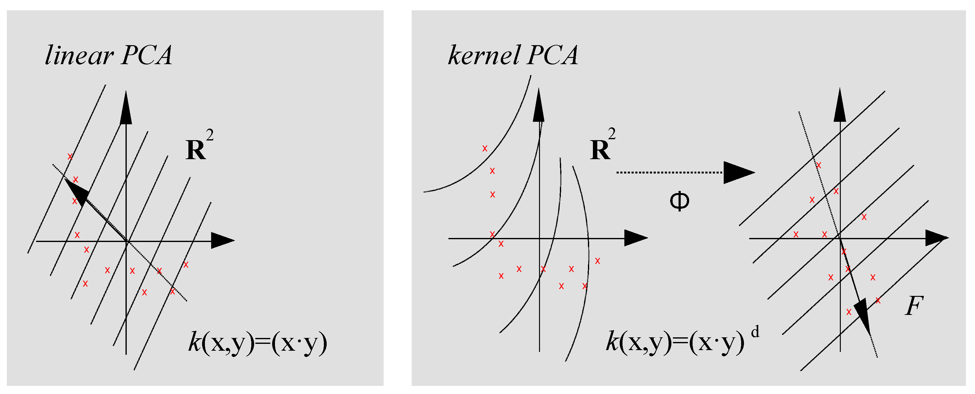
4. Kernel Principal Components Analysis with Pre-Image Computation

The importance of KPCA integrated within LICIC must be sought by looking at the intuition behind KPCA (and PCA for linear datasets), where the aim is to find axes with maximum variances along which the data is most spread. These axes are the principal components, and are represented as column rows of the classification matrix.

The basic concepts of orthonormal and orthogonal axes generalize the concept of a reference system on the Cartesian plane, and make it possible to define perpendicular axes and a reference system that is assigned to each point and its coordinates, on a vector space with arbitrary dimension.

Using orthonormal axes (the principal components), old features are synthetized into new features by projecting them onto those axes. These new features are orthonormal, and maximize the distance between them, which means that the ratio of less important components used in LICIC, as will be shown later, capture mostly minor diversity (borderline diversity) and a small amount of noise between instances of the same class. The basic idea in dealing with linearly inseparable data is to project it onto a higher dimensional space where it becomes linearly separable. Let us call this non-linear mapping function ϕ, so that the mapping of a sample x can be written as

x → ϕ(x),

which is the “kernel function”.

The term “kernel” describes a function that calculates the dot product of the images of the samples x under ϕ.

κ(x_i,x_j) = ϕ(x_i)ϕ(x_j)^T

In other words, the function ϕ maps the original d-dimensional features into a larger, k-dimensional feature space by creating non-linear combinations of the original features. Often, the mathematical definition of the RBF kernel is written and implemented as

κ(x_i,x_j) = exp(−γ∥x_i−x_j∥₂²)κ(x_i,x_j) = exp(−γ‖x_i−x_j‖₂²),

where $\mathsf{\gamma }=\frac{1}{2{\sigma }^2}$ is a free parameter that is to be optimized [25].

Scholkopf, Smola, and Muller, in [6], generalized this approach for data that was mapped onto the higher dimensional space via a kernel function as shown in Figure 1:

$$\mathrm{Cov}=\frac{1}{\mathrm{n}}{\displaystyle \sum }_{\mathrm{i}=1}^{\mathrm{n}}\varphi \left({\mathrm{x}}_{\mathrm{i}}\right)\varphi {\left({\mathrm{x}}_{\mathrm{i}}\right)}^{\mathrm{T}}$$

However, in practice, the covariance matrix in the higher dimensional space is not calculated explicitly (kernel trick). Therefore, the implementation of RBF kernel PCA does not yield the principal component axes (in contrast to the standard PCA), but the obtained eigenvectors can be understood as projections of the data onto the principal components. [25]

In [26], the pre-image problem is defined as follows: given a point Ψ in H_k, the goal is to find the corresponding pattern x ∈ X, such that Ψ = φ(x). However, since the kernel space is much larger than feature space, it is often not possible. The pre-image is calculated first obtaining the principal components in kernel space and then learning the map from:

φk(x) to (φl(y)Tv1, …, φl(y)Tvr).

For each principal component v. At the end, there is a testing phase where the learned map is used to approximate the pre-image of the estimated point φ(y’) in H₁.

This technique has been widely tested, and is very useful for signal compression and de-noising.

5. LICIC Algorithm

In order to avoid bleeding information into the test set, the following algorithm is applied only to the training set. The algorithm is shown in Box 1. In order to preserve the non-linearities, KPCA can be executed with one of the desired kernels (depending on the nature of the problem), but it is also possible to perform a non-linear low rank approximation to decrease the number of components in training_set, thus removing the noise, if present. Each component on the KPCA-transformed training set, called training_set, is ordered from the most to the least important. The algorithm then choses the last components (the amount is defined by the ratio value) and performs the permutation of n (where n = components_to_use/k) components with k similar instances, similar to the one randomly selected per class. Finally, this new instance, having last components made as the permutation of components of similar instances, is added to the training_set’. In this way, differently from SMOTE (and its variations) and ADASYN, no new information is added (it is a permutation), and noise can be removed.

Box 1. LICIC algorithm.

The process ends when the number of instances in the new training_set’ per class is equal to the number of instances within the most numerous class multiplied by a parameter called ratio_instance, which indicates how much has been decided to increase the training set size. This ratio_instance is used to uniformly increase the number of instances in all classes. If equal to 1.0, then the number of instances for each class will be equal to the number of instances in the most numerous class. Otherwise, if ratio_instances > 1.0, new synthetic instances will be produced for the most numerous class too.

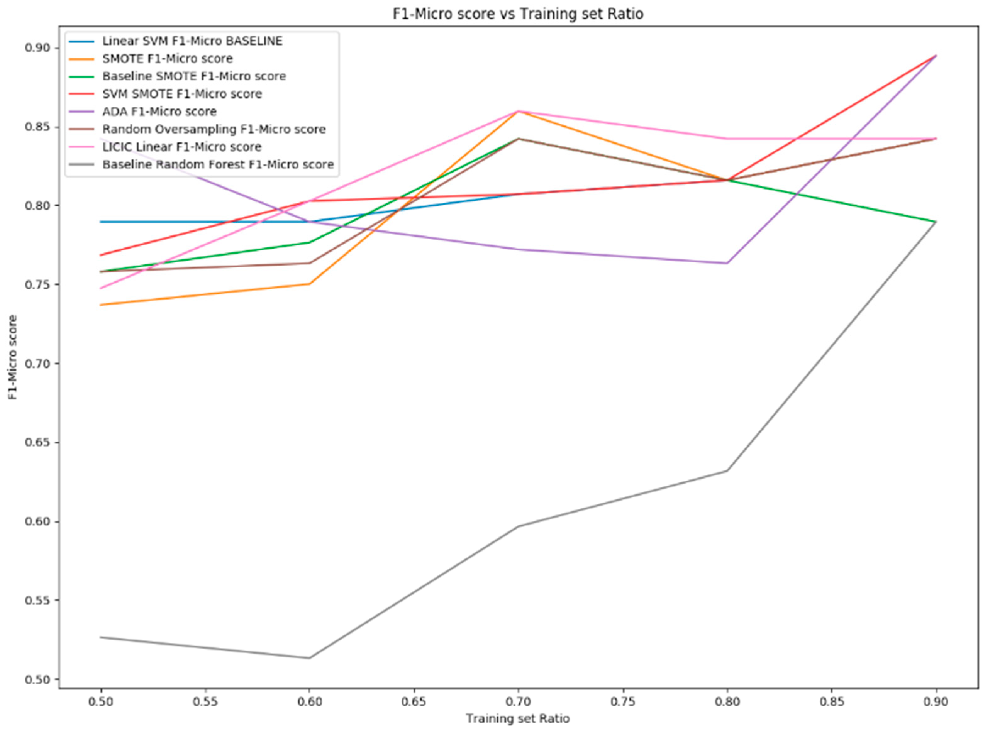
6. Experiments and Results

For both datasets, a few common strategies have been employed. Both datasets are randomly shuffled and separated into two parts: the training set, which contains 70% of the dataset, and a test set, which contains the remaining 30%. The size of training set will be varied and reported during analysis.

It is known that Support Vector Machine is the preferred algorithm to deal with an imbalanced dataset, and is also the reference algorithm used in [17] for classifying tumors in GCM dataset, therefore, the SVM accuracy will be used as a baseline for comparison purposes. For MicroMass dataset, the Random Forest classifier will be used as the main classification model, configured with 100 estimators and depth of 10. This pre-pruning parameter is used to determine the maximum depth of the tree, and is used to avoid overfitting by limiting its depth during the construction of the tree. Entropy is used as an impurity measure (splitting criteria) as it attempts to maximize the mutual information in the tree. For GCM dataset, Linear SVM, as reported in [17], will be used as the main classification algorithm.

The model is trained on the training part only, no data points from the test part were used while training or computing feature normalization (this statement holds also for cross-validation). 10-Fold Cross-Validation performance was calculated on training set. For both datasets, the F1-Micro score is computed. F1-Micro score is used in medicine, where a false negative (the person has the disease but the system says not) is worth more than a false positive (the system says the person has the disease but this is not true). For the multiclass problem defined in GCM and MicroMass datasets, a F1-Micro scoring metric has been employed, defined as the harmonic mean between precision and recall of all classes, weighting each instance equally. F1-Micro is thus best suited for imbalanced datasets like this, and is effective in comparing the final F1-Micro score with the F1-Micro score provided by SVM which represents the baseline. The random prediction accuracy for GCM is 1/14 = 0.071, 7.1%, where 14 is the number of classes. For MicroMass dataset it is 1/20 = 0.05, 5%, where 20 is the number of classes.

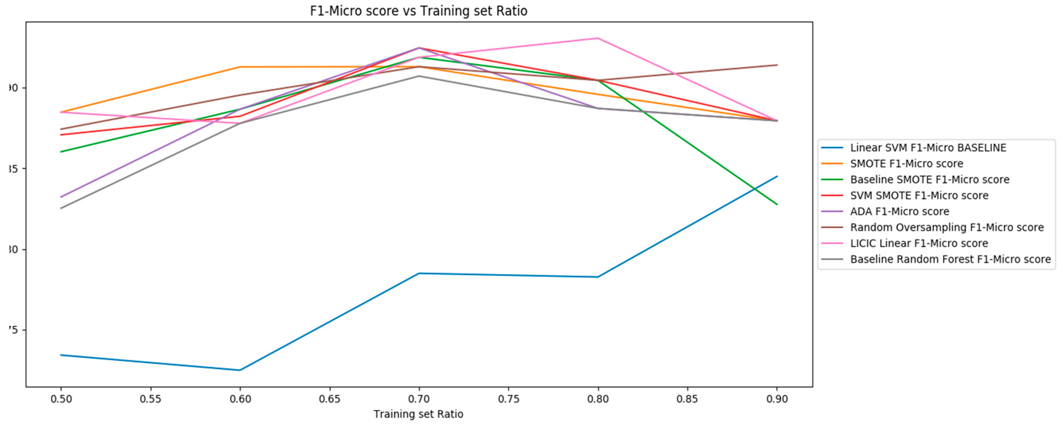
6.1. MicroMass Dataset Results

Figure 2 shows F1-Micro score on both the Test Set and in Cross-Validation for Linear SVM, which is used as the overall baseline comparison, with Random Forest Classifier without LICIC, with Random Forest Classifier with LICIC the following kernels: Linear, RBF kernel with gamma = 0.1, and polynomial kernel with degree = 3, reported with their respective Cross-Validation F1-Micro scores.

All Random Forest Classifiers were setup with 100 estimators and 10 max depths as pre-pruning parameter.

Looking at scores on Test Set, LICIC with linear KPCA achieved the highest F1-Micro score with 0.9370 with a ratio equal to 0.4 (the green line), even if the cross-validation score of LICIC with linear KPCA is 0.9722. This is a difference of 0.0352, smaller than others, showing that for this particular problem LICIC with linear KPCA is well suited. The chart also shows that the Linear SVM F1-Micro score on test set (blue line) is lower compared to the Random Forest score on same data (orange line). Thus Random Forest classifier is preferred to SVM on this dataset. LICIC with Polynomial KPCA achieved a bad accuracy (fuchsia color) together with LICIC with RBF kernel (violet line), even though their respective cross-validation accuracy was high, demonstrating a profound overfitting of LICIC when data that can be treated linearly, is treated non-linearly.

The following test will be conducted with LICIC having linear KPCA and a component ratio of 0.4.

Figure 3 shows the learning curve for the F1-Micro score on test set for different class imbalance handling algorithms while varying the ratio of the training set size. Those algorithms are SMOTE (orange line), Baseline SMOTE (green line), SVM SMOTE (red line), ADASYN (violet line), Random Oversampling (brown line), LICIC (fuchsia line). All Random Forest Classifiers were setup with 100 estimators and 10 max depths as pre-pruning parameter.

Linear SVM without any imbalance learning algorithm (blue line) is used as a baseline together with Random Forest Classifier (green line) trained without any class imbalance algorithm. SMOTE, Borderline SMOTE, SVM SMOTE, ADASYN and LICIC tests were conducted with K = 5 as number of nearest neighbors.

Figure 3 shows that when the ratio of the training set is 80% of the whole dataset, the F1-Micro score on test set is 0.9302 which is higher with respect to all other algorithms analyzed. When training set ratio is equal or less than 60%, SMOTE and SVM SMOTE seem to do a better job on generalizing. It is also interesting to note that all algorithms for class imbalance outperformed the baseline Random Forest Classifier and also the SVM Linear classifier.

Figure 4 and Figure 5 show that QWP.LRO and QWP.DRH are very close genera. Figure 6 shows that almost all classes are correctly classified but QWP.LRO is always confused with QWP.DRH.

6.2. GCM Dataset Results

Figure 7 shows the F1-Micro score on both Test Set and in Cross-Validation for Linear SVM, which is used as the overall baseline comparison, with Random Forest Classifier without LICIC, with Linear SVM with LICIC Linear, Linear SVM with LICIC RBF kernel with gamma = 0.1 and Linear SVM with LICIC Polynomial kernel with degree = 3 with their respective Cross-Validation scores. Because the accuracies of Random Forest Classifier on this dataset are lower compared to linear SVM (respectively yellow line vs. blue line), Linear SVM has therefore been used, together with LICIC algorithm with different types of kernels.

The Linear SVM baseline F1-Micro score is similar to the score achieved in [17] which is 0.8002. In [4] the authors reported 0.79, however the differences might be due to randomization and improvement achieved by new SVM libraries. As it is possible to note, even on this dataset LICIC with linear KPCA is preferred over LICIC with RBF kernel with gamma = 0.1 or Polynomial Kernel with degree = 3. It is also important to note that the difference between LICIC with Linear KPCA F1-Micro score on test set and its cross-validation score, is smaller compared to the difference for LICIC with RBF KPCA and its corresponding Cross-Validation score, and the same for LICIC with Polynomial KPCA. The highest F1-Micro score on test set was achieved for ratios 0.5 and 0.6 which was 0.8421, therefore 0.6 was the chosen ratio for comparing LICIC with other class imbalance algorithms. In particular, cross-validation score and test set score difference is almost zero when LICIC is set up with 0.6 as ratio for less important components. This is important because it shows that the model functions best without overfitting.

Figure 8 shows the learning curve for the F1-Micro score on test set for different class imbalance handling algorithms when varying the ratio of the training set size: SMOTE (orange line), Baseline SMOTE (green line), SVM SMOTE (red line), ADASYN (violet line), Random Oversampling (brown line), LICIC (fuchsia line). All algorithms utilized Linear SVM classifier. For a better readability, the same results are also presented in

Table 1. Learning rate of several class imbalance methods with respect to training set ratio.

	Training-Set Ratio	50% of Dataset as Training Set	60% of Dataset as Training Set	70% of Dataset as Training Set	80% of Dataset as Training Set	90% of Dataset as Training Set
Algorithm
Linear SVM		0.7736	0.7736	0.8002	0.80914	0.82361
SMOTE		0.7368	0.7452	0.8603	0.80914	0.8746
Baseline SMOTE		0.7574	0.7682	0.8325	0.80914	0.7732
SVM SMOTE		0.7632	0.8002	0.8002	0.80914	0.8746
ADASYN		0.8435	0.7736	0.7631	0.7547	0.8746
Random Oversampling		0.7574	0.7532	0.8325	0.80914	0.8378
LICIC		0.7463	0.8002	0.8603	0.8423	0.8378
Baseline Random Forest		0.5321	0.5267	0.6002	0.6367	0.7732

.

The Linear SVM without any imbalance algorithm (blue line) is used as a baseline together with Random Forest Classifier (green line) trained without a class imbalance algorithm. SMOTE, Borderline SMOTE, SVM SMOTE, ADASYN and LICIC tests were conducted with K = 5 as number of nearest neighbors. As it is possible to note, on average LICIC outperforms all other techniques with training set size ranging from 60% to 80% of the whole dataset. LICIC also reaches the maximum peak in the interval at 80%, (the 90% interval is not considered because the test set size is too small to be determinant), with a F1-Micro score of 0.8603 increasing the F1-Micro score by circa 6 percentile points with respect to the Linear SVM on the original dataset with similar training set, test set split size [17]. This test also confirms that LICIC is a valid class imbalance algorithm only when there is an imbalanced, but a sufficient (It depends on Dataset) number of, instances in the training set.

Figure 9 shows the overall capability to recognize patterns among different cancer types. It is interesting to analyze that few cancer types, such as Colorectal and Pleural Mesothelioma, are confused 50% of the time by the classifier.

Pattern recognition techniques which reveal class imbalance techniques can be used to classify tumors starting from DNA sequences.

LICIC has improved the score on this dataset from 0.8002 to 0.8603 when the training set size is 70~80% of the whole dataset, setting new accuracy levels for the state of the art on this dataset. With a similar ratio, all other algorithms have also outperformed the SVM baseline. This result shows the importance of balancing a high dimensional multiclass dataset like this, creating synthetic instances which are not completely new (SMOTE) or a copy (Random Oversample) of other instances, but a modified version of original instances produced by permutation of less important components in Φ(x) space [26].

7. Conclusions

Despite the number of parameters needed to configure it properly, LICIC has shown to be a valuable tool for the scientist when analyzing imbalanced datasets and datasets with few instances. In particular, it has shown that LICIC with Linear KPCA is useful when the number of dimensions is very high. It is important to note the difference between cross-validation scores and the F1-Micro score calculated on test set on LICIC algorithm and all other algorithms used. This difference shows that overfitting is less pronounced when LICIC is used with respect to other imbalanced learn algorithms. Figure 7 shows that, for the ratio of components equal to 0.6, there is no overfitting, and the model operates best.

LICIC also shows its effectiveness when there is a sufficient amount of instances per class (e.g., 70% of dataset reserved for training set) to better define the particular pattern of that class and generalize on the creation of new synthetic instances.

Future work will test LICIC on highly non-linear datasets in order to show the effectiveness of KPCA with RBF kernel used in conjunction with LICIC for in-class pattern identification, and on the MNIST hand written digit dataset, in order to visually represent what new synthetic instances built by LICIC will look like and compare them to original instances.

References

1. Bellman, R.E. Adaptive Control Processes: A Guided Tour; Princeton University Press: Princeton, NJ, USA, 2015. [Google Scholar]
2. Han, H.; Wang, W.; Mao, B. Borderline-SMOTE: A new over-sampling method in imbalanced data sets learning. In Proceedings of the International Conference on Intelligent Computing, Hefei, China, 23–26 August 2005; Springer: Berlin/Heidelberg, Germany, 2005; pp. 878–887. [Google Scholar]
3. Nguyen, H.M.; Cooper, E.W.; Kamei, K. Borderline over-sampling for imbalanced data classification. In Proceedings of the Fifth International Workshop on Computational Intelligence & Applications, Milano, Italy, 7–10 September 2009; pp. 24–29. [Google Scholar]
4. Chawla, N.V.; Bowyer, K.W.; Hall, L.O.; Kegelmeyer, W.P. SMOTE: Synthetic Minority Over-sampling Technique. JAIR 2002, 16, 321–357. [Google Scholar] [CrossRef]
5. He, H.; Bai, Y.; Garcia, E.A.; Li, S. ADASYN: Adaptive synthetic sampling approach for imbalanced learning. In Proceedings of the 2008 IEEE International Joint Conference on Neural Networks (IEEE World Congress on Computational Intelligence), Hong Kong, China, 1–8 June 2008; pp. 1322–1328. [Google Scholar]
6. Schölkopf, B.; Smola, A.; Müller, K.R. Kernel principal component analysis. In Proceedings of the International Conference on Artificial Neural Networks, Lausanne, Switzerland, 8–10 October 1997; pp. 583–588. [Google Scholar]
7. Bunkhumpornpat, C.; Sinapiromsaran, K.; Lursinsap, C. Safe-level-smote: Safe-level-synthetic minority over-sampling technique for handling the class imbalanced problem. In Proceedings of the Pacific-Asia Conference on Knowledge Discovery and Data Mining, Bangkok, Thailand, 27–30 April 2009; pp. 475–482. [Google Scholar]
8. Guo, H.; Viktor, H.L. Learning from Imbalanced Data Sets with Boosting and Data Generation: The DataBoost-IM Approach. ACM Sigkdd Explor. Newslett. 2004, 6, 30–39. [Google Scholar] [CrossRef]
9. Guo, H.; Zhou, J.; Wu, C.-A. Imbalanced Learning Based on Data-Partition and SMOTE. Information 2018, 9, 238. [Google Scholar] [CrossRef]
10. Feng, S.; Fu, P.; Zheng, W. A Hierarchical Multi-Label Classification Algorithm for Gene Function Prediction. Algorithms 2017, 10, 138. [Google Scholar] [CrossRef]
11. Impedovo, D.; Pirlo, G. Updating knowledge in feedback-based multi-classifier systems. In Proceedings of the 2011 International Conference on Document Analysis and Recognition (ICDAR), Beijing, China, 18–21 September 2011; pp. 227–231. [Google Scholar]
12. Pirlo, G.; Trullo, C.A.; Impedovo, D. A feedback-based multi-classifier system. In Proceedings of the 10th International Conference on Document Analysis and Recognition, ICDAR’09, Barcelona, Spain, 26–29 July 2009; pp. 713–717. [Google Scholar]
13. Dentamaro, V.; Impedovo, D.; Pirlo, G.; Vessio, G. A new ConvNet architecture for heartbeat classification. In Proceedings of the ICPRAI, Montréal, QC, Canada, 14–17 May 2018. [Google Scholar]
14. Mahé, P.; Arsac, M.; Chatellier, S.; Monnin, V.; Perrot, N.; Mailler, S.; Girard, V.; Ramjeet, M.; Surre, J.; Lacroix, B.; et al. Automatic identification of mixed bacterial species fingerprints in a MALDI-TOF mass-spectrum. Bioinformatics 2014, 30, 1280–1286. [Google Scholar] [CrossRef] [PubMed] [Green Version]
15. Vervier, K.; Mahé, P.; Veyrieras, J.B.; Vert, J.P. Benchmark of structured machine learning methods for microbial identification from mass-spectrometry data. arXiv, 2015; arXiv:1506.07251. [Google Scholar]
16. Dua, D.; Karra Taniskidou, E. UCI Machine Learning Repository; University of California: Irvine, CA, USA, 2017; Available online: http://archive.ics.uci.edu/ml (accessed on 9 December 2018).
17. Ramaswamy, S.; Tamayo, P.; Rifkin, R.; Mukherjee, S.; Yeang, C.-H.; Angelo, M.; Ladd, C.; Reich, M.; Latulippe, É.; Mesirov, J.P.; et al. Multiclass cancer diagnosis using tumor gene expression signatures. Proc. Natl. Acad. Sci. USA 2001, 98, 15149–15154. [Google Scholar] [CrossRef] [PubMed] [Green Version]
18. Simple Blood Test Detects Eight Different Kinds of Cancer, Nature. 18 January 2018. Available online: https://www.nature.com/articles/d41586-018-00926-5 (accessed on 9 December 2018).
19. Cappelli, E.; Felici, G.; Weitschek, E. Combining DNA methylation and RNA sequencing data of cancer for supervised knowledge extraction. BioData Min. 2018, 11, 22. [Google Scholar] [CrossRef] [PubMed]
20. Weitschek, E.; Di Lauro, S.; Cappelli, E.; Bertolazzi, P.; Felici, G. CamurWeb: A classification software and a large knowledge base for gene expression data of cancer. BMC Bioinf. 2018, 19, 354. [Google Scholar] [CrossRef] [PubMed]
21. Celli, F.; Cumbo, F.; Weitschek, E. Classification of Large DNA Methylation Datasets for Identifying Cancer Drivers. Big Data Res. 2018, 13, 21–28. [Google Scholar] [CrossRef] [Green Version]
22. Cestarelli, V.; Fiscon, G.; Felici, G.; Bertolazzi, P.; Weitschek, E. CAMUR: Knowledge extraction from RNA-seq cancer data through equivalent classification rules. Bioinformatics 2015, 32, 697–704. [Google Scholar] [CrossRef] [PubMed]
23. Weitschek, E.; Cunial, F.; Felici, G. LAF: Logic Alignment Free and its application to bacterial genomes classification. BioData Min. 2015, 8, 39. [Google Scholar] [CrossRef] [PubMed]
24. Weitschek, E.; Fiscon, G.; Fustaino, V.; Felici, G.; Bertolazzi, P. Clustering and Classification Techniques for Gene Expression Profiles Pattern Analysis. In Pattern Recognition in Computational Molecular Biology: Techniques and Approaches; Wiley Book Series on Bioinformatics: Computational Techniques and Engineering; Elloumi, M., Iliopoulos, C.S., Wang, J.T.L., Zomaya, A.Y., Eds.; Wiley-Blackwell: Hoboken, NJ, USA, 2015; ISBN 978-1118893685. [Google Scholar]
25. Raschka, S. Kernel Tricks and Nonlinear Dimensionality Reduction via RBF Kernel PCA. Available online: http://sebastianraschka.com/Articles/2014_kernel_pca.html (accessed on 9 December 2018).
26. Weston, J.; Schölkopf, B.; Bakir, G.H. Learning to find pre-images. In Advances in Neural Information Processing Systems; The MIT Press: Cambridge, MA, USA, 2004; pp. 449–456. [Google Scholar]
Figure 1. Linear PCA vs. kernel PCA.
Information 09 00317 g001
Figure 2. F1-Micro score with respect to ratio of components to use in LICIC.
Information 09 00317 g002
Figure 3. Learning rate of several class imbalance methods with respect to training set ratio.
Information 09 00317 g003
Figure 4. Bacteria Panel used in MicroMass dataset.
Information 09 00317 g004
Figure 5. Bacteria Tree from MicroMass dataset.
Information 09 00317 g005
Figure 6. Confusion matrix of MicroMass dataset with Random Forest and LICIC.
Information 09 00317 g006
Figure 7. F1-Micro score with respect to ratio of components to use in LICIC.
Information 09 00317 g007
Figure 8. Learning rate of several class imbalance methods with respect to training set ratio.
Information 09 00317 g008
Figure 9. Confusion matrix of GCM dataset with Linear SVM and LICIC.
Information 09 00317 g009