A Hybrid Swarm Intelligent Neural Network Model for Customer Churn Prediction and Identifying the Influencing Factors

Abstract

Customer churn is one of the most challenging problems for telecommunication companies. In fact, this is because customers are considered as the real asset for the companies. Therefore, more companies are increasing their investments in developing practical solutions that aim at predicting customer churn before it happens. Identifying which customer is about to churn will significantly help the companies in providing solutions to keep their customers and optimize their marketing campaigns. In this work, an intelligent hybrid model based on Particle Swarm Optimization and Feedforward neural network is proposed for churn prediction. PSO is used to tune the weights of the input features and optimize the structure of the neural network simultaneously to increase the prediction power. In addition, the proposed model handles the imbalanced class distribution of the data using an advanced oversampling technique. Evaluation results show that the proposed model can significantly improve the coverage rate of churn customers in comparison with other state-of-the-art classifiers. Moreover, the model has high interpretability, where the assigned feature weights can give an indicator about the importance of their corresponding features in the classification process.

1. Introduction

In the telecommunication market, it is considered to be easy for the customers to end their subscriptions with their service providers and switch to other companies for better price rates and quality of services. This problem is known in marketing as “customer churn”. Moreover, as in any other market, the cost of gaining new customers is much higher than retaining existing ones [1,2,3,4]. It was reported that the annual churn rate in telecommunication can range 20–40%, while the cost of acquiring a new customer can be 5–10 times more than retaining an existing customer [3]. Therefore, customers are considered as the most valuable asset for the company [5].

For these reasons, the telecommunication market is becoming highly competitive and dynamic [6,7]. Based on these facts, customer retention is considered as an essential concern, and one of the basic dimensions of customer relationship management (CRM) [8].

In this context, churn prediction is a term widely used to refer to identifying the customers who are about to end their subscription or leave the company for another competitive service provider [2]. An accurate churn prediction can effectively help in planning customer retention strategies and economic marketing campaigns, and, consequently, it can lead to significant savings for the service providers.

To stand firm in this fierce competition, telecommunication companies are becoming more proactive by investing more in developing data mining and machine learning-based models for churn analysis, prediction and management [1]. Various machine learning approaches are proposed in the literature for churn prediction. However, the task is very challenging because of the imbalanced class distributions, where the class of non-churning customers outnumbers the class of churners [9]. Learning from imbalanced class distribution is very tricky for most classical machine learning algorithms, as they tend to correctly classify the majority class and neglect the rare one. Another major problem is that there are many factors affecting customer churn and the relationships among them are very complex [10]. Quantifying the role of these factors is also a complex task. Therefore, interpreting the machine learning model is a necessity. Most previous works in the literature focus on increasing the accuracy of their models with less interest in understanding the produced models and quantifying the role of the factors that affect the classification accuracy.

Motivated by the previous argument, in this work, a new machine learning model for churn prediction is proposed. In this model, Particle Swarm Optimization (PSO), which is a well-regarded nature-inspired algorithm, is utilized in combination with a single hidden feedforward neural network. The PSO algorithm is used to weight the features of the customers and optimize the structure of the neural network simultaneously. Moreover, the model handles the problem of imbalanced data distribution by applying an advanced oversampling method in the training phase. The random weight neural network is selected as a base classifier because it enjoys several advantages compared to other types of classical gradient descent-based neural networks [11,12,13], including having an extremely fast learning process and less human intervention for tuning its initial parameters [13]. The contributions of this work can be summarized as follows:

• A new model for churn prediction that exploits the predictive power of neural network and utilizes it as a base classifier is proposed. To our knowledge, the random weight neural network has not been well-investigated for the problem of churn prediction.
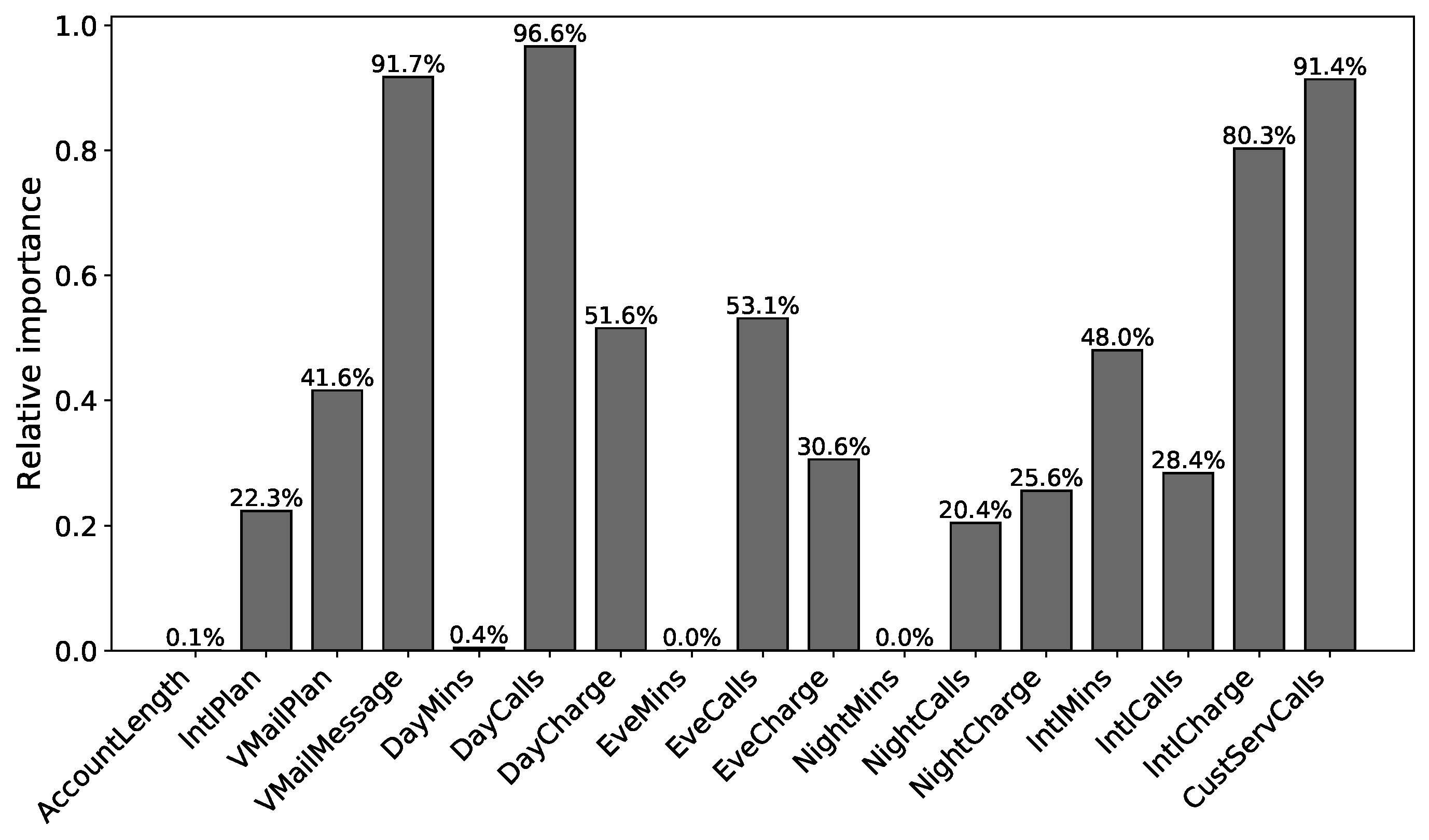
• The model gives insight into the importance of churn factors by assigning a weight for each input feature. This will help decision makers in their strategic plans.

This paper is structured as follows. In Section 2, previous works are reviewed and discussed. In Section 3, the preliminaries of the algorithms utilized in this work are given. Section 4 presents and describes the proposed model in this work. Section 5 describes the datasets used to evaluate the proposed model. The measures used to assess the model are given in Section 6. Then, the experiments and results are presented and discussed in Section 7. Finally, the main outcomes of this work and future work directions are concluded in Section 8.

2. Previous Works

In the last two decades, many machine learning-based models have been proposed for churn prediction in the telecommunication market. These models are varied in type, complexity and the level of interpretability. Different previous works investigated the application of simple or classical machine learning models such as Naïve Bayes, Decision Trees, Artificial Neural Networks (ANN), Support Vector Machines (SVM), and k-Nearest Neighbors (k-NN) [14,15,16,17]; Genetic Programming [18]; and their hybridized forms [19,20,21,22,23]. Most of these works evaluate the performance of the algorithms for churn prediction without significant contribution or modification at the algorithmic level.

Although some of the aforementioned algorithms enjoy powerful generalization performances and other advantages such as high scalability, robustness and good interpretability, they have a major problem when dealing with imbalanced data distribution. This problem is very common in the data of churn customers in the telecommunication market, where the churners are outnumbered by the loyal customers. With such a problem, standard machine learning approaches seek for maximizing the accuracy results for the large classes and ignoring the small ones, which leads to poor generalization performance [24]. Therefore, different types of approaches are proposed for handling the imbalanced data distribution. These approaches can be classified into three main categories: algorithm level approach (internal approach), data level approach (external approach), and ensemble approach [25]. Each of these categories has its own advantages and disadvantages.

In the context of churn prediction in the telecommunication market, there are different examples from the literature on each approach. The internal approach aims at modifying the state-of-the-art algorithms to consider the importance of the rare instances that form the churners class. Zhao et al. [26] presented an example of such work, where they proposed an improved one-class support vector machine for churn prediction based on a highly imbalanced dataset. Their results show that the improved one-class SVM with an RBF kernel function can outperform other traditional approaches such as neural networks, decision trees, and Naïve Bayes.

Another line of research followed the data level approach, which tries to improve the quality of the data at the preprocessing stage before training the classification algorithms. This approach usually modifies the distribution of the data by performing oversampling or undersampling. An example of this approach was presented by Idris et al. [27], where the authors used a PSO-based undersampling technique for churn prediction. In this method, PSO searches for the most informative examples of the majority class, ranks them and then combines them with the minority class to maximize the accuracy of the classification. They selected maximizing AUC as their fitness in combination with k-NN and Random Forest (RF) classifiers. Their results show that the PSO-based method improved the performance of RF and k-NN. Another undersampling method called Neighborhood Cleaning Rules (NCL) is applied for balancing churn data in [28]. NCL considers the quality of the removed data by performing data cleaning rather than data reduction. After applying NCL, a modified version of PSO called Constricted PSO is trained for developing the churn prediction model. The experiments show that NCL significantly improved the coverage rate of the churn class.

Ensemble classifiers are also applied for churn prediction as another approach for tackling the imbalanced class distribution issue in the data. The basic idea of this approach is to combine the decisions of multiple basic classifiers to reach a higher prediction accuracy. AdaBoost, Bagging and Random Forests are the most popular ensemble classifiers. A recent example of this type of approach is presented in [29]. The authors proposed a heterogeneous ensemble model based on stacking. This model was used to obtain initial predictions to be processed along with any discrepancies through a rule-based heuristic technique for final predictions. The experimental results showed that their proposed approach was more efficient in terms of cost than other popular ensemble approaches such as boosting and bagging. Other examples of studies that investigate the application of ensemble algorithms and their variations for churn prediction can be found in [6,30,31,32,33,34].

Based on the conducted review, it can be noticed that Artificial Neural Networks (ANNs) are among the most applied models in the literature for churn prediction. For example, in [35], a Multilayer Perceptron (MLP) neural network approach is proposed to predict customer churn in one of the major Malaysian telecommunication companies. Its results are compared to the results obtained by Multiple Regression Analysis and Logistic Regression Analysis. Based on the obtained results, the authors recommended MLP as a powerful alternative to statistical measures. In [17], the authors compared the performance of MLP with Backpropagation as a learning method to other popular algorithms such as Support vector Machines, Decision Trees and Linear Regression based on a publicly available churn dataset. They used Monte Carlo simulations to tune the best parameters of each algorithm and found that MLP networks and Decision Trees (i.e., C5.0 algorithm) are the best algorithms for their case, while SVM came very close. Similar simple applications of MLP for churn prediction are also introduced in several works (e.g., [16,36]).

Hybrid approaches based on neural networks were also proposed for churn prediction. Tsai and Lu proposed two hybrid models [20] by combining two types of neural networks: MLP ANN and Self-Organizing Maps (SOM). The neural networks are combined in a serialized manner, where the first performs data reduction to eliminate unrepresentative data, and the second is used to develop the final churn prediction model. They tested MLP and SOM as a first step and fixed MLP as a second step. They found that the ANN+ANN approach outperforms the SOM+ANN approach as well as the baseline ANN model.

Nature-inspired algorithms were also applied in different ways to tackle the churn prediction problem. In particular, PSO has shown promising results when applied for churn prediction. In the learning stage, Yu et al. [37] proposed a particle classification optimization for initializing the weights and biases of the backpropagation network for customer churn prediction. Their proposed approach outperforms the classical backpropagation-based neural network. In [28], a modified version of PSO called Constricted PSO is trained for developing the churn prediction model. At the preprocessing stage, Vijaya and Sivasankar [10] proposed variants of PSO to perform feature selection and classification. The results, based on imbalanced data, show that the proposed approaches outperform other common classifiers and hybrid approaches. PSO is also used at the preprocessing stage as an undersampling method in [27].

Although some of the previously mentioned approaches show improvements in terms of prediction accuracy, these improvements come at the price of complexity and interpretability of the model. In other words, most previous works focus on the prediction power of their models, without giving enough attention to the problem of identifying the most informative variables that affect the churn of customers. In contrast, the proposed model in this work aims at producing simple prediction models that can give a relevant weight for each variable. This advantage can significantly help decision makers in forming their strategic plans and designing their marketing campaigns. Moreover, unlike most previous works, which focus on utilizing the classical MLP network with backpropagation network, this work uses RWN to overcome the limitations of the previous approach. RWN has an extremely fast learning process, and is easier to configure. On the other hand, although PSO was applied in different ways for churn prediction, to the best our knowledge, it has not been investigated as a feature weighting approach for this problem.

3. Preliminaries

3.1. Particle Swarm Optimization

PSO is a very popular and well-regarded metaheuristic optimizer that was first developed by Kennedy and Eberhart in 1995 [38]. PSO mimics the movement of the bird swarms for finding food sources. Similar to many other evolutionary and swarm intelligent algorithms, PSO starts by initialing a population of random particles where each particle is considered as a candidate solution. Then, PSO starts iteratively its search process to find the best solution by updating the particles according to a predefined fitness function (also known as cost function). In PSO, the updating mechanism that applies on the particle is controlled by: the current location of the particle itself, the best-so-far location found by the particle, which is known as personal best (pBest), and the best location found by the swarm, which is known as global best (gBest).

For a given specific problem, the positions of the particles are updated using the fitness function to determine their movements (known as velocity) within the search space. The velocity is measured by considering the personal best position and the best position achieved by the particle’s neighbors. Moreover, the movement of the particle is influenced by its inertia, and other constants.

In PSO, the positions of the particles are updated using the following mechanism:

$$X_i(t+1)=X_i(t)+V_i(t+1)$$

(1)

where $X_i$ is the particle position i, t is the current iteration, and $V_i$ is the velocity of particle i. $V_i$ is measured as follows:

$$\begin{array}{c}\hfill V_i(t+1)=W·V_i(t)+r_1·c_1·[pBes{t}_i-X_i(t)]\\ \hfill +r_2·c_2·[gBes{t}_i-X_i(t)]\end{array}$$

(2)

where W is inertia weight, $r_1$ and $r_2$ are random numbers between 0 and 1, $c_1$ and $c_2$ are constant coefficients, $pBes{t}_i$ is the current best position of particle i, and $gBes{t}_i$ is the current best position of the swarm.

3.2. Feedforward Neural Networks

Neural networks are powerful mathematical models that consist of simple preprocessing elements called neurons. The types of neural networks are distinguished by their structure and learning algorithms. In Feed-Forward Neural Networks (FFNN), which are the most commonly used type of neural networks, neurons are distributed over several layers: the input layer, a number of hidden layers and the output layer. In every layer, each neuron is fully connected with the neurons in the proceeding layer.

Every neuron is formed by a summation function and activation function. The first sums the weighted inputs of the neuron as expressed in Equation (3), where ${\omega }_{ij}$ is the connection weight between the input i and neuron j, $b_j$ is the bias term of the neuron, and n is number of inputs. The most commonly used activation function is the sigmoidal function given in Equation (4).

$$S_j=\sum _{i=1}^n{\omega }_{ij}{I}_i+b_j$$

(3)

$$g(S_j)=\frac{1}{1+e^{-S_j}}$$

(4)

The most popular structure of FFNNs is the Single Hidden Layer Feedforward neural network (SLFN). SLFN can be mathematically modeled as follows. For N arbitrary distinct training instances given by ($x_i$,$y_i$), where $x_i={[x_{i1},x_{i2},\dots ,x_{in}]}^T$$\in {\mathbb{R}}^d$ and $y_i={[y_{i1},y_{i2},\dots ,y_{in}]}^T$ $\in {\mathbb{R}}^k$, standard SLFNs with activation function $g(x)$ and m hidden neurons can be mathematically described as in Equation (5):

$$y_i=\sum _{j=1}^m{\beta }_{j}g({\omega }_j·x_i+b_j),i=1,\cdots ,n$$

(5)

where $b_j$ is the threshold of the jth hidden neuron, $w_j={(w_{j1},w_{j2},\cdots ,w_{jd})}^T$ is the weight that connects the ith hidden neuron with input neurons, and ${\beta }_j={({\beta }_{j1},{\beta }_{j2},\cdots ,{\beta }_{jm})}^T$ is the vector of weights to connect the ith hidden neuron to the output neurons.

Different types of learning algorithms in the literature can be used to optimize the connection weights in the neural networks such as the famous backpropagation algorithm. Despite its popularity, backpropagation suffers from major drawbacks such as slow convergence and high probability of being trapped in a local minimum.

3.3. Random Weight Networks

In this work, we adopt the Random Weight Network (RWN) as a fast learning algorithm to overcome the aforementioned problems of backpropagation. RWN was first introduced by Schmidt et al. in 1992 [39] as a learning approach for SLFN. In RWN, the input weights and the biases of the hidden layer are randomly set, then the output weights are analytically determined using the Moore–Penrose generalized inverse. Therefore, unlike gradient-descent methods, RWN needs an iterative process for tuning the connection weights of the network.

RWN can be mathematically modeled as follows. Equation (5) N can be rewritten as Equation (6):

$$H\beta =Y$$

(6)

where

$$\begin{array}{c}\hfill H={\left[\begin{array}{ccc}g({\omega }_1.x_1+b_1)& \dots & g({\omega }_m.x_1+b_m)\\ ⋮& & ⋮\\ g({\omega }_1.x_n+b_1)& \dots & g({\omega }_m.x_n+b_m)\end{array}\right]}_{n\times m}\end{array}$$

(7)

$$\beta =({\beta }_1^T,\dots ,{\beta }_m^T)$$

(8)

and

$$Y=(y_1^T,\dots ,y_n^T)$$

(9)

where H is output matrix of the hidden layer and the ith column of H is the ith hidden output vector of neuron with regard to $x_1,x_2,\dots ,x_n$.

The smallest least-square solution of Equation (6) can be obtained by solving the optimization problem given in Equation (10).

$$\underset{\beta }{min}=∥H\beta -Y∥$$

(10)

$$\widehat{\beta }=H^{†}Y$$

(11)

where $H^{†}={(H{H}^T)}^{-1}H$ is the Moore–Penrose generalized inverse of matrix H.

3.4. Adaptive Synthetic Sampling (ADASYN)

ADASYN [40] is an oversampling method which is based on extending the common popular Synthetic Minority Oversampling Technique (SMOTE) [41]. Following the same technique as SMOTE, ADASYN aims at handling the imbalanced data distribution by synthetically creating new instances from the minority class using linear interpolation between the existing minority class instances. However, ADASYN creates synthetic instances according to the level of difficulty of the minority instances in the classification. That is, more instances are generated from the instances close to the boundary between the classes than in the interior of the minority class, which is easier to classify.

4. Proposed Approach

This section presents the details of the proposed approach for churn prediction, which is based on the use of PSO for feature weighting and optimizing the structure of neural network, simultaneously. The proposed approach iteratively assigns random weights to the input features and evaluates them based on their prediction power. The advantage of this technique is that it automatically identifies the importance of the input features in regard to the problem under investigation. Moreover, the model learns from an oversampled training dataset to overcome the problem of imbalanced data distribution. The oversampling step is performed using an advanced oversampling method called ADASYN. The main components of the model, its formulation issues and its procedure are discussed in the following subsections. Figure 1 shows a high-level description of the proposed approach, which is based on feature weighting, oversampling and neural network. The proposed model will be referred to as ADASYN-wPSO-NN.

4.1. Components

The proposed approach consists of four main components:

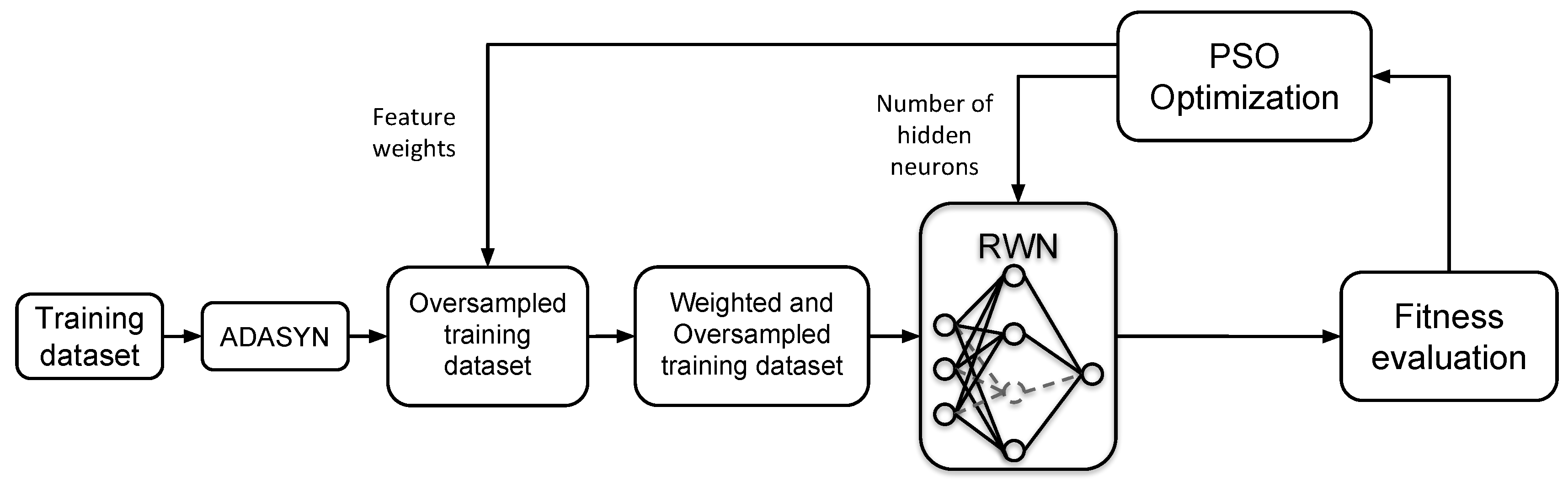
• An oversampling algorithm: The main task of this process is to lessen the problem of the imbalanced class distribution in the dataset by re-sampling the minority class. ADASYN algorithm is selected for this task. It is an improved version of the popular SMOTE algorithm and it has shown its efficiency in various complex imbalanced datasets.
• An optimization algorithm: PSO is utilized to simultaneously optimize the weights of the input features in the training dataset, and the structure of the RWN classifier.
• Inductive algorithm: To evaluate the prediction power of the weighted features, an inductive algorithm, which is a learning classifier, is used. RWN is selected for this task due its simplicity and its extreme learning speed.
• An evaluation measure: To quantify the prediction power of the induction algorithm, an appropriate evaluation measure should be selected. F-measure is used in our developed approach, as it balances between the precision and recall of the class of interest, which is, in our case, the churners class. This point is further explained in the following subsection.

4.2. Formulation

Before applying a metaheuristic optimization algorithm such as PSO for a given problem, two important design issues have to be determined: the representation of the solution of the problem and the measurement used to evaluate the solution. These two issues are discussed and formulated for our proposed approach as follows:

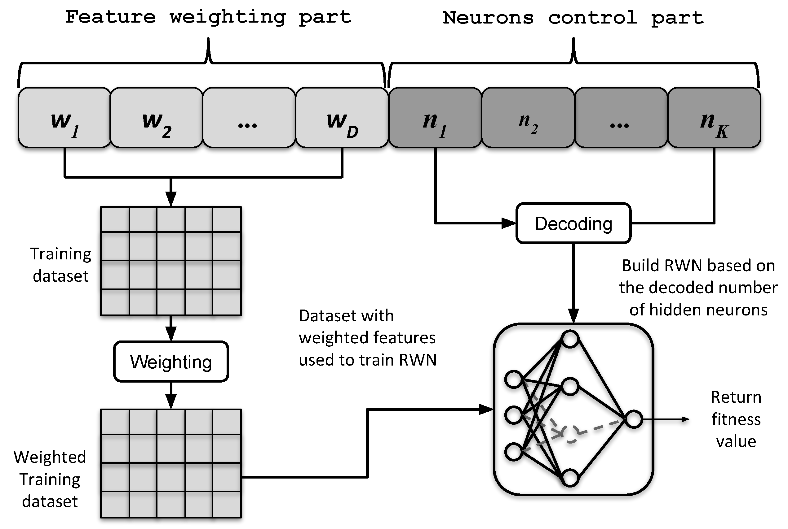
• Solution representation: A particle in PSO represents a candidate solution for the targeted problem. A solution in our case consists of two parts: the weights of the input features and the number of hidden nodes in RWN. In the implementation of the proposed approach, a single individual is encoded as a one-dimensional array of real elements where their values fall between 0 and 1. The first D variables are the weights of their corresponding features, where D is the number of features in the dataset. The second part of the individual consists of K variables to encode the number of hidden nodes. This array can be expressed as follows:

  $$I_i=\left[\begin{array}{cccccccc}{W}_1& W_2& \dots & W_D& h_1& h_2& \dots & h_K\end{array}\right]$$

  (12)
  The part of the hidden neurons is mapped to a binary representation as given in Equation (13), where $f_i$ is the resulted ith element of a sequence of binary flags that encode the number of selected hidden neurons in RWN.

  $$f_i=\left\{\begin{array}{cc}0\hfill & h_i<0.5\hfill \\ 1\hfill & h_i>0.5\hfill \end{array}\right.$$

  (13)
• Fitness evaluation: The merit of the particles/solutions should be evaluated based on a predefined fitness criterion. In this work, the fitness is based on the harmonic mean of precision and recall of the class of interest that is the churn class. This measurement is called F-measure, and it can be calculated as given in Equation (16). The fitness value is calculated based on the predictions of the RWN model that is trained using the weighted features of the training dataset.

  $$F-measure=\frac{2\times Precision\times Recall}{Precision+Recall}$$

  (14)

4.3. Procedure

After formulating the solution representation and determining the fitness function, the processes of the proposed ADASYN-wPSO-NN can be described as follows:

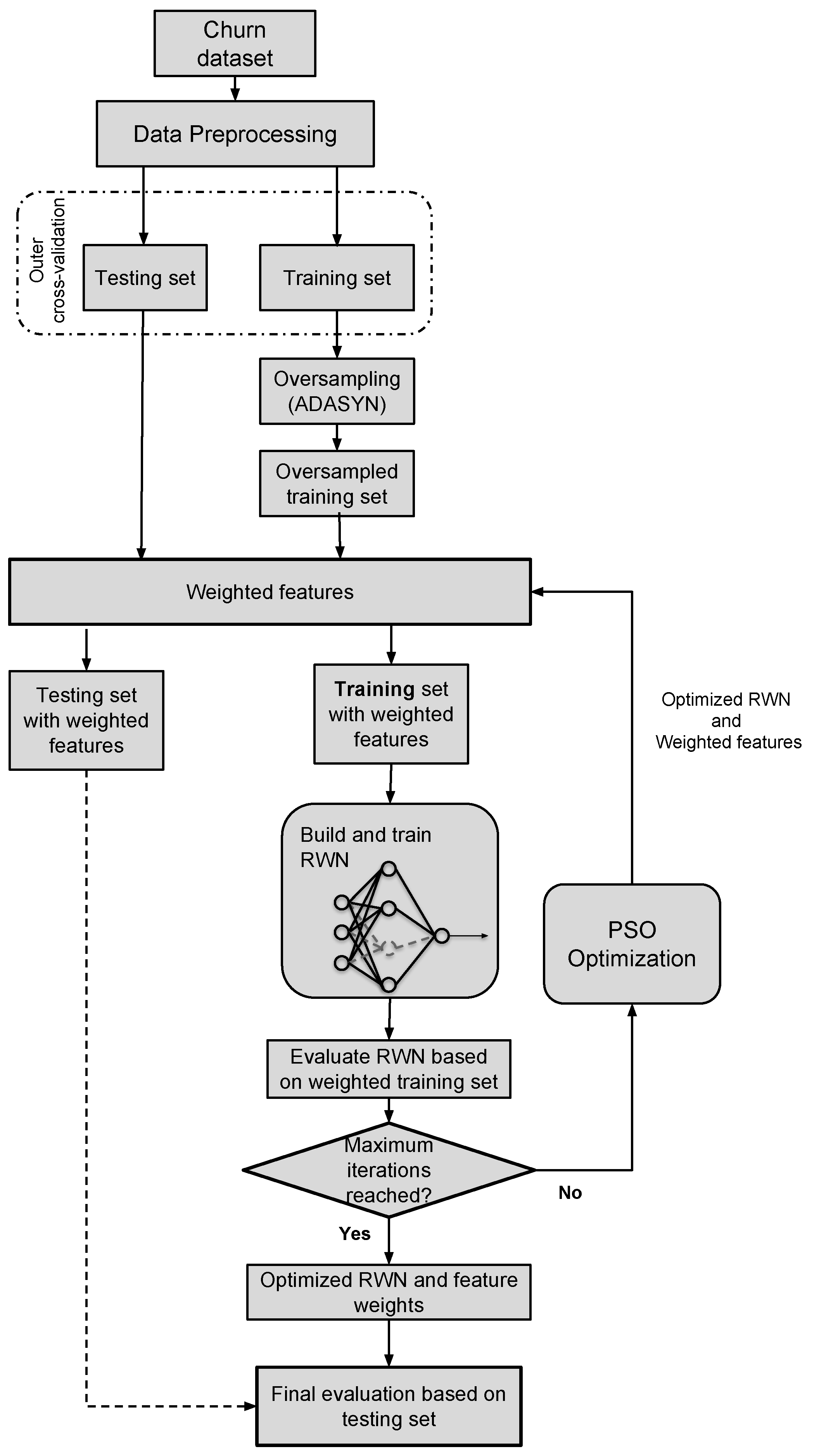
• Initialization: The procedure of ADASYN-wPSO-NN begins by generating a random swarm of particles/candidate solutions where each solution is composed of a set of feature weights and a set of elements that control the number of hidden neurons, as shown in the previous subsection.
• Update: The updating mechanisms of PSO that were described previously in Section 3.1 are utilized at this stage to create a new swarm of particles (possible classification networks).
• Mapping and RWN training: Before calculating the fitness value, the individual is split into two main parts. The first part is used to weight the features of the training data. For example, suppose that we have a set of features such as

  $$F=\{F_1,F_2,\dots ,F_D\}$$

  (15)

  then the training process of RWN is performed based on

  $$\widehat{F}=\{W_1{F}_1,W_2{F}_2,\dots ,W_D{F}_D\}$$

  (16)

  where $W_i$ is the ith element of the weights part and associated with the ith feature. $W_i$ has a real of value between 0 and 1.
  On the other hand, the part that controls the neurons is used to determine the number of hidden nodes in RWN. The resulted RWN is trained based on the weighted training data as explained in Section 3. For example, suppose that we reserve four elements for this part, and there is an individual that has values of [0.2, 0.6, 0.1, 0.7] for these elements, then these values will be rounded as given in Equation (13) to obtain [0, 1, 0, 1]. By converting the resulted binary string to decimal format, five neurons are used in the hidden layer in the RWN.
  The process of feature weighting and determining the number of hidden neurons is illustrated in Figure 2.
• Fitness evaluation: The merit of every generated particle (candidate network) in the swarm is assessed using the F-measure, as given by Equation (16).
• End of procedure: The search process for the best RWN network terminates when a predefined maximum number of iterations is reached. Then, the ADASYN-wPSO-NN model returns the feature weights and the number of hidden nodes required to construct the RWN network that achieved the best fitness quality.
• Testing: For verification, the best constructed RWN network is tested based on a new unseen dataset. Several measurements are used to assess the final network, as explained in Section 6.

The flow of the proposed ADASYN-wPSO-NN approach is illustrated in Figure 3. The figure shows that, by following a cross-validation methodology, the proposed approach starts by splitting the dataset into training and testing and, then, the training part is weighted and used to train the RWN network, while the testing part is kept aside for final evaluation.

5. Datasets Description

5.1. DKD Dataset

This is a dataset of an unknown US mobile operator mentioned in the book “Discovering Knowledge in Data” by Daniel T. Larose [42]. The dataset is (http://dataminingconsultant.com/DMPA_data_sets.zip). It consists of 20 variables (features) and 3333 customers, and a class label that indicates whether a customer churned. The total number of churners is 483, approximately 14.49% of the total customers. The dataset is referred to in this work as DKD dataset. The features of this dataset are listed and described in

Table 1. Description of the features of the DKD dataset.

Feature Name	Description
State	The US state, in which, the customer resides
Account Length	The number of days that this account has been active
Area Code	Area code of the corresponding customer’s phone number
Phone	The remaining seven-digit phone number
Int’l Plan	Whether the customer has an international calling plan (yes/no)
VMail Plan	Whether the customer has a voice mail feature (yes/no)
VMail Message	Presumably, the average number of voice mail messages per month
Day Mins	Total number of calling minutes used during the day
Day Calls	Total number of calls placed during the day
Day Charge	The billed cost of daytime calls
Eve Mins	Total number of calling minutes used during the evening
Eve Calls	Total number of calls placed during the evening
Eve Charge	The billed cost for calls placed during the evening
Night Mins	Total number of calling minutes used during the nighttime
Night Calls	Total number of calls placed during the nighttime
Night Charge	The billed cost for the calls placed during nighttime
Intl Mins	Total number of international calling minutes
Intl Calls	Total number of international calls
Intl Charge	The billed cost for international calls
CustServ Calls	Number of calls placed to Customer Service
Churn	Did the customer leave the service? (true/false)

.

5.2. Local Dataset

This dataset was provided by a major cellular telecommunication company in Jordan. The dataset has 11 variables of randomly selected 5000 customers subscribed to a prepaid service for a time interval of three months. The variables cover outgoing/incoming calls related statistics. The dataset was provided with a class label for each customer indicating whether the customer churned (his subscription was terminated), or the subscription is still active. This dataset is highly imbalanced. There are 381 churners, approximately 7.6% of the total number of customers. A list of the variables along with their description is provided in

Table 2. Description of the features of the local dataset.

Feature Name	Description
3G	Subscriber is provided with 3G service (Yes, No)
Total Consumption	Total monthly fees spent by the customer (calling+SMS) (in JD)
Int’l calling fees	Monthly fees spent by the customer for international calling (in JD)
Int’l MOU	Total minutes of international outgoing calls
Int’l SMS fees	Monthly fees spent by the customer for international SMS (in JD)
Int’l SMS count	Number of monthly international SMS
Local SMS fees	The total monthly local SMS fees spent by the customer (in JD)
Local SMS count	The total number of monthly local SMS
Total MOU	Total minutes of use for all outgoing calls
On net MOU	Total minutes of use for on-net-outgoing calls
Churn	Did the customer leave the service? (true/false)

.

6. Model Evaluation Metrics

The proposed churn prediction model and all the comparative methods in this work are evaluated using a list of evaluation measures that are calculated based on the confusion matrix formed in

Table 3. Confusion matrix.

	Actual
	Churners	nonChurners
Predicted churners	TP	FP
Predicted nonChurners	FN	TN

. The following evaluation measures are used:

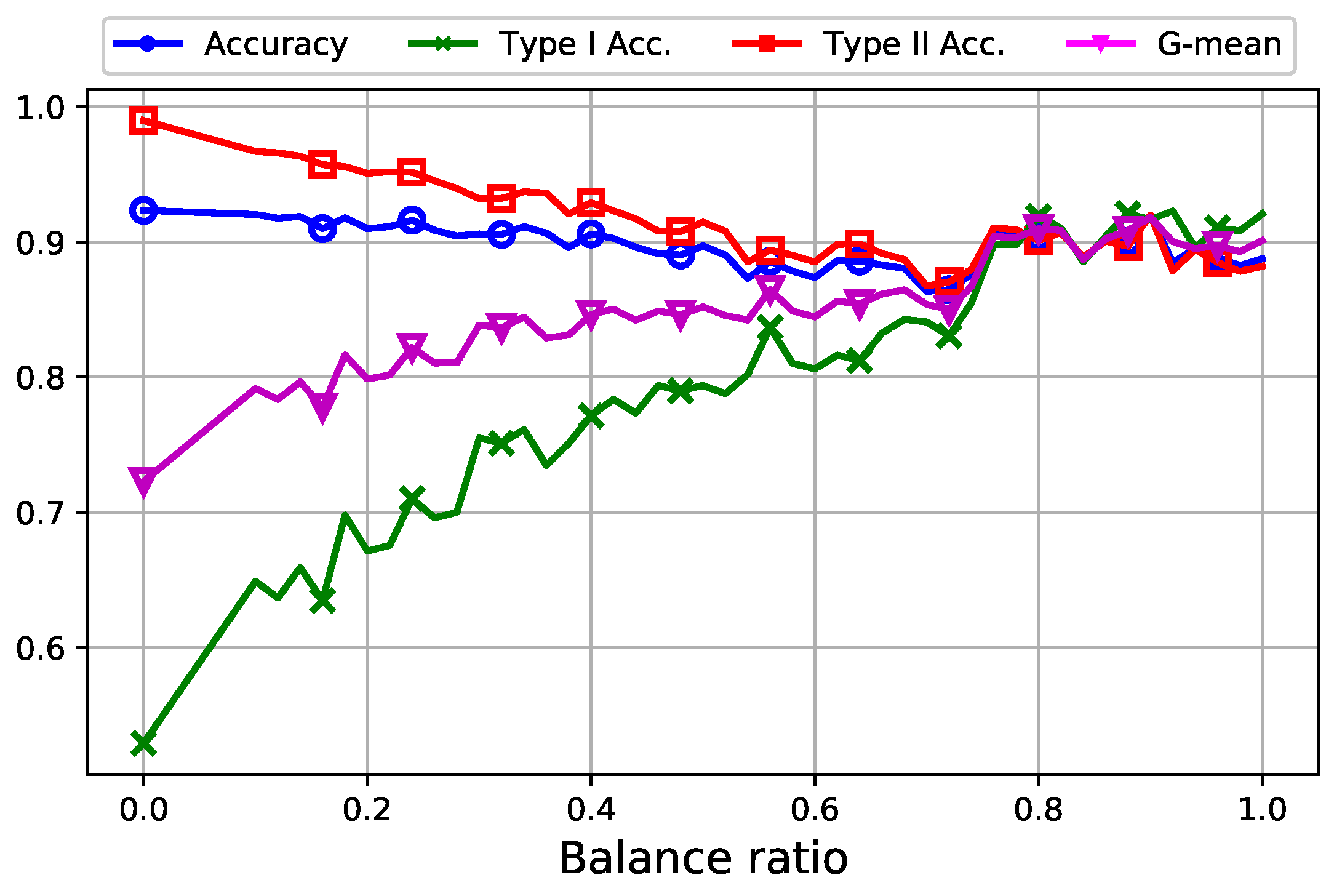
• Accuracy is the ratio of the correct classifications to total number of classifications.

  $$Accuracy=\frac{TN+TP}{TN+TP+FN+FP}$$

  (17)
• Recall is the ratio of relevant instances that are correctly classified to the total amount of relevant instances (i.e., coverage rate). It can be expressed for the churn and non-churn classes by the following equations, respectively.

  $$TypeIAccuracy=\frac{TP}{TP+FN}$$

  (18)

  $$TypeIIAccuracy=\frac{TN}{TN+FP}$$

  (19)
• G-mean is the geometric mean of the recalls of each class and it can be measured by the following equation:

  $$G-mean=\sqrt{TypeIAccuracy\times TypeIIAccuracy}$$

  (20)

7. Experiment and Results

To verify the effectiveness of the proposed model, ADASYN-wPSO-NN was evaluated using the two datasets mentioned in the previous section. For training and testing the proposed model, a 10-fold cross validation was applied. Then, the averages of the evaluation measurements listed in the previous section were calculated. All the experiment of this work were conducted on a server machine with Intel Xeon CPU ES-4609 v4 at 1.70 Ghz (two processors) and 64.0 GB RAM. The proposed algorithm was implemented and tested in MATLAB 2016b software.

For parameters settings, PSO parameters were set based on the effort made in [43,44], where the social and cognitive constants were both set to 1.0, while the inertia constant was set to 0.3. For RWN in ADASYN-wPSO-NN, the range of the number of hidden neurons was set to [1,1024]. The number of the nearest neighbors K in ADASYN was set to 5 [40].

For the comparative methods, the base classifier in the ensembles was the C4.5 decision tree algorithm. The number of iterations was empirically set to 100. In SVM, the grid search was used to set its hyperparameters, where the range of the cost (C) was [0.01,1.0], and the gamma ($\gamma$) was from 0.001 to 1. MLP was applied with one and two hidden layers, where different number of hidden neurons were tested in each layer (5, 10 or 15 neurons). The number that led to the best results is reported. MLP networks were trained with the simple backpropagation learning algorithm. WEKA Environment for Knowledge Analysis version (3.8.1) was used to apply the comparative methods: MLP, SVM, Random Forest, Bagging and AdaBoost [45].

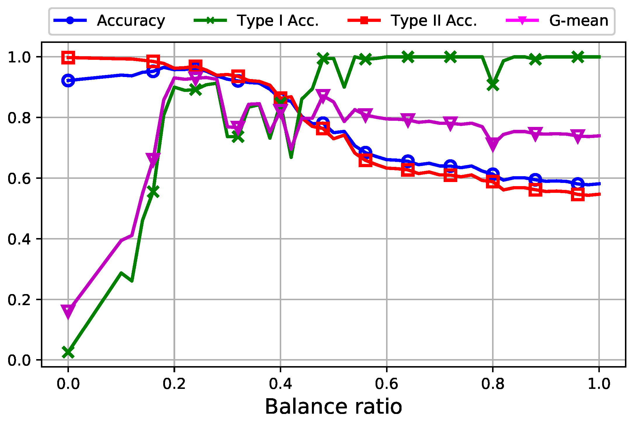
7.1. Analysis of Data Oversampling

At first, the effect of the oversampling component in the proposed model was evaluated. Therefore, we started with testing only the wPSO-NN part without ADASYN, which is denoted as 0% balancing ratio. Then, the ADASYN-wPSO-NN model was tested at different balancing ratios starting from 10% to 100% with a step of 2%. The change of the evaluation measures over the course of increasing the balancing ratio based on KDK and the local datasets is demonstrated in Figure 4 and Figure 5, respectively.

First, it can be noticed in both figures that, without oversampling (i.e. 0% balance ratio), the $TypeIAccuracy$, which denotes the coverage of the churners, is very poor: 52.9% in the case of KDK dataset and 2.5% in the local dataset. This indicates the difficulty that the model faces in handling the imbalance distribution in the datasets and identifying the churners, which form the rare class.

Tracking the change of the measurements by increasing the balance ratio, it can be seen that the $TypeIAccuracy$ and $G-mean$ noticeably increase until a certain point and then both measurements stay steady or slightly decrease. For KDK dataset, the balancing ratio at which the $TypeIAccuracy$ and $G-mean$ are at their maximum is 90%, while for the local dataset, this ratio is 24%. It is also observed that, as the $TypeIAccuracy$ increases, the $TypeIIAccuracy$ of the non-churners decreases. However, this decrement happens at a slighter manner. The same applies for the general accuracy rate. In the KDK dataset, oversampling the dataset with a ratio of 90% increased $TypeIAccuracy$ from 52.9% to 91.6%, however, with a small decrement of $TypeIIAccuracy$ from 98.8% to 92%. For the local dataset, oversampling the dataset with a ratio of 24% increased $TypeIAccuracy$ from 2.5% to 89.2%, but with a small reduction in $TypeIIAccuracy$ from 99.7% to 96.8%. Therefore, significant improvement in the coverage rate of churners can be achieved by ADASYN with the right balancing ratio at a cost of slight decrease in the coverage rate of non-churners.

As explained in Section 4, one of the main features of the proposed ADASYN-wPSO-NN model is that it automatically tunes the required number of hidden nodes in its RWN network. Figure 6 shows the change in the average number of the selected hidden neurons over the course of the iterations for KDK and local datasets at the best balancing ratios. As it can be noticed at the beginning of the iterations, the number of hidden nodes fluctuates and covers a wide range in an attempt to discover the right number of nodes that maximizes the classification accuracy. After 20 neurons, the curves become more stable, which indicates a convergence toward the best number of hidden nodes. Figure 7 shows the convergence curves of ADASYSN-wPSO-NN for KDK and local datasets over the course of iterations.

7.2. Comparison with other Classifiers

The performance of ADASYN-wPSO-NN is compared to other powerful classifiers that are commonly applied in the literature for churn prediction: Support Vector Machine [14,15]; three ensemble classifiers, namely Random Forest, AdaBoost, and Bagging [27,46]; MLP based on two topologies, namely one and two hidden layers, denoted as MLP(I-H-O) and MLP(I-H-H-O), where I, H, and O represent the number of neurons in the input, hidden, and output layers, respectively; and wPSO-NN, which is similar to the proposed model but without oversampling.

Table 4. Evaluation results of ADASYN-wPSO-NN and other comparative methods based on KDK dataset.

	G-mean	Type I Accuracy	Type II Accuracy	Accuracy
ADASYN-PSO-wNN	0.918	0.917	0.920	0.920
PSO-wNN	0.723	0.529	0.990	0.923
Bagging	0.862	0.752	0.987	0.953
AdaBoost	0.863	0.756	0.985	0.952
Random Forest	0.876	0.776	0.989	0.959
Grid-SVM	0.893	0.849	0.941	0.931
MLP(17-10-2)	0.850	0.735	0.982	0.946
MLP(17-10-10-2)	0.849	0.731	0.986	0.949

and

Table 5. Evaluation results of ADASYN-wPSO-NN and other comparative methods based on the local dataset.

	G-mean	Type I Accuracy	Type II Accuracy	Accuracy
ADASYN-PSO-wNN	0.929	0.892	0.968	0.963
PSO-wNN	0.160	0.026	0.998	0.922
Bagging	0.838	0.703	0.998	0.976
AdaBoost	0.841	0.714	0.991	0.970
Random Forest	0.845	0.717	0.995	0.974
Grid-SVM	0	0	0.924	0.924
MLP(10-10-2)	0.493	0.249	0.977	0.9216
MLP(10-10-10-2)	0.281	0.079	0.997	0.927

list the evaluation results of ADASYN-wPSO-NN against all the other comparative methods based on the KDK and local datasets, respectively. Examining the results, it is clear that the ADASYN-wPSO-NN model had the highest coverage rate of churners among all other classifiers in both datasets by achieving $TypeIAccuracy$ of 91.7% and 89.2%, respectively. This high rate was achieved at the cost of slight decrement for $TypeIIAccuracy$. ADASYN-wPSO-NN also had the highest G-mean at values of 0.981 and 0.929, respectively. These superior results give a strong indication that the classifier has a good balance between the two classes, and it is not biased toward either. It is also worth mentioning that the general accuracy rate does not give a proper indication on the performance and it could be misleading. This is because, although a classifier can be highly biased toward the majority class, it can still have a high accuracy rate. In both tables, although all algorithms obtained very competitive accuracy rates, they have noticeable differences at the level of coverage rates (Type I and Type II accuracies) and G-mean values.

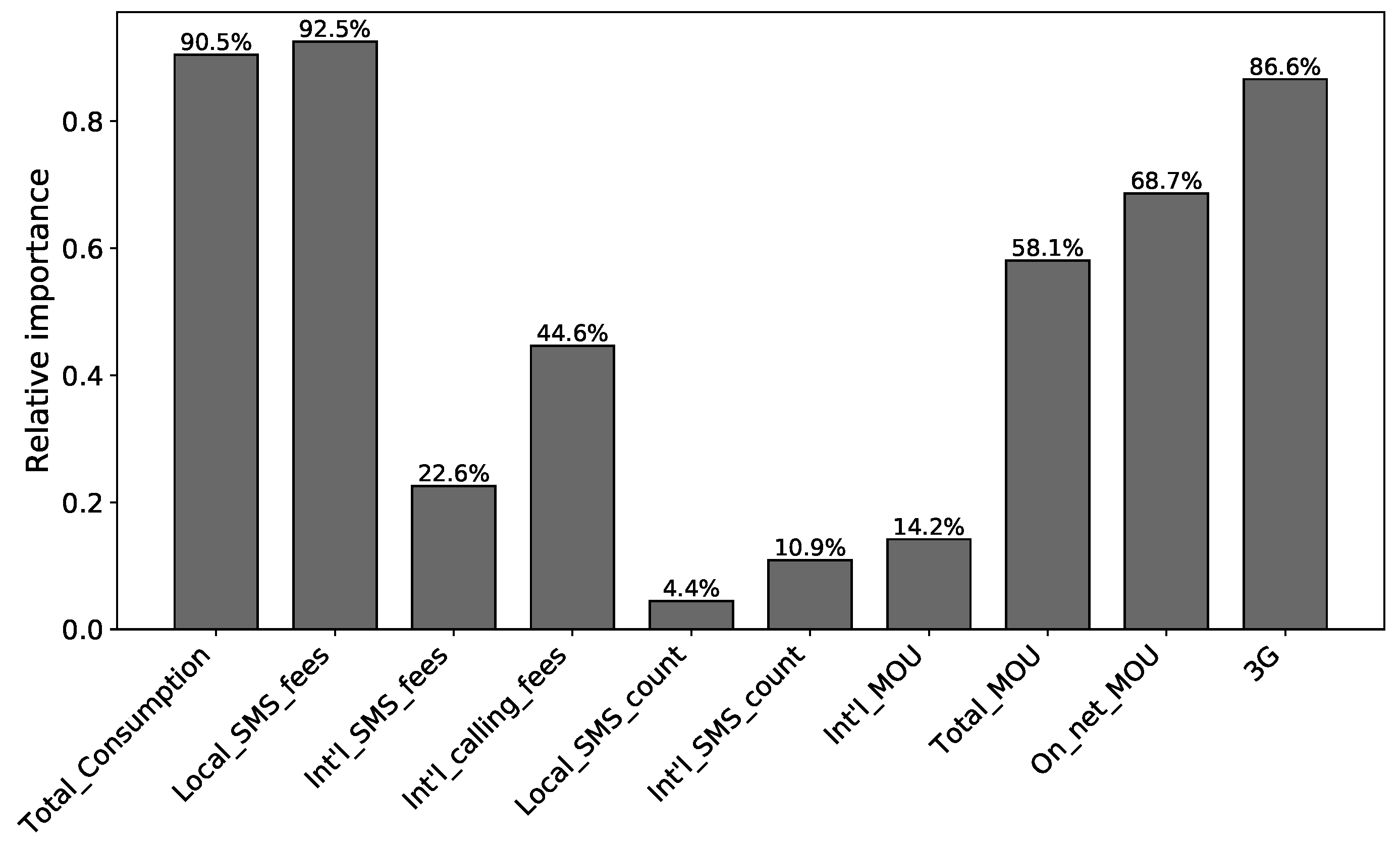
7.3. Relative Importance of Churn Features

Another important feature of ADASYN-wPSO-NN is the automatic identification of the important features in the classification process. Over the course of iterations, PSO tries to optimize the weights of the features to reach the best fitness quality. Therefore, these weights can be interpreted as important factors for their corresponding features.

Figure 8 shows the average weights obtained by the model for the features of KDK dataset. It can be seen that the features that have the highest weights are Day Calls (96.6%), VMail Message (91.7%), CustServ Calls (91.4%) and Intl Charge (80.3%). In general, it can also be observed that the weights for the day calls and their charges are much higher than those for the evening and night calls and charges. This can give a strong indication for decision makers to reconsider their strategic plans regarding the day calls and their charges. It is rather interesting to see that the number of calls placed to customer service is one of the highest weighted features. This feature can be strongly related to the quality of customer service provided by the company.

Figure 9 shows the weights assigned by the model for the features of the local dataset. The highest weighted features are Local SMS fees (92.5%), Total Consumption (90.5%), 3G (86.6%), On net MOU (68.7%) and Total MOU (58.1%). In general, it is noticed that the plans related to the local SMS and 3G subscriptions are the most significant factors in this dataset at the time of its collection.

Overall, giving insight into the importance of each feature as in the previous two cases can help decision makers in understanding the real factors that affect customer churn in a highly dynamic and complex market. This can effectively contribute in implementing efficient systems to monitor the factors that affect customers’ decisions about churn, and consequently controlling and reducing its impact as a proactive approach. For example, the customers that are identified by the developed model as churners can be directly targeted by the company, which can survey their satisfaction about some services related to the features that have the highest weights (i.e., the quality of the 3G service, satisfaction of customer service calls, or prices of international calls). Based on this information, discounts and special offers can be given to those customers, or the quality of service can be improved if the problem is related to other factors such as the quality of coverage or customer service calls.

8. Conclusions

In this work, a new hybrid model that combines Particle Swarm Optimization with Random Weight Network is proposed. The new model targets the problem of churn prediction in telecommunication companies. In the developed model, PSO is used to simultaneously optimize the weights of the input features and to tune the structure of the RWN network. In addition, an advanced oversampling method is used to improve the learning from the imbalanced churn datasets. The experimental results based on two datasets show that the model can significantly improve the coverage rate of churn customers in comparison with other powerful state-of-the-art classifiers. The automatic optimization of the network structure eliminated the effort needed for setting the best number of hidden neurons. Another important feature of the proposed model is that it automatically optimizes the weights of the input features, which reflect the importance of their corresponding features in the identification process. It is expected that this feature will help practitioners and decision makers to assess the role of the identified important features in designing their marketing campaigns. This can help in implementing systems to monitor the factors that affect the churn of customers, and consequently controlling and reducing their impact.

For future work, the efficiency of the proposed feature weighting and classification approach can be investigated based on other types of oversampling and undersampling methods. Moreover, the developed model will be used to investigate other common business applications such as credit risk analysis and direct marketing problems.

References

1. Wei, C.P.; Chiu, I.T. Turning telecommunications call details to churn prediction: A data mining approach. Expert Syst. Appl. 2002, 23, 103–112. [Google Scholar] [CrossRef]
2. Hadden, J.; Tiwari, A.; Roy, R.; Ruta, D. Computer assisted customer churn management: State-of-the-art and future trends. Comput. Oper. Res. 2007, 34, 2902–2917. [Google Scholar] [CrossRef]
3. Keramati, A.; Ardabili, S.M. Churn analysis for an Iranian mobile operator. Telecommun. Policy 2011, 35, 344–356. [Google Scholar] [CrossRef]
4. Baesens, B.; Verstraeten, G.; Van den Poel, D.; Egmont-Petersen, M.; Van Kenhove, P.; Vanthienen, J. Bayesian network classifiers for identifying the slope of the customer lifecycle of long-life customers. Eur. J. Oper. Res. 2004, 156, 508–523. [Google Scholar] [CrossRef] [Green Version]
5. García, D.L.; Nebot, À.; Vellido, A. Intelligent data analysis approaches to churn as a business problem: A survey. Knowl. Inf. Syst. 2017, 51, 719–774. [Google Scholar] [CrossRef]
6. Mozer, M.C.; Wolniewicz, R.; Grimes, D.B.; Johnson, E.; Kaushansky, H. Predicting subscriber dissatisfaction and improving retention in the wireless telecommunications industry. IEEE Trans. Neural Netw. 2000, 11, 690–696. [Google Scholar] [CrossRef] [PubMed]
7. Li, H.; Yang, D.; Yang, L.; Lu, Y.; Lin, X. Supervised Massive Data Analysis for Telecommunication Customer Churn Prediction. In Proceedings of the 2016 IEEE International Conferences on Big Data and Cloud Computing (BDCloud), Social Computing and Networking (SocialCom), Sustainable Computing and Communications (SustainCom) (BDCloud-SocialCom-SustainCom), Atlanta, GA, USA, 8–10 October 2016; pp. 163–169. [Google Scholar]
8. Ngai, E.; Xiu, L.; Chau, D. Application of data mining techniques in customer relationship management: A literature review and classification. Expert Syst. Appl. 2009, 36, 2592–2602. [Google Scholar] [CrossRef]
9. Idris, A.; Khan, A. Churn Prediction System for Telecom using Filter–Wrapper and Ensemble Classification. Comput. J. 2016, 60, 410–430. [Google Scholar] [CrossRef]
10. Vijaya, J.; Sivasankar, E. An efficient system for customer churn prediction through particle swarm optimization based feature selection model with simulated annealing. Cluster Comput. 2017. [Google Scholar] [CrossRef]
11. Huang, G.B.; Zhu, Q.Y.; Siew, C.K. Extreme learning machine: Theory and applications. Neurocomputing 2006, 70, 489–501. [Google Scholar] [CrossRef] [Green Version]
12. Han, F.; Yao, H.F.; Ling, Q.H. An improved evolutionary extreme learning machine based on particle swarm optimization. Neurocomputing 2013, 116, 87–93. [Google Scholar] [CrossRef]
13. Ding, S.; Xu, X.; Nie, R. Extreme learning machine and its applications. Neural Comput. Appl. 2014, 25, 549–556. [Google Scholar] [CrossRef]
14. Xia, G.; Jin, W. Model of customer churn prediction on support vector machine. Syst. Eng. Theory Pract. 2008, 28, 71–77. [Google Scholar] [CrossRef]
15. Rodan, A.; Faris, H.; Alsakran, J.; Al-Kadi, O. A Support Vector Machine Approach for Churn Prediction in Telecom Industry. Int. J. Inf. 2014, 17, 3961–3970. [Google Scholar]
16. Adwan, O.; Faris, H.; Jaradat, K.; Harfoushi, O.; Ghatasheh, N. Predicting customer churn in telecom industry using multilayer preceptron neural networks: Modeling and analysis. Life Sci. J. 2014, 11, 75–81. [Google Scholar]
17. Vafeiadis, T.; Diamantaras, K.I.; Sarigiannidis, G.; Chatzisavvas, K.C. A comparison of machine learning techniques for customer churn prediction. Simul. Model. Pract. Theory 2015, 55, 1–9. [Google Scholar] [CrossRef]
18. Khan, I.; Usman, I.; Usman, T.; Rehman, G.U.; Rehman, A.U. Intelligent churn prediction for telecommunication industry. Int. J. Innov. Appl. Stud. 2013, 4, 165–170. [Google Scholar]
19. Keramati, A.; Jafari-Marandi, R.; Aliannejadi, M.; Ahmadian, I.; Mozaffari, M.; Abbasi, U. Improved churn prediction in telecommunication industry using data mining techniques. Appl. Soft Comput. 2014, 24, 994–1012. [Google Scholar] [CrossRef]
20. Tsai, C.F.; Lu, Y.H. Customer churn prediction by hybrid neural networks. Expert Syst. Appl. 2009, 36, 12547–12553. [Google Scholar] [CrossRef]
21. Rodan, A.; Faris, H. Echo state network with SVM-readout for customer churn prediction. In Proceedings of the 2015 IEEE Jordan Conference on Applied Electrical Engineering and Computing Technologies (AEECT), The Dead Sea, Jordan, 3–5 November 2015; pp. 1–5. [Google Scholar]
22. Faris, H.; Al-Shboul, B.; Ghatasheh, N. A genetic programming based framework for churn prediction in telecommunication industry. In Proceedings of the International Conference on Computational Collective Intelligence, Madrid, Spain, 21–23 September 2015; pp. 353–362. [Google Scholar]
23. Al-Shboul, B.; Faris, H.; Ghatasheh, N. Initializing genetic programming using fuzzy clustering and its application in churn prediction in the telecom industry. Malays. J. Comput. Sci. 2015, 28, 213–220. [Google Scholar] [CrossRef]
24. Galar, M.; Fernandez, A.; Barrenechea, E.; Bustince, H.; Herrera, F. A review on ensembles for the class imbalance problem: Bagging-, boosting-, and hybrid-based approaches. IEEE Trans. Syst. Man Cybern. C 2012, 42, 463–484. [Google Scholar] [CrossRef]
25. Zhu, B.; Baesens, B.; vanden Broucke, S.K. An empirical comparison of techniques for the class imbalance problem in churn prediction. Inf. Sci. 2017, 408, 84–99. [Google Scholar] [CrossRef]
26. Zhao, Y.; Li, B.; Li, X.; Liu, W.; Ren, S. Customer churn prediction using improved one-class support vector machine. In Proceedings of the International Conference on Advanced Data Mining and Applications, ADMA 2005, Wuhan, China, 22–24 July 2005; pp. 300–306. [Google Scholar]
27. Idris, A.; Rizwan, M.; Khan, A. Churn prediction in telecom using Random Forest and PSO based data balancing in combination with various feature selection strategies. Comput. Electr. Eng. 2012, 38, 1808–1819. [Google Scholar] [CrossRef]
28. Faris, H. Neighborhood Cleaning Rules and Particle Swarm Optimization for Predicting Customer Churn Behavior in Telecom Industry. Int. J. Adv. Sci. Technol. 2014, 68, 11–22. [Google Scholar] [CrossRef]
29. Ahmed, A.A.; Maheswari, D. An enhanced ensemble classifier for telecom churn prediction using cost based uplift modelling. Int. J. Inf. Technol. 2018. [Google Scholar] [CrossRef]
30. Idris, A.; Khan, A.; Lee, Y.S. Genetic Programming and Adaboosting based churn prediction for Telecom. In Proceedings of the IEEE International Conference on Systems, Man, and Cybernetics, SMC 2012, Seoul, Korea, 14–17 October 2012; pp. 1328–1332. [Google Scholar]
31. Lu, N.; Lin, H.; Lu, J.; Zhang, G. A Customer Churn Prediction Model in Telecom Industry Using Boosting. IEEE Trans. Ind. Inf. 2014, 10, 1659–1665. [Google Scholar] [CrossRef]
32. Bock, K.W.D.; den Poel, D.V. An empirical evaluation of rotation-based ensemble classifiers for customer churn prediction. Expert Syst. Appl. 2011, 38, 12293–12301. [Google Scholar] [CrossRef]
33. Xie, Y.; Li, X.; Ngai, E.; Ying, W. Customer churn prediction using improved balanced random forests. Expert Syst. Appl. 2009, 36, 5445–5449. [Google Scholar] [CrossRef]
34. Rodan, A.; Fayyoumi, A.; Faris, H.; Alsakran, J.; Al-Kadi, O. Negative correlation learning for customer churn prediction: A comparison study. Sci. World J. 2015, 2015, 473283. [Google Scholar] [CrossRef] [PubMed]
35. Ismail, M.R.; Awang, M.K.; Rahman, M.N.A.; Makhtar, M. A multi-layer perceptron approach for customer churn prediction. Int. J. Multimed. Ubiquitous Eng. 2015, 10, 213–222. [Google Scholar] [CrossRef]
36. Sharma, A.; Panigrahi, D.; Kumar, P. A Neural Network based Approach for Predicting Customer Churn in Cellular Network Services. Int. J. Comput. Appl. 2011, 27, 26–31. [Google Scholar] [CrossRef]
37. Yu, R.; An, X.; Jin, B.; Shi, J.; Move, O.A.; Liu, Y. Particle classification optimization-based BP network for telecommunication customer churn prediction. Neural Comput. Appl. 2018, 29, 707–720. [Google Scholar] [CrossRef]
38. Kennedy, J.; Eberhart, R.C. Particle Swarm Optimization. In Proceedings of the IEEE International Conference on Neural Networks, Piscataway, NJ, USA, 27 November–1 December 1995; pp. 1942–1948. [Google Scholar]
39. Schmidt, W.F.; Kraaijveld, M.A.; Duin, R.P. Feedforward neural networks with random weights. In Proceedings of the 11th IAPR International Conference on Pattern Recognition, Vol. II. Conference B: Pattern Recognition Methodology and Systems, The Hague, The Netherlands, 30 August–3 September 1992; pp. 1–4. [Google Scholar]
40. He, H.; Bai, Y.; Garcia, E.A.; Li, S. ADASYN: Adaptive synthetic sampling approach for imbalanced learning. In Proceedings of the IEEE International Joint Conference on Neural Networks, IJCNN 2008, Hong Kong, China, 1–6 June 2008; pp. 1322–1328. [Google Scholar]
41. Chawla, N.V.; Bowyer, K.W.; Hall, L.O.; Kegelmeyer, W.P. SMOTE: Synthetic minority over-sampling technique. J. Artif. Intell. Res. 2002, 16, 321–357. [Google Scholar] [CrossRef]
42. Larose, D.T.; Larose, C.D. Discovering Knowledge in Data: An Introduction to Data Mining; John Wiley & Sons: New York, NY, USA, 2014. [Google Scholar]
43. Simon, D. Biogeography-based optimization. IEEE Trans. Evol. Comput. 2008, 12, 702–713. [Google Scholar] [CrossRef]
44. Mirjalili, S.; Mirjalili, S.M.; Lewis, A. Let a biogeography-based optimizer train your multi-layer perceptron. Inf. Sci. 2014, 269, 188–209. [Google Scholar] [CrossRef]
45. Hall, M.; Frank, E.; Holmes, G.; Pfahringer, B.; Reutemann, P.; Witten, I.H. The WEKA data mining software: an update. ACM SIGKDD Explor. Newsl. 2009, 11, 10–18. [Google Scholar] [CrossRef]
46. Lemmens, A.; Croux, C. Bagging and boosting classification trees to predict churn. J. Mark. Res. 2006, 43, 276–286. [Google Scholar] [CrossRef]
Figure 1. Flow chart of the main processes of the proposed ADASYN-wPSO-NN approach.
Information 09 00288 g001
Figure 2. Solution representation in ADASYN-wPSO-NN.
Information 09 00288 g002
Figure 3. Proposed approach for churn prediction.
Information 09 00288 g003
Figure 4. Effect of balance ratio on the Accuracy, Type I Accuracy, Type II accuracy and G-mean based on KDK dataset.
Information 09 00288 g004
Figure 5. Effect of balance ratio on the Accuracy, Type I Accuracy, Type II Accuracy and G-mean based on the local dataset.
Information 09 00288 g005
Figure 6. Average number of neurons for KDK and local datasets over the course of iterations.
Information 09 00288 g006
Figure 7. Convergence curves ADASYSN-PSO-NN for KDK and local datasets over the course of iterations.
Information 09 00288 g007
Figure 8. Relative importance of features for KDK dataset.
Information 09 00288 g008
Figure 9. Relative importance of features for the local dataset.
Information 09 00288 g009