Performance Analysis of Honeypot with Petri Nets

Abstract

As one of the active defense technologies, the honeypot deceives the latent intruders to interact with the imitated systems or networks deployed with security mechanisms. Its modeling and performance analysis have not been well studied. In this paper, we propose a honeypot performance evaluation scheme based on Stochastic Petri Nets (SPN). We firstly set up performance evaluation models for three types of defense scenarios (i.e., firewall; firewall and Intrusion Detection System (IDS); firewall, IDS and honeypot) based on SPN. We then theoretically analyze the SPN models by constructing Markov Chains (MC), which are isomorphic to the models. With the steady state probabilities based on the MC, the system performance evaluation is done with theoretical inference. Finally, we implement the proposed three SPN models on the PIPE platform. Five parameters are applied to compare and evaluate the performance of the proposed SPN models. The analysis of the probability and delay of three scenarios shows that the simulation results validate the effectiveness in security enhancement of the honeypot under the SPN models.

1. Introduction

Internet security becomes severely important as more and more applications are developed based on the Internet, which require security guarantee. Since the attacker always behaves before the defender, it can gain the asymmetric advantage over the latter. Thus, it is necessary to design effective approaches to make the defender operate more efficiently. Different from the passive security techniques, such as firewalls [1] and the Intrusion Prevention and Detection Systems (IPDS), the honeypot or honeynet [2,3,4] is intended to defend proactively against attackers. Specifically, the functionality of the honeypot is to deceive the attackers to disrupt the imitated networks, systems or services, protecting the real ones.

Ideally, the attackers are not aware of the deployment of the honeypot, which may lead them to spend much time and energy interacting with the fake services or systems. The honeypot is able to record and analyze an attacker’s behavioral traces, which allows the security administrators to understand the behaviors of other attackers and take appropriate countermeasures. Thus, the honeypot is able to detect the unknown attacks with a very low false positive rate. However, one of the honeypot’s drawbacks lies in its own distinctive characteristics. Some powerful intruders can make use of such characteristics to identify the honeypot, based on which they can even compromise the system.

The researchers have given non-trivial effort to improving the security of the honeypot, which will be discussed in the related work in detail. At the same time, the problem about whether it is worth deploying a honeypot in a given network or system has not been well studied. This motivates us to evaluate and examine the performance of the honeypot in a quantitative way. In this paper, we propose to use Stochastic Petri Nets (SPN) [5,6] to model and analyze three network scenarios: the one protected by a firewall, the one protected by both a firewall and IDS [7] and the one deployed with a firewall, IDS and honeynet. Then, we evaluate the performance of the honeypot based on the three corresponding SPN models.

The main contributions of this paper are summarized as follows:

• We propose three scenarios of the system defense mechanism with firewall, firewall + IDS and firewall+ IDS + honeypot, respectively;
• We propose to construct and analyze the SPN models for the three defense scenarios;
• We conduct extensive simulations to validate the effectiveness of honeypot with the SPN models.

The rest of this paper is organized as follows. In Section 2, we discuss the related work. In Section 3, three network scenarios with different security mechanisms are proposed. Section 4 presents the SPN models of the three scenarios with the theoretical analysis. In Section 5, we conduct the performance evaluation. This paper is finally concluded in Section 6.

2. Related Work

During the last decade, various viruses, worms, Trojan horses and malicious codes have puzzled the Internet. Many solutions have been proposed to solve these problems. However, most of the traditional countermeasures, such as firewall and Intrusion Detection Systems (IDS), are passive in nature. The adversaries can attack the conspicuous server at any time and any place. The honeypot has been proposed to act as a trap for the adversaries. It can disturb and confuse the intruders. Thus, the honeypot is considered as an active mechanism for the defenders.

With the scale of the Internet being much bigger and the related technologies being more complex, how to model them and evaluate their performance becomes a significant problem. Researchers have conducted much works on modeling and estimating the performance of the systems with Petri nets in information security.

Mixia et al. [8] presented the system architecture of the network security situation and modeled it with the Colored Petri Nets (CPN) in order to analyze the network security in the view of the system. Hicham et al. [9] proposed a novel approach to detect network security conflicts more generically and specified it with CPN to perform automatic conflict analysis. In [10], a model of Address Resolution Protocol (ARP) spoofing with Petri nets was proposed to validate the feasibility of ARP spoofing. Hwang et al. [11] described the inference rules of computer forensics with Fuzzy Petri Nets (FPN). They extracted and analyzed the collected data from the compromised systems to infer the intrusion information.

Aliannezhadi et al. [12] presented the architecture for web service firewall to protect web security and developed a formal CPN model of access control of the proposed web service firewall architecture. The CPN model of access control was proven to be effective with the simulation results.

Dolgikh et al. used CPN as the backbone of the proposed approach to define the functionality of interest as behavior signatures and to serve as the mechanism for the signature detection in IDS [13]. With Petri nets, Voron et al. [14] described a formal reference behavior model of the proposed novel approach that automatically generates host-based IDS from program sources. Balaz et al. [15] proposed a new IDS architecture based on partially ordered events and a novel detection method that matches the intrusion signature with Petri nets. Toktabayev et al. [16] proposed the IDS based on obfuscation-resilient behavior with CPN describing specific malicious functionality. Nykodym et al. [17] improved the IDS proposed in [16]. They constructed a functional model with CPN that tracks how to access and modify kernel objects.

In [18], an advanced model of the Intrusion Tolerance System (ITS) was proposed, in which the performance of the model with SPN and the Markov process was evaluated. The simulation results showed that the system was secure and efficient. Wang et al. [19] constructed the models of three types of ITS with Generalized Stochastic Petri Nets (GSPN). They analyzed and compared the three kinds of ITS models. The numerical results showed the availability of the three kinds of systems. Yang et al. [20] presented a hybrid IDS based on protocol analysis and detection tree algorithms. They estimated the performance of the proposed system with the GSPN model. Shi et al. [21] proposed a performance evaluation model of a service hopping system with SPN. They inferred and analyzed some parameters to estimate the model’s performance, validating the effectiveness of synchronous delay and data transfer efficiency.

Teo et al. [22] proposed a security framework called Jeponica, with a honeypot as an active entity to detect and deal with the unknown attacks dynamically. They described the model of the framework proposed with CPN to discover a uniform message exchange format among the entities. The results showed that the framework could work effectively.

Besides, there are some other works related to Petri nets. By combining a regular Petri nets with fuzzy rules, a software system model called Intelligent Petri Net (I-PN) was proposed [23], in which the runtime environment and system behavior can be modeled. I-PN features a self-adaption ability. In [24], Petri nets were used for the physiochemical model, which was related to EGFR-Ras-MAPK. Siphon and proteins were involved in identifying targets for multi-component therapies in signaling pathways. Wiśniewski et al. [25] used interpreted Petri nets to describe a concurrent control system. A prototyping technique of the system was proposed, dominating in polynomial time.

However, the aforementioned works are almost related to intrusion detection, web service firewall, ARP spoofing and system architecture in network security. In this paper, we focus on the combination of Petri nets [26] and honeypot. Only in [22], the honeypot was used as a component of the proposed framework, and CPN was involved, which is different from SPN. Therefore, as far as we know, there is no work related to both the honeypot and SPN. Such a scheme is proposed in this paper to analyze the performance of honeypot.

3. Network Scenarios

To compare and analyze the performance of the honeypot, we propose three scenarios of a defense mechanism in computer networks.

In Defense Scenario I, only the firewall is adopted in the defense mechanism, as shown in Figure 1. When the intruder attempts to attack the protected system, it will trigger the defense mechanism. During the defense process, the firewall can obtain rules from the rule database to filter the data sent by the intruder. Once there is a rule that matches the data feature, the firewall will drop the data and log it. As the first line of defense, the firewall protects our system or network from intruders and safeguards our data from attack. However, the conventional firewall is designed as a sequence of rules that suffers from three types of major problems: the consistency problem, the completeness problem and the compactness problem [27]. The firewall can rarely identify types of attacks or attacks on allowed services. Therefore, it is easy for the attackers to cross the firewall.

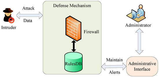
Figure 1. Defense Scenario I with firewall only.

In Defense Scenario II, the IDS will be added into the defense mechanism based on that of the Defense Scenario I, as shown in Figure 2. When the firewall cannot find any rule from its rules database that matches the feature, the data will be delivered to the IDS for detection. The IDS will identify whether the data are legitimate or not based on the signature database of IDS. If so, the IDS will deal with the malicious data. Compared with the function of a firewall, the intrusion detection system is designed as the second line of defense to report corresponding alarms and take immediate action on the intrusions [28]. However, if the network packets are transferred through SSL or VPN, the intrusion detection behavior is hard to detect, and the intrusion detection system will have a lower detection rate and high false negative rate.

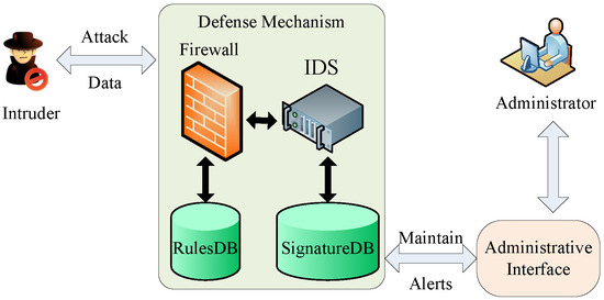
Figure 2. Defense Scenario II with firewall and the Intrusion Detection System (IDS).

In Defense Scenario III, the honeypot is deployed based on the defense mechanism of Defense Scenario II, as shown in Figure 3. If the intruder does not identify the honeypot, it will spend a large amount of time and resource interacting with the imitated services or systems. Accordingly, it will be difficult for the intruder to attack the real system due to its limited remaining energy. In this scenario, the honeypot can be thought as the last line of defense in the network and a supplement to the existing IDS. In the actual deployment of the application, these three technologies complement and benefit one another.

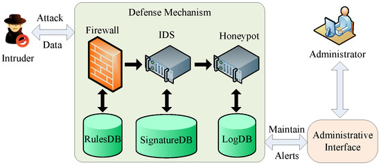
Figure 3. Defense Scenario III with firewall, IDS and honeypot.

Obviously, the firewall and IDS are relatively passive in dealing with some unknown attacks launched by the intruders since they do not own the rules or features of the anomaly. However, the honeypot can actively deceive the intruders to interact with it.

4. SPN-Based Modeling and Analysis

4.1. Stochastic Petri Nets

The SPN model is basically composed of three components: places, transitions and arcs. The places represent the states or resource of the system. The transitions represent the events that enable the system’s state transfer. The arcs illustrate the relationship between the places and transitions.

How can we estimate the performance of a system? Here, we give a sample to illustrate it.

Firstly, we need to construct the performance evaluation model of the target system. That depends on the concrete system you want to analyze. Therefore, we directly give a sample model as shown in Figure 4.

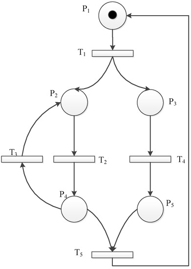
Figure 4. A simple sample of the Stochastic Petri Nets (SPN) model.

Secondly, we can construct the Markov Chain (MC) that is isomorphic to the SPN model. At first, we can easily get the reachable graph of the SPN model (as shown in Figure 5). Then, we assume the transition firing rate average is $\lambda =\{{\lambda }_1,{\lambda }_2,{\lambda }_3,{\lambda }_4,{\lambda }_5\}$. Lastly, we get the MC by replacing the transition $t_i$ with the corresponding ${\lambda }_i$. The reachable markings’ set and the MC of the simple SPN model above are shown in Table 1 and Figure 6.

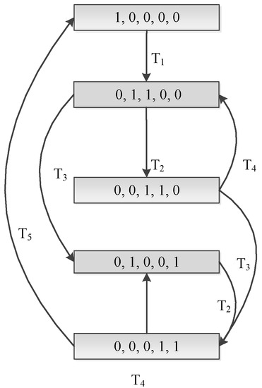
Figure 5. The reachable graph of the sample.

Table 1. Reachable markings’ set of the sample.

	${\mathit{P}}_1$	${\mathit{P}}_2$	${\mathit{P}}_3$	${\mathit{P}}_4$	${\mathit{P}}_5$
$M_1$	1	0	0	0	0
$M_2$	0	1	1	0	0
$M_3$	0	0	1	1	0
$M_4$	0	1	0	0	1
$M_5$	0	0	0	1	1

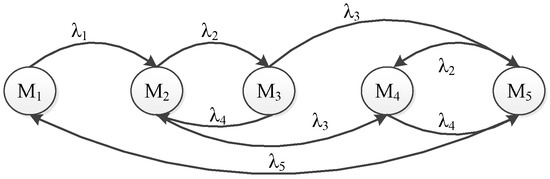
Figure 6. The reachable graph of the sample.

Thirdly, we can work on the system performance evaluation with the steady state probability based on the MC. There are some formulas that help the theoretical inference. They are as follows.

We assume that there are n states in the MC. The transition matrix can be defined as: $Q=\left[q_{i,j}\right]$, $i\le i,j\le n$; there:

$$q_{i,j}=\left\{\begin{array}{c}{\lambda }_k,therateonthearcfrom{M}_{i}to{M}_{j}wheni\ne j\hfill \\ 0,noarcfrom{M}_{i}to{M}_{j}wheni\ne j\hfill \\ -{\Sigma }_k{\lambda }_k,i=j\hfill \end{array}\right.$$

(1)

Then, we assume the steady state probability is a row vector $P=\{p_1,p_2,p_3,\cdots ,p_n\}$. According to the Markov process, we can get the system of linear equations as follows:

$$\left\{\begin{array}{c}\hfill PQ=0\\ \hfill {\Sigma }_i{p}_i=1,& 1\le i\le n\hfill \end{array}\right.$$

(2)

We can get the steady probability of each state by resolving the system of linear equations above. Ulteriorly, we can get further parameters, such as:

(1) Residence time in each state M:

$$\overline{\tau }(M)={(-r_{i,j})}^{-1}={(\sum _{t_jϵH}{\lambda }_j)}^{-1}$$

(3)

There, H is the transitions’ set that can be enforceable at M.

(2) Token density function:

$$P[M(p)=i]=\sum _{j}P\left[M_j\right]$$

(4)

There, $M_jϵ[M(p)=i]$, $M_j(p)=i$.

(3) Average number of tokens on a place:

$${\overline{u}}_i=\sum _j\times P[M(p_i)=j]$$

(5)

The average number of tokens of a place set $P_i$ is the sum of each place’s average number of tokens. It can be expressed as:

$${\overline{N}}_j=\sum _{P_iϵP_j}{\overline{u}}_i$$

(6)

There, the place $p_iϵP_j$.

(4) Utilization rate of the transition:

$$U(t)=\sum _{MϵE}PM$$

(7)

There, E represents the set of all reachable markings that make t enforceable.

(5) Token velocity of the transition:

$$R(t,s)=W(t,s)\times U(t)\times \lambda$$

(8)

There, $\lambda$ stands for the average transition firing rate of t.

On the basis of all the performance parameters mentioned above, we can do further research on the system response time and so on.

4.2. SPN Model

The SPN model is basically composed of three components: places, transitions and arcs. The markings represent the state or resource of the system. The transitions represent the events that enable the system’s state transfer. The arcs illustrate the relationships between the places and transitions. An SPN model is conducted in the following four steps:

• Step 1: Analyzing the states and the events of the target system in detail;
• Step 2: Defining the states’ set and the events set according to Step 1;
• Step 3: Figuring out the relationships between the states and the events;
• Step 4: Modeling the system with SPN.

Compared with other schemes like prototype design, the SPN is more efficient in conserving the resource such as time and energy. Accordingly, we decide to adopt the SPN in the system modeling and analysis.

4.3. The SPN Model of Scenario I

We construct the SPN model for the Defense Scenario I, as shown in Figure 7. We denote $\lambda =\{{\lambda }_a,{\lambda }_b,{\lambda }_c,{\lambda }_r,{\lambda }_f,{\lambda }_d\}$ as the average transition triggering rate and $P=\{p_0,p_1,p_2,p_3,p_4\}$ as the steady state probability. According to the performance evaluation process in [29], we can get the set of reachable markings as $M=\{M_0,M_1,M_2,M_3,M_4\}$ and the isomorphic model together with the Markov Chain (MC) and the process of SPN. The isomorphic model is shown in Table 2 and Figure 8.

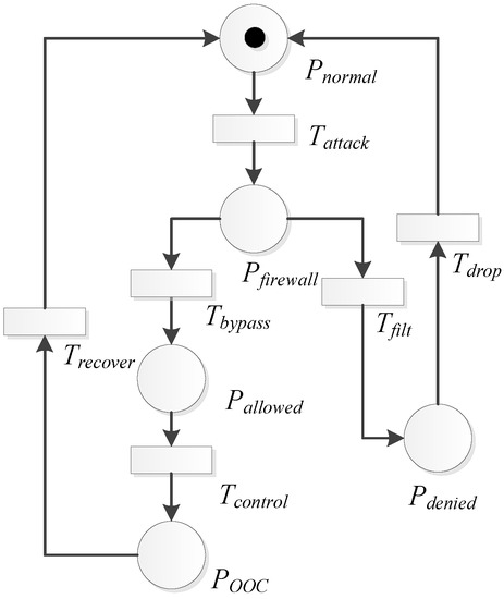
Figure 7. Defense Scenario I: the SPN model.

Table 2. Reachable markings’ set of Scenario I.

	${\mathit{P}}_{\mathit{normal}}$	${\mathit{P}}_{\mathit{firewall}}$	${\mathit{P}}_{\mathit{allowed}}$	${\mathit{P}}_{\mathit{denied}}$	${\mathit{P}}_{\mathit{OOC}}$
$M_0$	1	0	0	0	0
$M_1$	0	1	0	0	0
$M_2$	0	0	1	0	0
$M_3$	0	0	0	0	1
$M_4$	0	0	0	1	0

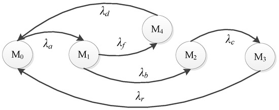
Figure 8. Defense Scenario I: the isomorphic model with the MC and the process of SPN.

As shown in Figure 7, the places $P_{normal}$, $P_{firewall}$, $P_{allowed}$, $P_{denied}$ and $P_{OOC}$ represent the system states, and the transitions $T_{attack}$, $T_{filt}$, $T_{drop}$, $T_{bypass}$ and $T_{control}$ represent the events that enable the transfer of the system state. Initially, the system is in normal state $P_{normal}$. When the transition $T_{attack}$ is triggered, the system transfers to the state $P_{firewall}$. If the firewall finds a matched filter rule from its rules’ database, $T_{filt}$ will be triggered, and the system will transfer into the denied state $P_{denied}$. After that, the $T_{drop}$ transition will be triggered, and the legitimate data will be dropped. Then, the system transfers to the normal state. If the firewall does not find any corresponding filter rule, the transition $T_{bypass}$ will be triggered, and the system will be in state $P_{allowed}$. By triggering the transition $T_{control}$, it will start the attack process, and finally, the system will be out of control, i.e., in state $P_{OOC}$. Then, the administrator recovers the system, and the transition $T_{recover}$ will be triggered. Finally, the system will recover to state $P_{normal}$.

According to the definition of the transition matrix and other performance metrics in [29], we can estimate the SPN model as follows. The transition matrix Q of the SPN model is:

$$Q=\left[\begin{array}{ccccc}-{\lambda }_a& {\lambda }_a& 0& 0& 0\\ 0& -{\lambda }_b-{\lambda }_f& {\lambda }_b& 0& 0\\ 0& 0& -{\lambda }_c& {\lambda }_c& 0\\ {\lambda }_r& 0& 0& -{\lambda }_r& 0\\ {\lambda }_d& 0& 0& 0& -{\lambda }_d\end{array}\right].$$

The steady state probability can be obtained as:

$$\begin{array}{c}{p}_0=({\lambda }_b+{\lambda }_f){{\lambda }_a}^{-1}{p}_1,\hfill \\ p_1=1/\{1+({\lambda }_b+{\lambda }_f)/{\lambda }_a+{\lambda }_b/{\lambda }_c+{\lambda }_b/{\lambda }_r+{\lambda }_f/{\lambda }_d\},\hfill \\ p_2={\lambda }_b/\{{\lambda }_b+{\lambda }_c+{\lambda }_c({\lambda }_b+{\lambda }_f)/{\lambda }_a+{\lambda }_c({\lambda }_b/{\lambda }_r+{\lambda }_f/{\lambda }_d)\},\hfill \\ p_3={\lambda }_b/\{{\lambda }_b+{\lambda }_r+{\lambda }_r[({\lambda }_b+{\lambda }_f)/{\lambda }_a+{\lambda }_b/{\lambda }_c+{\lambda }_f/{\lambda }_d]\},\hfill \\ p_4={\lambda }_f/\{{\lambda }_d+{\lambda }_f+{\lambda }_d[({\lambda }_b+{\lambda }_f)/{\lambda }_a+{\lambda }_b/{\lambda }_r+{\lambda }_b/{\lambda }_c]\}.\hfill \end{array}$$

With the above steady state probability, the token density function can be obtained as:

$$\begin{array}{c}p\left[M(P_{normal}=1)\right]=p\left[M_0\right]=p_0,\hfill \\ p\left[M(P_{firewall}=1)\right]=p\left[M_1\right]=p_1,\hfill \\ p\left[M(P_{allowed}=1)\right]=p\left[M_2\right]=p_2,\hfill \\ p\left[M(P_{denied}=1)\right]=p\left[M_4\right]=p_4,\hfill \\ p\left[M(P_{OOC}=1)\right]=p\left[M_3\right]=p_3.\hfill \end{array}$$

The average number of the tokens in the place $P_{firewall}$ and $P_{denied}$ is as follows:

$$\begin{array}{c}{\overline{\mu }}_{firewall}=p\left[M(P_{firewall}=1)\right]=p_1,\hfill \\ {\overline{\mu }}_{denied}=p\left[M(P_{denied}=1)\right]=p_4.\hfill \end{array}$$

In the subsystem in which the firewall filters out the legitimate data and makes the system transfer to the normal state, the average token number of the place set $\overline{N}$ is the sum of ${\overline{\mu }}_{firewall}$ and ${\overline{\mu }}_{denied}$. That is, $\overline{N}={\overline{\mu }}_{firewall}+{\overline{\mu }}_{denied}$. The utilization rate of the transition $T_{flit}$ is $U(T_{flit})=p_1$. Thus, the token velocity of the transition $R(T_{flit},P_{denied})$ in the subsystem can be obtained as $R(T_{flit},P_{denied})=W(T_{flit},P_{denied})\times U(T_{flit})\times {\lambda }_f=p_1\times {\lambda }_f$, where $W(T_{flit},P_{denied})$ is set as one by default.

Moreover, we can estimate the performance of Defense Scenario I based on the above inferred parameters. The probability of the defense mechanism $P_{defense}$ is the steady probability $p_4$ that the firewall successfully protects the system from attacking, i.e.,

$$P_{defense}=p_4.$$

(9)

The probability $P_{fall}$ that the system falls is the steady probability $p_3$ that the intruder takes control of the system, i.e.,

$$P_{fall}=p_3.$$

(10)

The security probability, denoted as $P_{security}$, is the probability that the system is not exposed to the intruders and does not lose control, i.e.,

$$P_{security}=1-p_2-p_3,$$

(11)

where $p_2$ is the steady probability that the intruder bypasses the firewall and the target system is completely exposed to the intruder.

We also need to analyze the time that the firewall consumes to protect the system. In the subsystem mentioned above, we can get the average token number of the place set $\overline{N}$ and the token velocity of the transition $R(T_{flit},P_{denied})$. According to the little rules and balance principle [30], the delay for the firewall to detect and deal with the aggressive data can be formulated as:

$$T_F=\overline{N}/R(T_{flit},P_{denied})={{\lambda }_f}^{-1}+{{\lambda }_d}^{-1}.$$

(12)

Note that the analysis of the following two SPN models is similar to that of the first SPN model.

4.4. The SPN Model of Scenario II

The SPN model of Defense Scenario II is shown in Figure 9, in which the system is in the detection state of IDS, i.e., $P_{IDS}$, after the firewall is bypassed. If the database of IDS has the matched signature, the transition $T_{detect}$ will be triggered. The system will be in state $P_{matched}$. Then, the system will return to the normal state after the transition $T_{process}$ is enabled. If the IDS cannot identify the intruder, the transition $T_{misdetect}$ is enabled, and the system will be in state $P_{undetected}$. After that, $T_{control}$ will be triggered, and the system state will be transferred as that in Defense Scenario I, shown in Figure 7.

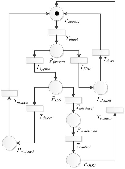
Figure 9. Defense Scenario II: the SPN model.

We denote $\lambda =\{{\lambda }_a,{\lambda }_b,{\lambda }_c,{\lambda }_r,{\lambda }_f,{\lambda }_d,{\lambda }_e,{\lambda }_m,{\lambda }_p\}$ as the average transition triggering rate and $P=\{p_0,p_1,p_2,p_3,p_4,p_5,p_6\}$ as the steady state probability. According to the SPN model in Figure 9, we can obtain the reachable markings’ set $M=\{M_0,M_1,M_2,M_3,M_4,M_5,M_6\}$ and MC as shown in Table 3 and Figure 10.

Table 3. Reachable markings’ set of Scenario II.

	${\mathit{P}}_{\mathit{normal}}$	${\mathit{P}}_{\mathit{firewall}}$	${\mathit{P}}_{\mathit{denied}}$	${\mathit{P}}_{\mathit{IDS}}$	${\mathit{P}}_{\mathit{matched}}$	${\mathit{P}}_{\mathit{undetected}}$	${\mathit{P}}_{\mathit{OOC}}$
$M_0$	1	0	0	0	0	0	0
$M_1$	0	1	0	0	0	0	0
$M_2$	0	0	1	0	0	0	0
$M_3$	0	0	0	1	0	0	0
$M_4$	0	0	0	0	1	0	0
$M_5$	0	0	0	0	0	1	0
$M_6$	0	0	0	0	0	0	1

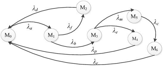
Figure 10. Defense Scenario II: the isomorphic model with the MC and the making process of SPN.

The transition matrix Q is:

$$Q=\left[\begin{array}{ccccccc}-{\lambda }_a& {\lambda }_a& 0& 0& 0& 0& 0\\ 0& -{\lambda }_f-{\lambda }_b& {\lambda }_f& {\lambda }_b& 0& 0& 0\\ {\lambda }_d& 0& -{\lambda }_d& 0& 0& 0& 0\\ 0& 0& 0& -{\lambda }_e-{\lambda }_m& {\lambda }_e& {\lambda }_m& 0\\ {\lambda }_p& 0& 0& 0& -{\lambda }_p& 0& 0\\ 0& 0& 0& 0& 0& -{\lambda }_c& {\lambda }_c\\ {\lambda }_r& 0& 0& 0& 0& 0& -{\lambda }_r\end{array}\right].$$

The state steady probability is:

$$\begin{array}{c}{p}_0=({\lambda }_f+{\lambda }_b){{\lambda }_a}^{-1}{p}_1,\hfill \\ p_1=1/[1+({\lambda }_f+{\lambda }_b){{\lambda }_a}^{-1}+{\lambda }_f{\lambda }_d^{-1}+(1+{\lambda }_e{\lambda }_p^{-1}+{\lambda }_m{\lambda }_c^{-1}+{\lambda }_m{\lambda }_r^{-1}){\lambda }_b/({\lambda }_e+{\lambda }_m)],\hfill \\ p_2={\lambda }_f{\lambda }_d^{-1}{p}_1,\hfill \\ p_3=1/\{{{\lambda }_b}^{-1}({\lambda }_e+{\lambda }_m)[1+({\lambda }_f+{\lambda }_b){{\lambda }_a}^{-1}+{\lambda }_f{\lambda }_d^{-1}]+1+{\lambda }_e{\lambda }_p^{-1}+{\lambda }_m{\lambda }_c^{-1}+{\lambda }_m{\lambda }_r^{-1}\},\hfill \\ p_4={\lambda }_e{\lambda }_p^{-1}{p}_3,\hfill \\ p_5={\lambda }_m{\lambda }_c^{-1}{p}_3,\hfill \\ p_6={\lambda }_m{\lambda }_r^{-1}{p}_3.\hfill \end{array}$$

The token density function is:

$$\begin{array}{ll}p\left[M(P_{normal}=1)\right]=p_0,& p\left[M(P_{firewall}=1)\right]=p_1,\\ p\left[M(P_{denied}=1)\right]=p_2,& p\left[M(P_{IDS}=1)\right]=p_3,\\ p\left[M(P_{matched}=1)\right]=p_4,& p\left[M(P_{undetected}=1)\right]=p_5,\\ p\left[M(P_{OOC}=1)\right]=p_6.& \end{array}$$

The average number of the tokens in a place is:

$$\begin{array}{ccc}{\overline{\mu }}_{normal}=p_0,\hfill & {\overline{\mu }}_{firewall}=p_1,& {\overline{\mu }}_{denied}=p_2,\\ {\overline{\mu }}_{IDS}=p_3,\hfill & {\overline{\mu }}_{matched}=p_4,& {\overline{\mu }}_{undetected}=p_5,\\ {\overline{\mu }}_{OOC}=p_6.\hfill & & \end{array}$$

The utilization rate of the transition is:

$$\begin{array}{ll}U(T_{attack})=p_0,& U(T_{filt})=U(T_{bypass})=p_1,\\ U(T_{drop})=p_2,& U(T_{detect})=U(T_{misdetect})=p_3,\\ U(T_{process})=p_4,& U(T_{control})=p_5,\\ U(T_{re\mathrm{cov}er})=p_6.& \end{array}$$

Then, we can get the token velocity of the transition as:

$$\begin{array}{c}R(T_{filt},P_{denied})=W(T_{filt},P_{denied})\times U\left(T_{filt}\right)\times {\lambda }_f\hfill \\ =p_1\times {\lambda }_f,\hfill \\ R(T_{bypass},P_{IDS})=W(T_{bypass}{P}_{\mathrm{IDS}})\times U\left(T_{bypass}\right)\times {\lambda }_b\hfill \\ =p_1\times {\lambda }_b,\hfill \\ R(T_{detect},P_{matched}=W(T_{detect},P_{matched})\times U\left(T_{detect}\right)\times {\lambda }_e\hfill \\ =p_3\times {\lambda }_e.\hfill \end{array}$$

The probability $P_{defense}$ that the defense mechanism works effectively is the sum of the steady probability $p_2$ and $p_4$, where $p_2$ represents the probability that the firewall detects the attack and $p_2$ represents the probability that the IDS detects the attack. Then, we can get:

$$P_{defense}=p_2+p_4.$$

(13)

The fall probability of the system, denoted as $P_{fall}$, is the steady state probability $p_6$ that the intruder takes control of the system, i.e.,

$$P_{fall}=p_6.$$

(14)

The security probability, denoted as $P_{security}$, that the system is not exposed to the intruder and does not lose control, can be formulated as:

$$P_{security}=1-p_5-p_6.$$

(15)

The subsystem in which the firewall detects and deals with the attack is the same as that mentioned in Scenario I. The average token number of the place set ${\overline{N}}_F$ is the sum of ${\overline{\mu }}_{firewall}$ and ${\overline{\mu }}_{denied}$, i.e., ${\overline{N}}_F={\overline{\mu }}_{firewall}+{\overline{\mu }}_{denied}$. Therefore, the delay $T_F$ introduced by the firewall is:

$$T_F={\overline{N}}_F/R(T_{flit},P_{denied})={{\lambda }_f}^{-1}+{{\lambda }_d}^{-1}.$$

(16)

The delay for the IDS to detect and process the attack behavior can be formulated as:

$$T_D={{\lambda }_b}^{-1}+{{\lambda }_e}^{-1}+{{\lambda }_p}^{-1}.$$

(17)

When the IDS works, it indicates that the intruder has bypassed the firewall without being detected.

4.5. The SPN Model of Scenario III

The SPN model of the Defense Scenario III is shown in Figure 11. We represent the average transition triggering rate as $\lambda =\{{\lambda }_a,{\lambda }_b,{\lambda }_f,{\lambda }_d,{\lambda }_e,{\lambda }_p,{\lambda }_m,{\lambda }_v,{\lambda }_t,{\lambda }_c,{\lambda }_r\}$ and the steady state probability as $P=\{p_0,p_1,p_2,p_3,p_4,p_5,p_6,p_7\}$. According to the model and assumptions, we can get its reachable markings’ set $M=\{M_0,M_1,M_2,M_3,M_4,M_5,M_6,M_7\}$ and MC, as shown in Table 4 and Figure 12.

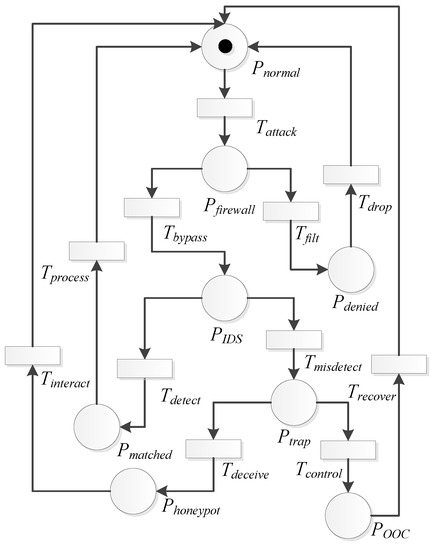
Figure 11. Defense Scenario III: the SPN model.

Table 4. Reachable markings’ set of Scenario III.

	${\mathit{P}}_{\mathit{normal}}$	${\mathit{P}}_{\mathit{firewall}}$	${\mathit{P}}_{\mathit{denied}}$	${\mathit{P}}_{\mathit{IDS}}$	${\mathit{P}}_{\mathit{matched}}$	${\mathit{P}}_{\mathit{trap}}$	${\mathit{P}}_{\mathit{honeypot}}$	${\mathit{P}}_{\mathit{OOC}}$
$M_0$	1	0	0	0	0	0	0	0
$M_1$	0	1	0	0	0	0	0	0
$M_2$	0	0	1	0	0	0	0	0
$M_3$	0	0	0	1	0	0	0	0
$M_4$	0	0	0	0	1	0	0	0
$M_5$	0	0	0	0	0	1	0	0
$M_6$	0	0	0	0	0	0	1	0
$M_7$	0	0	0	0	0	0	0	1

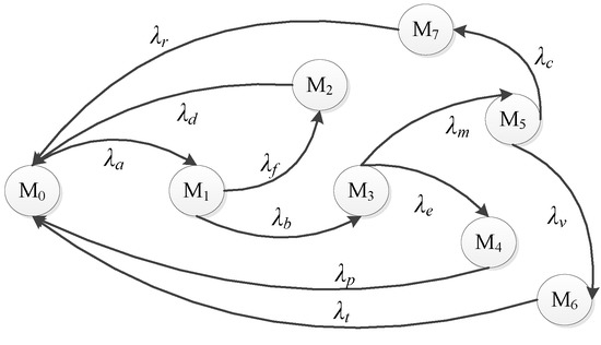
Figure 12. Defense Scenario III: the isomorphic model with the MC and the making process of SPN.

In Figure 11, the honeypot works only after the firewall is bypassed and the IDS cannot identify the legitimate data. The intruder will detect the trap $P_{trap}$ set up by the honeypot. On the one hand, if the intruder cannot identify the trap, it will be in the state $P_{honeypot}$ with the transition $T_{deceive}$ being enabled. The intruder will be deceived to interact with the honeypot. Therefore, the system will recover to the normal state $P_{normal}$ with the the transition $T_{interact}$. On the other hand, if the intruders identify the trap, $T_{control}$ is triggered, and the system state will transfer as described in Figure 7 and Figure 9.

The transition matrix Q is:

$$Q=\left[\begin{array}{cccccccc}-{\lambda }_a& {\lambda }_a& 0& 0& 0& 0& 0& 0\\ 0& -{\lambda }_f-{\lambda }_b& {\lambda }_f& {\lambda }_b& 0& 0& 0& 0\\ {\lambda }_d& 0& -{\lambda }_d& 0& 0& 0& 0& 0\\ 0& 0& 0& -{\lambda }_e-{\lambda }_m& {\lambda }_e& {\lambda }_m& 0& 0\\ {\lambda }_p& 0& 0& 0& -{\lambda }_p& 0& 0& 0\\ 0& 0& 0& 0& 0& -{\lambda }_v-{\lambda }_c& {\lambda }_v& {\lambda }_c\\ {\lambda }_t& 0& 0& 0& 0& 0& -{\lambda }_t& 0\\ {\lambda }_r& 0& 0& 0& 0& 0& 0& -{\lambda }_r\end{array}\right].$$

The state steady probability is:

$$\begin{array}{c}{p}_0=({\lambda }_f+{\lambda }_b){{\lambda }_a}^{-1}{p}_1,\hfill \\ p_1=1/[1+({\lambda }_f+{\lambda }_b){{\lambda }_a}^{-1}+{\lambda }_f{{\lambda }_d}^{-1}+{\lambda }_b{({\lambda }_e+{\lambda }_m)}^{-1}(1+{\lambda }_e{{\lambda }_p}^{-1})\hfill \\ +{\lambda }_b{\lambda }_m{({\lambda }_e+{\lambda }_m)}^{-1}{({\lambda }_v+{\lambda }_c)}^{-1}(1+{\lambda }_v{{\lambda }_t}^{-1}+{\lambda }_c{{\lambda }_r}^{-1})],\hfill \\ p_2={\lambda }_f{\lambda }_d^{-1}{p}_1,\hfill \\ p_3={\lambda }_b{({\lambda }_e+{\lambda }_m)}^{-1}{p}_1,\hfill \\ p_4={\lambda }_e{{\lambda }_p}^{-1}{p}_3,\hfill \\ p_5={\lambda }_m{({\lambda }_v+{\lambda }_c)}^{-1}{p}_3,\hfill \\ p_6={\lambda }_v{{\lambda }_t}^{-1}{p}_5,\hfill \\ p_7={\lambda }_c{{\lambda }_r}^{-1}{p}_5.\hfill \end{array}$$

The token density function is:

$$\begin{array}{ll}p\left[M(P_{normal}=1)\right]=p_0,& p\left[M(P_{firewall}=1)\right]=p_1,\\ p\left[M(P_{denied}=1)\right]=p_2,& p\left[M(P_{IDS}=1)\right]=p_3,\\ p\left[M(P_{matched}=1)\right]=p_4,& p\left[M(P_{trap}=1)\right]=p_5,\\ p\left[M(P_{honeypot}=1)\right]=p_6,& p\left[M(P_{OOC}=1)\right]=p_7.\end{array}$$

The average number of the tokens in a place is:

$$\begin{array}{lll}{\overline{\mu }}_{normal}=p_0,& {\overline{\mu }}_{firewall}=p_1,& {\overline{\mu }}_{denied}=p_2,\\ {\overline{\mu }}_{IDS}=p_3,& {\overline{\mu }}_{matched}=p_4,& {\overline{\mu }}_{trap}=p_5,\\ {\overline{\mu }}_{honeypot}=p_6,& {\overline{\mu }}_{OOC}=p_7.& \end{array}$$

The utilization rate of the transition is:

$$\begin{array}{ll}U(T_{attack})=p_0,& U(T_{filt})=U(T_{bypass})=p_1,\\ U(T_{drop})=p_2,& U(T_{detect})=U(T_{misdetect})=p_3,\\ U(T_{process})=p_4,& U(T_{deceive})=U(T_{control})=p_5,\\ U(T_{\mathrm{int}eract})=p_6,& U(T_{re\mathrm{cov}er})=p_7.\end{array}$$

The token velocity of the transition is:

$$\begin{array}{ll}R(T_{filt},P_{denied})=p_1\times {\lambda }_f,& R(T_{bypass},P_{IDS})=p_1\times {\lambda }_b,\\ R(T_{detect},P_{matched})=p_3\times {\lambda }_e,& R(T_{misdetect},P_{trap})=p_3\times {\lambda }_m,\\ R(T_{deceive},P_{honeypot})=p_5\times {\lambda }_v.& \end{array}$$

Based on the above equations, we can obtain the probability of protecting the system from attacking, denoted as $P_{defense}$, as:

$$P_{defense}=p_2+p_4+p_6,$$

(18)

where $p_2$, $p_4$ and $p_6$ represent the steady state probabilities that each of the firewall, IDS and honeypot prevents the intrusion behaviors, respectively.

The system fall probability $P_{fall}$ is the steady state probability $p_7$ that the system is completely controlled by the intruder, i.e.,

$$P_{fall}=p_7.$$

(19)

The security probability $P_{security}$ can be formulated as:

$$P_{security}=1-p_5-p_7,$$

(20)

where $p_5$ is the steady probability that the intruder can identify the trap set up by the honeypot.

The time delays that each of the firewall, IDS and honeypot consume respectively in Defense Scenario III can be formulated as:

$$\begin{array}{c}{T}_F={{\lambda }_f}^{-1}+{{\lambda }_d}^{-1},\hfill \\ T_D={{\lambda }_b}^{-1}+{{\lambda }_e}^{-1}+{{\lambda }_p}^{-1},\hfill \\ T_H={{\lambda }_b}^{-1}+{{\lambda }_m}^{-1}+{{\lambda }_v}^{-1}+{{\lambda }_t}^{-1}.\hfill \end{array}$$

(21)

5. Performance Evaluation

In this section, we implement the proposed three SPN models on the PIPE platform. To compare and evaluate the performance of the honeypot, we set the parameters as shown in Table 5. $Par.$ represents the average transition triggering rate, and $Val.$ is the corresponding value of the rate. Note that, $det\_rate$, $dec\_rate$ and $int\_rate$ correspond to ${\lambda }_e$, ${\lambda }_v$ and ${\lambda }_t$, respectively. We can get the three scenarios’ transition triggering rates from Table 5. We set the parameters with the SPN models to conduct further simulations on the PIPE platform. We first present the simulation results. Then, we conduct the performance comparison among the proposed three SPN models.

Table 5. Parameters of the SPN models.

$\mathit{Par}.$	$\mathit{Val}.$	$\mathit{Par}.$	$\mathit{Val}.$	$\mathit{Par}.$	$\mathit{Val}.$	$\mathit{Par}.$	$\mathit{Val}.$
$att\_rate$	4	$drop\_rate$	3	$mis\_rate$	1	$ctrl\_rate$	2
$byp\_rate$	2	$det\_rate$	1	$dec\_rate$	2	$rec\_rate$	4
$filt\_rate$	2	$pro\_rate$	3	$int\_rate$	0.5

5.1. Simulation Results

The transition triggering rate of the Defense Scenario I’s SPN model shown in Table 6 can be obtained from Table 5. With the simulation, we can get the reachable markings’ set as shown in Table 7 and the reachable graph in Figure 13. We can see that Table 7 is actually the same as Table 2 in Section 4.3, although the identifiers are not consistent. According to MC’s acquiring process of replacing the reachable graph’s transitions with transition triggering rates [29], we can find that the MC in Section 4.3 is correct. Furthermore, we can get the steady state probability in the simulation as illustrated in Table 8.

Table 6. The average transition triggering rate of Scenarios I/II/III.

	${\mathit{\lambda }}_{\mathit{a}}$	${\mathit{\lambda }}_{\mathit{b}}$	${\mathit{\lambda }}_{\mathit{f}}$	${\mathit{\lambda }}_{\mathit{d}}$	${\mathit{\lambda }}_{\mathit{c}}$	${\mathit{\lambda }}_{\mathit{r}}$	${\mathit{\lambda }}_{\mathit{e}}$	${\mathit{\lambda }}_{\mathit{p}}$	${\mathit{\lambda }}_{\mathit{m}}$	${\mathit{\lambda }}_{\mathit{v}}$	${\mathit{\lambda }}_{\mathit{t}}$
Scenario I	4	2	2	3	2	4	-	-	-	-	-
Scenario II	4	2	2	3	2	4	1	3	1	-	-
Scenario III	4	2	2	3	2	4	1	3	1	2	0.5

Table 7. Reachable markings’ set of Scenario I.

	${\mathit{P}}_{\mathit{normal}}$	${\mathit{P}}_{\mathit{firewall}}$	${\mathit{P}}_{\mathit{allowed}}$	${\mathit{P}}_{\mathit{denied}}$	${\mathit{P}}_{\mathit{OOC}}$
$M_0$	1	0	0	0	0
$M_1$	0	1	0	0	0
$M_2$	0	0	0	1	0
$M_3$	0	0	1	0	0
$M_4$	0	0	0	0	1

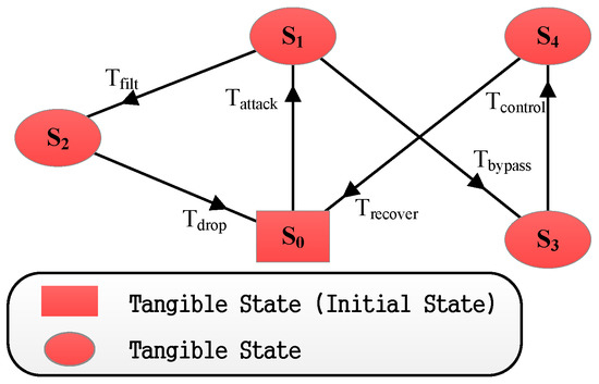
Figure 13. The reachable graph for Scenario I.

Table 8. The steady state probability of Scenarios I/II/III.

$\mathit{Pro}.$	Scenario I	Scenario II	Scenario III
$p_0$	0.24	0.21053	0.18605
$p_1$	0.24	0.21053	0.18605
$p_2$	0.24	0.14035	0.12403
$p_3$	0.12	0.21053	0.18605
$p_4$	0.16	0.10526	0.04651
$p_5$	—	0.07018	0.06202
$p_6$	—	0.05263	0.18605
$p_7$	—	—	0.02326

Firstly, we obtain the transition triggering rate (shown in Table 6) from Table 5. Then, we conduct the simulations, the results of which are illustrated in Table 9, Table 8 and Figure 14.

Table 9. Reachable markings’ set of Scenario II.

	${\mathit{P}}_{\mathit{normal}}$	${\mathit{P}}_{\mathit{firewall}}$	${\mathit{P}}_{\mathit{denied}}$	${\mathit{P}}_{\mathit{IDS}}$	${\mathit{P}}_{\mathit{matched}}$	${\mathit{P}}_{\mathit{undetected}}$	${\mathit{P}}_{\mathit{OOC}}$
$M_0$	1	0	0	0	0	0	0
$M_1$	0	1	0	0	0	0	0
$M_2$	0	0	1	0	0	0	0
$M_3$	0	0	0	1	0	0	0
$M_4$	0	0	0	0	0	1	0
$M_5$	0	0	0	0	1	0	0
$M_6$	0	0	0	0	0	0	1

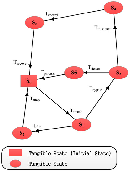
Figure 14. The reachable graph for Scenario II.

Similarly, we get the transition triggering rate (shown in Table 6) from Table 5 firstly. We get the results of the reachable markings’ set and reachable graph (illustrated in Table 10 and Figure 15) to validate the theoretical analysis. We obtain the steady state probability for further performance evaluation as illustrated in Table 8.

Table 10. Reachable markings’ set of Scenario III.

	${\mathit{P}}_{\mathit{normal}}$	${\mathit{P}}_{\mathit{firewall}}$	${\mathit{P}}_{\mathit{denied}}$	${\mathit{P}}_{\mathit{IDS}}$	${\mathit{P}}_{\mathit{matched}}$	${\mathit{P}}_{\mathit{trap}}$	${\mathit{P}}_{\mathit{honeypot}}$	${\mathit{P}}_{\mathit{OOC}}$
$M_0$	1	0	0	0	0	0	0	0
$M_1$	0	1	0	0	0	0	0	0
$M_2$	0	0	1	0	0	0	0	0
$M_3$	0	0	0	1	0	0	0	0
$M_4$	0	0	0	0	0	1	0	0
$M_5$	0	0	0	0	1	0	0	0
$M_6$	0	0	0	0	0	0	1	0
$M_7$	0	0	0	0	0	0	0	1

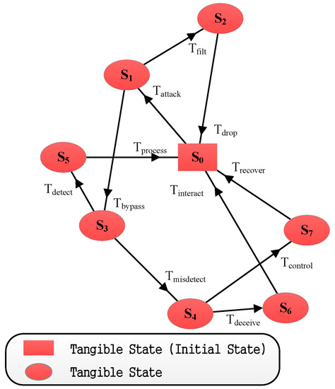
Figure 15. The reachable graph for Scenario III.

5.2. Performance Comparison

With the data we get from the above simulations and the equations of the three scenarios in Section 4, we can figure out the fall probability $P_{fall}$, the security probability $P_{security}$, the defense probability $P_{defense}$ and the delays, as shown in Table 11.

Table 11. Analysis results of probability and delay.

	Scenario I	Scenario II	Scenario III
$P_{defense}$	0.16	0.21053	0.3721
$P_{fall}$	0.12	0.05263	0.02326
$P_{security}$	0.64	0.84211	0.93023
$T_F$	0.8333	0.8333	0.8333
$T_D$	—-	1.8333	1.8333
$T_H$	—-	—-	4.0

By analyzing the data in Table 11, we can see that with the IDS and honeypot added into the defense mechanism one by one, the security probability of the system and the defense level are both increasing gradually. In contrast, the probability of the system being taken over declines and drops to 2.326%.

Table 11 also shows the delay of the defense techniques in different scenarios. It illustrates that the firewall delay is the same in the three scenarios and the IDS delay is the same in Scenario II and Scenario III. The honeypot delay is the highest one compared with that of the firewall and IDS. The system’s total delay increases sharply in Scenario III.

In summary, the honeypot can enforce the defense level of the computer system at the expense of much more time consumption. Hence, it is suggested that the administrator determine whether to deploy the honeypot or not in the defense mechanism according to the environment and the clients’ requirements on security to avoid wasting the system resource.

6. Conclusions

In this paper, we focus on the performance analysis of the honeypot. Firstly, we proposed three system defense scenarios and constructed performance evaluation models based on stochastic Petri nets. Then, we theoretically analyzed the proposed three SPN models. After that, we conducted the extensive simulations on the PIPE platform, the results of which illustrate the effectiveness in security enhancement of the honeypot under the proposed SPN models.

This paper provides a new way to evaluate the performance of the honeypot system. In some information fields with higher requirements of confidentiality, such as the army combat command system, government office network, large enterprise servers, etc., we can decide whether to choose a honeypot to strengthen the defense and protection of the system according to the actual needs and then estimate the system safety probability, defense success probability, etc. The work can guide the honeypot deployment and improve the comprehensive protective performance of the system.

References

- Cheminod, M.; Durante, L.; Seno, L.; Valenzano, A. Performance evaluation and modeling of an industrial application-layer firewall. IEEE Trans. Ind. Inform. 2018, 5, 2159–2170. [Google Scholar] [CrossRef]
- Jiang, C.B.; Liu, I.H.; Chung, Y.N.; Li, J.S. Novel intrusion prediction mechanism based on honeypot log similarity. Int. J. Netw. Manag. 2016, 3, 156–175. [Google Scholar] [CrossRef]
- Paradise, A.; Shabtai, A.; Puzis, R.; Elyashar, A.; Elovici, Y.; Roshandel, M.; Peylo, C. Creation and Management of Social Network Honeypots for Detecting Targeted Cyber Attacks. IEEE Trans. Comput. Soc. Syst. 2017, 3, 65–79. [Google Scholar] [CrossRef]
- Wang, K.; Du, M.; Maharjan, S.; Sun, Y. Strategic honeypot game model for distributed denial of service attacks in the smart grid. IEEE Trans. Smart Grid 2017, 5, 2474–2482. [Google Scholar] [CrossRef]
- Maione, G.; Mangini, A.M.; Ottomanelli, M. A generalized stochastic petri net approach for modeling activities of human operators in intermodal container terminals. IEEE Trans. Autom. Sci. Eng. 2016, 4, 1504–1516. [Google Scholar] [CrossRef]
- List, G.F.; Mashayekhi, M. A modular colored stochastic Petri net for modeling and analysis of signalized intersections. IEEE Trans. Intell. Trans. Syst. 2016, 3, 701–713. [Google Scholar] [CrossRef]
- Dhaliwal, S.S.; Nahid, A.; Abbas, R. Effective intrusion detection system using XGBoost. Information 2018, 9, 149. [Google Scholar] [CrossRef]
- Liu, M.; Zhang, Q.; Zhao, H.; Yu, D. Network security situation assessment based on data fusion. In Proceedings of the Advances in Knowledge Discovery and Data Mining, Osaka, Japan, 20–23 May 2008; pp. 542–545. [Google Scholar]
- Romain, L.; Francois, B.; Abdelmalek, B.; Maroun, C. A specification method for analyzing fine grained network security mechanism configurations. In Proceedings of the Communications and Network Security, Washington, DC, USA, 14–16 October 2013; pp. 483–487. [Google Scholar]
- Yuan, H.Q.; Li, Z.H. ARP spoofing and its petri net model. Softw. Guide 2005, 13, 14–16. (In Chinese) [Google Scholar]
- Hwang, H.U.; Kim, M.S.; Noh, B.N. Expert system using fuzzy petri nets in computer forensics. In Proceedings of the First International Conference, ICHIT 2006, Jeju Island, Korea, 9–11 November 2006; pp. 312–322. [Google Scholar]
- Aliannezhadi, Z.; Azgomi, M.A. Modeling and analysis of a web service firewall using coloured petri nets. In Proceedings of the 3rd IEEE Asia-Pacific Services Computing Conference, APSCC 2008, Yilan, Taiwan, 9–12 December 2008; pp. 548–553. [Google Scholar]
- Dolgikh, A.; Nykodym, T.; Skormin, V.; Antonakos, J.; Baimukhamedov, M. Colored Petri nets as the enabling technology in intrusion detection systems. In Proceedings of the 2011 Military Communications Conference, Baltimore, MA, USA, 7–10 November 2011; pp. 1297–1301. [Google Scholar]
- Voron, J.B.; Démoulins, C.; Kordon, F. Adaptable intrusion detection systems dedicated to concurrent programs: A petri net-based approach. In Proceedings of the Tenth International Conference Application of Concurrency to System Design, Braga, Portugal, 21–25 June 2010; pp. 57–66. [Google Scholar]
- Balaz, A.; Vokorokos, L. Intrusion detection system based on partially ordered events and patterns. In Proceedings of the IEEE 13th International Conference on Intelligent Engineering Systems, Barbados, 16–18 April 2009; pp. 233–238. [Google Scholar]
- Toktabayev, A.; Skormin, V.; Dolgikh, A. Obfuscation resilient behavior based ids based on colored petri nets. In Proceedings of the 15th European conference on Research in computer security, Athens, Greece, 20–22 September 2010. [Google Scholar]
- Nykodym, T.; Skormin, V.; Dolgikh, A.; Antonakos, J. Automatic functionality detection in behavior-based ids. In Proceedings of the 2011 Military Communications Conference, Baltimore, MA, USA, 7–10 November 2011; pp. 1302–1307. [Google Scholar]
- Ding, W.B. Security analysis of Intrusion Tolerance System based on Petri Nets. Master’s Thesis, Harbin Institute of Technology, Harbin, China, 2006. [Google Scholar]
- Wang, C.; Ma, J.F. Availability analysis and comparison of different intrusion-tolerant systems. In Content Computing; Spring: Berlin/Heidelberg, Germany, 2004; pp. 161–166. [Google Scholar]
- Yang, J.; Chen, X.; Xiang, X.; Wan, J. HIDS-DT: An effective hybrid intrusion detection system based on decision tree. In Proceedings of the International Conference on Communications and Mobile Computing, Shenzhen, China, 12–14 April 2010; pp. 70–75. [Google Scholar]
- Shi, L.Y.; Jia, C.F.; Lv, S.W. Performance evaluation for service hopping system using stochastic petri net. Acta Scientiarum Naturalium Universitatis Nankaiensis 2009, 1, 72–75. [Google Scholar]
- Teo, L.; Sun, Y.A.; Ahn, G.J. Defeating internet attacks using risk awareness and active honeypots. In Proceedings of the Fifth Annual IEEE SMC Information Assurance Workshop, West Point, NY, USA, 10–11 June 2004; pp. 155–167. [Google Scholar]
- Ding, Z.; Zhou, Y.; Zhou, M. Modeling self-adaptive software systems by fuzzy rules and petri nets. IEEE Trans. Fuzzy Syst. 2018, 26, 967–984. [Google Scholar] [CrossRef]
- Behinaein, B.; Rudie, K.; Sangrar, W. Petri net siphon analysis and graph theoretic measures for identifying combination therapies in cancer. IEEE/ACM Trans. Comput. Biol. Bioinform. 2018, 15, 231–243. [Google Scholar] [CrossRef] [PubMed]
- Wiśniewski, R.; Karatkevich, A.; Adamski, M.; Costa, A.; Gomes, L. Prototyping of concurrent control systems with application of petri nets and comparability graphs. IEEE Trans. Control Syst. Technol. 2018, 26, 575–586. [Google Scholar] [CrossRef]
- Liu, H.C.; Luan, X.; Li, Z.; Wu, J. Linguistic petri nets based on cloud model theory for knowledge representation and reasoning. IEEE Trans. Knowl. Data Eng. 2018, 4, 717–728. [Google Scholar] [CrossRef]
- Gouda, M.G.; Liu, A.X. Structured firewall design. Comput. Netw. 2007, 4, 1106–1120. [Google Scholar] [CrossRef]
- Diaz-Gomez, P.A.; Hougen, D.F. Improved off-line intrusion detection using a Genetic Algorithm. In Proceedings of the 7th International Conference on Enterprise Information Systems, Miami, FL, USA, 25–28 May 2005; pp. 66–73. [Google Scholar]
- Lin, C. Stochastic Petri Net and System Performance Evaluation; Tingshua University: Beijing, China, 2005. [Google Scholar]
- Trivedi, K.S. Probability Statistics with Reliability, Queuing and Computer Science Applications; John Wiley and Son: Hoboken, NJ, USA, 2016. [Google Scholar]
© 2018 by the authors. Licensee MDPI, Basel, Switzerland. This article is an open access article distributed under the terms and conditions of the Creative Commons Attribution (CC BY) license (http://creativecommons.org/licenses/by/4.0/).