Inspired from Ants Colony: Smart Routing Algorithm of Wireless Sensor Network

Abstract

In brief, Wireless Sensor Networks (WSNs) are a set of limited power nodes, used for gathering the determined data of an area. Increasing the lifetime is the main challenge to optimize WSNs routing protocols, since the sensors’ energy in most cases is limited. In this respect, this article introduces a novel smart routing algorithm of wireless sensor networks, consisting of stable nodes randomly dispersed, and this approach is inspired from ant colonies. The proposed algorithm takes into consideration the distance between two nodes, the chosen path length and the nodes’ residual energy so as to update the choice probability of the next node among the neighbouring nodes, contrary to several routing algorithms; on the one hand, the nodes are aggregating data of their predecessors and sending to all to their successors; on the other hand, the source is almost always changed in each iteration. Consequently, the energy consumption is balanced between the nodes. Hence, the network lifetime will be increased. Detailed descriptions and a set of simulation using Matlab is provided to measure the network lifetime and the energy consumed by nodes of the proposed approach are presented. The replications’ consequences of simulations prove the success of our future routing algorithm (SRA).

1. Introduction

In recent years, smaller electronics devices have appeared, so much so that the different wireless networks have emerged. The improvement of data rates and the reduction of energy consumption are the challenges to improve these networks. Higher data rates are required as internet access becomes more popular. That is why, the allocation of more bandwidth, or the processing of advanced signals with spectral efficiency are required. As a matter of fact, the major problem in wireless networks was still the energy consumption [1]. Some emerging wireless network applications are designed to require low data rates. Therefore, the energy consumption concern is greater than that of the high data rates. The wireless sensor network is another type of emerging wireless network where low power consumption is more critical than high data rates. Actually, wireless sensor networks have become a growing field of research and application, with the advancement of information technology [2,3,4,5,6,7]. A sensor array is composed of numbers of sensor nodes scattered randomly in certain regions. These sensor nodes have detection, communication, calculation and power functions [8,9,10,11]. WSNs have been applied in many different applications such as vehicle tracking system, traffic monitoring, medical applications, etc. With built-in detection parts in the nodes, a WSN can monitor and collect information or data in the deployed area. Collected data packets deliver source nodes to the single receiving node, which will cost energy. WSNs give prominence to more simple deployment and good flexibility of devices. With the fast technological development of sensors, which will greatly improve the efficiency and reliability of infrastructure systems, WSNs will evolve into the key technology for Internet of Things (IoT). Among the main concerns related to applications of IoT is extending the battery life of Machine to Machine (M2M) mobile devices to make the IoT system work for a longer period. As a result, in the vast mass of applications of the Internet of Things, energy-efficient communication and stable energy supply have become the priority objectives in the allocation of resources [12]. Several protocols have been implemented—for example, the cluster-based LEACH (Low Energy Adaptive Clustering Hierarchy) [8], which is based on cluster and Directed Diffusion (DD). ACO (Ant Colony Optimization) is a widespread meta-heuristic approach to solving combinatorial optimization problems such as the asymmetric travelling salesman problem, vehicle routing, WSN routing, etc. This algorithm is inspired by the behaviour of ant colonies. Due to the limited power supply, maximizing the lifetime of a WSN is crucial for the performance of the routing protocol. In this article, ACO is adopted and improved to design an intelligent routing algorithm to maximize the lifetime of a WSN. The remainder of the paper is planned as follows. Firstly, Section 2 presents the ant colony optimization algorithm: the ant system and the ant colony system. Secondly, Section 3 describes the algorithm proposed. Thirdly, the results of the simulation are offered and discussed in Section 4. Finally, Section 5 concludes the paper.

2. Ant Colony Optimization Algorithm

Ant colony optimization [13] works in an iterative way. A number of ants are used at each iteration. AS or ant system is the first algorithm in the ACO algorithm category. In the last few decades, there has been a lot of research that uses the ant colony such as: elitist strategy for ant system (EAS), AS_rank, Max-Min AS, or ant colony system (ACS) [14]. In AS, after ants have made their tours, in the process of looking for food, each ant puts out pheromones to form pheromone tracks. After the ants deposit the pheromones, the pheromone parts evaporate over time. Hence, the shorter crossed route by an ant, will have more amount of deposited pheromone. Generally, each ant chooses with more probability the road with more pheromone. So, the long paths receive less pheromones than the short path. The ACS improves AS by making the introduction of a local update of pheromones in the process of building the tour. All the ants perform the update of local pheromone after each construction step. At the end of each iteration, only one ant applies the update of the off-line pheromone, which can be either the best iteration, or the best one so far. The resolution regulation used by the ants throughout the creation procedure is an added essential divergence among ACS and AS. As a matter of fact, ACS use the rule of pseudo random proportional. In our article we will add the residual energy parameter. Hence, an arc belonging to a short path and having more residual energy for these two edges will be more likely to be chosen than the other edges even if they are too short because they have less residual energy.

3. Proposed Algorithm

This part describes our Smart Routing Algorithm (SRA): that all the nodes communicate with each other, if the first node detects an event it will look for its successor, it broadcasts the request message. If a neighbour node receives that request message, it will store the ID of the sender in its list-neighbour firstly and then broadcast its own power and receiver ID and its positioning (x,y) as a response, and then wait for an acknowledgement, if the acknowledgement is received. Hence, these nodes, sender and receiver, are connected and can communicate between them. When all the recipients finish doing the same thing, the node that will send data has its neighbours list, it calculates the probability, $p_{i,j}$, for each candidate j belongs to the list of neighbouring nodes, and then executes line 7 to line 14 of Algorithm 1 for choosing its next best node and sends data to it. After that, the next node receives data, aggregates it with its own and sends all data , using the SRA (Smart Routing Algorithm), to its successor, and this process is repeated until the data arrives at the base station. The first iteration is counted when the data arrives at the base station. This mechanism is repeated until some number of iterations; in our case, we stop at 50 iterations (the nodes are all alive).

The probability that node i sends to node j is given by Equation (1):

$$p_{i,j}=\frac{{\left({\tau }_{i,j}\right)}^{\alpha }·{\left({\eta }_{i,j}\right)}^{\beta }·{\left(E_{res}\left(i\right)\right)}^{\gamma }·{\left(E_{res}\left(j\right)\right)}^{\delta }}{\sum {\left({\tau }_{i,j}\right)}^{\alpha }·{\left({\eta }_{i,j}\right)}^{\beta }·{\left(E_{res}\left(i\right)\right)}^{\gamma }·{\left(E_{res}\left(j\right)\right)}^{\delta }},$$

(1)

where:

• ${\tau }_{i,j}$ is the pheromone amount on edge $(i,j)$,
• ${\eta }_{i,j}$ is is the opportunity of the edge $(i,j)$,
• $\alpha$ is a variable to adjust the effect of ${\tau }_{i,j}$,
• $\beta$ is a variable to adjust the effect of ${\eta }_{i,j}$,
• $E_{res}\left(i\right)$ is the residual energy of node i,
• $E_{res}\left(j\right)$ is the residual energy of node j,
• $\gamma$ is a variable to adjust the effect of $E_{res}\left(i\right)$,
• $\delta$ is a variable to adjust the effect of $E_{res}\left(j\right)$.

The pheromone quantity is renewed and applied to the retraced arcs (backtracking) as shown in the Equation (2):

$${\tau }_{i,j}=(1-\varrho ){\tau }_{i,j}+\Delta {\tau }_{i,j},$$

(2)

where:

• $\varrho$ is the evaporation rate of pheromones,
• $\Delta {\tau }_{(i,j)}$ is the amount of pheromone put, generally offered by:

  $$\Delta {\tau }_{(i,j)}=\left\{\begin{array}{cc}{\displaystyle \frac{1}{L}},\hfill & \mathrm{if} \mathrm{node} i \mathrm{sends} \mathrm{data} \mathrm{to} \mathrm{node} j,\hfill \\ 0,\hfill & \mathrm{otherwise},\hfill \end{array}\right.$$

  (3)

where:

• L is the length of the path,
  The opportunity of the edge $(i,j)$ is given by this equation

  $${\eta }_{(i,j)}=\frac{1}{{\delta }_{(i,j)}}.$$

  (4)

In this work, the WSN nodes send collaboratively their captured data to the sink. We employ the dissipation energy model [15,16] = as shown in Figure 1. In this figure, $E_{T\left(x\right)}(k,\delta )$ is the energy expended for the transmission of k bits along a distance $\delta$, and $E_{Rx}$ is the energy expended to receive a k-bit of data. The element $E_{elec}$ depends on modulation, filtering, digital coding, and the spreading of the signal [16]. This element is the energy dissipated per bit to work both the receiver and the transmitter circuits.

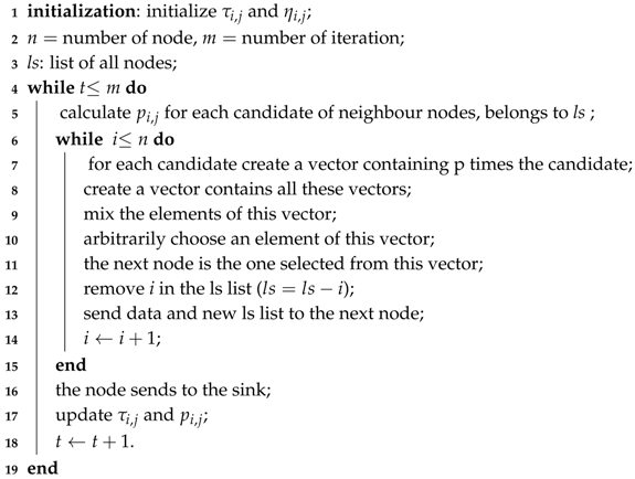
Algorithm 1: Smart Routing Algorithm (SRA)

The energy expended by the radio sender is offered in Equation (5) and by the receiver in Equation (6). Equation (7) is the power needed to aggregate data:

$$E_{t\left(x\right)}(k,\delta )=\left\{\begin{array}{cc}k.E_{elec}+k.E_{fs}.{\delta }^2\hfill & \mathrm{if} \delta <{\delta }_0,\hfill \\ k.E_{elec}+k.E_{mp}.{\delta }^4\hfill & \mathrm{if} \delta \ge {\delta }_0,\hfill \end{array}\right.$$

(5)

$$E_{Rx}=k.E_{elec},$$

(6)

$$E_{agr}=k.E_{DA},$$

(7)

where:

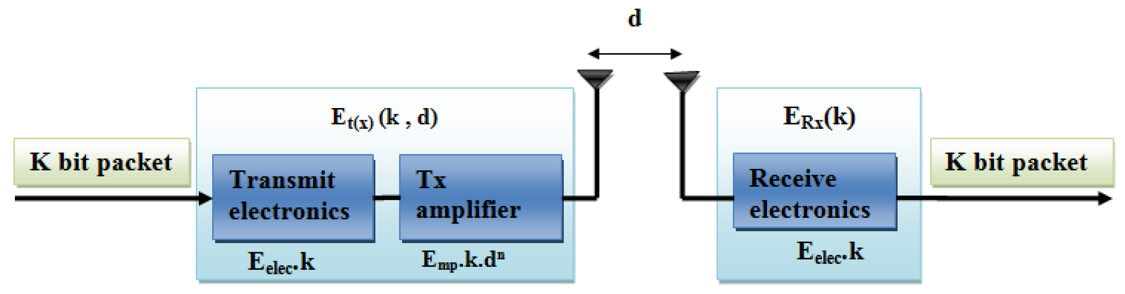
• $\delta$ is the distance among the sender and the addressee,
• $E_{fs}$ and $E_{mp}$ are the amplifier energy, for the first, in the free space model, and, for the second, in the multipath model.

If $\delta$ is below a threshold ${\delta }_0$, then the parameters ${\delta }^2$ and $E_{fs}$ are used; otherwise, the elements ${\delta }^4$ and $E_{mp}$ are employed. The value of the threshold ${\delta }_0$ is shown in [17], and presented in Equation (8):

$${\delta }_0=\sqrt{\frac{E_{fs}}{E_{mp}}}.$$

(8)

In this paper, the first sensor that will send its data takes the value 1, the second takes the value 2, and so on until reaching the base station. These numbers given by the path will be followed along each iteration, using SRA: 1 is the first node that will transmit its data, the number 2 will receive the data of 1, aggregate with its own data and will then send all to node 3. The sensors will receive the data of their predecessors, aggregate with their own data and then send the whole to their successors. This is will repeat until the base station. The routing follows a path that will be chosen using SRA as dynamically. Using Equations (5)–(8), it is possible to adjust for each sensor, 1 to 25, its consumed energy during iterations in Equation (9).

$$E_{iter}\left(i\right)=\left\{\begin{array}{cc}k.(i-1).(E_{elec}+E_{DA})+k.i.(E_{elec}+E_{fs}.{\delta }^2)\hfill & \mathrm{if} \delta <{\delta }_0,\hfill \\ k.(i-1).(E_{elec}+E_{DA})+k.i.(E_{elec}+E_{mp}.{\delta }^4)\hfill & \mathrm{if} \delta \ge {\delta }_0,\hfill \end{array}\right.$$

(9)

where:

• i is the sensor number.

The average energy consumed in a network at each iteration, Equation (10), is the sum of energy consumed by each sensor up to this iteration divided by the number of sensors participating in this network:

$$E_{av{g}_{iter}}=1/n·\sum _{i=1}^n{E}_{iter}\left(i\right),$$

(10)

where:

• n is the number of participating sensors in this network.

The total consumed energy by a sensor, Equation (11), is the energy consumed until the last iteration:

$$E_{tota{l}_{iter}}\left(i\right)=\sum _{iter=1}^{it}{E}_{iter}\left(i\right).$$

(11)

The average consumed energy of network, Equation (12), is the total energy consumed by all sensors divided by sensor number:

$$E_{avg}=1/n·\sum _{i=1}^n{E}_{tota{l}_{iter}}\left(i\right).$$

(12)

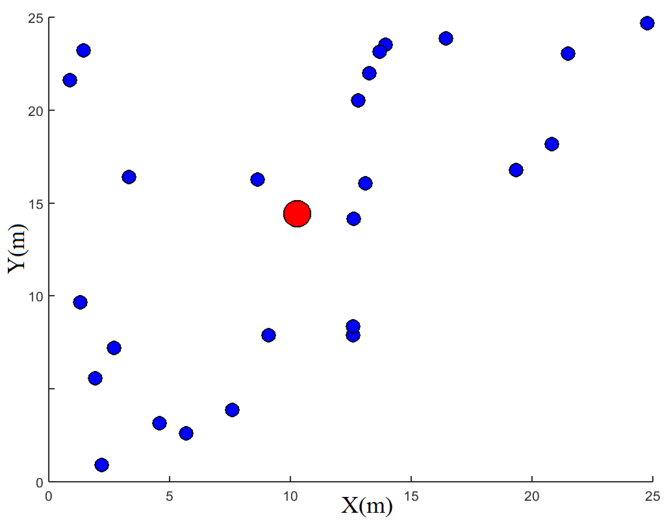
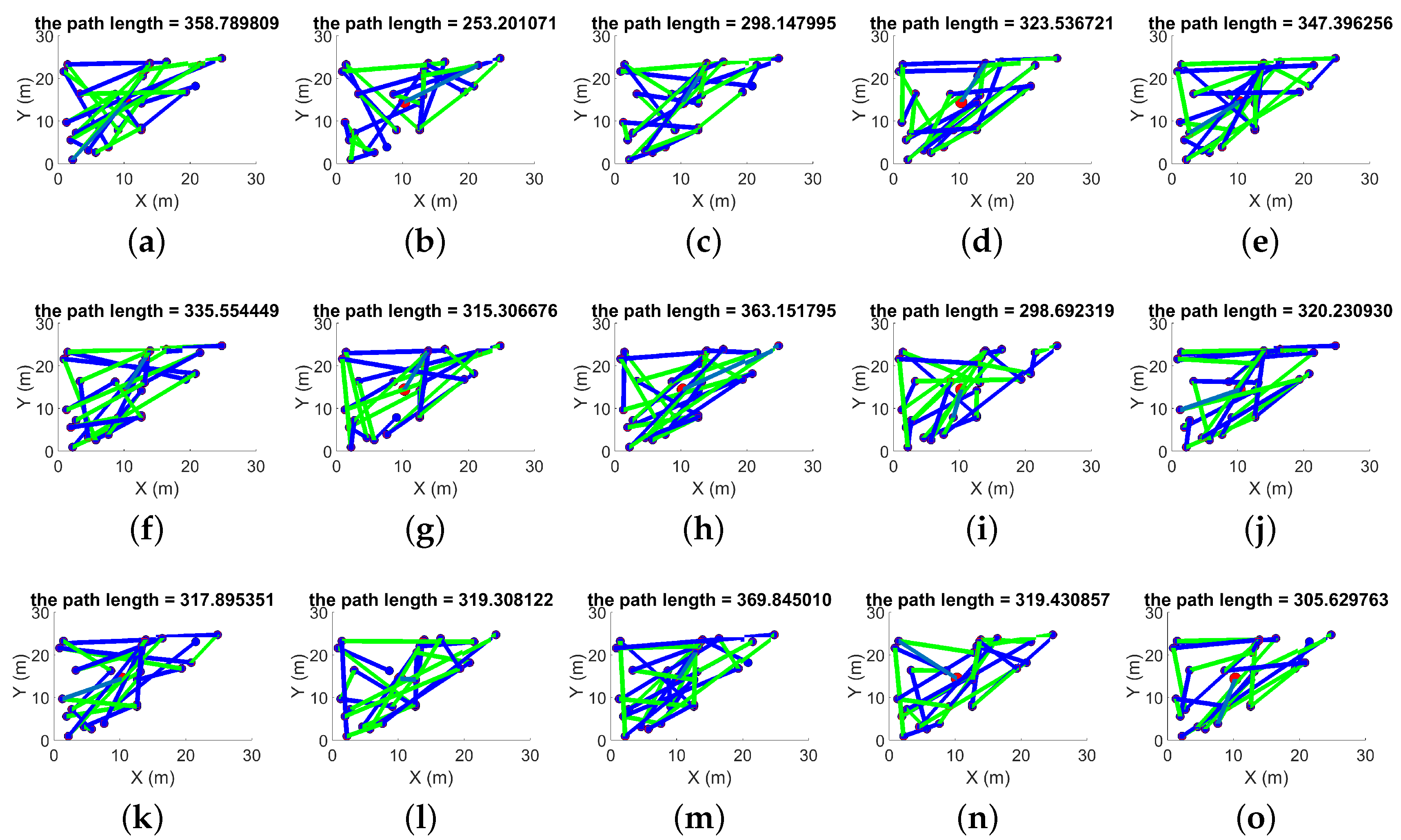
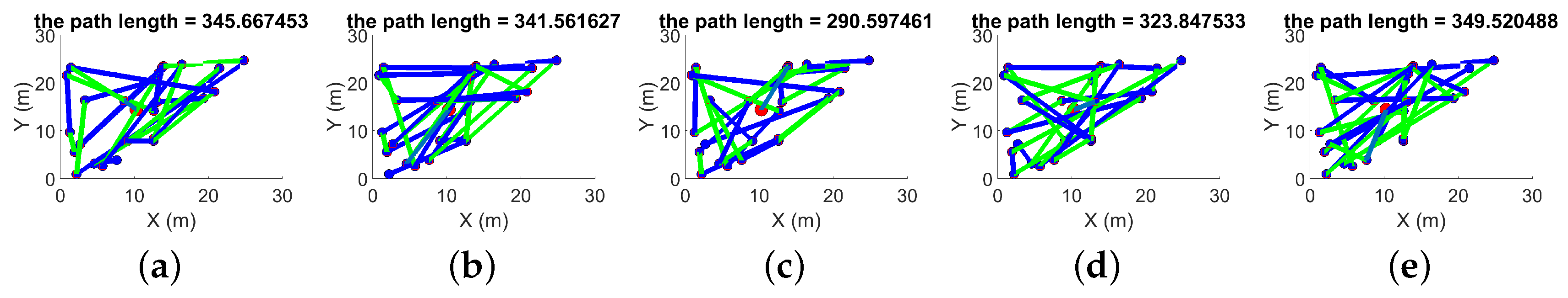
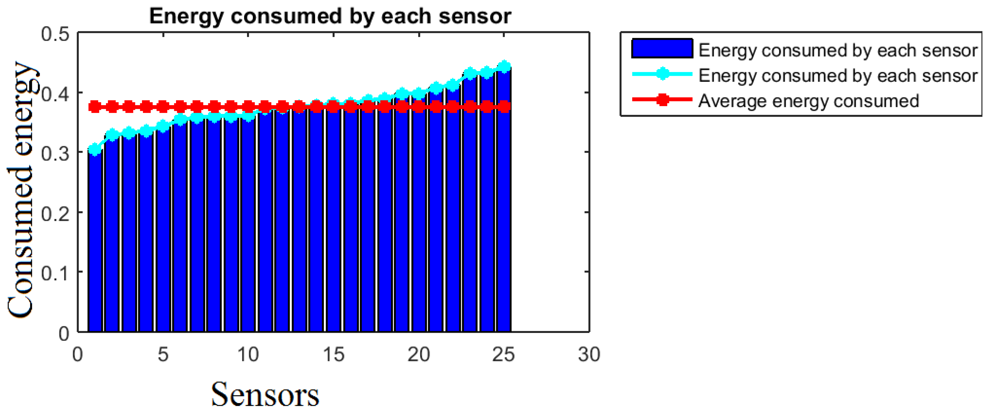
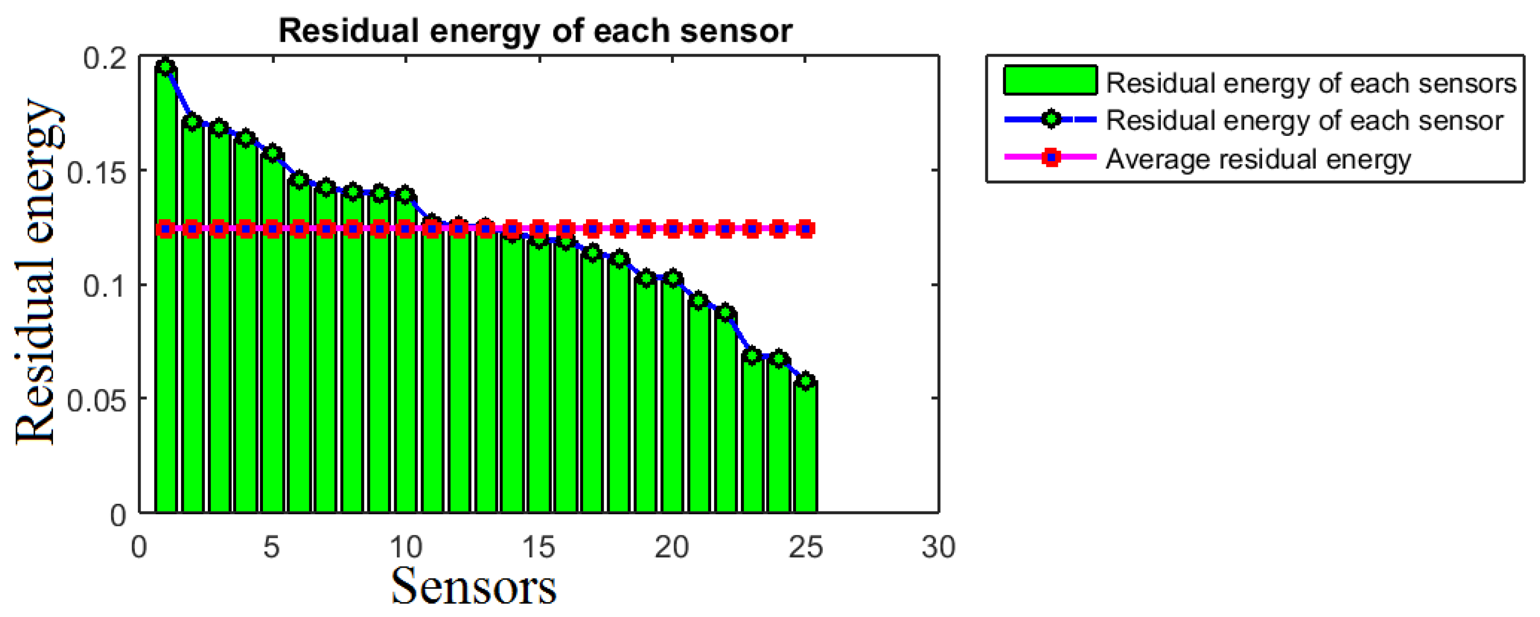
4. Simulation Results

The energy consumption obtained by each sensor is calculated and then the results are plotted. These figures are obtained, each sensor sends data to its chosen neighbour using the SRA algorithm, the sensor aggregates the data of its predecessor and sends all data to its successor. This procedure is repeated until aggregated data reaches the base station. Whole simulations depend on this coming protocol: we consider 25 nodes of wireless sensor networks arbitrarily dispersed over an area of 25 m × 25 m. The base station is in the middle. Furthermore, we neglect the effect caused by signal collision and interference in the wireless channel. On account of limited energy of nodes, during the simulations, the energy diminishes when a node sends or receives data and whenever it aggregates data. In case a node runs out of energy, it can’t send or receive data. Therefore, it will be ignored in the network in future iterations. The parameters shown in

Table 1. Radio characteristics used in our simulations.

Parameter	Value
$E_{elec}$	50 nJ/bit
$E_{fs}$	10 pJ/bit/m${}^2$
$E_{mp}$	0.0013 pJ/bit/m${}^4$
$E_0$	0.5 J
k	4000 bits
$E_{DA}$	50 nJ/bit/message
$d_0$	88 m
$\alpha$	4
$\beta$	2
$\gamma$	2
$\delta$	4
$\rho$	0.02
initial value of ${\tau }_{i,j}$	0.0001
initial value of ${\eta }_{i,j}$	0.0001

are used in our simulations.

As seen in Figure 2, we distribute the sensors in a random way and we position the base station in the middle of the surface.

We can see in Figure 3, Figure 4, Figure 5 and Figure 6 that in each iteration a node that will start the transmission is not necessarily the same; it changes from one iteration to another. If a node wants to transmit the data, it looks for its successor according to its probability, which we have seen in Equation (1); likewise, the other nodes do the same thing until the data arrive at the base station.

From iterations 1 to 15, Figure 3, we see that the minimum path is 253.2010 m and the maximum path is 369.8450 m.

From iterations 16 to 20, Figure 4, we see that the minimum path is 290.5974 m and the maximum path is 349.5204 m.

From iterations 21 to 35, Figure 5, we see that the minimum path is 262.4805 m and the maximum path is 370.5428 m.

From iterations 31 to 45, Figure 6, we see that the minimum path is 272.8723 m and the maximum path is 346.5317 m.

We see in Figure 3, Figure 4, Figure 5 and Figure 6 that the path chosen during these iterations is not always the smallest path even if the network knows the smallest way because the residual energy of the nodes has also been taken into account. The source is also not always the same because the goal of our paper is to balance the energy consumption in all the nodes.

In Figure 7, the energy consumed by each sensor increases almost equitably for all sensors.

In Figure 8, the residual energy of each sensor decreases almost equitably for all sensors.

In the Figure 9, we have increasingly sorted the energy consumption of each sensor to obtain these comparable results:

The total energy consumed by each sensor is almost identical to the average energy consumed: 0.3757 j.

In Figure 10, we have decreasingly sorted the residual energy of each sensor to obtain these comparable results:

The residual energy of each sensor is almost the same as the average residual energy: 0.1242 j, the difference between the average value and the maximum and minimum values, respectively, are: 0.07079 j and 0.06663 j.

5. Conclusions

In this article, we have proposed a Smart Routing Algorithm (SRA), and the latter establishes a dynamic routing of homogeneous wireless sensor networks; indeed, it is based on the pheromone of nodes and their probability to be chosen. At first, we have reviewed the ant colony optimization and presented our proposed algorithm using some universally used parameters to evaluate the effectiveness of a given approach. We have distributed an arbitrary 25 sensors with 0.5 j initial energy for all nodes, and we have put the sink in the middle, we have validated the proposed approach (SRA) and we have evaluated its performance based on a set of simulations. The simulations have shown that all nodes can be alive for up to 50 iterations without any dead nodes, and sent a total 1250 messages, so the consumption differences between them are very few. Then, using algorithm SRA, the wireless sensor networks will have a long lifetime.

In future work, we will use heterogeneous networks to solve this very small difference of consumption between the nodes.

References

1. Bouarafa, S.; Saadane, R.; Aboutajdine, D. Reduction of Energy Consumption in WSN Using the Generalized Pythagorean Theorem. In Proceedings of the 5th International Conference on Multimedia Computing and Systems (ICMCS), Marrakech, Morocco, 29 September–1 October 2016; p. 720. [Google Scholar]
2. Deng, Z.; Wang, G.J.; Ma, Z. A Leaping Based Routing Protocol with Load Balancing Support in Wireless Sensor Network. Chin. J. Sens. Actuators 2009, 22, 407–412. [Google Scholar]
3. Stutzle, T.; Dorigo, M. A short convergence proof for a class of ACO algorithms. IEEE Trans. Evol. Comput. 2002, 6, 358–365. [Google Scholar] [CrossRef]
4. Boondirek, A.; Triampo, W.; Nuttavut, N. A Review of Cellular Automata Models of Tumor Growth. Int. Math. Forum 2010, 5, 3023–3029. [Google Scholar]
5. Tome, T.; Drugowich de Felicio, J.R. Probabilistic Cellular Automata Describing a Biological Immune System. Phys. Rev. E 1996, 3976–3981. [Google Scholar] [CrossRef]
6. Sloot, P.; Chen, F.; Boucher, C. Cellular Automaton Model of Drug Therapy for HIV Infection. In Proceedings of the 5th International Conference on Cellular Automata for Research and Industry (ACRI 02), Geneva, Switzerland, 9–11 October 2002; pp. 282–293. [Google Scholar]
7. Bouarafa, S.; Saadane, R.; Rahmani, M.D. Study of Energy Consumption in Wireless Sensor Networks Using S-Rhombus, S-Square and S-Circle Deployment. Int. J. Adv. Res. Comput. Sci. 2017, 7, 402–410. [Google Scholar]
8. Singh, S.K.; Singh, M.P.; Singh, D.K. A Survey of Energy-Efficient Hierarchical Cluster-Based Routing in Wireless Sensor Networks. Int. J. Adv. Netw. Appl. 2010, 2, 570–580. [Google Scholar]
9. Khandani, A.E.; Abounadi, J.; Modiano, E.; Zheng, L. Cooperative Routing In Static Wireless Networks. IEEE Trans. Commun. 2007, 55, 2185–2192. [Google Scholar] [CrossRef]
10. Ibrahim, A.S.; Han, Z.; Liu, K.J.R. Distributed Energy-Efficient Cooperative Routing in Wireless Networks. IEEE Trans. Wireless Commun. 2007, 7, 3930–3941. [Google Scholar] [CrossRef]
11. Kang, I.; Poovendran, R. Maximizing Static Network Lifetime Of Wireless Broadcast Ad Hoc networks. In Proceedings of the IEEE International Conference On Communications, Anchorage, AK, USA, 11–15 May 2003; pp. 2256–2261. [Google Scholar]
12. Tsiropoulou, E.E.; Mitsis, G.; Papavassiliou, S. Interest-aware energy collection & resource management in machine to machine communications. Ad Hoc Netw. 2018, 68, 48–57. [Google Scholar]
13. Yan, J.F.; Gao, Y.; Yang, L. Ant Colony Optimization for Wireless Sensor Networks Routing. In Proceedings of the 2011 International Conference on Machine Learning and Cybernetics, Guilin, China, 10–13 July 2011. [Google Scholar]
14. Dorigo, M.; Birattari, M.; Stiitzle, T. Ant Colony Optimization. IEEE Comput. Intell. Mag. 2006, 1, 28–39. [Google Scholar] [CrossRef]
15. Ikki, S.; Ahmed, M.H. Performance Analysis of Cooperative Diversity Wireless Networks over Nakagami-m Fading Channel. IEEE Commun. Lett. 2007, 11, 334–336. [Google Scholar] [CrossRef]
16. Chang, J.H.; Tassiulas, L. Maximum Lifetime Routing in Wireless Sensor Networks. IEEE/Acm Trans. Netw. 2004, 12, 609–619. [Google Scholar] [CrossRef]
17. Heinzelman, W.B.; Chandrakasan, A.P.; Balakrishnan, H. An application-specific protocol architecture for wireless microsensor networks. IEEE Trans. Wireless Commun. 2002, 1, 660–670. [Google Scholar] [CrossRef]
Figure 1. Radio energy dissipation model, adopted from [17].
Information 09 00023 g001
Figure 2. The sink in the middle and the nodes are scattered arbitrarily.
Information 09 00023 g002
Figure 3. The constructed paths in iterations 1–15.
Information 09 00023 g003
Figure 4. The constructed paths in iterations 16–20.
Information 09 00023 g004
Figure 5. The constructed paths in iterations 21–35.
Information 09 00023 g005
Figure 6. The constructed paths in iterations: 36–50.
Information 09 00023 g006
Figure 7. Energy consumption by each node in each iteration.
Information 09 00023 g007
Figure 8. Residual energy of each sensor for 50 iterations.
Information 09 00023 g008
Figure 9. Energy consumed by each sensor for 50 iterations.
Information 09 00023 g009
Figure 10. Residual energy of each sensor for 50 iterations.
Information 09 00023 g010