Analytical Framework for Preliminary Planning of Very High-Speed Digital Subscriber Line Access Networks

Abstract

In this paper, we introduce an analytical framework for the performance evaluation of the VDSL2-based access systems. It allows for the obtaining of approximations of the achievable bit rate per user, taking into account several factors, such as the bit-loading limitation per sub-carrier; interference scenario, including the number and positions of the active interferers along the cable; crosstalk statistics; and vectoring. A closed-form expression for the maximum sub-carrier frequency that can be loaded with the maximum number of allowed bits is also presented. Formulas are obtained assuming log-normal statistics for the signal-to-interference-plus-noise ratio (SINR) per sub-carrier. The validity of the proposed formulas has been assessed by computer calculations. A very good agreement between the exact and the approximated bit rates has been obtained. The framework can be used for preliminary design of VDSL2 systems in terms of the bit rate coverage, as well as to analyze performance of other access technologies such as ADSL and G.fast.

1. Introduction

According to the Digital Agenda for Europe (DAE), by 2020, all Europeans should access the Internet at speeds greater than 30 Mbit/s, and not less than 50% of European households should be able to subscribe to contracts at speeds over 100 Mbit/s. The technology originally assumed as a baseline for the latter target of the DAE was considered to be Fiber-to-the-Home (FttH). This turned out to be a reasonable solution only in green-field deployments, where it can be delivered at a reasonable cost, but in Europe, telecommunication operators have to deal mostly with brown-field deployments in built-up, often dense urban areas. In particular, pervasive FttH deployment should have replaced copper for supporting novel ultra-broadband (UBB) services and network back-hauling. However, the very high costs (per home) of the FttH network have discouraged telecommunication operators to fully invest in FttH due to a non-favorable return of investments [1,2]. Thus, the need of UBB (such as for 4 K TV and cloud computing-based services) to their subscribers, as well as to provide back-hauling for actual and (possibly) future 5G radio access networks has led to a renewed interest in copper-based access technologies and in the related access network architectures to fully exploit their potentials. To improve achievable performance of copper, two main strategies can be followed. The first consists of the deployment of access network architectures capable of reducing the length of the copper wire to subscribers. The second focuses on the performance improvement of digital subscriber line (DSL) transmission technologies obtained with an increase of the transmission band and the adoption of techniques to reduce crosstalk.

In the last few years, the main approach toward UBB developed by most European telecommunication operators involved a careful evolutionary migration path from the presently ubiquitously deployed all-copper DSL access networks to all-optical access networks based on passive optical networks (PONs) [3]. The evolutionary strategy is implemented case-by-case using one of the possible intermediate hybrid fiber–copper access solutions, including fiber-to-the-cabinet (FttC), fiber-to-the-distribution point (FTTDp) and fiber-to-the-building (FttB), which progressively reduce the wire lengths to the subscribers. The International Telecommunication Union (ITU) has recently finalized the standardization activity for the G.fast solution [4] to be used in (future) FttDp architectures [5]. Thanks to the reduction in copper wire length for FttDp (e.g., the typical distance between the Dp and the customer premises equipment (CPE) is about 100 m), the G.fast solution will allow the use of frequency ranges up to hundreds of MHz. Depending on the cable quality, the standard will presumably exploit the twisted pair’s spectrum up to about 100 or 200 MHz, thus achieving the maximum theoretical transmission capacity greater than 1 Gbit/s [6]. However, even though the costs for FttDp deployment are lower than the costs for FttH, they can be still considerably high due to the large number of Dp’s to be deployed and connected by fiber to the back-haul/core network. Up to now, this fact limits the rapid and pervasive deployment of G.fast technology.

Very high-speed DSL type 2 (VDSL2, ITU-T G.993.2 [7]) technology in the FttC architectures is currently the (only) solution adopted by telecommunication operators to provide UBB services. Thus, during the last few years, there has been a resurgent interest by standardization organizations and by the main manufacturers to find solutions to improve VDSL2 performance. In particular, recent VDSL2 systems allow very high bit rates to be achieved, thanks to the usage of vectoring [8], which reduces the far-end crosstalk (FEXT), and/or extending the transmission band up to 35 MHz (e.g., V-plus) [9], and/or adopting advanced coding techniques to improve transmission over copper (e.g., Huawei’s SuperVector [10]). ITU has recently approved the VDSL profile 35b [11] to accommodate these new technologies.

Performance of VDLS2 is commonly expressed in terms of the statistics (i.e., mean and percentiles) of the achievable bit rate per user. Their evaluations require the knowledge of the access network geometry, the models of propagation environment, and FEXT. Simulation tools including these models are typically used by telecommunication operators to assess performance. Proper FEXT characterization is an important issue to obtain realistic results. Direct propagation channel models depend on the cabinet-to-user distance and on the copper-pair propagation characteristics. These are described by the primary and secondary constants of the cable as a function of frequency [12]. Concerning FEXT, several models (mostly based on experimental data) have been proposed by ITU [11] and other organizations/institutions, such as in [13]. The document in [11] reports the attenuation model and the FEXT model based on the 99th percentile of FEXT measurements in the cable, i.e., only $1\%$ of all pairs in all cables experience more crosstalk than the model value at the considered distance. Nevertheless, as indicated in [14], the $1\%$ worst-case assumption is acceptable for designing DSL system power spectral density (PSD) masks in order to limit the “impact” onto neighboring DSL services [15]. However, in most of the cases, this does not correspond to realistic situations, and could negatively bias any performance gain inherent to technologies aimed at avoiding and/or mitigating FEXT-dominant crosstalk. In general, these FEXT models do not reflect the wide field variation of FEXT strengths throughout the channel, and they do not account for the variation in FEXT coupling dispersion throughout the cable.

To compensate for the limitations of the $1\%$ worst-case assumption, FEXT models adding FEXT coupling dispersion with respect to the $1\%$ model have been presented in the literature. Two important examples are reported in [13,14], where FEXT dispersion (in dB) has been modeled using beta and normal distributions. Both models in [13,14] allow accounting for inter-binder interference by adding an additional attenuation factor (in dB) to FEXT fluctuations, whose value depends on the relative positions of the binders in the cable.

To further include frequency selectivity in existing FEXT models, authors in [16,17] have proposed two distinct parametric stochastic models for FEXT frequency fluctuations. Then, the overall FEXT model is obtained by multiplying the $1\%$ model, including dispersion, by the selectivity term at a frequency $f_k$ evaluated in accordance with the models in [16] or [17]. Finally, in [18], FEXT fluctuations have been modeled by the gamma distribution. This channel model is limited to $3.15$ MHz and so it is not considered in the following.

The adoption of a simulation-based approach for preliminary planning of the access network can be time consuming. To overcome this inconvenience, in this paper, we propose an analytical framework based on two approximated stochastic models for the user bit rate that can be easily implemented on any calculator. In particular, differently from [19], we introduce a novel normal stochastic model of the bit rate per user accounting for the bit-loading limitation per sub-carrier and for vectoring. A bit-loading limitation per sub-carrier is imposed by the VDSL2 standard, i.e., the number of bits per sub-carrier cannot exceed $b_{max}=15$, and cannot be lower than $b_{min}=1$. Moreover, we also present a closed-form expression for the maximum sub-carrier frequency $f_{max}$ transmitting up to $b_{max}$ bits. This formula evidences the dependence of $f_{max}$ on the FEXT statistics, on the pair-coupling characteristics, on the distance of the reference user from the cabinet, on the geometry of the interference scenario, and on vectoring. Models have been obtained starting from log-normal approximations of the signal-to-interference-plus-noise ratio (SINR) per sub-carrier introduced in [20] and further validated in [19] and these are not discussed further. The presented analytical framework facilitates the preliminary design and performance assessment of current and enhanced VDSL2 systems and other technologies, such as ADSL and G.fast (ITU G.9701). The formulas presented in this paper are valid for the downstream (DS) transmission direction only, but can be re-adapted to upstream (US). The validity of the bit rate models presented in this paper has been assessed by computer calculations. A very good agreement with the bit rate values obtained from exact calculations has been observed for variable access network topologies, interference scenarios, and for distances which are of interest for practical VDSL2 deployment.

The bit rate coverage for fixed VDSL2 networks is introduced and evaluated in this paper. It is defined as the probability the bit rate per user is greater than a reference bit rate value. Coverage is obtained after saturating over all possible positions of interferers in the access network, and over all the distances of the reference user from the cabinet. By definition, the bit rate coverage provides an indication of the percentage of users that can be served with an assigned bit rate level for the given access network configuration and cable load (i.e., the number of active copper lines), independently of the position of terminals with respect to the cabinet(s). In a practical setting, VDSL2 coverage can be evaluated by first collecting bit rate measurements from a set of VDSL2 active lines from one cabinet in the area, and then evaluating the cumulative distribution of these measurements. When more cabinets are considered, the bit rate coverage can be calculated for each cabinet separately. This means we take into account the specific propagation and interference conditions of the single cabinet, and then combine results from all the cabinets in some way (for example, by averaging). Coverage results obtained from exact calculations are compared with those obtained using the bit rate approximations presented in this paper. A very good agreement between exact and approximated results was obtained.

The paper is organized as follows. In Section 2, we describe the typical access network architecture for VDSL2 deployment, and we define the expression of the SINR per sub-carrier. The log-normal approximation of the SINR is introduced in Section 3. In Section 4, we derive the bit rate approximations, including the bit-loading limitations. The validity of the proposed models is discussed in Section 5 under variable interference scenarios. Some applications of the proposed formulation, including VDSL2 coverage, are illustrated in Section 6. Finally, conclusions are drawn.

2. Access Scenario and Performance Parameter Definition

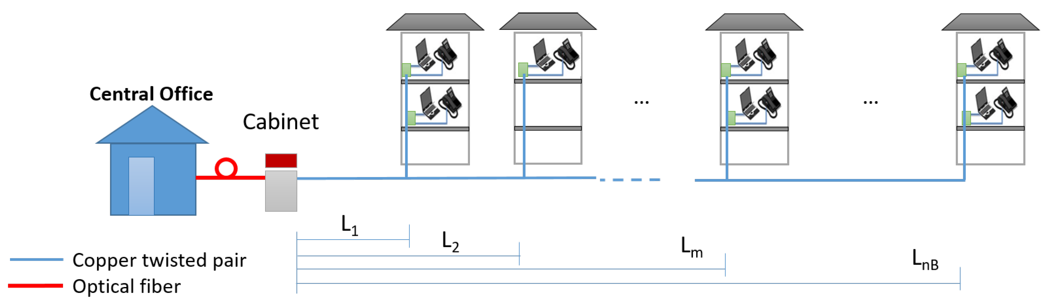
The typical geometry of FttC access networks is depicted in Figure 1.

Interferers are inside the $n_B$ buildings served by the same cable. The ith building contains $k_i$ active interferers using copper pairs in the same or in other binders inside the same cable. The typical number of copper pairs in each binder varies from 25 up to 50; the cable from the cabinet typically contains four or eight binders. As shown in Figure 1, buildings are at distances $L_i$, $i=1,2,\dots ,n_B$, from the cabinet. Active users in the same building can be randomly located on the floors. The main VDSL2 performance parameter is the bit rate achieved by a single user at distance d from the cabinet. It is defined as:

$$R_b\left(d\right)=R_s\sum _{k\in I_c}B\left[{\rho }_k\left(d\right)\right]$$

(1)

In Equation (1), $I_c$ is the set of sub-carrier indices assigned to DS transmission, $R_s$ is the symbol rate, $B[·]$ is the number of bits that can be allocated on the kth sub-carrier in accordance with the following criterion:

$$B\left[x\right]=\left\{\begin{array}{cc}{b}_{max}\hfill & \mathrm{if}x\ge b_{max}\hfill \\ x\hfill & \mathrm{if}{b}_{min}\le x<b_{max}\hfill \\ 0\hfill & \mathrm{otherwise}\hfill \end{array}\right.$$

(2)

where $b_{min}$ and $b_{max}$ are the minimum and maximum number of bits, respectively, that can be allocated per sub-carrier, and ${\rho }_k\left(d\right)$ in Equation (1) is:

$${\rho }_k\left(d\right)={log}_2\left(1+\frac{SIN{R}_k\left(d\right)}{\Gamma }\right)$$

(3)

and $\Gamma$ is the performance gap [8]. The term $SIN{R}_k\left(d\right)$ is the SINR of the kth sub-carrier at frequency $f_k$ for the reference user at distance d from the cabinet and it is defined as:

$$SIN{R}_k\left(d\right)=\frac{|H_{D,k}{\left(d\right)|}^2{P}_k}{{\eta }_k+v_{r,k}{I}_k\left(d\right)}$$

(4)

In Equation (4), $H_{D,k}\left(d\right)$ is the direct-channel transfer function at frequency $f_k$, ${\eta }_k$ is the background noise power, and $P_k$ is the power transmitted by the reference user on the kth sub-carrier. We assume DS users in the same cable use the same transmission power. This avoids harmful FEXT of high-power users on low-power users. The term $v_{r,k}$ accounts for the (possible) FEXT reduction due to vectoring [8], i.e., $v_{r,k}=1$ in the no vectoring case, and otherwise $v_{r,k}\ll 1$. The exact values of $\left\{v_{r,k}\right\}$ depend on the selected vectoring algorithm, and on its specific implementation in the DSL Access Multiplexer (DSLAM). Considering the typical vectoring algorithm indicated in [21], we have observed that $v_{r,k}$ increases with the frequency up to about $-20$ dB at 35 MHz. Finally, $I_k\left(d\right)$ is the FEXT power:

$$I_k\left(d\right)=\sum _{p=1}^{n_I}{\left|H_{F,k}^{(p,r)}\left(d\right)\right|}^2{P}_k$$

(5)

where $n_I$ is the number of interferers on the reference receiver (r); $H_{F,k}^{(p,r)}\left(d\right)$ is the FEXT transfer function at distance d accounting for the interference of the pth user; and $p=1,\dots ,n_I$, on the kth sub-carrier of the reference user. To keep notation simple, the dependence of $H_{F,k}^{(p,r)}\left(d\right)$ on the corresponding coupling length has been omitted. For DS transmissions, we have [14]:

$$|H_{F,k}^{(p,r)}{\left(d\right)|}^2={\chi }_F{f}_k^2{l}_{p,r}{10}^{\frac{X_{p,r}}{10}}{\left|H_{D,k}\left(d\right)\right|}^2$$

(6)

where $l_{p,r}$ is the coupling length between the pth interfering user and the reference user, and ${\chi }_F$ is the FEXT coupling coefficient. For assigned reference, distance d, $l_{p,r}$ can be easily obtained from the access network geometry in Figure 1. The term $X_{p,r}$ (in dB) is a random variable accounting for FEXT fluctuations with respect to the $1\%$ FEXT condition [14]. The term $X_{p,r}$ is assumed to be normal (in dB), and its mean ${\mu }_{dB}$ and variance ${\sigma }_{dB}^2$ do not depend on d. Furthermore, we consider that the $\left\{X_{p,r}\right\}$ do not vary with frequency, and are statistically independent and identically distributed (i.i.d.). From Equation (5) to Equation (6), the $SIN{R}_k\left(d\right)$ in Equation (4) is

$$SIN{R}_k\left(d\right)=\frac{D_k\left(d\right)}{1+v_{r,k}{D}_k\left(d\right){\chi }_F{f}_k^2{\displaystyle \sum _{p=1}^{n_I}}{l}_{p,r}{e}^{y_{p,r}}}$$

(7)

where $D_k\left(d\right)={\left|H_{D,k}\left(d\right)\right|}^2{P}_k/{\eta }_k$ is the signal-to-background noise ratio and the random variables $y_{p,r}=ln\left(10\right)X_{p,r}/10$ are i.i.d., having a mean of $\mu =-ln\left(10\right){\mu }_{dB}/10$ and standard deviation $\sigma =ln\left(10\right){\sigma }_{dB}/10$.

3. Log-Normal Approximation of SINR

From the Appendix, $SIN{R}_k\left(d\right)$ in Equation (7) can be approximated as

$$SIN{R}_k\left(d\right)\approx \frac{D_k\left(d\right)}{1+v_{r,k}{D}_k\left(d\right){\chi }_F{f}_k^2{N}_{r}d{e}^{{\tilde{y}}_r}},$$

(8)

where

$$N_r={\displaystyle \sum _{p=1}^{n_I}}{l}_{p,r}/d$$

(9)

is the equivalent number of interfering users. This can be easily seen in the case of co-located interferers (i.e., $l_{p,r}=d$ for each p) where we obtain $N_r=n_I$. In general, $N_r$ explicitly accounts for the positions of interfering users with respect to the reference user expressed by the coupling lengths $l_{p,r}$. In the case of the cable with $Q\ge 2$ binders, indicated with ${\Delta }_{ij}$, $i,j=1,2,\dots ,Q$, the coupling coefficient among binders [13], assuming the copper line associated to the reference user is in the first binder, $N_r$ in Equation (9) is:

$$N_r={\displaystyle \sum _{p=1}^{n_{I,1}}}{l}_{p,r}^{\left(1\right)}/d+{\displaystyle \sum _{q=2}^Q}{\displaystyle \sum _{p=1}^{n_{I,q}}}{e}^{-{\Delta }_{1q}}{l}_{p,r}^{\left(q\right)}/d,$$

(10)

where $n_{I,p}$ is the number of interferes in the pth binder and $l_{p,r}^{\left(q\right)}$ is the coupling length of the pth active user in the qth binder. The second term in Equation (10) is a sort of equivalent number of interferers due to active lines residing in the adjacent binders. This fact can be again evidenced in the co-located interferers case, yielding

$$N_r=n_{I,1}+{\displaystyle \sum _{q=2}^Q}{n}_{I,q}{e}^{-{\Delta }_{1q}}$$

(11)

From Equation (11), it is observed that thanks to the separation of binders in the cable, the total number of interferers is lower than the number of active users in the cable.

The normal random variable ${\tilde{y}}_r={\tilde{\mu }}_r+{\tilde{\sigma }}_r\nu$ in Equation (8) has a mean ${\tilde{\mu }}_r$ and standard deviation ${\tilde{\sigma }}_r$, which depend on d, and $\nu$ is a normal random variable $\mathcal{N}(0,1)$. When applying Wilkinson’s method [22], ${\tilde{\mu }}_r$ and ${\tilde{\sigma }}_r$ can be calculated as (see the Appendix):

$${\tilde{\mu }}_r=-\mu +\frac{1}{2}{\sigma }^2-\frac{1}{2}{\tilde{\sigma }}_r^2,{\tilde{\sigma }}_r^2=ln\left(1+C_r\left(e^{{\sigma }^2}-1\right)\right)$$

(12)

and

$$C_r=\frac{{\displaystyle \sum _{p=1}^{n_I}}{l}_{p,r}^2}{{\left({\displaystyle \sum _{p=1}^{n_I}}{l}_{p,r}\right)}^2}\le 1$$

(13)

The $N_r$ and $C_r$ terms are two geometrical parameters accounting for the given access network geometry characteristics. It can be shown $C_r$ is monotonically increasing with d, and its minimum is $1/n_I$. Thus, when $n_I$ increases (infinitely in the limit), the FEXT fluctuation in ${\tilde{\sigma }}_r^2$ tends to reduce. Extension of the proposed and more complex scenarios have been discussed in [20].

Due to log-normality of the denominator in Equation (8), each argument of the logarithms in Equation (1) can be approximated as

$$1+SIN{R}_k\left(d\right)/\Gamma =1+e^{w_k\left(d\right)}=e^{z_k\left(d\right)},\forall k\in I_c$$

(14)

where $z_k\left(d\right)={\mu }_{z_k}\left(d\right)+{\sigma }_{z_k}\left(d\right)(-\nu )$ is normal with a mean ${\mu }_{z_k}\left(d\right)$ and standard deviation ${\sigma }_{z_k}\left(d\right)$. Similarly, $w_k\left(d\right)$ is normal with a mean ${\mu }_{w_k}\left(d\right)$ and standard deviation ${\sigma }_{w_k}\left(d\right)$. The normal $\mathcal{N}(0,1)$ random variable $\nu$ in Equation (14) is the same as in ${\tilde{y}}_r$, and it accounts for the specific FEXT coupling situation (see Appendix). The moments of the normal random variables $\left\{y_k\right\}$, $\left\{w_k\right\}$ and $\left\{z_k\right\}$ have been obtained using Wilkinson’s method without neglecting the 1 term in Equation (14) and in the denominator of Equation (8). Results have been reported in the following formulas starting with the moments of $z_k$. By repeated application of Wilkinson’s method, we obtain (for simplicity we omit the dependence on the distance d in the following formulas):

$${\sigma }_{z_k}^2=ln\left(1+\frac{e^{2{\mu }_{w_k}+{\sigma }_{w_k}^2}\left(e^{{\sigma }_{w_k}^2}-1\right)}{{\left(1+e^{{\mu }_{w_k}+\frac{1}{2}{\sigma }_{w_k}^2}\right)}^2}\right)$$

(15)

$${\mu }_{z_k}=ln\left(1+e^{{\mu }_{w_k}+\frac{1}{2}{\sigma }_{w_k}^2}\right)-\frac{1}{2}{\sigma }_{z_k}^2$$

(16)

where ${\mu }_{w_k}=-{\mu }_{y_k}-ln\Gamma +ln{D}_k\left(d\right)$ and ${\sigma }_{w_k}={\sigma }_{y_k}$ with

$${\sigma }_{y_k}^2=ln\left(1+\frac{e^{2{\mu }_k+{\sigma }_k^2}\left(e^{{\sigma }_k^2}-1\right)}{{\left(1+e^{{\mu }_k+\frac{1}{2}{\sigma }_k^2}\right)}^2}\right)$$

(17)

$${\mu }_{y_k}=ln\left(1+e^{{\mu }_k+\frac{1}{2}{\sigma }_k^2}\right)-\frac{1}{2}{\sigma }_{y_k}^2$$

(18)

and ${\mu }_{y_k}$ and ${\sigma }_{y_k}$ are the mean and the standard deviation of the normal random variable associated to the log-normal approximation of the denominator in Equation (8). Finally, ${\mu }_k=ln\left(D_k\left(d\right)v_{r,k}{\chi }_F{N}_r{f}_k^2\right)+{\tilde{\mu }}_r$ and ${\sigma }_k={\tilde{\sigma }}_r$ for $k\in I_c$, and ${\tilde{\mu }}_r$ and ${\tilde{\sigma }}_r$ are in Equation (12). Equations (15)–(18) evidence the dependence of the bit rate statistics on the FEXT parameters $\mu$ and $\sigma$, and on the scenario geometry with $N_r$ and $C_r$. To overcome the limitations of Wilkinson’s approach [22], other methods to evaluate the log-normal parameters can be considered [23]. However, in some cases, it may be not possible to obtain closed-form expressions for the parameters of the log-normal random variable approximating the sum.

On the Suitability of Log-Normal Sum Assumption

In [20], authors discussed the suitability of log-normal sum approximation when the FEXT fluctuations were distributed in accordance with the beta distribution [13]. Assuming the parameters of the log-normal FEXT are calculated, in order to have the same mean and variance of the exponentially beta-distributed FEXT, authors have proved in [20] (by computer calculations) that the log-normal sum assumption still provides accurate results even in the beta-distributed FEXT case. This fact can be further confirmed considering the following two results presented in the literature. From [14], we can observe that Kullback–Leibler distances evaluated with normal and beta exponent assumptions are close. Furthermore, in [24], authors affirm that a log-normal distribution provides a good approximation for the sum of positive random variables under general conditions. Reasoning presented in [24] seems to be correct, despite that we believe that results in [24] should be considered as a conjecture/intuition rather than a formal proof. In fact, the paper indicates some desirable properties for a random variable to properly approximate the sum of positive random variables. The log-normal distribution owns these, but it is not clear if it is the unique distribution possessing these properties. However, the conjecture in [24] enforces the validity of the log-normal sum assumption considered in this paper. In addition, in [20], it was observed that the log-normal sum approximation of the sum of exponential beta random variables improves with the number of the summed random variables. It is out of the scope of this paper to further investigate this topic.

4. Bit Rate Approximations for Access Network Planning

From Equation (1) and using Equation (14), in the case of no bit-loading limitations per sub-carrier (e.g., theoretically $b_{max}\to \infty$), the bit rate per user can be modeled with the following normal random variable [19]:

$$R_b(d,\nu )={\overline{R}}_b\left(d\right)+{\sigma }_{R_b}\left(d\right)(-\nu )$$

(19)

whose mean ${\overline{R}}_b\left(d\right)$ and standard deviation ${\sigma }_{R_b}\left(d\right)$ are:

$$\begin{gathered} {\overline{R}}_b\left(d\right)=R_s{log}_2\left(e\right)\sum _{k\in S_c}{\mu }_{z_k}\left(d\right) \\ {\sigma }_{R_b}\left(d\right)=R_s{log}_2\left(e\right)\sum _{k\in S_c}{\sigma }_{z_k}\left(d\right) \end{gathered}$$

(20)

For convenience, the dependence of the bit rate per user on d and $\nu$ has been evidenced in Equation (19).

4.1. First Bit Rate Approximation

For a given FEXT situation (i.e., for fixed $\nu$), let $N_{\nu }$ be the index of the last sub-carrier that can be loaded with $b_{max}$ bits. Depending on the considered VDSL2 standard profile (such as the VDSL2 Profile 35b, 998E35), if we assume $N_{\nu }$ is inside the set of indices of the sub-carriers of the first DS frequency sub-band, the bit rate in Equation (1) can be approximated as:

$$R_b(d,\nu )=R_s(N_{\nu }-N_1)b_{max}+R_s\sum _{k\in {\mathcal{S}}_s}B\left[q_k\left(d\right)\right]$$

(21)

where

$$q_k\left(d\right)=\left({\mu }_{z_k}\left(d\right)+{\sigma }_{z_k}\left(d\right)·(-\nu )\right)lo{g}_2\left(e\right)$$

(22)

and $N_1\le N_{\nu }$ is the index of the first sub-carrier of the first DS sub-band. In the remainder of this section, we assume $v_{r,k}=v$ for each k, and we prove that

$$N_{\nu }=⌊\frac{1}{\Delta f}\sqrt{\frac{2^{-b_{max}}}{v{\chi }_F\Gamma N_{r}d}}{e}^{-\frac{1}{2}\left({\tilde{\mu }}_r+{\tilde{\sigma }}_r\nu \right)}⌋$$

(23)

In Equation (23), $\lfloor x\rfloor$ denotes the floor operator, $\Delta f$ is the sub-carrier spacing for the considered VDSL2 profile, and ${\mathcal{S}}_s$ is the union of the set of the DS sub-carrier indices ranging from $N_{\nu }+1$ to the end of the first DS sub-band, with the sets of indices of the sub-carriers in the remaining DS sub-bands. The operator $B[·]$ in Equation (21) is necessary to exclude the un-wanted (and inexistent) additional term in the bit rate due to sub-carriers that cannot be loaded with a number of bits lower than $b_{min}$ bits (e.g., $b_{min}$ = 1 for VDSL2). The selection of the floor operator in Equation (23) leads to a conservative estimate. Ceil or round operators may also be used for defining $N_{\nu }$. In these other cases, the bit rate may differ with respect to Equation (21) by the additional bit rate due to one sub-carrier only. This difference can be considered negligible in the case of bit rates of tens of megabits per second.

Equation (23) evidences that under high-SINR and dominant-FEXT conditions, i.e., for relatively short distances of the user from the cabinet, the maximum frequency that can be used to transmit $b_{max}$ bits per symbol is a function of the FEXT statistics (i.e., ${\tilde{\mu }}_r$ and ${\tilde{\sigma }}_r$) of the equivalent number of interferers $N_r$ and of the FEXT coupling coefficient ${\chi }_F$. The adoption of efficient transmission coding schemes can reduce the gap $\Gamma$ and then improve performance, increasing $N_{\nu }$. To obtain $N_{\nu }$ in Equation (23), we observe that in order to transmit $b_{max}\gg 1$ bits per sub-carrier, condition $SIN{R}_k\left(d\right)/\Gamma \gg 1$ holds. Furthermore, assuming a dominant FEXT, we obtain $D_k\left(d\right){\chi }_F{f}_k^2{N}_{r}d{e}^{{\tilde{y}}_r}\gg 1$, and

$$\frac{1}{\Gamma }\frac{e^{-{\tilde{y}}_r}}{v{\chi }_F{f}_k^2{N}_{r}d}\ge 2^{b_{max}}$$

(24)

For a given FEXT situation and for a fixed distance d, Equation (24) is a monotonic decreasing function of the sub-carrier frequency $f_k$. Let $f_{max}$ be the value of $f_k$ satisfying Equation (24) with equality. Inverting Equation (24) with respect to $f_{max}$, we obtain $N_{\nu }=\lfloor f_{max}/\Delta f\rfloor$ in Equation (23). Thus, the last sub-carrier that can be loaded with $b_{max}$ bits has frequency $f_k^{*}=N_{\nu }·\Delta f\le f_{max}$; $f_k^{*}$ does not account for the US and DS sub-bands, which are specific to the considered VDSL2 profile. In particular, if $f_k^{*}$ falls in the US band, the maximum DS sub-carrier that can be loaded at $b_{max}$ corresponds to the last sub-carrier in the previous DS band (if any). Otherwise, if $f_k^{*}$ lies in the US band, being the first sub-band in the VDSL2 profile, then it is never possible to transmit $b_{max}$ bits per symbol on any DS sub-carrier.

The bit rate in Equation (21) can be used to numerically evaluate the average bit rate, as well as other percentiles. However, it can be difficult to evaluate the exact expression of the probability distribution function of the bit rate in Equation (21), even when the floor operation in Equation (23) is removed. Even in this case, the bit rate in Equation (21) is given by the sum of two terms: the first being log-normal, and the second being the sum of normal random variables whose number depends on $N_{\nu }$.

4.2. Normal Approximation with Bit-Loading Limitations

An important simplification of Equation (21) can be obtained by removing the floor operation in Equation (23) and substituting $N_{\nu }$ with its mean $\overline{N}$ evaluated with respect to $\nu$. Other percentiles could be considered in the following formula instead of the mean. The expression of the mean of the log-normal can be easily obtained in closed form, that is,

$$\overline{N}=E\left\{N_{\nu }\right\}=\frac{1}{\Delta f}\sqrt{\frac{2^{-b_{max}}}{v{\chi }_F\Gamma N_{r}d}}{e}^{-\frac{1}{2}\left({\mu }_r+\frac{1}{2}{\sigma }_r^2\right)}$$

(25)

Then, we can approximate the bit rate in Equation (21) with the following normal random variable:

$$R_b(d,\nu )=R_s(\overline{N}-N_1)b_{max}+R_s\sum _{k\in {\mathcal{S}}_s^{*}}{q}_k\left(d\right)$$

(26)

where ${\mathcal{S}}_s^{*}$ is the set given by the union of the set of indices of DS sub-carriers ranging from $\overline{N}+1$ to the end of the first DS sub-band, with the set including the indices of the sub-carriers in the remaining DS sub-bands. Equation (26) provides a normal approximation of the bit rate per user. It can be observed that Equation (26) overestimates the bit rate with respect to Equation (21). In fact, when $N_{\nu }\ge \overline{N}$, some sub-carriers in the second term of Equation (26) can be loaded with a number of bits greater than $b_{max}$. This can be negligible when the number of sub-carriers at $b_{max}$ is relatively small. In the absence of vectoring, typically only sub-carriers in the first DS sub-bands can be loaded at $b_{max}=15$ or more. Furthermore, due to the removal of the operator $B[·]$ in Equation (26), the estimated bit rate also includes the (unrealistic and negligible) contribution due to sub-carriers transmitting a number of bits per symbol lower than $b_{min}=1$. As shown in the following, the normal approximation in Equation (26) provides accurate results for distances up to 400 m from the cabinet, which is well beyond the typical distances envisaged for VDSL2 practical deployment.

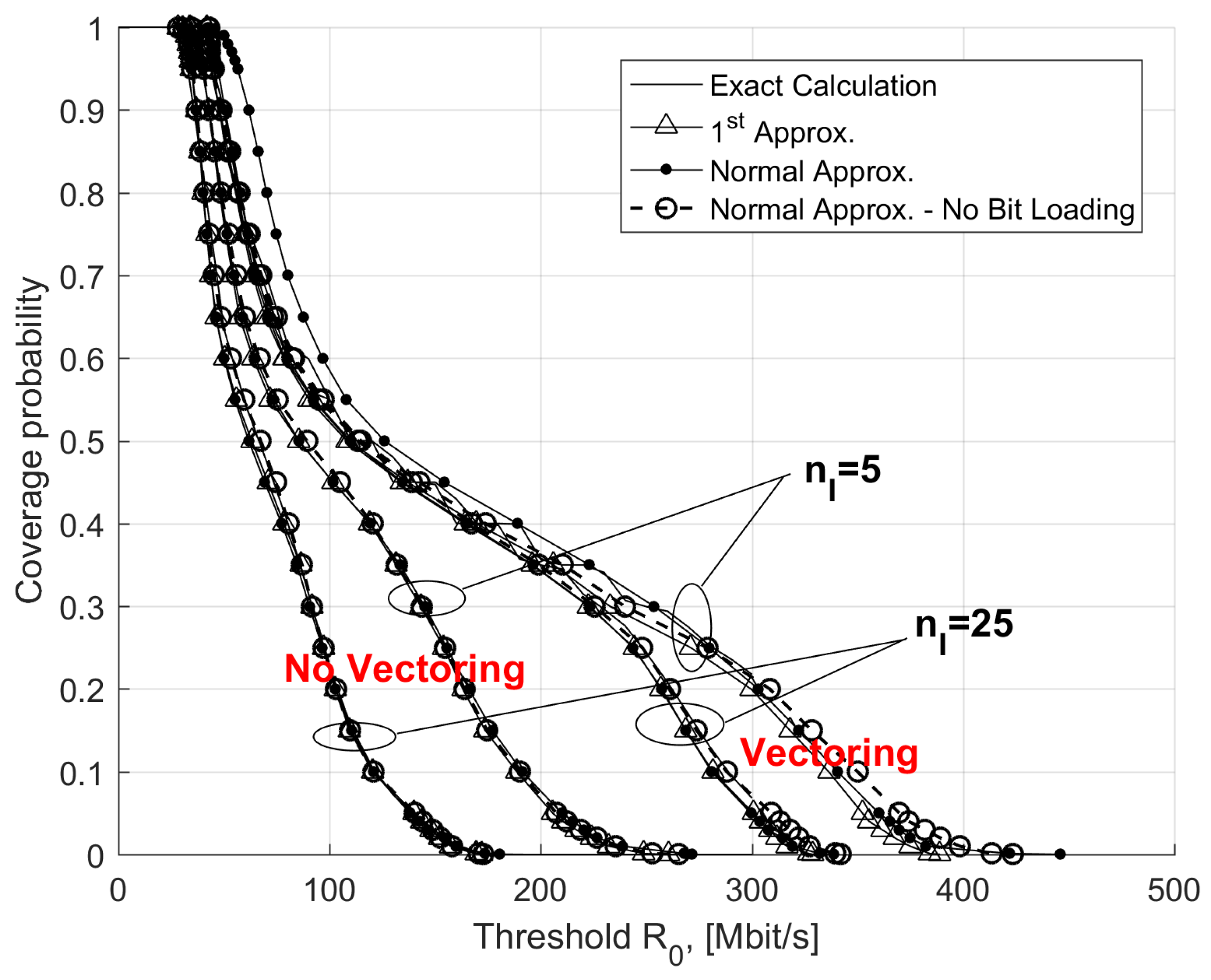
5. On the Validity of the Bit Rate Approximations

The effectiveness of the bit rate approximation in Equation (19) has been assessed in [19], and the results are not repeated here. In this section, we discuss on the validity of Equations (21) and (26) in terms of the cumulative distribution function (CDF) of the bit rate under variable interference scenarios and FEXT conditions in the non-vectored case. Vectoring is discussed in the next subsection. Results have been obtained considering co-located and uniformly distributed interferers between 50 m and 1000 m along the cable. In accordance with VDLS2 Profile 35b (998E35 [7]), we set the maximum VDSL2 frequency to $35.32$ MHz, the symbol rate is $R_s=4$ ksymbol/s, $\Delta f=4.3125$ kHz, $b_{min}=1$, $b_{max}=15$ and $N_1=32$. Moreover, the overall transmission power was $14.5$ dBm and a flat transmitter power spectrum was assumed. The FEXT coupling coefficient was ${\chi }_F\cong 3.6\times {10}^{-20}$ [25]. For validation purposes, the exact value of ${\chi }_F$ is not important. FEXT statistics are assumed to be normal, having a mean ${\mu }_{dB}$ (dB) and standard deviation ${\sigma }_{dB}$ (dB) [14]. We further assumed ${\mu }_{dB}$ and/or ${\sigma }_{dB}$ were variable, so as to assess the validity and the limitations of the considered model under different FEXT conditions.

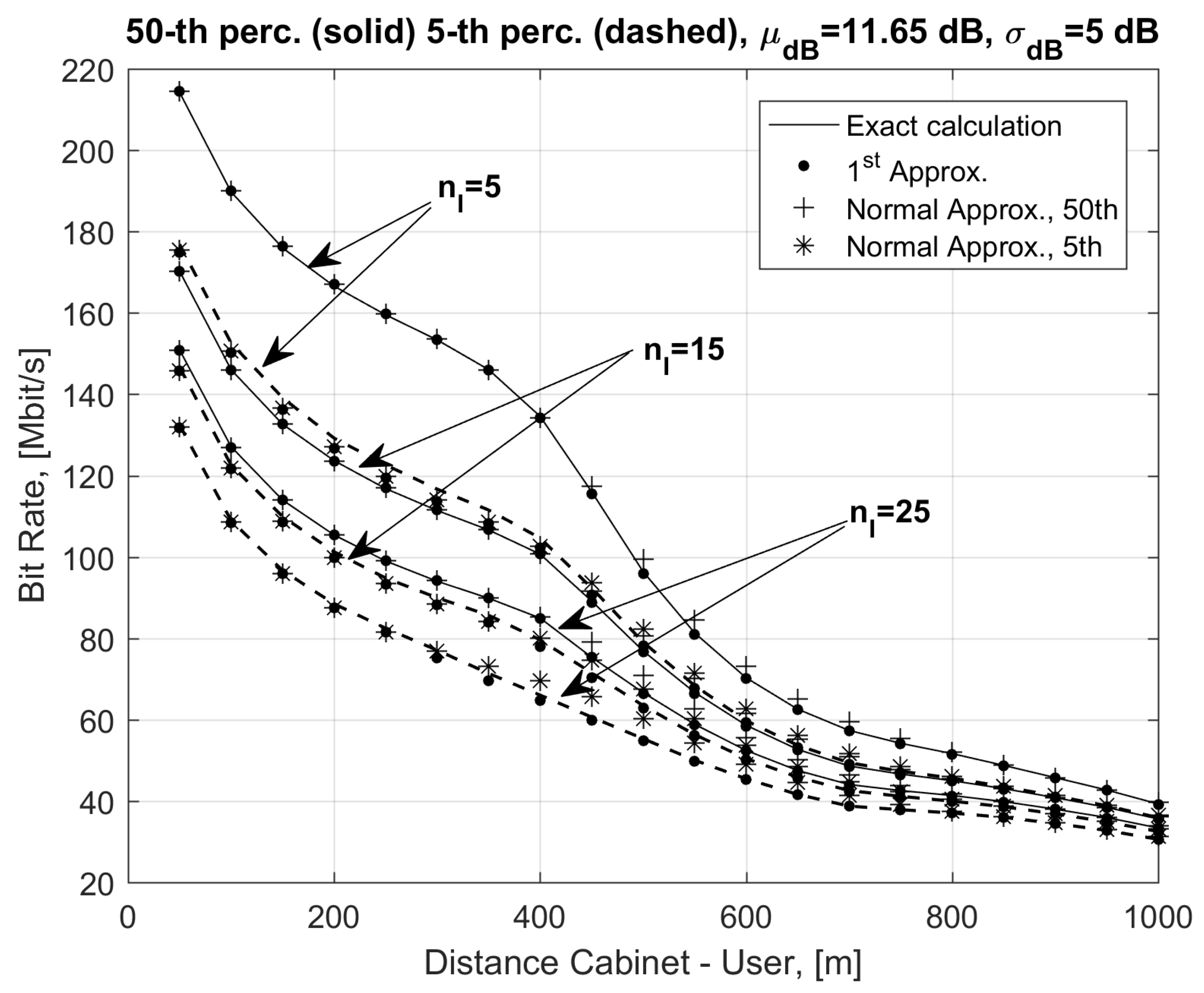
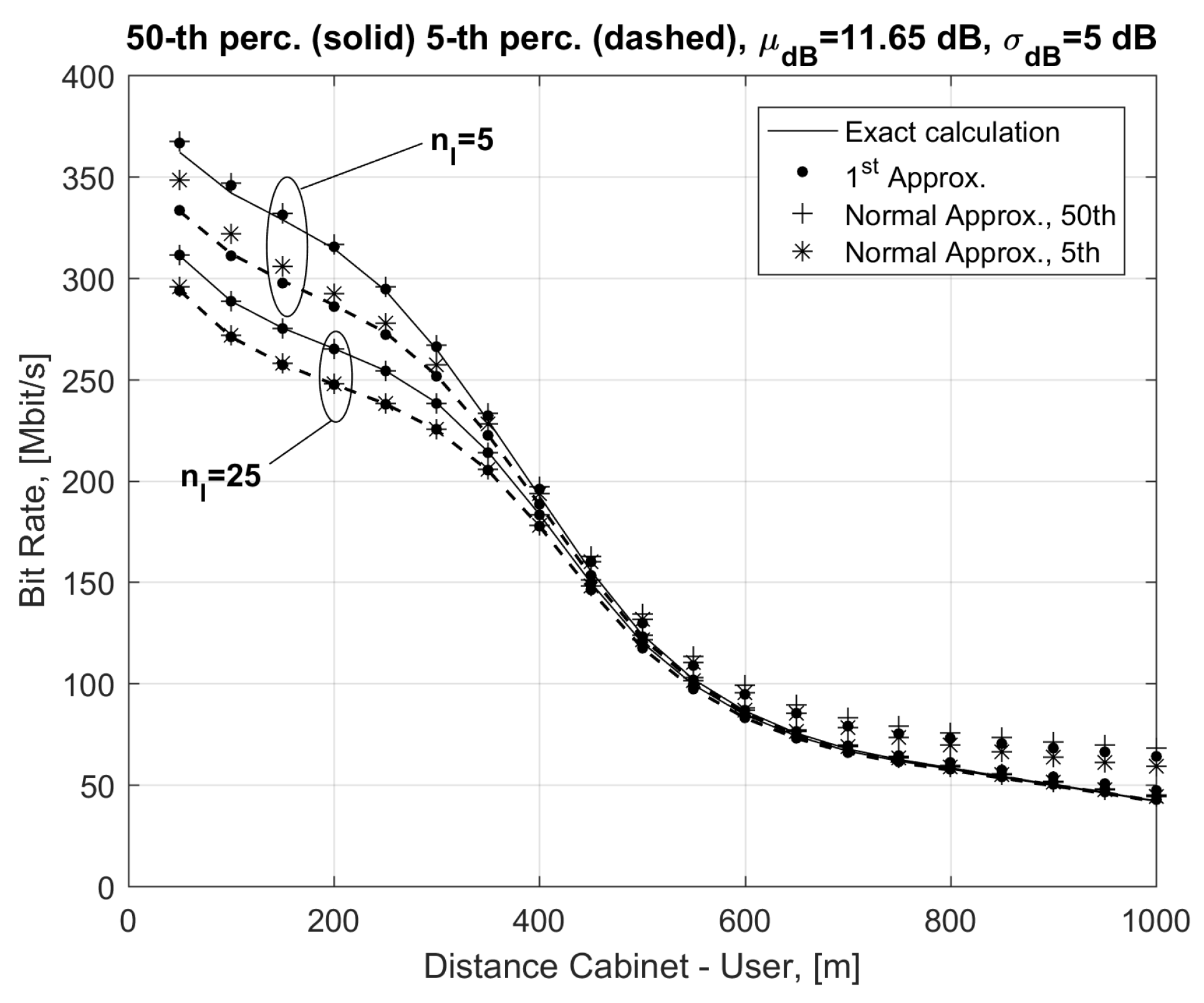
In Figure 2 we report the 5th and the 50th percentile of the bit rate as a function of the distance d of the reference user from the cabinet for variable numbers of interferers $n_I=5$, 15, 25 and a uniform distribution of the interfering users along the cable. Similar considerations applied to the co-located interferers case. Curves in Figure 2 were obtained using exact formulas in Equation (1) with the SINR in Equation (4) and FEXT as in Equation (5) (without the log-normal approximation; solid lines for the 50th and dashed lines for the 5th percentile) and the bit rate approximations in Equations (21) (with dots) and (26) (with + marks for the 50th and * marks for the 5th percentile). Results in Figure 2 show the very good agreement between the exact and approximated bit rate in Equation (21) at every distance d. Instead, the normal approximation in Equation (26) overestimates the exact results (see for example the points marked with * in Figure 2) and provides very accurate results for distances lower than 400 m and $n_I=25$.

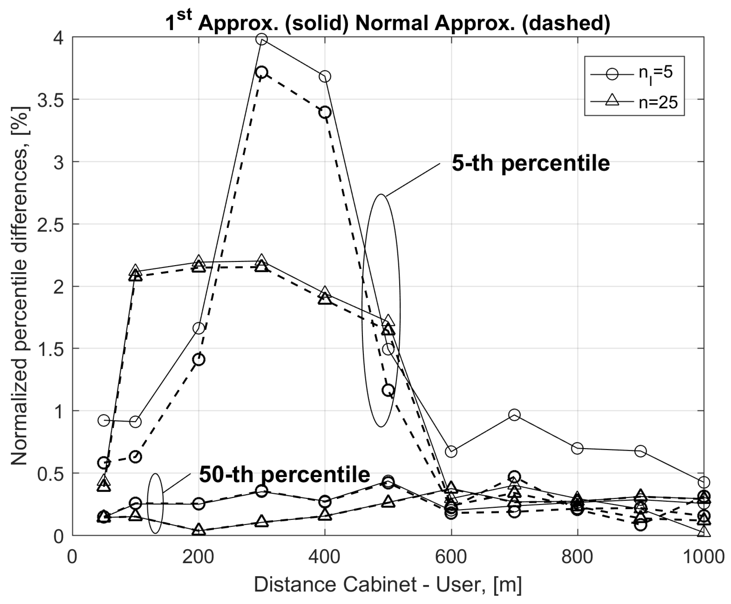
Differences between approximated bit rates are not clearly distinguishable in Figure 2. For this reason, in Figure 3, we plot the differences between the exact and the approximated values of the 50th and 5th percentiles obtained from Equations (21) (solid lines) and (26) (dashed lines). Differences have been normalized with respect to the corresponding bit rate values obtained using the exact formula in Equation (7). Differences in Figure 3 are in the order of a few percent of the bit rate, and this further confirms the validity of the considered approximations. Furthermore, results obtained with Equation (26) are closer to the exact values, as they are greater than those provided by Equation (21) for low percentiles.

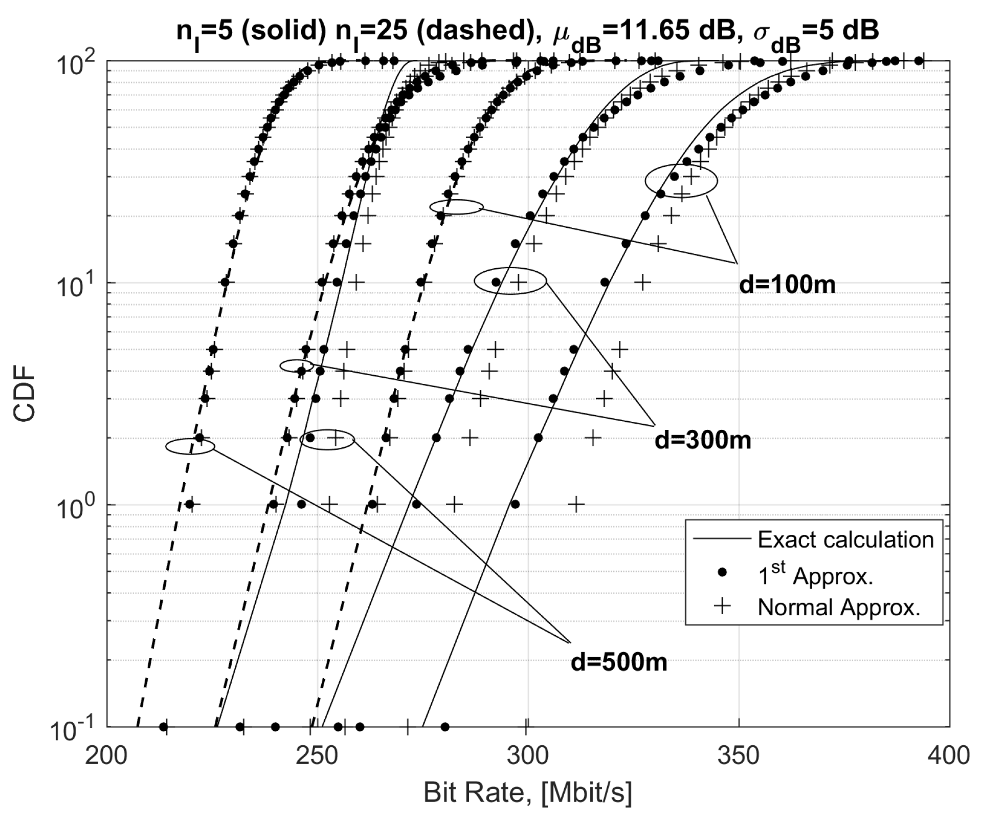
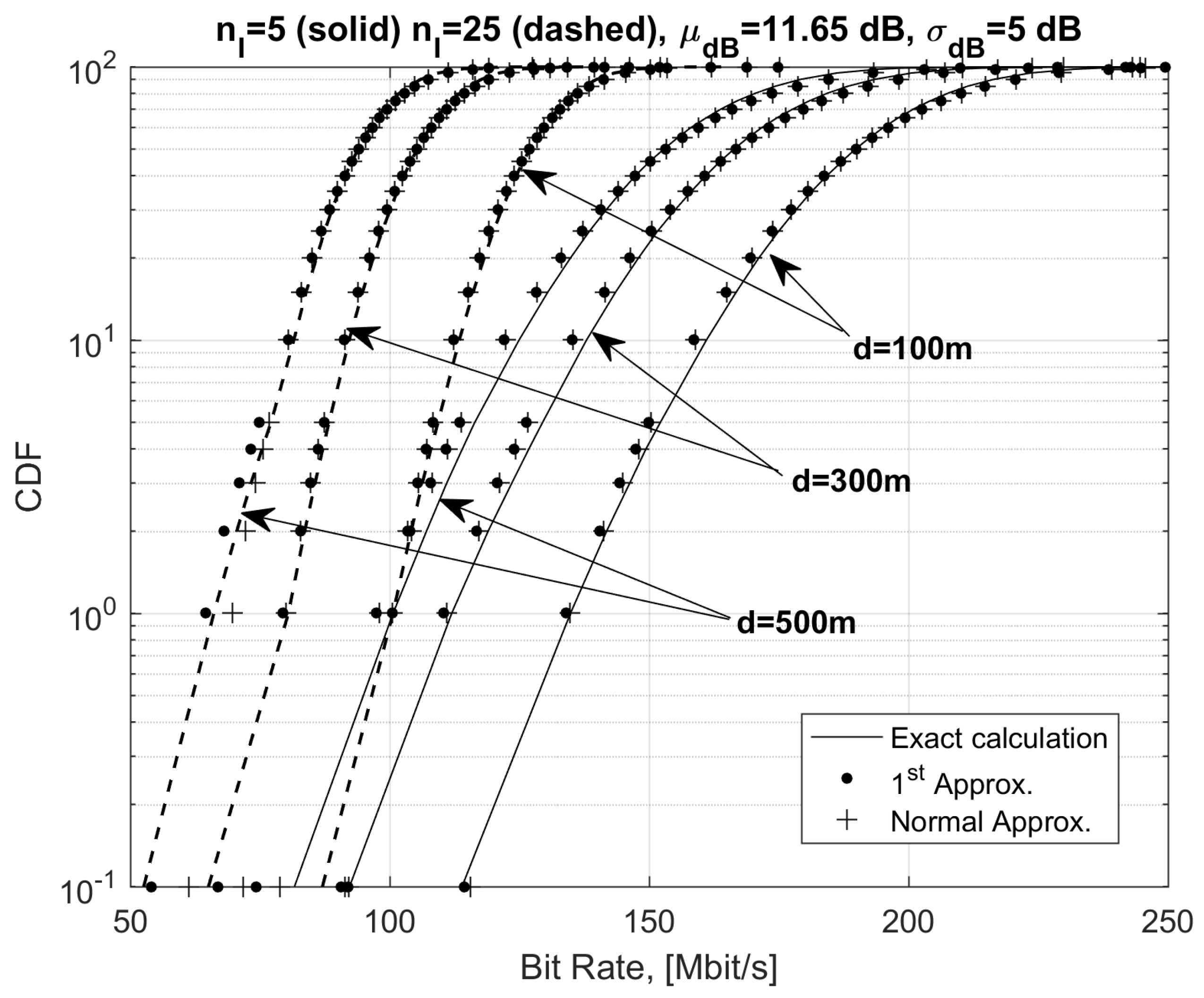
The effectiveness of Equations (21) and (26) are further confirmed by results in Figure 4 concerning the CDFs of the exact and approximate bit rates in Equations (21) and (26) for variable distance d and for $n_I=5$, 25. From Figure 4, exact and approximated CDFs are practically superimposed in all cases. As expected, the differences between Equations (21) and (26) are more evident at distances greater than 400 m, where bit rates were relatively small and the addition of an (unrealistic) term due to sub-carriers with the number of bits per symbol lower than 1 was not negligible. 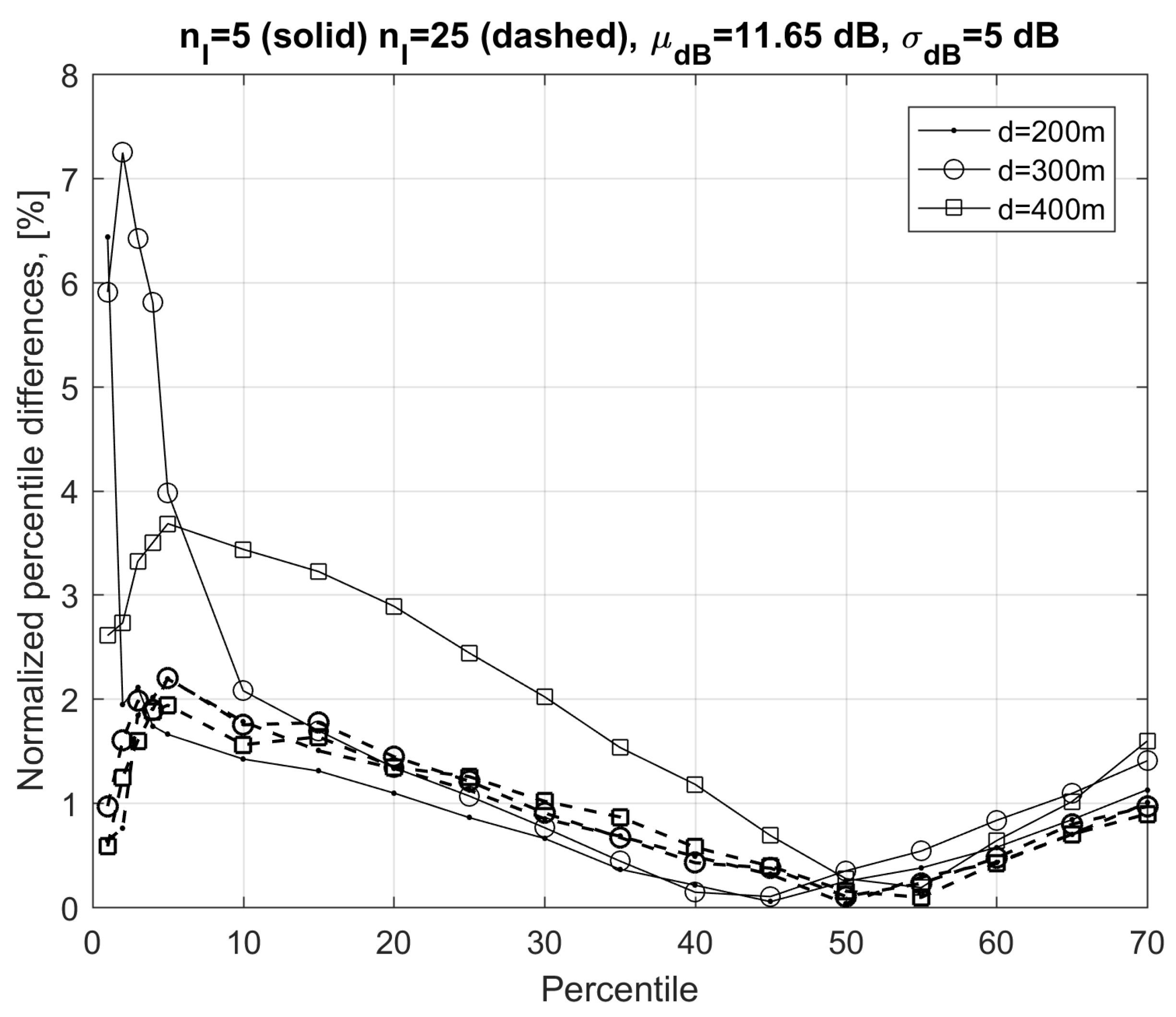Finally, by increasing distance d, the CDFs corresponding to Equation (21) tended to be closer to the exact the CDF obtained with exact calculation because FEXT becomes gradually negligible with respect to background noise. This effect is visible for distances greater than 700 m (not shown to avoid an overcrowded graph). To evidence the differences between the CDFs obtained with the exact and approximated calculations in Figure 4, in Figure 5, we plot the normalized differences among the percentiles. Differences were mostly below $4\%$ and this further confirms the validity of the proposed approximations.

The applicability of Wilkinson’s method for obtaining the statistics of the log-normal sum approximation is mainly related to the values of ${\sigma }_{dB}$ [23]. To further investigate the effectiveness of the proposed approximations, we have re-calculated the CDFs of the bit rate using Equations (21) and (26), for ${\mu }_{dB}=11.65$ dB and variable ${\sigma }_{dB}$ (dB) for some distances d and $n_I=5,25$. All results have been summarized in

Table 1. Normalized differences (in percentage) of the 5th percentile with the distance d, $n_I=5,25$ and for variable ${\sigma }_{dB}$.

	${\mathit{\sigma }}_{\mathit{dB}}$ = 4 dB				${\mathit{\sigma }}_{\mathit{dB}}$ = 5 dB
Distance (d) [m]	1st Approx.		Normal Approx.		1st Approx.		Normal Approx.
	$n_1$ = 5	$n_1$ = 25	$n_1$ = 5	$n_1$ = 25	$n_1$ = 5	$n_1$ = 25	$n_1$ = 5	$n_1$ = 25
100	0.3	0.2	0.2	0.2	1.4	0.9	1.2	0.9
200	0.9	0.1	0.8	0.1	2.5	1.1	2.2	1.1
300	1.0	0.6	0.9	0.6	2.5	2.9	2.3	0.5
500	0.2	0.1	4.3	6.1	1.4	1.1	3.8	8.8
800	0.0	0.0	1.3	1.2	0.7	0.3	0.9	1.0
	${\mathit{\sigma }}_{\mathit{dB}}$ = 6 dB				${\mathit{\sigma }}_{\mathit{dB}}$ = 7 dB
Distance (d) [m]	1st Approx.		Normal Approx.		1st Approx.		Normal Approx.
	$n_1$ = 5	$n_1$ = 25	$n_1$ = 5	$n_1$ = 25	$n_1$ = 5	$n_1$ = 25	$n_1$ = 5	$n_1$ = 25
100	3.3	3.1	2.8	3.0	6.4	8.3	5.4	7.7
200	5.1	5.1	4.6	5.0	10.3	17.7	9.2	8.7
300	6.1	11.0	5.6	5.0	17.8	17.7	12.0	6.2
500	4.8	4.9	1.9	6.1	13.2	15.0	1.8	2.6
800	2.1	1.8	0.0	0.2	4.8	4.5	1.9	2.7

, reporting the normalized differences between the 5th percentiles of the exact and approximated bit rates. Normalization of the difference was taken with respect to the corresponding exact bit rate. The results are for the variable distance d, for ${\sigma }_{dB}$ ranging from 4 dB up to 7 dB, and for $n_I=5,25$. From the results in Table 1, it is observed that the differences increased with ${\sigma }_{dB}$, and they were more than $10\%$ for ${\sigma }_{dB}=7$ at distances of about 300 m, for both approximations in Equations (21) and (26). This may render the two approximations unusable. The reduction of the normalized difference with the distance $d>700$ m for any ${\sigma }_{dB}$ was due to the FEXT decrease with the distance. In general, it has been observed that for ${\sigma }_{dB}\le 6$ dB, the approximations in Equations (21) and (26) provide accurate results, which are in very good agreement with the exact CDFs at any practical distance envisaged for VDSL2 deployment. In fact, the normalized difference of percentiles is always below $8\%$ for both Equations (21) and (26) at any distance. This also confirms results concerning the applicability of Wilkinson’s method in [23], which are accurate when ${\sigma }_{dB}\le 6$ dB. For ${\sigma }_{dB}>6$ dB, only the estimate of percentiles below $40\%$ are accurate enough. Thus, the proposed formulation based on Wilkinson’s approach can even be used to assess percentiles of CDFs ranging from $1\%$ up to $40\%$, when ${\sigma }_{dB}\ge 6$ dB. Discrepancies are due to the inability of Wilkinson’s approach to provide a good approximation for the distribution tails. In these cases, alternative methods (such as those in [23]) should be considered to evaluate the parameters of the log-normal random variable approximating the sum. Instead, for ${\sigma }_{dB}<6$, the proposed bit rate approximations in Equations (21) and (26) provide results that are in very good agreement with the exact CDFs at any practical distance (see, for example, results in Figure 4).

Validity of Formulas with Vectoring

In Figure 6, we plot the 5th and the 50th percentile of the bit rate as a function of the distance d of the reference user from the cabinet for a variable number of interferers $n_I=5,15,25$; a uniform distribution of the interfering users along the cable; and a vectoring coefficient $v_{r,k}=v=-20$ dB, assumed to be constant with frequency. This assumption is reasonable, and leads to a lower bound on the achievable bit rate with vectoring, as sub-carriers at lower frequencies may experience smaller values of v.

As expected, the achievable bit rate significantly increases with respect to the non-vectoring case. Furthermore, bit rate curves corresponding to different interfering users tend to become closer, i.e., the vectoring algorithm cancels FEXT rendering bit rate performance less sensitive to the cable load, in practice. From results in Figure 6, the approximation in Equation (21), i.e., the first approximation, is in very good agreement with the exact results for distances up to 600 m. This is well beyond the typical distances considered for VDSL2 deployment. Instead, even in this case (see discussion in the previous section), the approximation in Equation (26), i.e., the normal approximation, overestimates the bit rates at distances above 500 m.

For both approximations, a systematic error occurs in the bit rate estimate for distances greater than 600 m. This is due to the presence of the vectoring reduction factor v in Equation (23), leading to an overestimation of the number of sub-carriers that can be loaded at $b_{max}$, even when FEXT is negligible (e.g., at large distances), and the hypothesis of a dominant FEXT is no longer applicable. In order to further analyze the validity of the first and normal approximation in the vectoring case in Figure 7, we plot the CDFs of the exact and approximate bit rates in Equations (21) and (26) for variable distance d, $n_I=5$, 25 and $v=-20$ dB. In the vectoring case, the normal approximation in Equation (26) is not accurate for a small number of interfering users. Instead, it remains valid in interference scenarios characterized by medium–heavy loads (e.g., $n_I=25$) for all the distances that are of interest for VDSL2 deployment. Finally, the first approximation provides very accurate results even in the vectoring case.

6. Applications of the Proposed Formulations

After having validated the approximated bit rate formulas, now we illustrate two simple applications of Equation (23) to infer the number of bits that can be transmitted on a generic sub-carrier at frequency $f_k$ for a given interference scenario. Then, we apply the proposed formulas for evaluating the VDSL2 coverage, which can be used for network planning. Coverage results obtained using the previous bit rate approximation are compared with those obtained using exact bit rate calculations.

From now on, given the cabinet-to-user distance d, we assume the single interference scenario is specified by the number of interferers $n_I$ and their positions along the copper cable (i.e., by $N_r$ and $C_r$ in the bit rate formulas) and by the FEXT parameters ${\mu }_{dB}$ and ${\sigma }_{dB}$ (i.e., by ${\tilde{\mu }}_r$ and ${\tilde{\sigma }}_r$ in the bit rate formulas).

6.1. On the Number of Bits Per Sub-Carrier

When we assume $b_{max}$ in Equation (23) can vary from 4 up to 15, condition $SIN{R}_k\left(d\right)/\Gamma \gg 1$ holds. In this case, Equation (23) can be used to assess the corresponding maximum sub-carrier frequency $f_k\left(\nu \right)=N_{\nu }\Delta f$ that can be loaded with $b_{max}$ bits for a given $\nu$. It is well known that $99.99\%$ of the values taken by the normal $\mathcal{N}(0,1)$ random variable $\nu$ are in the interval $(-3.89,3.89)$ [26].

In

Table 2. Low and high frequencies to transmit l bits per sub-carrier for $n_I=15$.

Number of List	Low Frequency [MHz]			High Frequency [MHz]
	100 m	200 m	300 m	100 m	200 m	300 m
15	0.24	0.17	0.14	1.23	0.87	0.71
14	0.34	0.24	0.20	1.73	1.23	1.00
13	0.48	0.34	0.28	2.45	1.73	1.42
12	0.68	0.48	0.39	3.47	2.45	2.00
11	0.95	0.68	0.55	4.90	3.47	2.83
10	1.35	0.95	0.78	6.94	4.90	4.00
9	1.91	1.35	1.10	9.81	6.94	5.66
8	2.70	1.91	1.56	13.87	9.81	8.01
7	3.82	2.70	2.20	19.61	13.87	11.32
6	5.40	3.82	3.12	27.74	19.61	16.02
5	7.63	5.40	4.41	39.23	27.74	22.65
4	10.80	7.63	6.23	55.48	39.23	32.03
3	15.27	10.80	8.82	78.46	55.48	45.30
2	21.60	15.27	12.47	110.95	78.46	64.06

, we report the values of the frequencies obtained by substituting $\nu =\pm 3.89$ in Equation (23) when $b_{max}$ takes values between 4 and 15. The values in Table 2 indicate the frequencies allowed to transmit $b_{max}$ bits per symbol in accordance with FEXT coupling conditions accounted for by $\nu$ and on the distance d. In particular, considering $d=200$ m, from the results in Table 2, in the worst-case coupling condition (e.g., $\nu =-3.89$), we can transmit 15 bit per symbol on DS for frequencies ranging from 138 kHz up to 170 kHz. Instead, under more favorable coupling conditions (e.g., $\nu =3.89$) we can transmit 15 bits for sub-carriers at frequencies up to 870 kHz. The values in Table 2 do not account for the sub-bands specified in the selected VDSL2 profile. As an example, the value of the low frequency of $3.82$ MHz for $d=200$ m, corresponding to 6 bits per symbol falls in the US band of Profile 17a.

If we plot the number of bits per sub-carrier as a function of the frequencies indicated in Table 2, we obtain the “step” plot in Figure 8 corresponding to $d=200$ m. The results account for the DS-band allocation of the VDSL2 35b profile. As an example, in Figure 8, we have evidenced the two extremes of the interval corresponding to the number of bits that can be loaded on the sub-carrier at frequency $f_0=6.06$ MHz in $99.99\%$ of the cases.

6.2. Bit Rate Coverage Definition and Calculation

Starting from the proposed approximated bit rate formulas, we can derive an integral formula for the VDSL2 bit rate coverage in the absence of bit-loading limitation. The results are valid for VDSL2 systems operating over a single copper cable originating from one cabinet, but they can be extended to other and more complex situations, as detailed in the following. We assume the parameters characterizing direct propagation and FEXT statistics for the copper cable are known. In addition, the access network geometry (i.e., the links connecting users in the buildings to the copper cable) have been specified. The distance d of the reference user from the cabinet is allowed to vary between $d_{min}$ and $d_{max}$ in accordance with an assigned (continuous or discrete) probability density function $f_d\left(d\right)$, which accounts for the given access network geometry, and the positions of the buildings along the cable.

In the no-bit-loading limitation case, the bit rate per user can be approximated by Equation (19). Thus, for fixed d and for given positions of interferers along the copper cable, the probability the bit rate exceeds the threshold $R_0$ is

$$\mathrm{Prob}\left\{R_b(d,\nu )>R_0|d\right\}=1-Q\left(\frac{{\overline{R}}_b\left(d\right)-R_0}{{\sigma }_{R_b}\left(d\right)}\right)$$

(27)

where $Q(·)$ is the Q-function [26]. In the bit-loading limitation case, we adopt the approximation in Equation (26) to evaluate the coverage. After some algebra we obtain

$$\mathrm{Prob}\left\{R_b(d,\nu )>R_0|d\right\}=1-Q\left(\frac{R_s\left(\overline{N}-N_1\right)b_{max}+{\tilde{R}}_b\left(d\right)-R_0}{{\tilde{\sigma }}_{R_b}\left(d\right)}\right)$$

(28)

where ${\tilde{R}}_b\left(d\right)=R_s{\sum }_{k\in {\mathcal{S}}_s^{*}}{\mu }_{z_k}\left(d\right)$ and ${\tilde{\sigma }}_{R_b}\left(d\right)=R_s{\sum }_{k\in {\mathcal{S}}_s^{*}}{\sigma }_{z_k}\left(d\right)$.

Then, in the case of the no-bit-loading limitation per sub-carrier, the bit rate coverage conditioned to the set of distances $\left\{d_i\right\}$, $i=1,2,\dots ,n_I$, of the $n_I$ interferers from the cabinet is

$$C\left(R_0\right|{\left\{d_i\right\}}_{i=1}^{n_I},n_I)={\displaystyle \underset{d_{min}}{\overset{d_{max}}{\int }}}\left[1-Q\left(\frac{{\overline{R}}_b\left(x\right)-R_0}{{\sigma }_{R_b}\left(x\right)}\right)\right]f_d\left(x\right)dx$$

(29)

The bit rate coverage $C\left(R_0\right)$ is then obtained from Equation (29) as

$$C\left(R_0\right|n_I)=E\{C\left(R_0\right|{\left\{d_i\right\}}_{i=1}^{n_I},n_I\}$$

(30)

where the expectation in Equation (30) is taken with respect to the distances $\left\{d_i\right\}$, $i=1,2,\dots ,n_I$, of the $n_I$ interferers along the cable. An equation similar to Equation (29) can be obtained in the no-bit-loading limitation case, substituting Equation (28) for the integral in Equation (29).

In the worst-case interference scenario, i.e., $d_i=d$ for $i=1,2,\dots ,n_I$ (co-located interferers), we have $N_r=n_I$ and $C_r=1/n_I$ for each d. In this case, the bit rate coverage is given in Equation (29) (no-bit-loading limitation) and corresponds to its lowest achievable value. Thus, these two equations provide two lower bounds on the achievable area coverage.

When we consider more copper cables in the area originating from the same and/or other cabinets, bit rate coverage has to be re-calculated for each cable and for each cabinet. This means that in a planning stage, we locate the single cabinet in the area, and then we draw the path of the cable(s) from the cabinet connecting users in the buildings. Assuming a total number of active users distributed in the buildings connected to the cable (e.g., the cable load), we analytically evaluate the area coverage using Equation (29), and we determine the percentage of users that can be served with a specified bit rate $R_0$ from that cabinet. In a realistic scenario, the distance d of the reference user can assume values in the (discrete) set containing the distances of the user terminals in the buildings from the cabinet. The distances of interfering users can assume values in the same set. This allows the calculation of the integral in Equation (29) as a discrete sum. We repeat the coverage calculation for every cabinet to be positioned in the area. For planning purposes, we could assert planning is successful if all the (calculated) coverage values (or a percentage of them) are always above a specified threshold, e.g., $90\%$ (or even higher). If this condition is not met, perhaps some cabinets/cables should be re-positioned in the area, and then the coverage re-calculated. It should be noted that the interference scenario, the FEXT characteristics, the access network geometry and the distribution of the cabinet-to-user distances d can be different for each cable and for each cabinet.

In Figure 9, we report the single copper cable coverage in Equation (29) for $n_I=5,25$ in the co-located interferers scenario. A Monte Carlo approach has been used to evaluate the coverage using the bit rates evaluated with the exact formulas, and those calculated with the first approximation in Equation (21). Results have then been compared with those obtained using Equation (28), which is based on the normal approximation in Equation (26). In the same figure, we also plot the coverage obtained in the no-bit-loading limitation case, i.e., using Equation (27) in the same scenario. In the no-vectoring case, the approximated results are practically superimposed with those obtained using exact calculations. A very good agreement has been obtained with Monte Carlo-based results using both bit rate approximations. Coverage results obtained without bit-loading limitations are more optimistic at short distances (higher bit rates), despite that the results are close to those including the bit-loading limitation per sub-carrier. As expected, the coverage level reduces by increasing the number of active interfering users $n_I$ in the cable. The coverage reduction due to the bit-loading limitation is more marked for a large number of interferers (e.g., a high cable load). Instead, degradation is limited for the low-cable load case (i.e., $n_I=5$). The results in Figure 9 show that even under high-coupling FEXT conditions, telecommunication operators can safely propose commercial VDSL2 offers guaranteeing services of up to 30 Mbit/s. In fact, from Figure 9, such a bit rate can be provided to almost $100\%$ of the population, regardless of the position of the users in the access network. Thanks to vectoring, the coverage at 100 Mbit/s is increased from $20\%$ up to $50\%$ for $n_I=25$ (medium load). The results obtained from the exact calculation and those based on the first approximation are practically superimposed, while the normal approximation provides more optimistic results (about $10\%$ higher with respect to the exact results) for larger distances (i.e., small bit rates). For small distances (i.e., high bit rates), both approximations are in very good agreement with the results obtained from the exact calculations.

7. Conclusions

Starting from the log-normal approximation of the SINR per sub-carrier, we have derived an analytical framework for the approximated evaluation of the user bit rate in VDSL2 access networks. The proposed formulation can be easily applied to other DSL technologies, such as ADSL and G.fast. The framework allows us to easily account for the bit-loading limitation per sub-carrier, network topology, FEXT characteristics and vectoring. The effectiveness of the proposed formulas has been tested by computer calculations under variable FEXT conditions and different interference scenarios. A very good agreement between the approximated and exact results has been obtained. Concerning the usage of the framework equations, it has been observed that the normal approximation can be used to obtain accurate bit rate estimates and coverage results in the non-vectoring scenario. In the vectoring case, the normal approximation is sufficiently accurate only for shorter distances of the reference user from the cabinet. Instead, a first approximation provides results that are practically superimposed to the exact results in every scenario, i.e., with or without vectoring. Furthermore, it has been observed that the normal approximation without the bit-loading limitation can also be used to obtain an approximation of the area coverage, which is commonly used for access network planning.

References

1. Schneir, J.R.; Xiong, Y. Cost Analysis of Network Sharing in FTTH/PONs. IEEE Commun. Mag. 2014, 8, 126–134. [Google Scholar] [CrossRef]
2. Schindler, J.; Jaillet, J.; Toper, R.; Edwards, J. FTTH Deployment Costs: Expectations vs. Reality. Available online: http://www.ftthcouncil.eu/documents/Reports/2016/WhitePaper-FTTHRolloutCostIndicators.pdf (accessed on 17 July 2017).
3. Gaudino, R.; Giuliano, R.; Mazzenga, F.; Valcarenghi, L.; Vatalaro, F. Unbundling in current broadband and next-generation ultra-broadband access networks. Fiber Integr. Opt. 2014, 3, 129–148. [Google Scholar] [CrossRef]
4. ITU. ITU-T G.9701 Fast Access to Subscriber Terminals (G.fast)—Physical Layer Specification; Recommendation ITU-T G.9701; ITU: Geneva, Switzerland, 2014. [Google Scholar]
5. Ödling, P.; Magesacher, T.; Höst, S.; Börjesson, P.O.; Berg, M.; Areizaga, E. The fourth generation broadband concept. IEEE Commun. Mag. 2009, 1, 62–69. [Google Scholar] [CrossRef]
6. Van den Brink, R.F.M. Enabling 4GBB via Hybrid-FttH, the Missing Link in FttH Scenarios; Broadband Forum: Fremont, CA, USA, 2014; Available online: http://www.joepeesoft.com/Public/DSL_Corner/Docs/Presentations/PUB_2010_12_V01_BBF_SPACS _4GBB_via_Hybrid_FTTH_Brink.pdf (accessed on 17 July 2017).
7. ITU. ITU-T G.993.2 Very High Speed Digital Subscriber Line Transceivers 2 (VDSL2); Recommendation ITU-T G.993.2; ITU: Geneva, Switzerland, 2016. [Google Scholar]
8. Ginis, G.; Cioffi, J.M. Vectored transmission for digital subscriber line systems. IEEE J. Sel. Areas Commun. 2002, 5, 1085–1104. [Google Scholar] [CrossRef]
9. Russell, K.; Spruyt, P.; Vanhastel, S. Vplus Gets More Out of VDSL2 Vectoring. Available online: https://techzine.alcatel-lucent.com/vplus-gets-more-out-vdsl2-vectoring (accessed on 17 July 2017).
10. Huawei SuperVector: 3 Times of VDSL2 Vectoring. Available online: http://www.huawei.com/uk/solutions/broader-smarter/hw-399702-supervector-vectoring-fttc.htm (accessed on 17 July 2017).
11. ITU. ITU-T G.993.2 Very High Speed Digital Subscriber Line Transceivers 2 (VDSL2): Amendment 1; Recommendation ITU-T G.993.2; ITU: Geneva, Switzerland, 2015. [Google Scholar]
12. Werner, J.J. The HDSL environment. IEEE J. Sel. Areas Commun. 1991, 9, 785–800. [Google Scholar] [CrossRef]
13. ATIS. ATIS Multiple Input Multiple Output Crosstalk Channel Model; ATIS Technical Report NIPP-NAI-2009-014R3; Alliance for Telecommunications Industry Solutions: Washington, DC, USA, 2009. [Google Scholar]
14. Sorbara, M.; Duvaut, P.; Shmulyian, F.; Singh, S.; Mahadevan, A. Construction of a DSL-MIMO Channel Model for Evaluation of FEXT Cancellation Systems in VDSL2. In Proceedings of the IEEE Sarnoff Symposium, Princeton, NJ, USA, 30 April–2 May 2007; pp. 1–6. [Google Scholar]
15. Galli, S.; Kerpez, K.J. Methods of Summing Crosstalk From Mixed Sources-Part I: Theoretical Analysis. IEEE Trans. Commun. 2002, 3, 453–461. [Google Scholar] [CrossRef]
16. Xu, W.; Schroeder, C.; Hoeher, P.A. A Stochastic MIMO Model for Far-End Crosstalk in VDSL Cable Binders. In Proceedings of the ICC ’09, IEEE International Conference on Communications, Dresden, Germany, 14–18 June 2009; pp. 1–5. [Google Scholar]
17. Cioffi, J.M.; Fang, J.L.; Ginis, G. MIMO Model for Copper Cable: Quantitative Analysis of Matching to Measured Data. IEEE 802.3 Ethernet in the First Mile Task Force. Available online: http://www.ieee802.org/3/efm/public/mar02/fang_1_0302.pdf (accessed on 17 July 2017).
18. Lin, S.H. Statistical Behavior of Multipair Crosstalk. Bell Syst. Tech. J. 1980, 6, 955–974. [Google Scholar] [CrossRef]
19. Mazzenga, F.; Giuliano, R. Analytical Performance Evaluation of VDSL2. IEEE Commun. Lett. 2017, 1, 44–47. [Google Scholar] [CrossRef]
20. Mazzenga, F.; Giuliano, R. Log-normal Approximation for VDSL Performance Evaluation. IEEE Trans. Commun. 2016, 12, 5266–5277. [Google Scholar] [CrossRef]
21. ITU. ITU-T, G.993.5 : Self-FEXT Cancellation (Vectoring) for Use with VDSL2 Transceivers Recommendation ITU-T G.993.5; ITU: Geneva, Switzerland, 2016. [Google Scholar]
22. Beaulieu, N.C.; Abu-Dayya, A.A.; McLane, P.J. Estimating the distribution of a sum of independent log-normal random variables. IEEE Trans. Commun. 1995, 12, 2869–2873. [Google Scholar] [CrossRef]
23. Schwartz, S.C.; Yeh, Y.S. On the distribution function and moments of power sums with lognormal components. Bell Syst. Tech. J. 1982, 7, 1441–1462. [Google Scholar] [CrossRef]
24. Mazmanyan, L.; Ohanyan, V.; Trietsch, D. The Lognormal Central Limit Theorem for Positive Random Variables. Available online: http://faculty.tuck.dartmouth.edu/images/uploads/ faculty/principles-sequencing-scheduling/LognormalCLT.pdf (accessed on 17 July 2017).
25. Van den Brink, R.G. Fast: Far-End Crosstalk in Twisted Pair Cabling; Measurements and Modelling; emporary Document 11RV-022; ITU-T-SG15; ITU: Geneva, Switzerland, 2011. [Google Scholar]
26. Papoulis, A.; Pillai, S.U. Probability, Random Variables and Stochastic Processes, 4th ed.; McGraw-Hill: New York, NJ, USA, 2002. [Google Scholar]
Figure 1. Considered fiber-to-the-cabinet (FttC) generic interference scenario.
Information 08 00086 g001
Figure 2. Bit rate vs cabinet-to-user distance for n I = 5 , n I = 15 and n I = 25 (50th and 5th percentile).
Information 08 00086 g002
Figure 3. Differences (normalized to the bit rate) between the 50th and 5th percentile, obtained with the two approximations with respect to the exact values.
Information 08 00086 g003
Figure 4. Cumulative distribution function (CDF) of the bit rate for variable distance d and n I = 5 , 25.
Information 08 00086 g004
Figure 5. Normalized differences among percentiles (percentage of the corresponding bit rate).
Information 08 00086 g005
Figure 6. Bit rate vs cabinet-to-user distance for n I = 5 , n I = 15 and n I = 25 (50th and 5th percentile).
Information 08 00086 g006
Figure 7. CDF of the bit rate for variable distance d and n I = 5 , 25 .
Information 08 00086 g007
Figure 8. Number of bits per sub-carrier as a function of the frequency; VDSL2 profile 35b has been considered.
Information 08 00086 g008
Figure 9. Exact and approximated bit rate coverage with and without vectoring.
Information 08 00086 g009