Abstract
In nature, the mechanical properties of geological bodies are very complex, and its various mechanical parameters are vague, incomplete, imprecise, and indeterminate. In these cases, we cannot always compute or provide exact/crisp values for the joint roughness coefficient (JRC), which is a quite crucial parameter for determining the shear strength in rock mechanics, but we need to approximate them. Hence, we need to investigate the anisotropy and scale effect of indeterminate JRC values by neutrosophic number (NN) functions, because the NN is composed of its determinate part and the indeterminate part and is very suitable for the expression of JRC data with determinate and/or indeterminate information. In this study, the lower limit of JRC data is chosen as the determinate information, and the difference between the lower and upper limits is chosen as the indeterminate information. In this case, the NN functions of the anisotropic ellipse and logarithmic equation of JRC are developed to reflect the anisotropy and scale effect of JRC values. Additionally, the NN parameter ψ is defined to quantify the anisotropy of JRC values. Then, a two-variable NN function is introduced based on the factors of both the sample size and measurement orientation. Further, the changing rates in various sample sizes and/or measurement orientations are investigated by their derivative and partial derivative NN functions. However, an actual case study shows that the proposed NN functions are effective and reasonable in the expression and analysis of the indeterminate values of JRC. Obviously, NN functions provide a new, effective way for passing from the classical crisp expression and analyses to the neutrosophic ones.
1. Introduction
According to the shear strength formula given by Barton [1] in 1973, the joint roughness coefficient (JRC) obtained effectively is quite a crucial parameter for determining the shear strength in rock mechanics. Various methods for determining the JRC values have been proposed by many scholars [2,3,4,5,6,7,8,9,10] since Barton [11] firstly introduced the concept of JRC. Since then there have also been many studies about the anisotropy and scale effect, which are two important characteristics of JRC in the sample sizes and measuring orientations. Barton and Bandis [12] proposed that the scale effect of roughness coefficient is one of the main reasons for the scale effect of mechanical behavior of rock mass through model test studies. Du et al. [13] found that the undulation amplitudes implied the negative scale effect and presented a good logarithmic function relationship with alternation sizes. Recently, Chen et al. [14] used the digital image processing (DIP) technique to retrieve the joint surface topography and a variogram function for characterizing the anisotropy of the joint surface roughness and to estimate the joint aperture. However, existing research methods can only deal with the determinate/crisp function expressions of JRC values and analyze their anisotropy and size effect, but cannot express and handle the incomplete, uncertain, and imprecise data of JRC. Due to the incompleteness of our observations, measurements, and estimations, or the existing disturbances and uncertainties in the real world, we cannot always compute or provide exact/crisp values for the inhomogeneity of the rock joints, but we need to approximate them in indeterminate environments. In this case, Ye et al. [15] established neutrosophic functions (interval functions) of JRC and shear strength. However, they only gave the interval/thick functions of JRC and shear strength, but cannot express such an indeterminate function containing coefficients and/or parameters of neutrosophic numbers (NNs).
In fact, there always exists determinate and indeterminate information in the real world. Hence, Smarandache [16,17,18] firstly introduced the concept of NN, which is really suitable for expressing determinate and/or indeterminate information, denoted as z = a + bI. Obviously, the NN z consists of its determinate part a and its indeterminate part bI, where a and b are real numbers and I denotes the indeterminacy. Clearly, NN is more suitable for the expression of determinate and/or indeterminate information in the real world. In recent years, Ye [19] firstly proposed a multiple attribute group decision-making method under a NN environment and developed the possibility degree ranking method for ranking alternatives. Then, Ye [20] presented a bidirectional projection model of NNs for multiple attribute group decision-making problems with NN information. Further, Kong et al. [21] and Ye [22] proposed the cosine similarity measure of NNs for the misfire fault diagnosis of gasoline engines and the exponential similarity measure of NNs for the fault diagnosis of steam turbines under a NN environment. Additionally, Chen and Ye [23] introduced a projection model of NNs for the multiple attribute decision-making problem of clay-brick selection under a NN environment. Further, Liu and Liu [24] presented a NN generalized weighted power averaging operator and applied it to multiple attribute group decision-making under a NN environment. Ye [25] presented a NN linear programming method for NN linear programming problems under an indeterminate environment. All of these studies have shown the superiority of NNs to express indeterminate information. Unfortunately, NN functions have not been studied and applied in rock mechanics thus far. Hence, this original study will establish NN operations and NN functions of JRC with determinate and/or indeterminate information to express and analyze the anisotropy and scale effect of indeterminate JRC values and their changing rates in measuring sizes and orientations of test samples by the actual case of the natural joint surface sample obtained from Changshan County of Zhejiang province in China. In the real world, we cannot always compute or provide determinate/crisp JRC values for the JRC characteristics, but we can approximate them to realize the indeterminate expression and analysis of JRC values. In this case, the NN functions provide an effective mathematical tool for passing from the classical crisp expression and analysis to the neutrosophic ones.
The rest of this paper is organized as follows: Section 2 presents some basic concepts and operations of NNs; Section 3 introduces the JRC data acquisition of natural rock joint surfaces with an actual case; In Section 4, some elliptic equations with NNs (elliptic NN functions of JRC) are introduced for the descriptions of the joint profiles in various orientations and their changing rates are discussed by their derivative functions, and then the NN parameter ψ is defined to quantify the degree of the anisotropy; In Section 5, logarithmic equations containing NNs (logarithmic NN functions of JRC) are presented to analyze the JRC values and the changing rates in differently-sized joint samples; Section 6 introduces a two-variable NN function of JRC to describe JRC values in various orientations and sizes and discusses its changing rates by its partial derivative functions; Section 7 gives discussion; Finally, conclusions and future work are given in Section 8.
2. Some Basic Concepts and Operations of NNs
The concept of NN was firstly proposed by Smarandache [16,17,18], which consists of a determinate part and an indeterminate part. Then, it is denoted as z = a + bI, where a and b are real numbers and I is the indeterminacy, implying some indeterminate range I ϵ [IL, IU]. It is obvious that it can describe determinate and/or indeterminate information.
For example, assume that a NN is z = 8 + 5I, where I ϵ [0, 0.5]. Thus, its determinate part is 8, its indeterminate part is 5I, and then there is z ϵ [8, 10.5] for I ϵ [0, 0.5]. Furthermore, one can also specify some indeterminate range I ϵ [IL, IU] to satisfy the actual applied requirements.
Let z1 = a1 + b1I and z2 = a2 + b2I be two NNs for I ϵ [IL, IU]; their operational relations are given as follows [25]:
3. JRC Data Obtained from an Actual Case
In real situations, we choose a natural joint surface sample to collect data from Changshan County of Zhejiang province in China as an actual case. The foliated slate rock is grayish, completed, and hard and has a dense structure. Its surface undulates from 1 cm to 2 cm and is lightly weathered. Then, a simple mechanical hand profilograph invented by Du [26] was employed to record the surface profiles by every interval of 15° in [0°, 360°] along the specified lines. Then, we intercepted samples from 10 cm to 100 cm at an interval of 10 cm in every orientation. Finally, we use the models proposed by Zhang et al. [27] to calculate the JRC values of each samples in different sizes and directions. By the statistical analysis of all JRC values of every sample, we can obtain the average values and standard deviations of all sizes in each direction, which are used in the following case analyses.
4. NN Functions for Describing the Anisotropic Characteristics of JRC
4.1. NN Functions of JRC in All Orientations
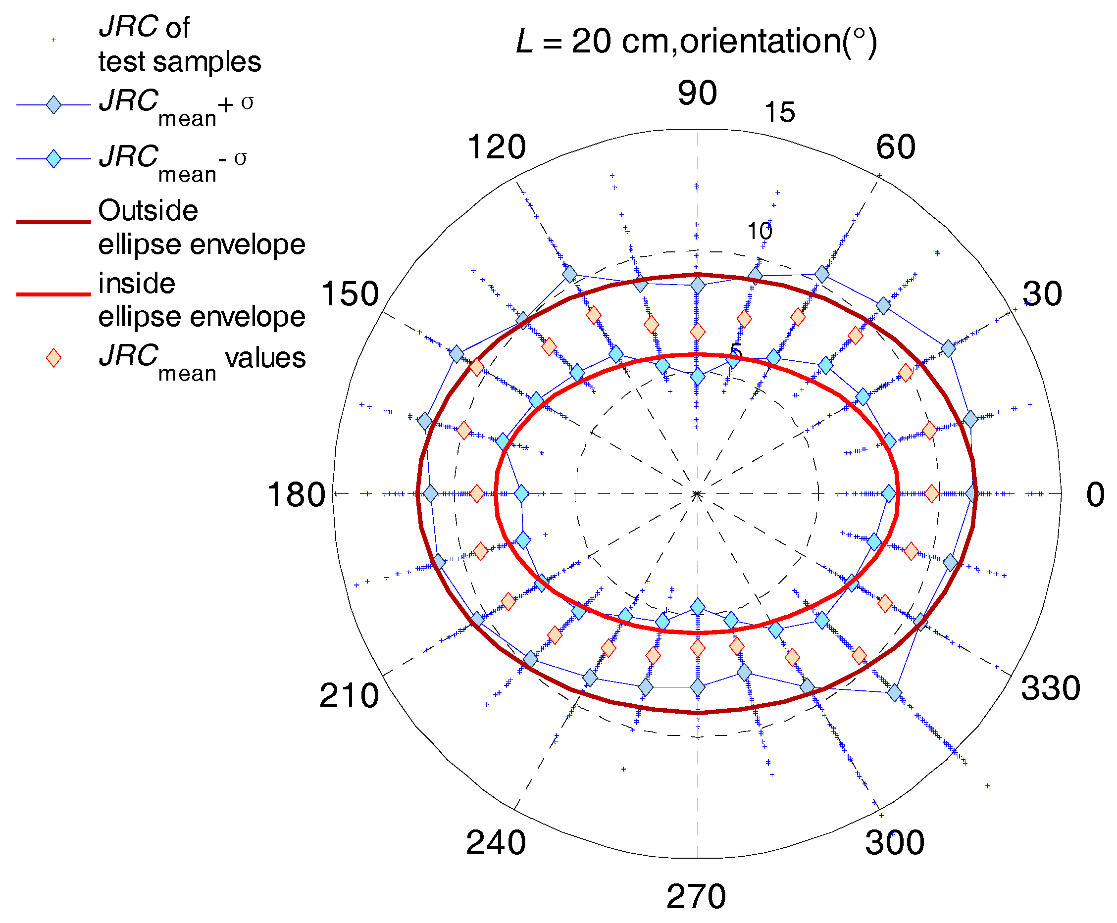
Here, we take a sample in the length of 20 cm as an example. All measured values and the mean values of JRC in every orientation on one polar plot are shown in Figure 1. It can be found that the JRC values are randomly distributed from 0 to 20 in each orientation. Then, the JRC values in the orientations of 90° and 270° are smaller, while the JRC values in some orientations such as 0° and 180° are relatively greater. Performing a calculated analysis, the JRC average value and variance of each angle orientation are obtained by the statistical analysis. For example, the average value JRCmean and standard deviation σ of JRC values for 20 cm joint samples in the 0° orientation are 9.653 and 1.716, respectively. The smaller standard deviation indicates that the data points tend to the mean value.
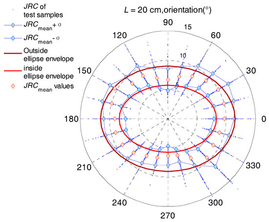
Figure 1.
Polar plots of directional JRC values, upper and lower limits of JRC values and the corresponding ellipse fitting envelopes of 20 cm joint samples.
According to the statistical analysis, about 70% of the points focus on one area in Figure 1, then most of the blue stars are crowded together. Hence, we may choose a robust range (confidence range) from JRCmean − σ(lower limit) to JRCmean + σ(upper limit) for describing the anisotropic characteristics. In Figure 1, it is shown that these upper and lower limits can be approximately structured as one ellipse area. It is obvious that the JRC mean values and most of the sample data fall into the area between two red ellipses.
Based on the least square method, the upper and lower limits of JRC values are fitted by two ellipse envelopes for joint samples of each size. Then, according to the concept of NNs and the general parametric equations of the ellipse, the NN parametric equations of JRC can be written as:
where a1 and a2 are two radiuses of the inside ellipse envelope, and a1 + b1I and a2 + b2I are two radiuses of the outside ellipse envelope. Through the statistical analysis of all sizes, the indeterminacy I belongs to the interval [0, 0.5]. Then, bi (i = 1, 2) can be determined by the twice of the difference between the radii of the inside and outside ellipse envelopes.
Each JRC value in Figure 1 is the distance from any point within the two ellipses to the coordinate origin. To express the JRC values in any orientation, by using Equations (3) and (5) we can derive the following NN function:
In order to reflect the changing rate of JRC(θ) in any orientation; here, we carried on the derivative operation of Equation (6) and obtain the following derivative Equation (7) so as to analyze the variation situations of anisotropy:
For example, when the length L = 20 cm in Figure 1, the NN parametric equations with I ϵ [0, 0.5] can be obtained by the following steps:
Thus, we have the following NN function with I ϵ [0, 0.5]:
Thus, its NN derivative function with I ϵ [0, 0.5] is given as follows:
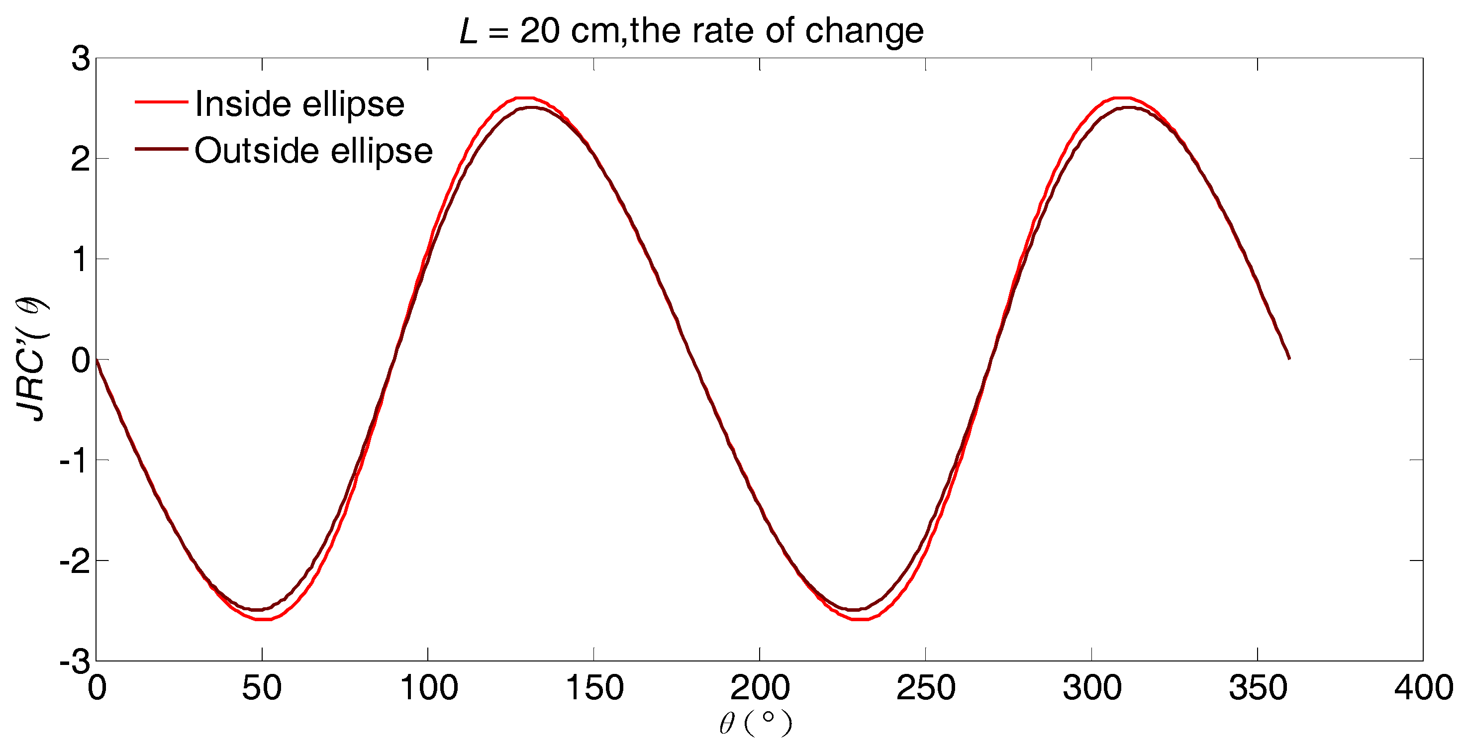
The changing rate of JRC’(θ) is shown in Figure 2. It is obvious that the changing curves of the inside and outside ellipse envelopes present periodicity and the changing rates fall into the range between two negative sine functions.
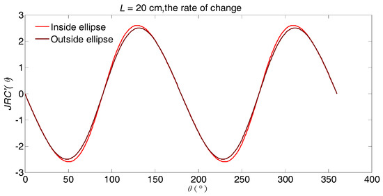
Figure 2.
The changing curves of the lower and upper limits for JRC’(θ).
By the similar method, we can obtain the NN functions of JRC(θ) and JRC’(θ) with I ϵ [0, 0.5] and various scales. Then, all of the results are shown in Table 1 and Table 2.

Table 1.
NN functions of JRC(θ) for the JRC expressions of different sized joint samples and I ϵ [0, 0.5].

Table 2.
NN functions of JRC’(θ) of different sized joint samples and I ϵ [0, 0.5].
4.2. Anisotropic Parameter
In 2009, Tatone [28] defined a parameter to quantify the anisotropy that is the ratio of the maximum directional roughness to the minimum directional roughness on the polar plots. Based on the anisotropic definition, we present the NN anisotropic parameter to characterize the degree of anisotropy for each size. Here, the maximum directional roughness is the semi-major axis of ellipse; the minimum directional roughness is the semi-minor axis of the ellipse. Hence, the NN anisotropic parameter is defined as the following form:
Then, according to the Equation (4), the anisotropic parameter ψ is calculated by the following formula:
For example, when L = 20 cm, we have the following result:
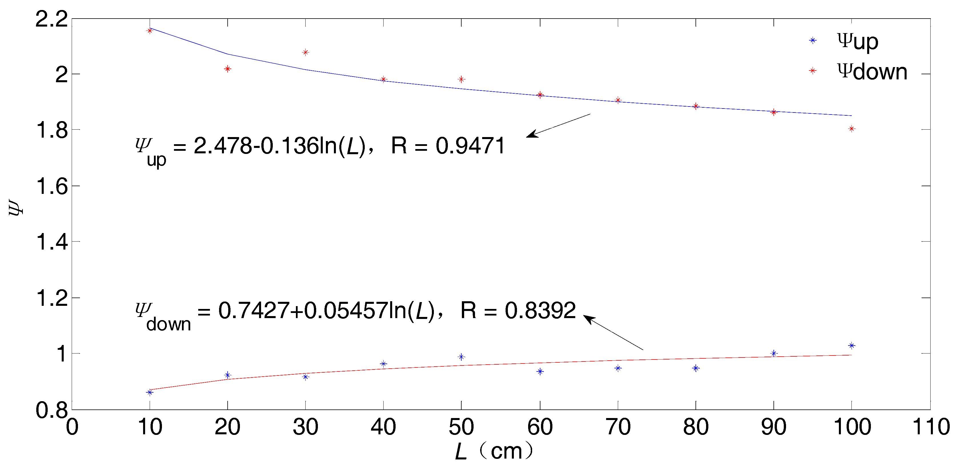
Based on the NN anisotropic parameter ψ, the interval ranges of the anisotropic parameters of all sizes are shown in Figure 3. Both the upper and lower bounds are fitted by the logarithmic curves, where the upper curve decreases and the lower curve increases as L increases.
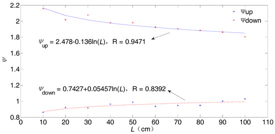
Figure 3.
The upper and lower bounds of the parameter ψ for different sized joint samples.
From Figure 3, we can obtain the NN anisotropic parameter ψ(L) corresponding to L for I ϵ [0, 0.5] as follows:
5. NN Functions for Reflecting the Scale Effect of Joint Surface Roughness
As we know, the roughness coefficient of a rock mass structure decreases with the increase of size, which is called the scale effect. In this section, we discuss this issue.
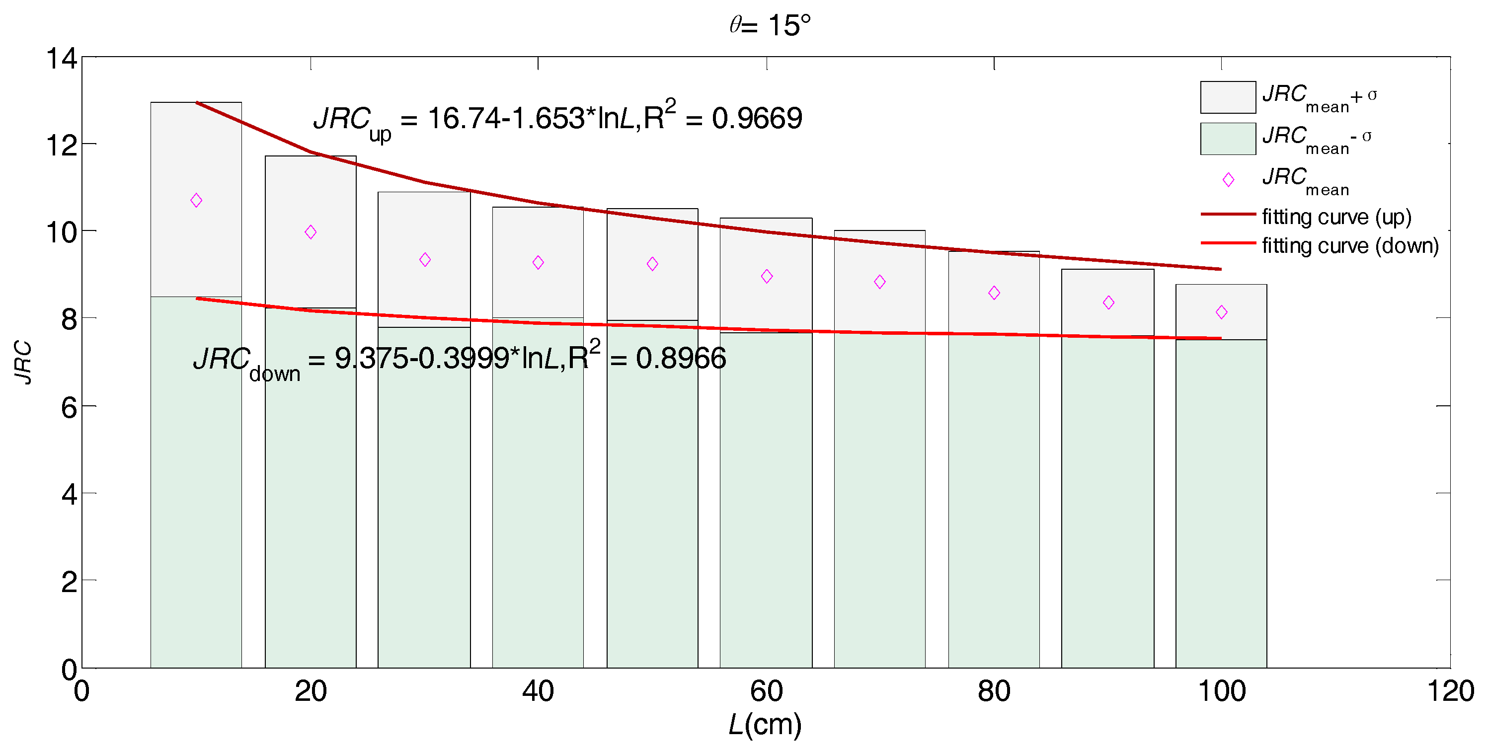
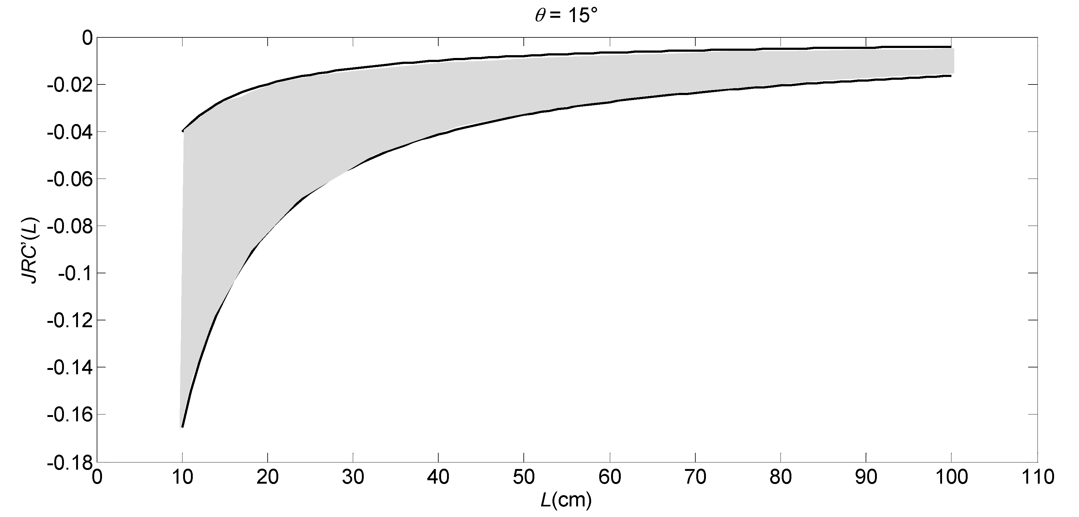
When the orientation is 15°, the JRC values on the increase of the joint sample sizes are shown in Figure 4, which apparently exhibit a negative scale effect. Then, the fitting curves present the logarithmic functions with monotonously-decreasing trends, and then both the upper and lower bounds are matched well.
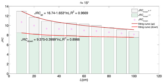
Figure 4.
JRC values of different sized joint samples in the orientation of 0°.
Thus, the NN function JRC(L) and its derivative function JRC’(L) for I ϵ [0, 0.5] are given as:
where a1 and a2 are the fitting parameters of the lower bounds and b1 and b2 are the twice of the difference of the lower and upper bounds. In the NN function JRC(L), a1 + a2lnL is the determinate part and (b1 + b2lnL)I is the indeterminate part.
For example, in Figure 4, a1 and a2 are 9.375 and −0.3999, respectively. Then, b1 and b2 can be obtained as follows:
According to Equations (10) and (11), we have the following results:
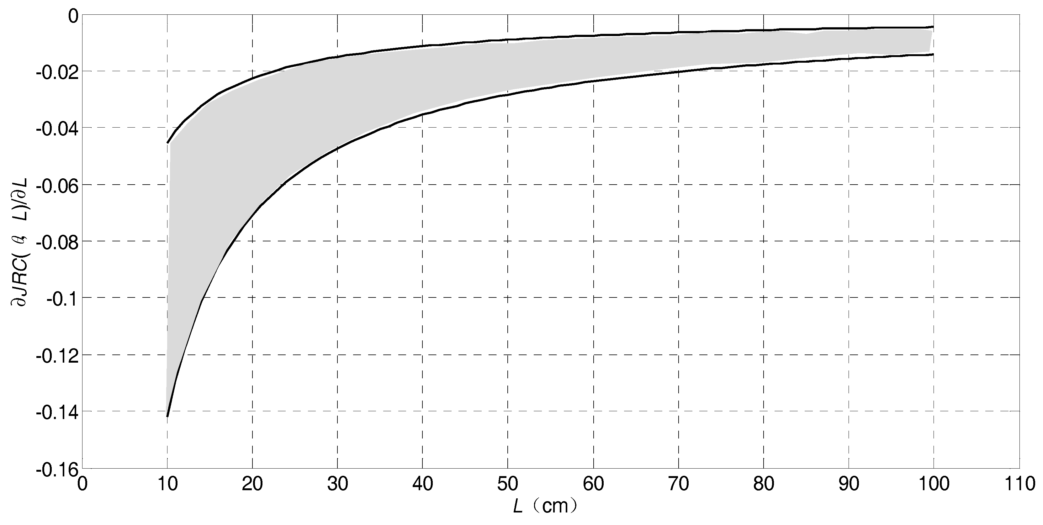
In Figure 5, the shaded part is the changing rate range of JRC’(L). It is monotonously increasing on the increase of L. Clearly, the scale effect phenomenon is more obvious in smaller sizes.

Figure 5.
The changing rates of upper and lower limits of JRC’(L) in various sizes.
By the similar method, fitting results of other orientations can also be obtained, the fitting parameters, NN functions for JRC(L), and derivative functions for JRC’(L) are tabulated in Table 3 and Table 4.

Table 3.
NN functions of JRC(L) for I ϵ [0, 0.5] corresponding to the JRC values of the joint samples in different orientations.

Table 4.
NN functions of JRC’(L) for I ϵ [0, 0.5] in different orientations.
6. NN Function of JRC with the Two Variables θ and L
As analyzed above, we have obtained the anisotropy and the scale effect of JRC, respectively, which are the important characteristics of the rock joint samples. In this section, we shall describe a NN function with the two variables θ and L, under NN environments.
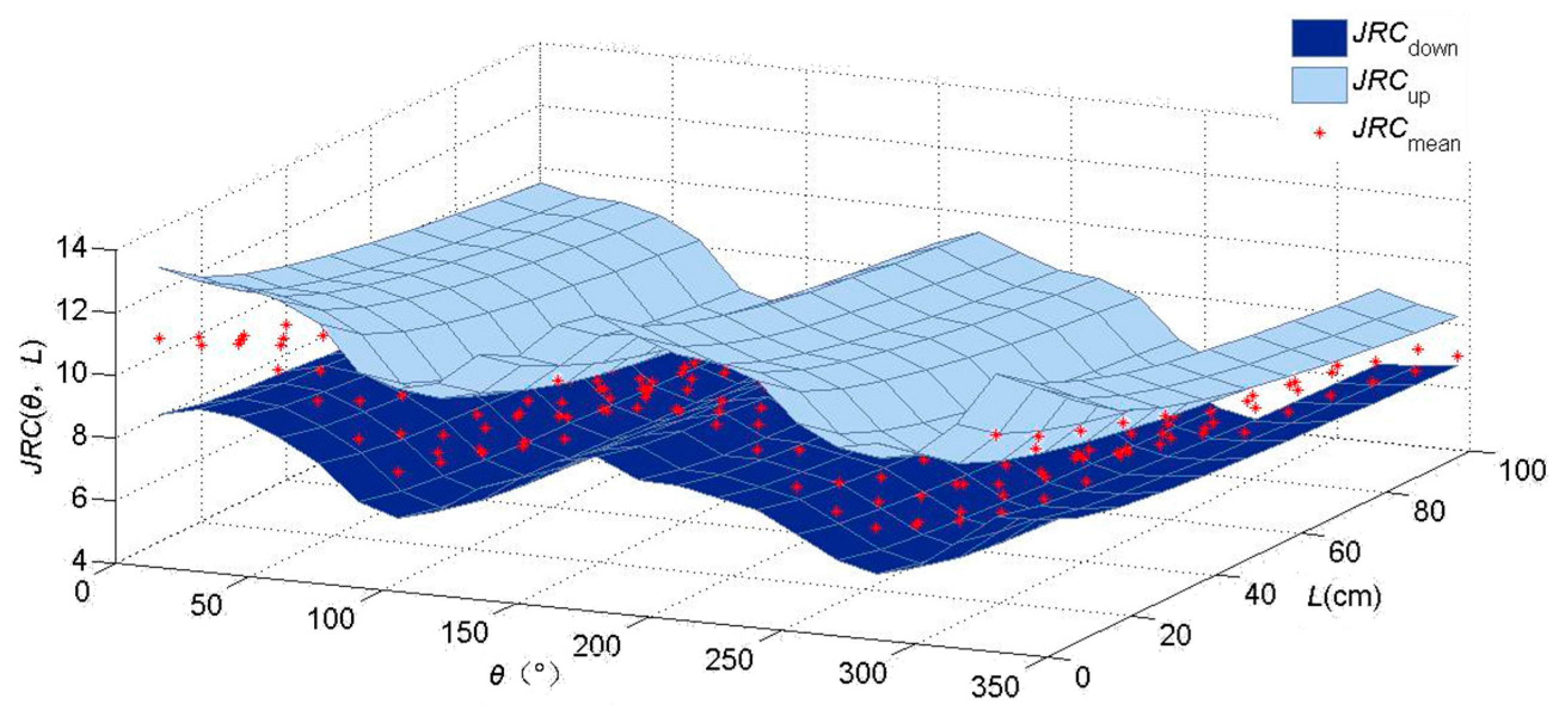
To find the relationship between the JRC values and the two variables θ and L, through numerical analyses, the trigonometric function polynomial of θ and L can fit into two smooth surfaces of the upper and lower bounds in the three-dimensional coordinate system, as shown in Figure 6. It is obvious that all of the points of mean values fall between the upper and lower surfaces. That is to say, the uncertain range almost contains all JRC values. Thus, the fitting equations based on the upper and lower surfaces of JRC values are presented as follows:
JRC(θ, L)down = −0.4536lnL + 1.382sinθ + 3.866sin2θ + 1.039cos3θ − 32.03sin4θ − 22.65sin5θ + 85.86sin6θ + 53.45sin7θ − 109.4sin8θ − 36.4sin9θ + 60.38sin10θ − 7.551cos11θ − 11.04sin12θ + 6.802cos13θ + 4.334sin15θ + 8.869,
JRC(θ, L)up = −1.42lnL + 2.08sinθ − 9.352sin2θ + 2.061cos3θ + 71.78sin4θ − 46.69sin5θ − 255.3sin6θ + 117.2sin7θ + 444.2sin8θ − 81.64sin9θ − 383.1sin10θ − 18.68cos11θ + 128.9sin12θ + 16.96cos13θ + 9.156sin15θ + 15.74.
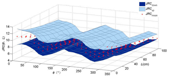
Figure 6.
Curved surface area of JRC values corresponding to both L and θ.
Then, the NN function JRC(θ, L) for I ϵ [0, 0.5] is given as follows:
JRC(θ, L) = (−0.4536 − 1.9328I)lnL + (1.382 + 1.396I)sinθ + (3.866 − 26.436I)sin2θ + (1.039 + 2.044I)cos3θ + (−32.03 + 207.62I)sin4θ + (−22.65 − 48.08I)sin5θ + (85.86 − 682.32I)sin6θ + (53.45 + 127.5I)sin7θ + (−109.4 + 1107.2I)sin8θ + (−36.4 − 90.48I)sin9θ + (60.38 − 886.96I)sin10θ + (−7.551 − 22.258I)cos11θ + (−11.04 + 279.88I)sin12θ + (6.802 + 20.316I)cos13θ + (4.334 + 9.644I)sin15θ + (8.869 + 13.742I), for I = [0, 0.5].
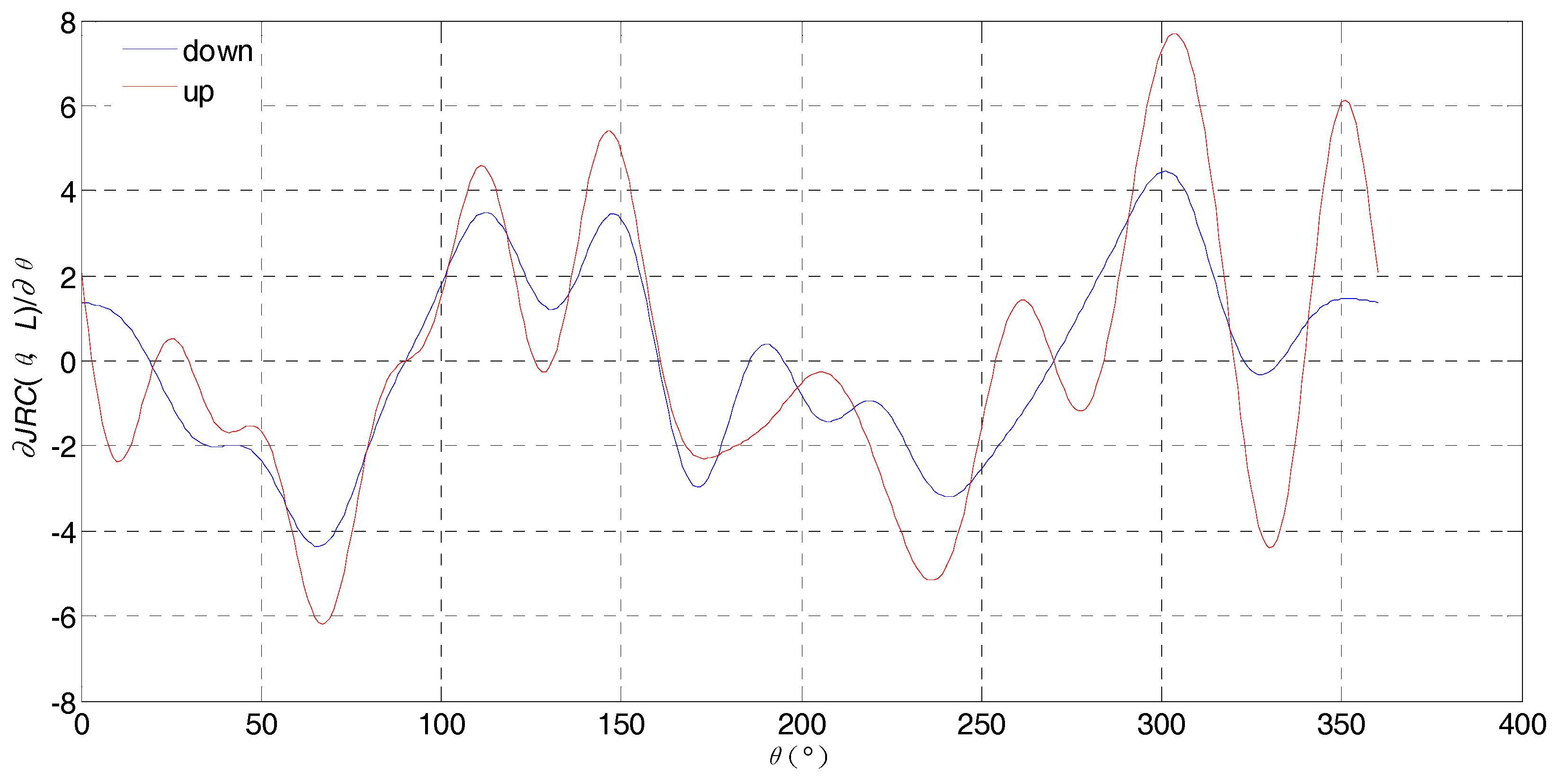
By the partial derivative of Equation (12), we can obtain the changing rate functions of the scale effect and the anisotropy:
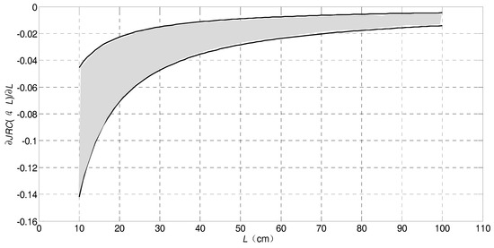
Figure 7.
The changing rates of the scale effect.
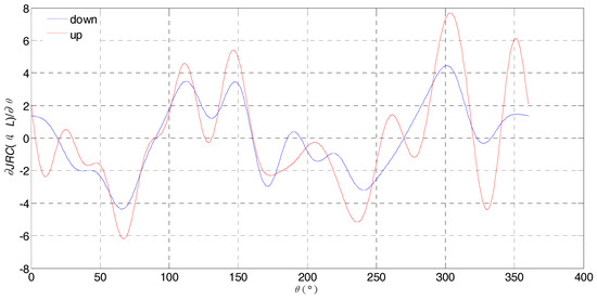
Figure 8.
The changing rates of the anisotropy.
7. Discussion
In this study, we investigated the anisotropy and scale effect of indeterminate JRC values by some unary NN functions and two-variable NN function, respectively, based on an actual case analysis. Generally speaking, the JRC characteristics reflected by the two-variable NN function are more comprehension and offer more details, effectively indicating the anisotropy and scale effect of indeterminate JRC values simultaneously, although the NN function itself is more complex.
Obviously, the proposed NN functions can not only express the JRC values with indeterminate information effectively and reasonably instead of the crisp values of JRC in the existing literature, but also indicates the anisotropy and scale effect of the indeterminate JRC values completely/simultaneously. However, the existing classical analysis methods cannot express and deal with such types of indeterminate JRC values and may lose much more information. Then, the main advantage of NN functions is that the NN functions of JRC can express and deal with the indeterminate JRC values instead of the crisp JRC values and contain much more useful information under indeterminate (imprecise, unsure, and even completely unknown) environments. Hence, we use a NN function instead of any classical function/crisp function of JRC to express the indeterminate function of JRC because any NN function can approximate the average value function/crisp function of JRC. When there is no indeterminacy in the NN function, the NN function is degenerated to the crisp function. Since, in the real world, we cannot always compute or provide exact/crisp values for the JRC characteristics, we can at least approximate them by NN functions. However, any NN function can contain and approximate the average value function/crisp function in existing classical methods. Obviously, the NN function provides one effective way for passing from the classical crisp functions to the NN functions in analyzing the anisotropy and scale effect of JRC under indeterminate environments.
8. Conclusions
Based on the concept and operations of NNs, the two NN functions JRC(θ) and JRC(L) were developed for the first time to express the anisotropy and the scale effect of indeterminate JRC values, respectively. To indicate the anisotropic characteristic of JRC, the NN parameter ψ was defined to quantify the anisotropic degree. Additionally, the derivative functions JRC’(θ) and JRC’(L) were utilized to describe their changing rates in various measurement orientations and sample sizes. Finally, a two-variables NN function JRC(θ, L) was presented to express the indeterminate information of JRC values in the sample sizes and measurement orientations and to investigate the changing rates by its partial derivative functions. It is obvious that the NN functions can effectively express the uncertainties of JRC and provide a new effective way for the JRC expression and analysis under indeterminate environments. In future work, we have to extend the NN function to the shear strength expression and conduct analyses under indeterminate environments.
Acknowledgments
This paper was supported by the National Natural Science Foundation of China (No. 71471172).
Author Contributions
Jun Ye proposed the expression and analysis methods of JRC using NN functions; Jiquan Chen and Rui Yong provided the NN functions and analyses of indeterminate JRC values; Shigui Du gave the measurement data and statistical analysis of JRC; and we wrote the paper together.
Conflicts of Interest
The authors declare that we have no conflict of interest regarding the publication of this paper.
References
- Barton, N.; Choubey, V. The shear strength of rock joints in theory and practice. Rock Mech. 1977, 10, 1–54. [Google Scholar] [CrossRef]
- Chen, S.J.; Zhu, W.C.; Liu, S.X. Anisotropy and size effects of surface roughness of rock joints. J. Eng. Geol. 2015, 34, 57–66. (In Chinese) [Google Scholar]
- Alameda-Hernández, P.; Jiménez-Perálvarez, J.; Palenzuela, J.A.; Hamdouni, R.E.; Irigaray, C.; Cabrerizo, M.A.; Chacón, J. Improvement of the JRC calculation using different parameters obtained through a new survey method applied to rock discontinuities. Rock Mech. Rock Eng. 2014, 47, 2047–2060. [Google Scholar] [CrossRef]
- Jang, H.S.; Kang, S.S.; Jang, B.A. Determination of joint roughness coefficients using roughness parameters. Rock Mech. Rock Eng. 2014, 47, 2061–2073. [Google Scholar] [CrossRef]
- Grasselli, G.; Wirth, J.; Egger, P. Quantitative three-dimensional description of a rough surface and parameter evolution with shearing. Int. J. Rock Mech. Min. Sci. 2002, 39, 789–800. [Google Scholar] [CrossRef]
- Lee, Y.H.; Carr, J.R.; Barr, D.J.; Haas, C.J. The fractal dimension as a measure of the roughness of rock discontinuity profiles. Int. J. Rock Mech. Min. Sci. 1990, 27, 453–464. [Google Scholar] [CrossRef]
- Li, Y.; Huang, R. Relationship between joint roughness coefficient and fractal dimension of rock fracture surfaces. Int. J. Rock Mech. Min. Sci. 2015, 75, 15–22. [Google Scholar] [CrossRef]
- Li, H.; Huang, R. Method of quantitative determination of joint roughness coefficient. J. Eng. Geol. 2014, 33 (Suppl. S2), 2513–2519. (In Chinese) [Google Scholar]
- Sun, F.; She, C.; Wan, L. Research on a new roughness index of rock joint. J. Eng. Geol. 2013, 33, 3489–3497. (In Chinese) [Google Scholar]
- Aydan, O.; Shimizu, Y.; Kawamoto, T. The anisotropy of surface morphology characteristics of rock discontinuities. Rock Mech. Rock Eng. 1996, 29, 47–59. [Google Scholar] [CrossRef]
- Barton, N. Review of a new shear-strength criterion for rock joints. Eng. Geol. 1973, 7, 287–332. [Google Scholar] [CrossRef]
- Barton, N.; Bandies, S. Review of predictive capabilities of JRC-JCS model in engineering practice. Proc. Int. Symp. Rock Jt. 1991, 181, 603–610. (In Chinese) [Google Scholar]
- Du, S.G.; Hang, M.; Luo, Z.Y.; Jia, R.D.; Wang, Y.M. Scale effect of undulation amplitude of rock joints. J. Eng. Geol. 2010, 18, 47–52. (In Chinese) [Google Scholar]
- Chen, S.J.; Zhu, W.C.; Yu, Q.L.; Liu, X.G. Characterization of anisotropy of joint surface roughness and aperture by variogram approach based on digital image processing technique. Rock Mech. Rock Eng. 2016, 49, 855–876. [Google Scholar] [CrossRef]
- Ye, J.; Yong, R.; Liang, Q.F.; Huang, M.; Du, S.G. Neutrosophic functions of the joint roughness coefficient and the shear strength: A case study from the pyroclastic rock mass in Shaoxing City, China. Math. Probl. Eng. 2016, 2016, 4825709. [Google Scholar] [CrossRef]
- Smarandache, F. Neutrosophy: Neutrosophic Probability, Set, and Logic; American Research Press: Rehoboth, DE, USA, 1998. [Google Scholar]
- Smarandache, F. Introduction to Neutrosophic Measure, Neutrosophic Integral, and Neutrosophic Probability; Sitech & Education Publisher: Craiova, Romania, 2013. [Google Scholar]
- Smarandache, F. Introduction to Neutrosophic Statistics; Sitech & Education Publisher: Craiova, Romania, 2014. [Google Scholar]
- Ye, J. Multiple-attribute group decision-making method under a neutrosophic number environment. J. Intell. Syst. 2016, 25, 377–386. [Google Scholar] [CrossRef]
- Ye, J. Bidirectional projection method for multiple attribute group decision making with neutrosophic numbers. Neural Comput. Appl. 2017, 28, 1021–1029. [Google Scholar] [CrossRef]
- Kong, L.W.; Wu, Y.F.; Ye, J. Misfire fault diagnosis method of gasoline engines using the cosine similarity measure of neutrosophic numbers. Neutrosophic Sets Syst. 2015, 8, 43–46. [Google Scholar]
- Ye, J. Fault diagnoses of steam turbine using the exponential similarity measure of neutrosophic numbers. J. Intell. Syst. 2016, 30, 1927–1934. [Google Scholar] [CrossRef]
- Chen, J.Q.; Ye, J. A projection model of neutrosophic numbers for multiple attribute decision making of clay-brick selection. Neutrosophic Sets Syst. 2016, 12, 139–142. [Google Scholar]
- Liu, P.; Liu, X. The neutrosophic number generalized weighted power averaging operator and its application in multiple attribute group decision making. Int. J. Mach. Learn. Cybern. 2016, 1–12. [Google Scholar] [CrossRef]
- Ye, J. Neutrosophic number linear programming method and its application under neutrosophic number environments. Soft Comput. 2017. [Google Scholar] [CrossRef]
- Du, S.G. A simple longitudinal profiler and its application in the study of roughness coefficient of rock mass structural plane. Geol. Sci. Technol. Inf. 1992, 11, 91–94. [Google Scholar]
- Zhang, G.C.; Karakus, M.; Tang, H.M.; Ge, Y.F.; Zhang, L. A new method estimating the 2D loint roughness coefficient for discontinuity surfaces in rock masses. Int. J. Rock Mech. Min. Sci. 2014, 72, 191–198. [Google Scholar]
- Tatone, B.S. Quantitative Characterization of Natural Rock Discontinuity Roughness In-Situ and in the Laboratory. Master’s Thesis, University of Toronto, Toronto, ON, Canada, 2009. [Google Scholar]
© 2017 by the authors. Licensee MDPI, Basel, Switzerland. This article is an open access article distributed under the terms and conditions of the Creative Commons Attribution (CC BY) license (http://creativecommons.org/licenses/by/4.0/).

