Article

Correction of Outliers in Temperature Time Series Based on Sliding Window Prediction in Meteorological Sensor Network

1
School of Computer and Software, Nanjing University of Information Science & Technology, Nanjing 210044, China
2
Jiangsu Collaborative Innovation Center on Atmospheric Environment and Equipment Technology, Nanjing 210044, China
3
Jiangsu Engineering Center of Network Monitoring, Nanjing University of Information Science & Technology, Nanjing 210044, China
*
Authors to whom correspondence should be addressed.
Information 2017, 8(2), 60; https://doi.org/10.3390/info8020060
Submission received: 28 March 2017 / Revised: 17 May 2017 / Accepted: 19 May 2017 / Published: 24 May 2017

Abstract

:
In order to detect outliers in temperature time series data for improving data quality and decision-making quality related to design and operation, we proposed an algorithm based on sliding window prediction. Firstly, the time series are segmented based on the sliding window. Then, the prediction model is established based on the history data to predict the future value. If the difference between a predicted value and a measured value is larger than the preset threshold value, the sequence point will be judged to be an outlier and then corrected. In this paper, the sliding window and parameter settings of the algorithm are discussed and the algorithm is verified on actual data. This method does not need to pre classify the abnormal points and perform fast, and can handle large scale data. The experimental results show that the proposed algorithm can not only effectively detect outliers in the time series of meteorological data but also improves the correction efficiency notoriously.

1. Introduction

Meteorological observation is the basis for the development of meteorology and atmospheric science. Meteorological observation data and meteorological information not only provide daily information for weather forecasts, but are also processed into important climate data for agriculture, forestry, industry, traffic, military, hydrology, health and environmental protection departments through long-term accumulation and statistics [1]. The meteorological disaster monitoring network using atmospheric remote sensing and high-speed communication transmission technology can directly issue a tornado, strong storm and typhoon weather warning in a timely way to the users [2]. The observation of air temperature is an especially important item in the ground meteorological observation. Air temperature records can be used to characterize the thermal status of a place. It is indispensable whether in theoretical research or in the application of national defense and economic construction. Therefore, it is very important to ensure the accuracy of temperature observation.
The artificial observation gradually turns to the automatic observation, and the observation automation level is continuously improved. At present, China has built 2423 National Automatic Weather Stations (AWSs) [3,4]. The basic meteorological factors such as temperature, humidity, air pressure, wind speed, and wind direction have achieved automatic observation and the observation frequency is up to the minute level. Towards the end of 2012, the number of China’s AWSs has reached 46,000. However, the average distance of AWS is only about 20 km. For densely populated China, this coverage is far from enough. For modern weather forecasts, it is necessary to have enough accurate weather information for improving decision-making quality related to design and operation.
The unique characteristics of wireless sensor networks (WSN) [5,6] have been favored by the scientific community and the military. It has been widely used in many fields, such as battlefield monitoring [7], environmental protection [8] , industrial control [9] and so on. The meteorological sensor network is defined as a network composed of meteorological sensor nodes, sink nodes, wireless communication facilities, and so on [10]. It can monitor and collect many kinds of weather information, such as temperature, humidity, air pressure, and wind speed. The obtained information will be processed and transmitted by a wireless multi hop mode, and finally sent to the control center by the sink nodes. Loading cheap weather sensors on nodes in meteorological sensor networks can greatly reduce the cost of meteorological data monitoring. In addition, as a a low cost temperature sensor, SHT15 (a kink of intelligent chip) is embedded in our sensing nodes for both air relative humidity and temperature sensing, which successfully reduces the cost of the specialized temperature sensor HMP45D from over $500 to $5. Thus, it can be deployed in a large area to improve the monitoring density. Thus, we have deployed this sensor in the playground, roof, observation stations and other places of our university for data collection.
However, low cost meteorological sensors are vulnerable to external factors. This often leads to some errors between the measured data and the standard data because of its unstable performance. In order to improve the accuracy and practicability of the meteorological sensor network, it is necessary to establish a modified model to correct the measured data. According to the temperature data measured by the temperature and humidity sensor SHT15 [11] in the meteorological sensor network, some researchers in paper [12] have found the reasons for affecting the quality of the data. In addition, they have put forward a corresponding correction model. They used the solar radiation intensity as the auxiliary parameter and established the relationship between the errors and the values of solar radiation. Thus, the corresponding relation table of error and solar radiation was established. Then, the temperature data was corrected by using a look-up table. Figure 1 shows the result of node data correction in paper [12]. We can see that the model can correct most errors of the measured values, but it can not correct the outliers in the data, so it will lead to a higher volatility. Therefore, we urgently need to deal with these outliers to reduce volatility.
For the small size of the data set, the data administrator can directly use a simple chart or manually to detect and deal with outliers. However, for massive datasets or data streams, we need to use machines to detect and deal with outliers automatically and efficiently.
As one of the challenging problems in the field of data mining [13], time series mining [14] has been widely used in the field of hydrological time series similarity search [15], sequential pattern mining and cycle analysis [16,17]. This paper presents an algorithm for outlier detection of temperature time series based on sliding window prediction in the meteorological sensor network. The proposed algorithm can predict the future data by the sliding window method. In addition, the difference between the predicted value and the measured value is calculated to determine whether it is an outlier. If the difference between the predicted value and the measured value is larger than the preset threshold value, the sequence point will be judged as an outlier and then corrected. The experimental results show that the method can effectively correct the outliers in a temperature time series. Thus, it can achieve the purpose of improving the temperature time series analysis in the meteorological sensor network.
This paper is organized as follows. In Section 2, we describe the related work of time series outlier detection and error correction in the meteorological sensor network. In Section 3, we demonstrate the process of temperature time series outlier detection and correction. In Section 4, we present the experiment foundation and experimental results and analysis. Finally, Section 5 presents the conclusions.

2. Related Work

2.1. Error Correction in Meteorological Sensor Networks

Existing work on an error correction model in a meteorological wireless sensor network can be divided into two categories: Statistic Based and Back Propagation Neural Network (BP) Based.
Statistic based: A statistic based error correction model in meteorological wireless sensor network leverage statistical methods to establish the relationship between solar radiation (SR) and errors. In paper [12], they analysed all of the collected data of air temperature (AT) and SR in May 2014 and found the numerical correspondence between them. This corresponding relation was used to calculate real-time error corresponding to SR and correct the error of AT in other months. Although this method can reduce a lot of errors, there are also many outliers in the time series. On the basis of their work, we continued to carry out the outlier correction.
BP based: In order to solve the problem of the big fluctuation caused by statistics based error correction system in paper [12], paper [18] leverage BP neural network to establish the relationship between SR and error. The BP neural network is one of the most widely used neural network models. It can learn and store a large amount of input–output models’ mapping relationship. They use a BP neural network to do nonlinear regression to establish the association between AT and SR. It proves that the BP neural network is very suitable for solving this problem due to its powerful functions of nonlinear fitting. However, they still can not solve the problem of too much volatility in corrected data perfectly.

2.2. Outlier Detection

An outlier can be defined as an observation that deviates so much from other observations as to arouse suspicion that it was generated by a different mechanism [19], or patterns in data that do not conform to a well-defined notion of normal behav [20]. Outlier detection is also called outlier mining or anomaly detection. This is a process of extracting hidden information that people do not know in advance but is potentially useful from a large number of data. The major objective of outlier detection is to identify data objects that are markedly different from, or inconsistent with, the remaining set of data [21]. Outlier detection needs to solve two main problems: define what kind of data is abnormal in a given data set; and find an effective way to detect such abnormal data.
According to the different forms of the outliers in the time series, the time series outlier detection can be divided into three types: sequence anomalies, point anomalies and pattern anomalies. At present, time series anomaly detection methods mainly include the following:
(1)
Window based method [22,23]. The time series is divided into several fixed size series (window), and then locate the outliers in each series. The method is based on the fact that the outliers in time series may be caused by outliers in one or more series.
(2)
Distance based method [24,25]. In this method, the feature points are used to represent the series. Then, using the two order regression model to realize the unequal division of series. Based on the dynamic time warping distance, the abnormal scores of subsequence are calculated. Then, select the largest k values of the abnormal score to determine whether it is an outlier.
(3)
Density based method [26,27]. This method does not use Yes or No to determine whether a point is an outlier, but uses a weight to evaluate its degree of outlier. This is a local detection algorithm, which means that the degree depends on the isolation of the object relative to its neighborhood.
(4)
Support Vector Machine (SVM) based method [28,29]. In this method, the support vector regression is used to establish the regression model of the historical time series. Then, the matching degree between the new series and the model is judged. In addition, One-Class SVM technology has been widely used in the field of outlier detection.
(5)
Clustering based method [30,31]. The method first divides the data set into several clusters, and the data points that do not belong to any cluster are outliers. In the field of anomaly detection, clustering technology is used for unsupervised detection and semi-supervised detection. However, anomaly detection is usually a by-product of the clustering algorithm.
To sum up, the performance of the window based method depends on the width of the window. If the width of the window is too large or too small, the accuracy of the test results will be both affected. Distance based method has high time complexity. The clustering based method depends on the number of clusters and the existence of outliers in the data. The authors of Reference [32] think that outlier detection based on time series forecasting is the most simple and intuitive method, but the predictive ability of this method depends on the prediction model, and it is difficult to determine a reasonable threshold.
Faced with such challenges, we proposed a method to detect outliers that splits given historical temperature time series into subsequences by a sliding-window. An autoregressive (AR) prediction model [33] was used to predict the value of the next point and prediction confidence interval (PCI) was calculated from nearest-neighbor historical data. If the predicted value falls outside the PCI, it will be judged to be an outlier. The AR prediction model belongs to the data-driven time series model essentially. Thus, it is simpler to develop and can rapidly produce accurate short forecast horizon predictions. There are two reasons for this paper to use PCI to judge the outliers. Firstly, the correlations between adjacent data points in time series are certainly higher than those farther away points. Secondly, the PCI can be calculated dynamically according to different nearest-neighbor windows size and confidence coefficient of difference users, which make it suitable for different variables of meteorological time series outlier detection for different users’ demand.

3. Time Series Outlier Detection Based on Sliding Window Prediction

3.1. Relevant Definition

A time series is a set of data points indexed (or listed or graphed) in time order. The temperature time series is a time-varying phenomenon that records the temperature data changes according to time.
Definition 1.
Temperature time series D n is an ordered collection of elements composed of record values and record time. D n = { d 1 = ( v 1 , t 1 ) , d 2 = ( v 2 , t 2 ) , . . . , d n = ( v n , t n ) } , where point d i = ( v i , t i ) represents the observed value v i at the time t i .
The first problem to be solved in the anomaly detection of temperature time series is to define what kind of data is abnormal in the given data set. The definition of outlier determines the goal of outlier mining. In general, the change in the value of temperature is relatively modest. In addition, because of some unexpected situations, the temperature will change rapidly. However, from an empirical point of view, abnormal data are often produced in large fluctuations.
Definition 2.
Abnormal temperature time series. Given a set of temperature time series D n = { d 1 = ( v 1 , t 1 ) , d 2 = ( v 2 , t 2 ) , . . . , d n = ( v n , t n ) } , where point d i = ( v i , t i ) represents the observed node temperature data v i of the time t i . Use η i ( k ) = d i 2 k , d i 2 k + 1 , , d i 1 to express the k-nearest neighbor window of point d i . The observed value set is denoted as v i 2 k , v i 2 k + 1 , , v i 1 . If the difference between the actual observation point d i and the predicted value of k-nearest neighbor window model exceed a specific threshold τ, the point will be identified as an outlier. According to the above definition, the k-nearest neighbor window and the threshold τ becomes the basis for judging whether d i is an outlier.

3.2. Algorithm Description

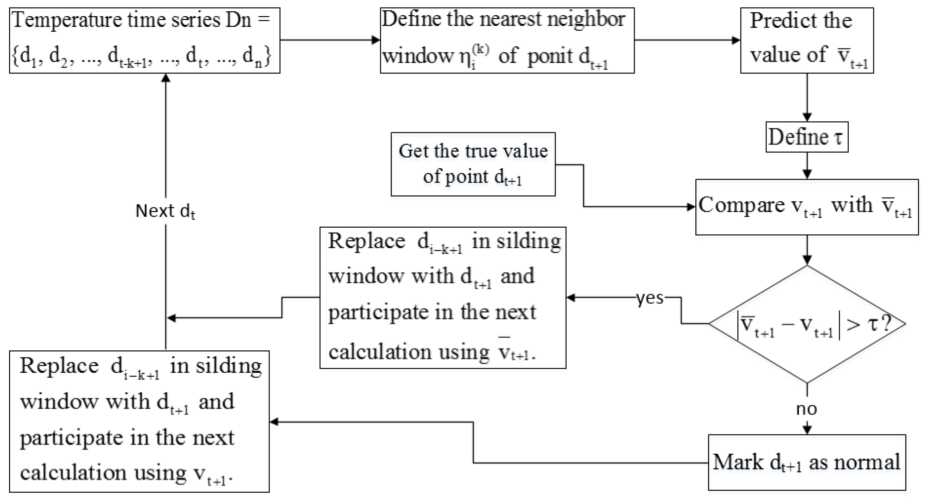
In this paper, the core ideas of the outlier detection method based on sliding window are as follows: define the k-nearest neighbor window η i ( k ) of point d i according to different application requirements. Establish a one-step-ahead prediction model and use the observation set of η i ( k ) as an input parameter to predict the observed value v i of point d i ; and calculate the confidence interval ( v i ± τ ) of d i corresponding to the predicted value v i , where the threshold can be calculated by the confidence level p and the window width k. When the actual value v i of point d i was obtained, a comparison was made between the predicted values of v i and v i . If v i outside of ( v i ± τ ), then the point d i will be judged as an outlier. Move the sliding window backward and use d i replace d i 2 k and update η i ( k ) . Then, determine the next node until all nodes are detected. The overall flow of the algorithm is shown in Figure 2.

3.2.1. Sliding Window Definition

The first step of outlier detection algorithm in time series D n is defining the sliding neighbor window of point d i . In order to reduce the computational complexity of the algorithm, it is only necessary to use the k-nearest neighbor node of d i as the input parameters of the prediction model. A neighbor node window can be divided into two types: unilateral and bilateral. Bilateral neighbor node window is suitable for the condition of both the predecessor and the subsequent window data of the node are known. A unilateral neighbor node window contains only the precursor data of the node.
The anomaly detection algorithm based on prediction only needs to select the left neighbor window of a data point to determine whether this data point is outlier or not. A unilateral k-neighbor window η i ( k ) can be defined as follows:
η i ( k ) = d i 2 k , d i 2 k + 1 , , d i 1 ,
where 2k is the size of the neighborhood window ranging from i 2 k to i 1 .

3.2.2. Prediction Model

The core of the outlier detection algorithm based on prediction is to build a one-step-ahead prediction model. The sliding window is used as the input parameter to predict the value of the subsequent node. A sliding window η i ( k ) = { d 1 , d 2 , . . . , d i } is used as the input parameter of the one-step-ahead time series prediction model to predict the observed values of d i , and the prediction algorithm can be formally expressed as:
d i + 1 = M ( η i ( k ) ) ,
where M() is an autoregressive ( A R ) prediction model. It is a statistical method to deal with the time series, which uses the historical performance of variables to predict the future performance of the variables, and assumes that they are linear. The advantage of the autoregressive method is that it does not require much information. The A R model forecasts future measurements in time series datasets, that is, η i ( k ) , from the same discharge site; they are used because they avoid complications caused by different sampling frequencies that can arise if a heterogeneous set of time series data was used.
The premise of the anomaly detection algorithm is based on the assumption that the observed values of k + 1 moments can be described by k finite precursor measurements. The implicit assumption is that the time series is a k order Markov process. Reference [32] compares the simple prediction model, the nearest neighbor prediction model, the single layer linear network prediction model and the multi-layer perceptron model on different datasets and concludes that the single-layer linear network prediction model can get better detection results than other models. Based on their work, the single layer linear network is used as the prediction model in this paper. It is assumed that the observed value of the t moment is a linear combination of its predecessor adjacency window:
v i ¯ = ( i = 1 2 k ( w t i v t i ) ) / ( i 1 2 k w t i ) ,
where w t 2 k , w t 2 k + 1 , . . . , w t 1 represent the weight vectors of the neighbor window nodes. The closer the distance between nodes is, the greater the weight is. In order to simplify the calculation, the weight vector { w t 2 k , w t 2 k + 1 , . . . , w t 1 } was assigned to { 1 , 2 , . . . , 2 k } .

3.2.3. Outlier Determination and Correction

Using the neighbor window of the tested point as the input parameter, calculate the predicted value and the confidence interval. The confidence interval gives the possible values of the predicted values. The confidence coefficient indicates that the expected frequency of the actual measured values fall within this range. If the model residuals are assumed to have zero-mean Gauss distribution, the p % PCI can be calculated as follows:
τ = t α / 2 , 2 k 1 × s 1 + 1 / ( 2 k ) ,
P C I = v i + 1 ^ ± τ ,
where v i + 1 ^ is the predicted value calculated by the prediction model according to the test point. t α / 2 , 2 k 1 is the percentile of the degrees of freedom for 2 k 1 t-distribution. s is the standard deviation of the model residuals. k is the size of the sliding window. If the actual observation value falls within the confidence interval, the test point is marked as a normal point; otherwise, it is classified as an outlier. Then, the predicted value is used to replace the abnormal value and is involved in the next round. As a threshold to determine whether a node is an outlier, PCI can effectively adjust the width of the window, so as to avoid the probability of false detection caused by the threshold selection.

3.3. Parameter Selection

In order to detect the outliers in time series, the abnormal point prediction method based on a sliding window needs to calculate the reasonable threshold of test points. Hence, the values of two parameters involved in the algorithm, k and p, become the key issues to improve the methods. Therefore, the following experimental method is used to select the appropriate parameters:
(1)
Window width k. k determines the number of neighboring points involved in the prediction. The larger the k value is, the more adjacent points are involved in the computation, and the computational complexity is increased accordingly. In order to select the optimal sliding window width, it varies k from 3 to 15 with an increment of 1, i.e., k = { 3 , 4 , . . . , 15 } .
(2)
Confidence coefficient p. It defines the expected probability that the measured values fall within the confidence interval. The greater the confidence coefficient is, the larger the range of confidence interval is. It varies the p range from 80% to 100% with an increment of 2%, i.e., p = { 80 % , 82 % , . . . , 100 % } .
The goal of outlier detection is to detect the outliers in time series as much as possible. Therefore, the criterion of the value of parameters ( k , p ) is to make the node data as close as possible to the standard temperature data collected by AWS in our university.

4. Experimental Analysis

In order to verify the validity of the temperature time series outlier detection method proposed in this paper, we use the real data to carry out the experiment and analyze the results of the algorithm.

4.1. Data Preparation

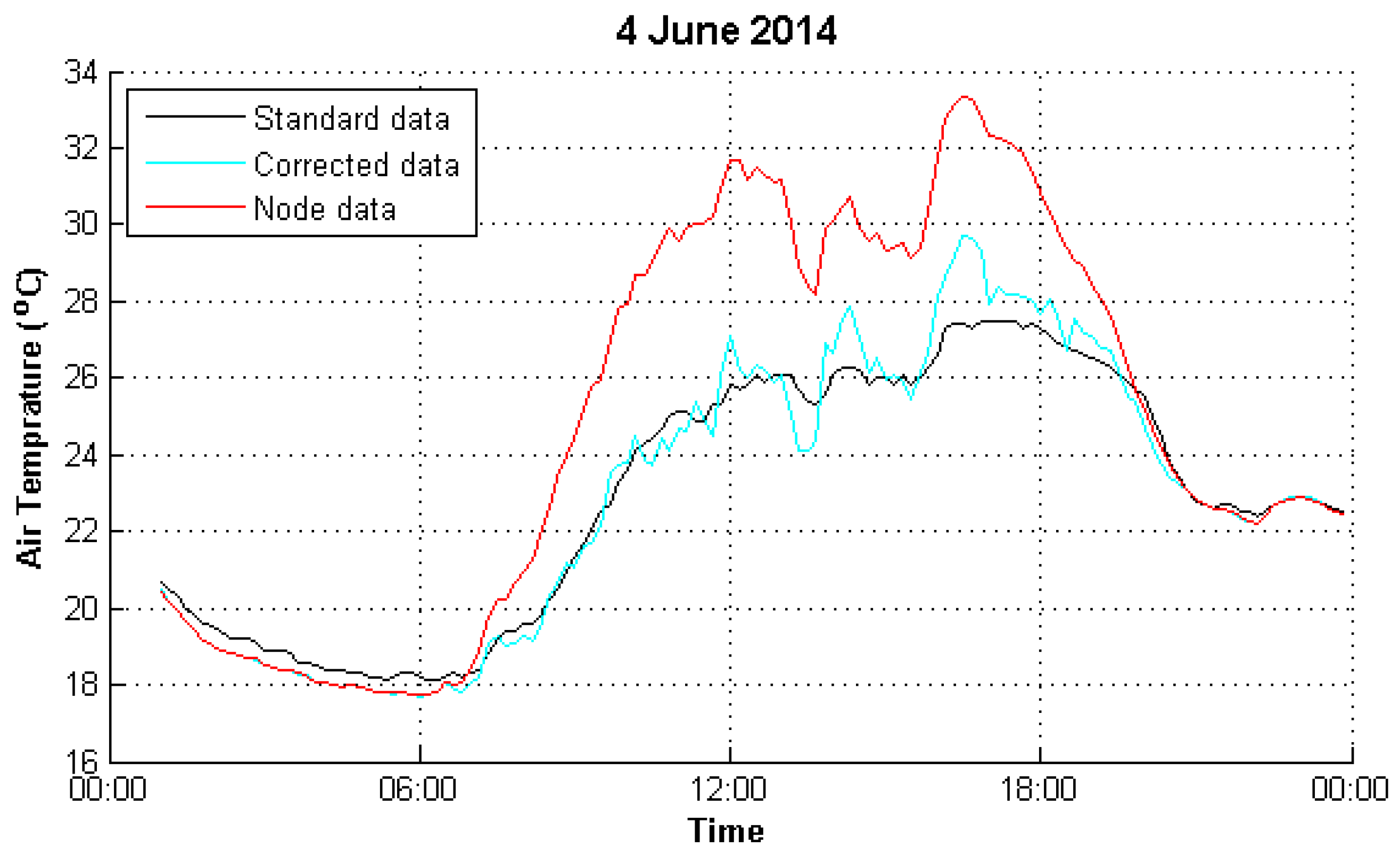
The data used in this paper consists of two parts. The first part is the standard temperature data collected from the standard automatic weather station (Serial number 59606) of Nanjing University of Information Science and Technology (NUIST). The other part is the node temperature data measured by the meteorological sensor network, which was built by ourselves. In this paper, the temperature data of a meteorological sensor network have been tentatively modified by the authors in [12]. Therefore, in this paper, based on the revised temperature data, we make a further correction. In order to illustrate the key problems in this paper, we select one of the representative data graphs from the data set. Figure 3 shows the temperature data for the whole day of 4 June 2014, the red line represents the original data measured by the sensor node, the blue line represents the revised node temperature in paper [12] and the black line is the standard temperature data. As we can see from Figure 3, after the correction scheme in the paper [12], the majority of the data error can be corrected, but the revised node data are still very volatile. The overall trend of the standard temperature curve is smooth, while some points in the node data deviate significantly from the neighbor points. These points can be regarded as outliers and should be processed further.

4.2. Result Evaluation

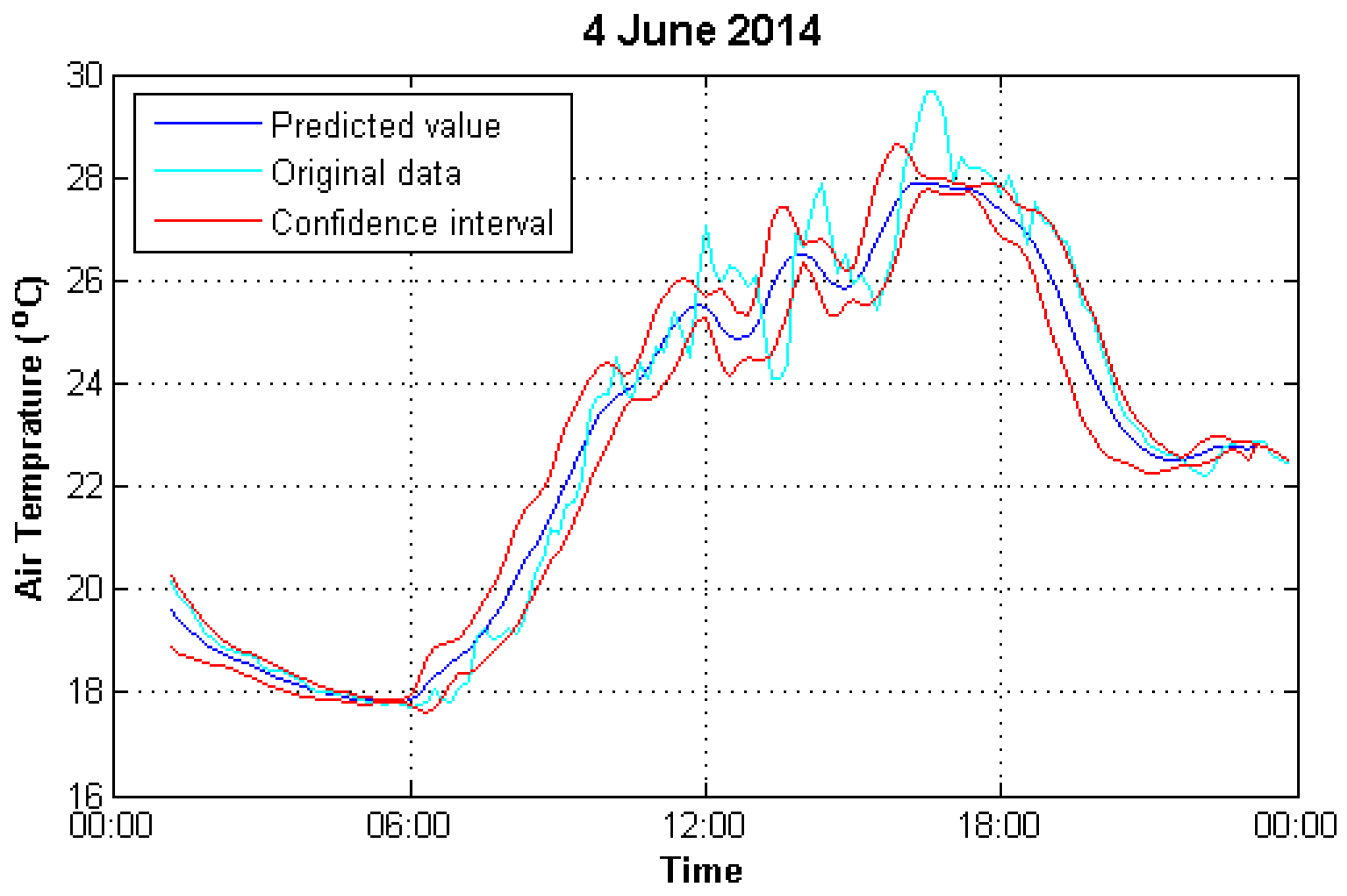
The standard data used in this experiment are derived from the standard automatic weather station at NUIST. This weather station was founded according to the AWS construction technical standard. It uses the HMP45D temperature and humidity sensors to collect temperature data and record a temperature data every minute. Then, the data is stored on the computer hard disk. The dataset we used includes 1 May 2014 to 1 January 2015. The data quality can be considered to meet the needs of users. Thus, the corrected node temperature data will be compared with it to determine whether the performance of the algorithm is good or bad. After a number of experiments and using different combinations of parameters, the effect achieves the best when (k, p) = (5, 95%). Similarly, the temperature data on 4 June 2014 are taken as examples to illustrate the results shown in Figure 4.
Figure 4 shows the measured value, the predictive value, the confidence interval and the correction value of the outlier detection algorithm in the given temperature time series dataset with the sliding window width k = 5 and the confidence level p = 95%. As we can see from Figure 4, the node data are very close to the standard data most of the time, but there is also a small part of the node data outside its confidence interval. According to the algorithm, these points will be identified as outliers. Thus, these outliers will be replaced by the predicted value, and the predicted value will participate in the next round of sliding window calculations.
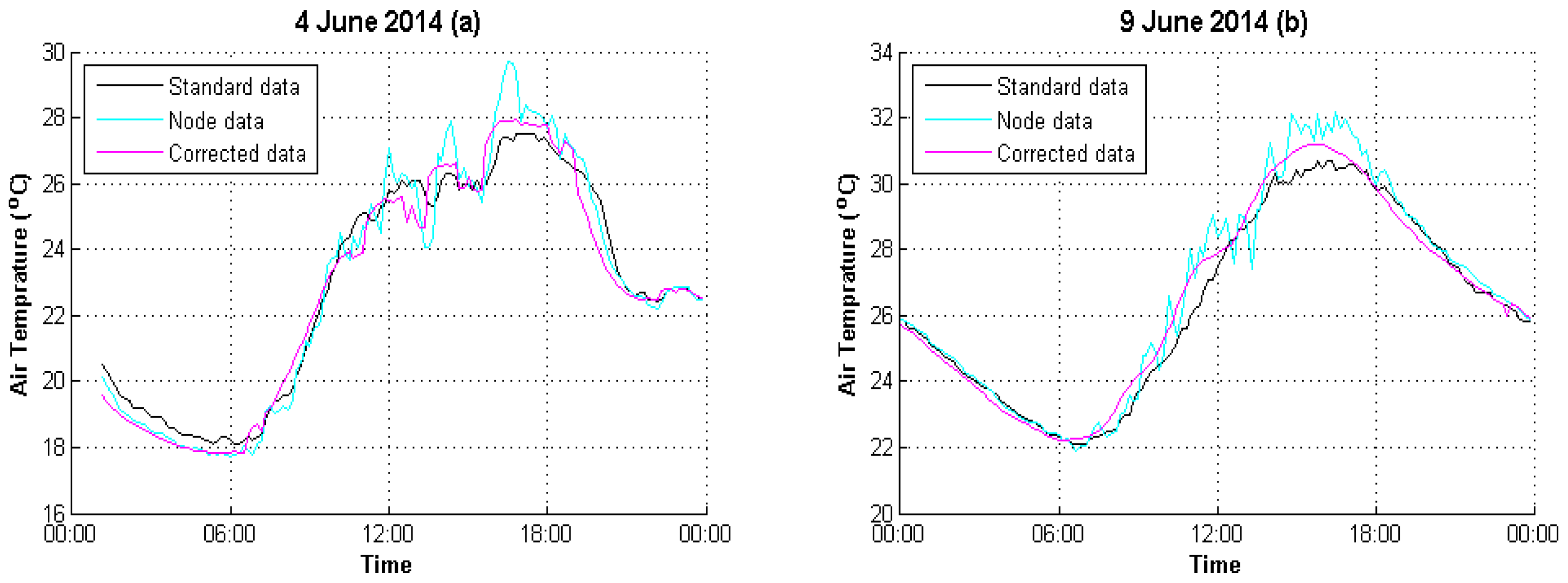
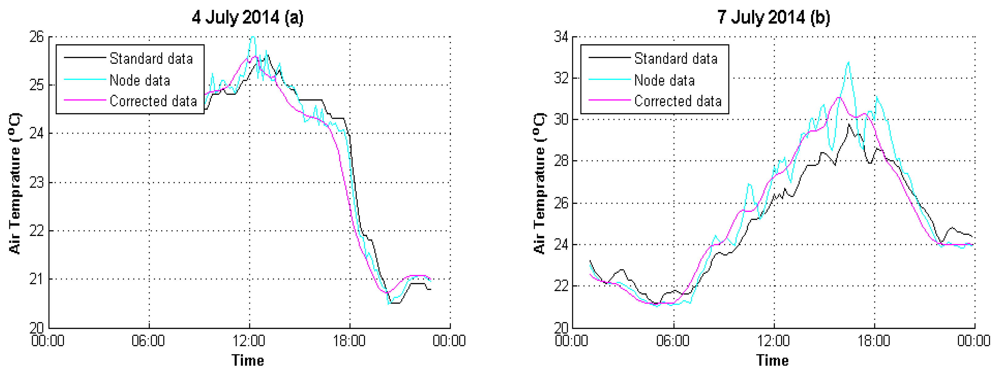
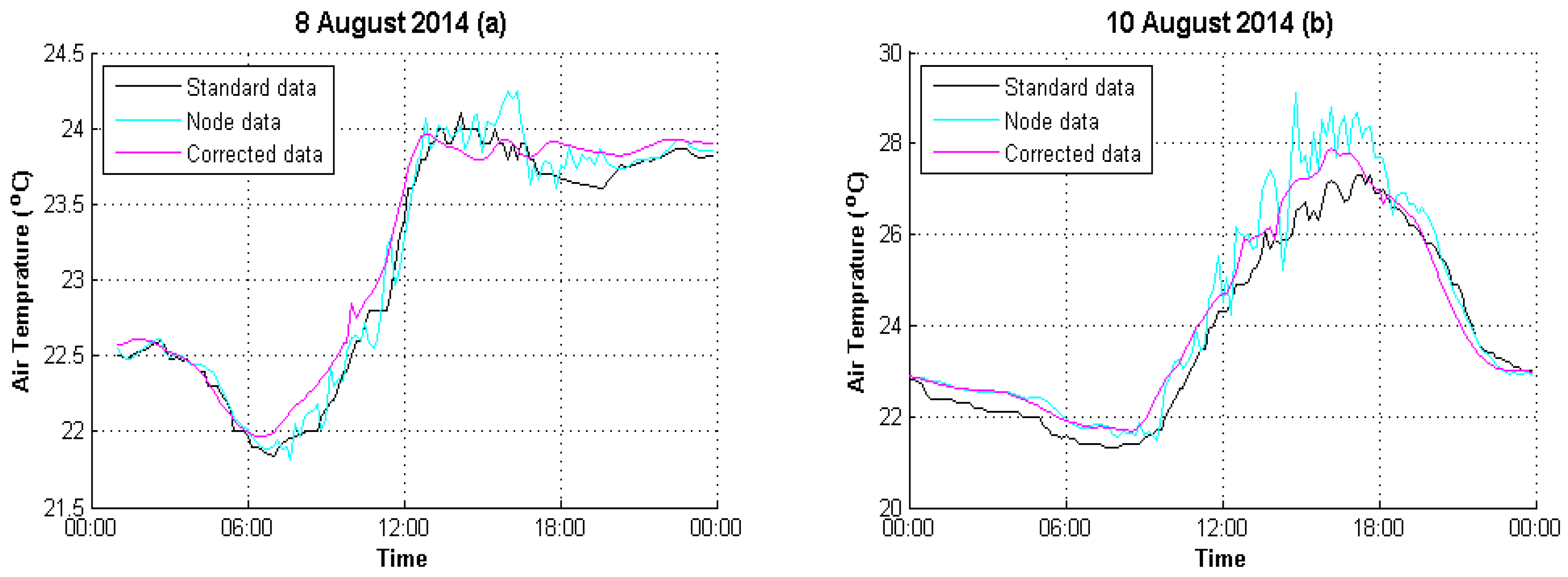
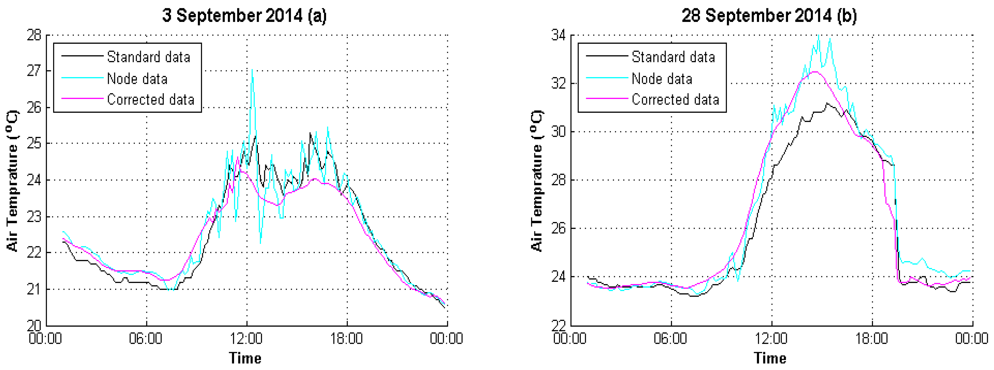
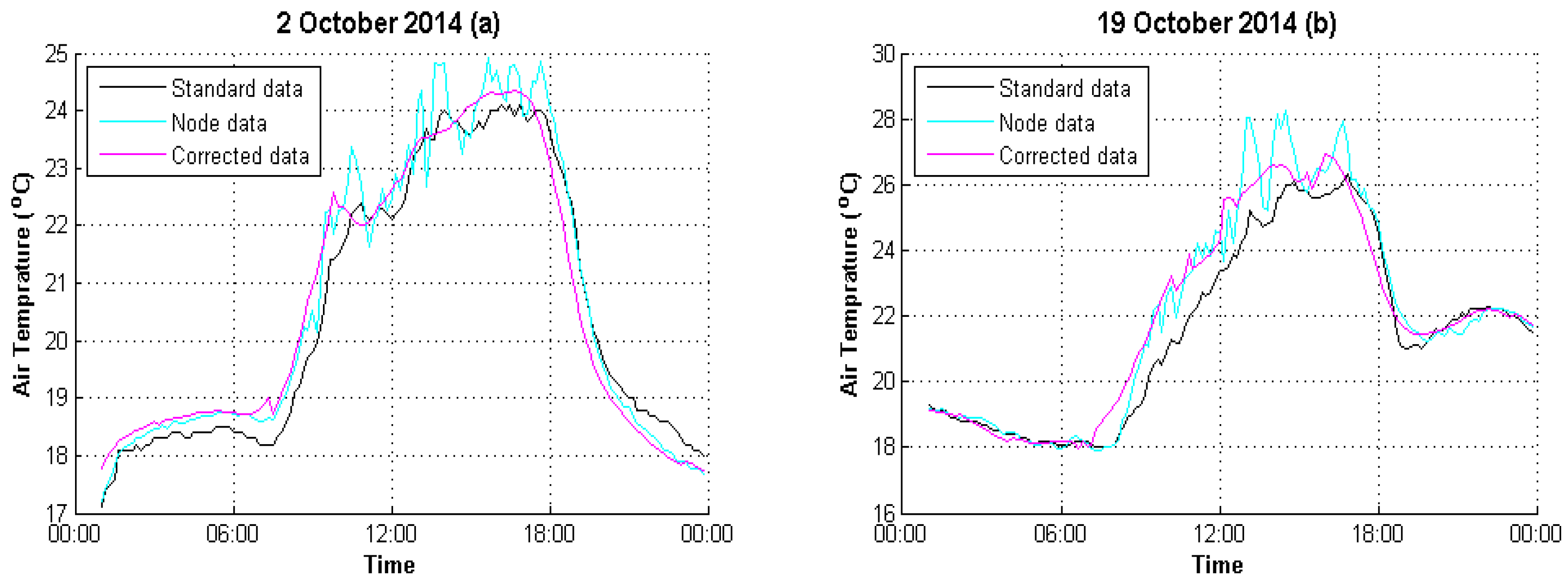
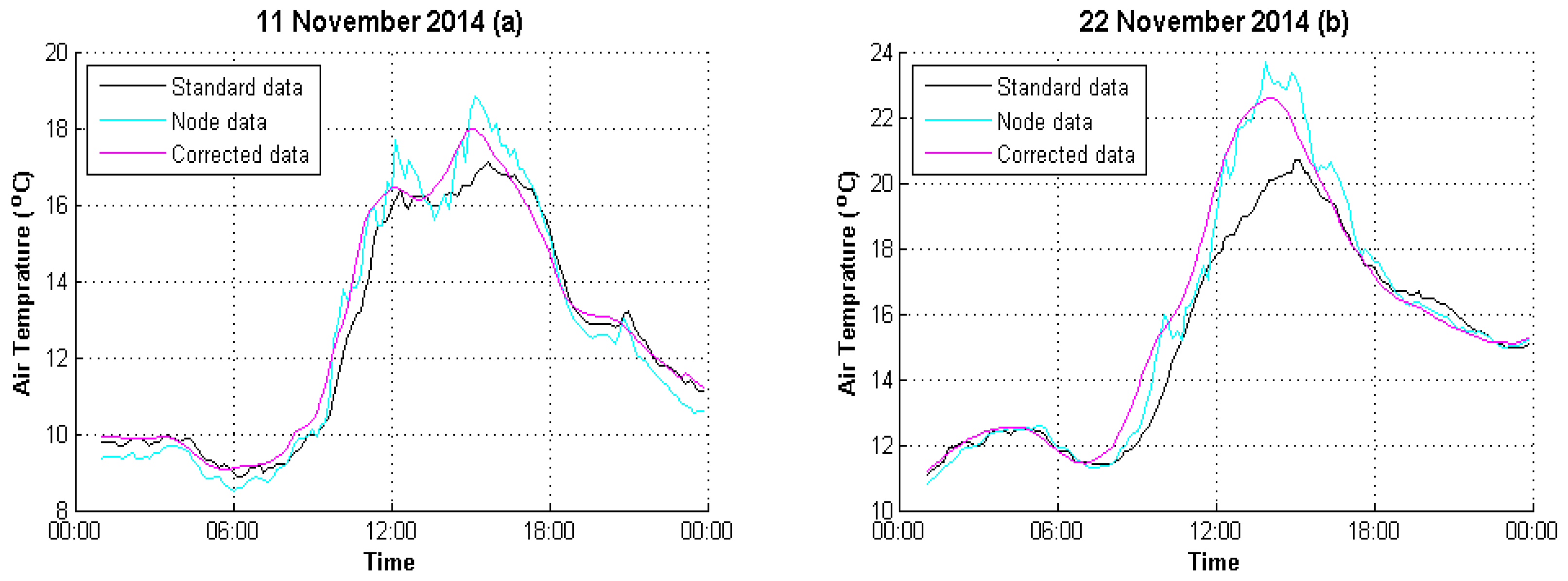
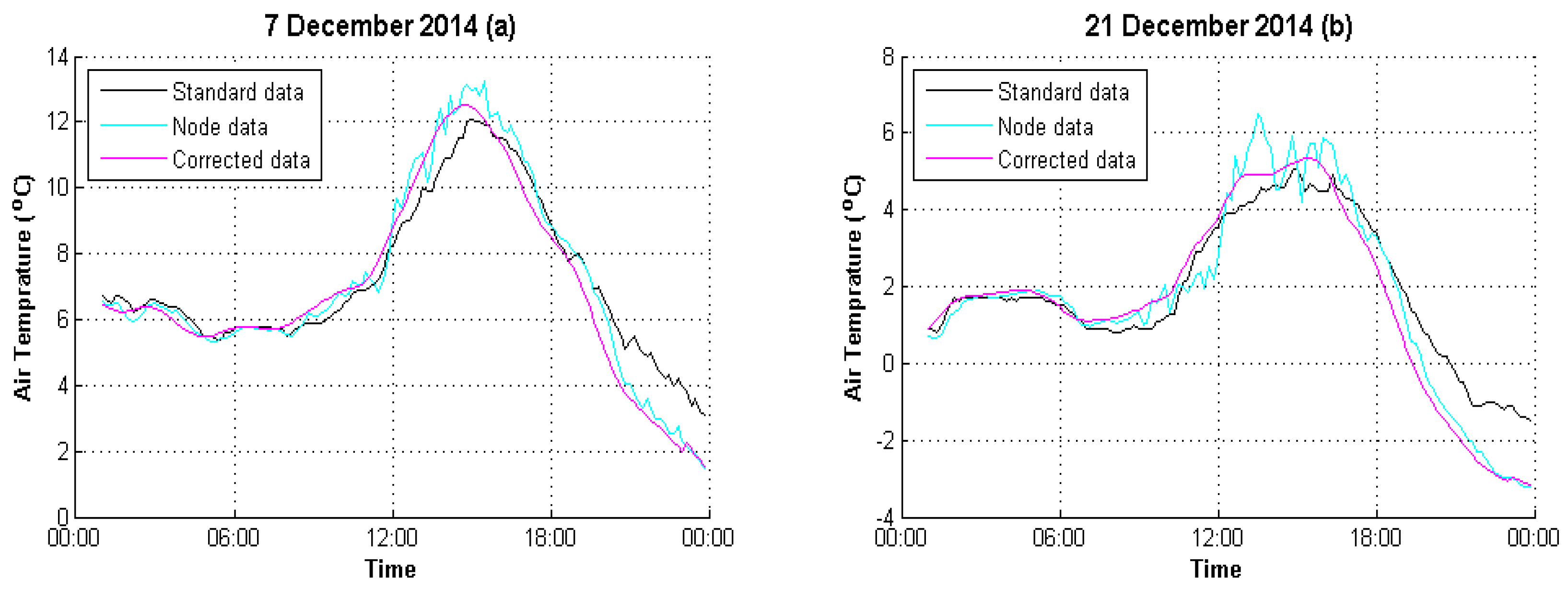
In order to show the results of this paper more clearly and intuitively, we selected two days per month from June to December 2014 to illustrate the results of the corrected node data. As shown in Figure 4, Figure 5, Figure 6, Figure 7, Figure 8, Figure 9 and Figure 10, the confidence interval and the predicted values are removed. The black line represents the standard temperature data, the blue line represents the node data after the initial correction and the purple line represents the corrected node data.
As we can see from Figure 5, Figure 6, Figure 7, Figure 8, Figure 9, Figure 10 and Figure 11, the corrected node data curve becomes relatively smooth and the drastic changes of local data are also greatly reduced. At the same time, it also keeps the trend of temperature change, which is closer to the standard data than the original data. In order to illustrate the efficiency of the algorithm in more detail, we refer to Root Mean Square Error (RMSE), Symmetric Mean Absolute Percentage Error (SMAPE) and the Pearson’s Correlation Coefficient (R2) to prove the efficiency of the algorithm in this paper.
RMSE is very sensitive to the large or small errors in a set of measurements. Therefore, RMSE can reflect well the precision of the measurement. Table 1 presents the root mean square error between standard data and node data before and after correction. The smaller the value of RMSE is, the higher the accuracy is.
In Table 2, we present the the Pearson’s Correlation Coefficient between sensed data and standard data. In statistics, the Pearson’s Correlation Coefficient is a measure of the linear correlation between two variables X and Y. It is widely used in the sciences as a measure of the degree of linear dependence between two variables and can be used to measure the correlation between node data and standard data. As we can see in the column “Raw Data” in Table 2, the correlation coefficients between uncorrected node data and standard data are not high. This means a low correlation degree between unprocessed data and standard data. However, the coefficients are improved after the process of value correcting.
When comparing how well different algorithms forecast time series, researchers use an average value of the ratio, known as the Symmetric Mean Absolute Percentage Error (SMAPE). The lower the ratio, the better the prediction. Table 3 presents the Symmetric Mean Absolute Percentage Errors on every whole day. As we can see, the error rate of the corrected node temperature data is already very low.
For our method, it can be inferred that the anomalies can be effectively detected by the window-based forecasting model, which is constructed using the AR prediction model. The average values of RMSE, SMAPE and R2 after correction are 0.4881, 2.83% and 0.9892, respectively. The results suggest that there is a remarkable improvement in the detection and correction performance on the raw dataset. The most important thing is that most of the corrected data can be guaranteed within the allowable error range. Thus, the results show that the algorithm is effective and practical.

5. Conclusions

In this paper, the outliers in the temperature time series of meteorological sensor networks are studied. A sliding window based prediction algorithm is proposed to detect outliers in the temperature time series. The dynamic parameter selection method is used to select the optimal parameters to establish the correction model. The temperature data measured by the low cost meteorological sensor network are tested and the correction results are compared with the standard temperature to calculate the correction efficiency. The results show that the algorithm can accurately detect the outliers in time series and correct them. Although there is no significant improvement in the index of Mean Absolute Error, it can still be reduced by many ways such as data translation. At present, the node data has basically met the requirements of meteorological data quality control, which is convenient for later analysis.

Acknowledgments

This work is supported by the National Science Foundation of China under Grant No. 61173136, U1536206, 61232016, U1405254, 61373133, 61502242, the Jiangsu Government Scholarship for Overseas Studies under Grant JS-2014-351, the CICAEET (Jiangsu Collaborative Innovation Center on Atmospheric Environment and Equipment Technology) fund and PAPD (Priority Academic Program Development of Jiangsu Higher Education Institutions) fund.

Author Contributions

X.G. and L.M. conceived and designed the experiments; X.G. performed the experiments; X.G. analyzed the data; B.W. contributed reagents/materials/analysis tools; X.G. wrote the paper.

Conflicts of Interest

The authors declare no conflict of interest.

References

  1. Tan, J.; Yang, L.; Grimmond, C.S.B.; Shi, J.; Gu, W.; Chang, Y.; Hu, P.; Sun, J.; Ao, X.; Han, Z. Urban Integrated Meteorological Observations: Practice and Experience in Shanghai, China. Bull. Am. Meteorol. Soc. 2015, 96, 197–210. [Google Scholar] [CrossRef]
  2. Sigsgaard, E.E.; Carl, H.; Møller, P.R.; Thomsen, P.F. Monitoring the near-extinct European weather loach in Denmark based on environmental DNA from water samples. Biol. Conserv. 2015, 183, 46–52. [Google Scholar] [CrossRef]
  3. Chandran, M.A.S.; Rao, A.V.M.S.; Sandeep, V.M.; Pramod, V.P.; Pani, P.; Rao, V.U.M.; Kumari, V.V.; Rao, C.S. Indian summer heat wave of 2015: A biometeorological analysis using half hourly automatic weather station data with special reference to Andhra Pradesh. Int. J. Biometeorol. 2016, 1–10. [Google Scholar] [CrossRef] [PubMed]
  4. Liu, W.; Wang, C.L.; Chen, X.G.; Chen, H.H. Characteristics of heat resource in mountainous region of northern Guangdong, South China based on three-dimensional climate observation. Chin. J. Appl. Ecol. 2013, 24, 2571–2580. (In Chinese) [Google Scholar]
  5. Xie, S.; Wang, Y. Construction of Tree Network with Limited Delivery Latency in Homogeneous Wireless Sensor Networks. Wirel. Pers. Commun. 2014, 78, 231–246. [Google Scholar] [CrossRef]
  6. Wang, L.; Xu, L.D.; Bi, Z.; Xu, Y. Data Cleaning for RFID and WSN Integration. IEEE Trans. Ind. Inform. 2014, 10, 408–418. [Google Scholar] [CrossRef]
  7. Padmavathi, G.; Shanmugapriya, D.; Kalaivani, M. A Study on Vehicle Detection and Tracking Using Wireless Sensor Networks. Wirel. Sens. Netw. 2010, 2, 173–185. [Google Scholar] [CrossRef]
  8. Nijak, G. M.J.; Geary, J.R.; Larson, S.L.; Talley, J.W. Autonomous, wireless in-situ sensor (AWISS) for rapid warning of Escherichia coli outbreaks in recreational and source waters. Environ. Eng. Sci. 2012, 29, 64–69. [Google Scholar] [CrossRef]
  9. Park, P.; Marco, P.D.; Johansson, K. Cross-Layer Optimization for Industrial Control Applications using Wireless Sensor and Actuator Mesh Networks. IEEE Trans. Ind. Electron. 2017, 64, 3250–3259. [Google Scholar] [CrossRef]
  10. Kong, D.; Li, T.; You, X.; Sun, X.; Wang, B.; Liu, Q. The Research of Long-Distance Data Transmission Based on Meteorological Sensor Network. Int. J. Future Gener. Commun. Netw. 2014, 7, 59–70. [Google Scholar] [CrossRef]
  11. Nagy, Z.; Rossi, D.; Hersberger, C.; Irigoyen, S.D.; Miller, C.; Schlueter, A. Balancing envelope and heating system parameters for zero emissions retrofit using building sensor data. Appl. Energy 2014, 131, 56–66. [Google Scholar] [CrossRef]
  12. Sun, X.; Yan, S.; Wang, B.; Li, X.; Liu, Q.; Zhang, H. Air Temperature Error Correction Based on Solar Radiation in an Economical Meteorological Wireless Sensor Network. Sensors 2015, 15, 18114–18139. [Google Scholar] [CrossRef] [PubMed]
  13. Dai, H.J.; Touray, M.; Jonnagaddala, J.; Syed-Abdul, S. Feature Engineering for Recognizing Adverse Drug Reactions from Twitter Posts. Information 2016, 7, 27. [Google Scholar] [CrossRef]
  14. Esling, P.; Agon, C. Time-series data mining. ACM Comput. Surv. 2012, 45, 12. [Google Scholar] [CrossRef]
  15. Sun, W.; Ishidaira, H.; Bastola, S.; Yu, J. Estimating daily time series of streamflow using hydrological model calibrated based on satellite observations of river water surface width: Toward real world applications. Environ. Res. 2015, 139, 36–45. [Google Scholar] [CrossRef] [PubMed]
  16. Wright, A.P.; Wright, A.T.; Mccoy, A.B.; Sittig, D.F. The use of sequential pattern mining to predict next prescribed medications. J. Biomed. Inform. 2015, 53, 73–80. [Google Scholar] [CrossRef] [PubMed]
  17. Ruuskanen, V.; Nerg, J.; Pyrhonen, J.; Ruotsalainen, S. Drive Cycle Analysis of a Permanent-Magnet Traction Motor Based on Magnetostatic Finite-Element Analysis. IEEE Trans. Veh. Technol. 2015, 64, 1249–1254. [Google Scholar] [CrossRef]
  18. Liu, H.; Wang, B.; Sun, X.; Li, T.; Liu, Q.; Guo, Y. DCSCS: A Novel Approach to Improve Data Accuracy for Low Cost Meteorological Sensor Networks. Inf. Technol. J. 2014, 13, 1640–1647. [Google Scholar]
  19. Hawkins, D.M. Identification of Outliers. Biometrics 1980, 37, 860. [Google Scholar]
  20. Chandola, V.; Banerjee, A.; Kumar, V. Anomaly detection: A survey. ACM Comput. Surv. 2009, 41, 1–58. [Google Scholar] [CrossRef]
  21. Laber, E.B.; Zhao, Y.Q. Outlier detection for high-dimensional data. Biometrika 2015, 102, 589–599. [Google Scholar]
  22. Gogoi, P.; Bhattacharyya, D.K.; Borah, B.; Kalita, J.K. A Survey of Outlier Detection Methods in Network Anomaly Identification. Comput. J. 2011, 54, 570–588. [Google Scholar] [CrossRef]
  23. Wu, T.B.; Cheng, Y.; Hu, Z.K.; Xie, W.P.; Liu, Y.L. A New PLS and Bayesian Classification Based On-Line Outlier Detection Method. Appl. Mech. Mater. 2013, 397–400, 1362–1365. [Google Scholar] [CrossRef]
  24. Wang, X.; Wang, X.L.; Ma, Y.; Wilkes, D.M. A fast MST-inspired kNN-based outlier detection method. Inf. Syst. 2015, 48, 89–112. [Google Scholar] [CrossRef]
  25. Tsai, C.F.; Cheng, K.C. Simple instance selection for bankruptcy prediction. Knowl.-Based Syst. 2012, 27, 333–342. [Google Scholar] [CrossRef]
  26. Liu, J.; Deng, H.F. Outlier detection on uncertain data based on local information. Knowl.-Based Syst. 2013, 51, 60–71. [Google Scholar] [CrossRef]
  27. Cassisi, C.; Ferro, A.; Giugno, R.; Pigola, G.; Pulvirenti, A. Enhancing density-based clustering: Parameter reduction and outlier detection. Inf. Syst. 2013, 38, 317–330. [Google Scholar] [CrossRef]
  28. Shahid, N.; Naqvi, I.H.; Qaisar, S.B. One-class support vector machines: Analysis of outlier detection for wireless sensor networks in harsh environments. Artif. Intell. Rev. 2015, 43, 515–563. [Google Scholar] [CrossRef]
  29. Dufrenois, F.; Noyer, J.C. One class proximal support vector machines. Pattern Recogn. 2016, 52, 96–112. [Google Scholar] [CrossRef]
  30. Jiang, F.; Liu, G.; Du, J.; Sui, Y. Initialization of K-modes clustering using outlier detection techniques. Inf. Sci. 2016, 332, 167–183. [Google Scholar] [CrossRef]
  31. Jobe, J.M.; Pokojovy, M. A Cluster-Based Outlier Detection Scheme for Multivariate Data. J. Am. Stat. Assoc. 2015, 110, 1543–1551. [Google Scholar] [CrossRef]
  32. Hill, D.J.; Minsker, B.S. Anomaly detection in streaming environmental sensor data: A data-driven modeling approach. Environ. Model. Softw. 2010, 25, 1014–1022. [Google Scholar] [CrossRef]
  33. Zhao, N.; Yu, F.R.; Sun, H.; Yin, H.; Nallanathan, A.; Wang, G. Interference alignment with delayed channel state information and dynamic AR-model channel prediction in wireless networks. Wirel. Netw. 2015, 21, 1227–1242. [Google Scholar] [CrossRef]
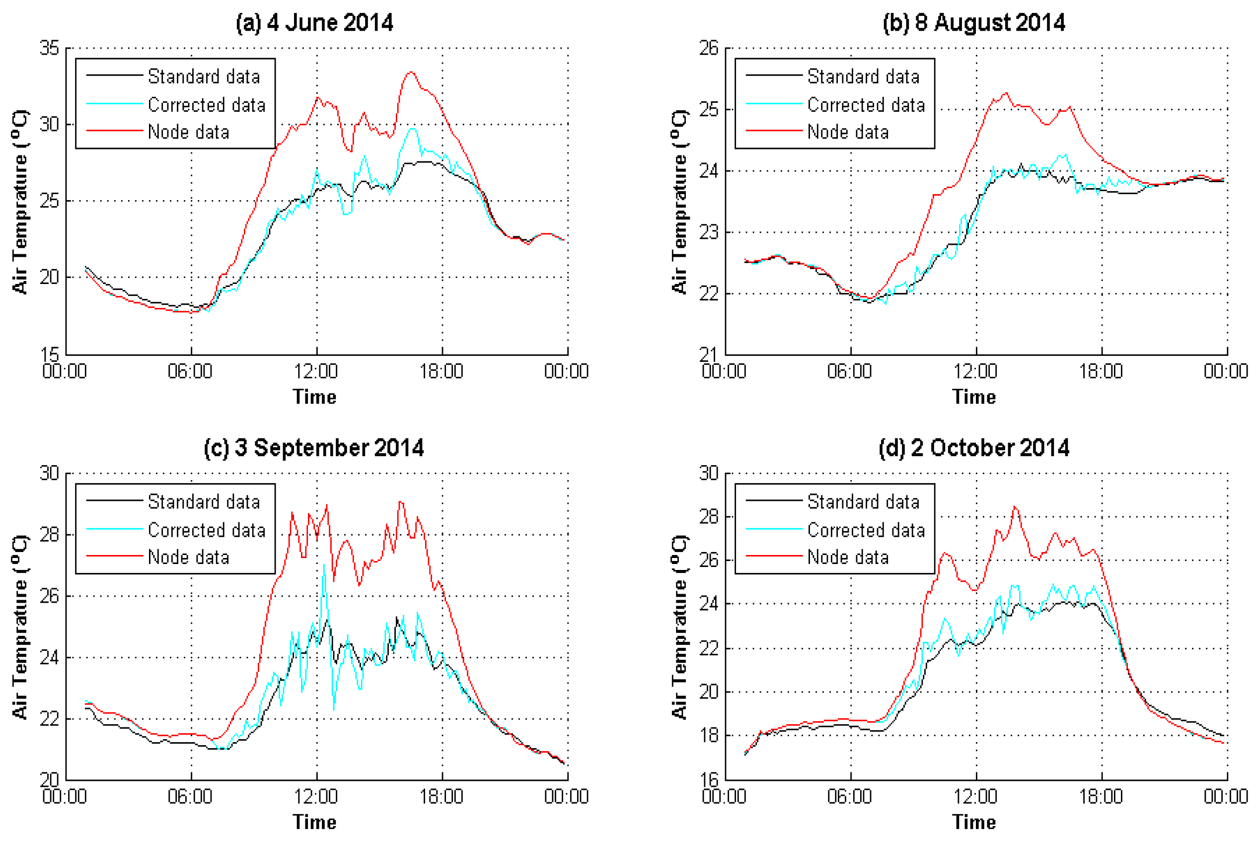
Figure 1. Corrected results of node data using solar radiation in four days. (a) 4 June 2014; (b) 8 August 2014; (c) 3 September 2014; (d) 2 October 2014.
Information 08 00060 g001
Figure 2. Outlier detection and correction algorithm based on a sliding window.
Information 08 00060 g002
Figure 3. Temperature data on 4 June 2014.
Information 08 00060 g003
Figure 4. Outlier detection and correction results in (k, p) = (5, 95%).
Information 08 00060 g004
Figure 5. Revised results on 4 June 2014 (a) and 9 June 2014 (b).
Information 08 00060 g005
Figure 6. Revised results on 4 July 2014 (a) and 7 July 2014 (b).
Information 08 00060 g006
Figure 7. Revised results on 8 August 2014 (a) and 10 August 2014 (b).
Information 08 00060 g007
Figure 8. Revised results on 3 September 2014 (a) and 28 September 2014 (b).
Information 08 00060 g008
Figure 9. Revised results on 2 October 2014 (a) and 19 October 2014 (b).
Information 08 00060 g009
Figure 10. Revised results on 11 November 2014 (a) and 22 November 2014 (b).
Information 08 00060 g010
Figure 11. Revised results on 7 December 2014 (a) and 21 December 2014 (b).
Information 08 00060 g011
Table 1. Root Mean Square Error (RMSE) before and after correction.
DateRoot Mean Square Error
Raw DataCorrected Data
4 June 20142.97060.4432
9 June 20143.44100.2883
4 July 20140.87660.1910
7 July 20143.43760.8598
8 August 20140.64960.1199
10 August 20142.66650.3984
3 September 20142.14790.4458
28 September 20143.20440.5826
2 October 20141.98830.3169
19 October 20142.69070.5654
11 November 20142.09040.3317
22 November 20142.66580.9391
7 December 20142.10440.6247
21 December 20142.01930.6711
Average2.16340.4811
Table 2. Correlation coefficient between node data and standard data.
DateCorrelation Coefficient
Raw DataCorrected Data
4 June 20140.95650.9935
9 June 20140.90240.9968
4 July 20140.94370.9931
7 July 20140.94540.9855
8 August 20140.90990.9917
10 August 20140.92540.9932
3 September 20140.96850.9725
28 September 20140.94940.9944
2 October 20140.97630.9922
19 October 20140.93330.9911
11 November 20140.95640.9972
22 November 20140.94480.9843
7 December 20140.97050.9863
21 December 20140.96880.9773
Average0.94650.9892
Table 3. Comparison of Symmetric Mean Absolute Percentage Error before and after correction.
DateSymmetric Mean Absolute Percentage Error (SMAPE)
Raw DataCorrected Data
4 June 20148.1%1.56%
9 June 20147.76%0.77%
4 July 20142.59%0.64%
7 July 20148.85%2.41%
8 August 20141.93%0.43%
10 August 20146.74%1.42%
3 September 20146.13%1.44%
28 September 20146.79%1.34%
2 October 20146.05%1.38%
19 October 20147.02%1.83%
11 November 20148.71%1.63%
22 November 20148.12%3.32%
7 December 201417.09%8.33%
21 December 201415.17%13.06%
Average7.93%2.83%