Improved Genetic Algorithm Optimization for Forward Vehicle Detection Problems

Abstract

Automated forward vehicle detection is an integral component of many advanced driver-assistance systems. The method based on multi-visual information fusion, with its exclusive advantages, has become one of the important topics in this research field. During the whole detection process, there are two key points that should to be resolved. One is to find the robust features for identification and the other is to apply an efficient algorithm for training the model designed with multi-information. This paper presents an adaptive SVM (Support Vector Machine) model to detect vehicle with range estimation using an on-board camera. Due to the extrinsic factors such as shadows and illumination, we pay more attention to enhancing the system with several robust features extracted from a real driving environment. Then, with the introduction of an improved genetic algorithm, the features are fused efficiently by the proposed SVM model. In order to apply the model in the forward collision warning system, longitudinal distance information is provided simultaneously. The proposed method is successfully implemented on a test car and evaluation experimental results show reliability in terms of both the detection rate and potential effectiveness in a real-driving environment.

1. Introduction

As an important component of ADAS, FCWS has received considerable attention in recent decades due to the fact many accidents are caused mainly by drivers’ lack of attention or fatigue. FCWS is an on-board system which can warn the driver of a potential vehicle collision risk in front of the host vehicle. If car drivers have a 0.5-second additional warning time, about 60% of rear-end collisions can be prevented. An extra second of warning time can prevent about 90% of rear-end collisions [1]. Thus, FCWS has been considered as an important application for improving traffic safety and accident prevention.

Since the forward vehicle detection plays a more important role in FCWS, which has been extensively studied using various sensors. Researches indicate that the sensors used widely can be roughly classified into two main types: active sensors and camera sensors. In early stages, active sensors such as radar and LiDAR are used [2,3]. The main advantage is that the sensors can achieve a reliable distance even in rain or fog, where average drivers have a visibility of 10 m or less. However, on the contrary, the high cost, low spatial resolution, narrow field of view and unitary information have restricted their use in practical applications. In recent years, camera sensors are being widely used due to the reasons mentioned above [4,5]. This method overcomes the limitations of active sensors and furthermore can be used in a wider range of applications, such as in lane departure warning systems and event video recorders. These advantages are conducive not only to achieving more robust detection result, but also to the ADAS equipment integration with multifunction in the future.

Vehicles have a wide variety of appearances such as shape, color, size and textures, etc. How to use these information and enhance the system efficiency is a big challenge in practical applications. Therefore, at present, very few products are developed for real driving environments even if there are so many researches and huge market demands.

Generally, previous researches extract the vehicle features with prior knowledge cues and then verify the candidates with conventional classification algorithms. In which, reasonable and effective feature extraction is important for the detection phase. For this purpose, various prior knowledge such as shadow, symmetry, color, edge and texture are used [6,7,8,9,10]. In ref [6], shadow and edge information are used. Several sequences from real driving environments have been tested and have obtained highly accurate results. However, the most serious drawback of this research is that it may be unreliable in the scenes with low sun, making vehicles cast long shadows, and leading to interference from shadow of leaves. Mithun [10] proposed a novel detection and classification method by utilizing the shape-based, shape-invariant and texture-based features. Experimental results demonstrate that the proposed method provides a significant improvement in counting and classifying the vehicles in terms of accuracy and robustness alongside a substantial reduction of execution time. In fact, this method belongs to the video-based method for moving object detection [11,12]. In addition, generally, texture feature extraction is a time-consuming task due to the complex computation process. Thus, this method is impractical for a real-time application. However, the accurate and effective demonstration for object detection motivates us to apply it into this paper’s research tasks. How to reduce the computation complexity so as to improve the system performance is a primary problem to be solved.

Once the robust features for vehicle detection are obtained, the next step is identifying the candidates extracted with a classification method such as artificial neural network, SVM, and AdaBoost. SVM, a novel supervised learning method used for classification and regression, has been recently proved to be a promising tool for both data classification and pattern recognition [13,14,15]. SVM has been shown to be very resistant to the over-fitting problem, achieving high generalization performance in solving various time series forecasting problems, which has been applied in prediction of time series [16,17]. These successful applications motivate us to apply SVM in this paper’s research.

The purpose of this paper is to establish an adaptive GA-SVM model for forward vehicle detection in real driving environments. Within the proposed model, in order to enhance the system robustness, several features including invariant moments and textures are considered. During the model training process, this paper adopts an improved GA algorithm to improve the training efficiency. This paper aims to make two contributions to the literature. Firstly, it attempts to make the proposed model adaptive to various lighting conditions, even in the environment with interference of leave shadows. Secondly, it tries to promote the model training efficiency with an improved SVM model. It is expected to help enhance the model accuracy with limited experimental data.

2. System Overview

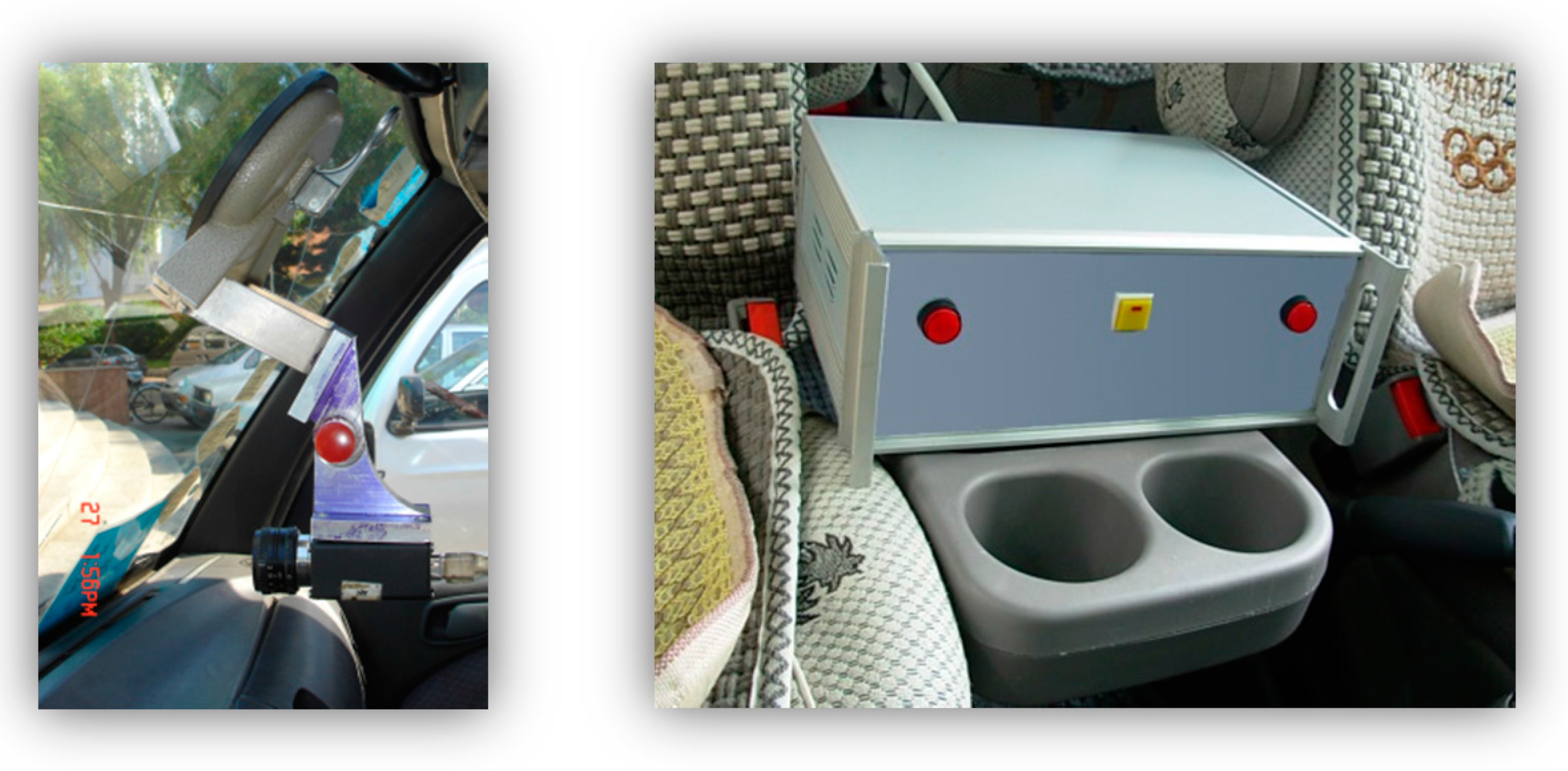
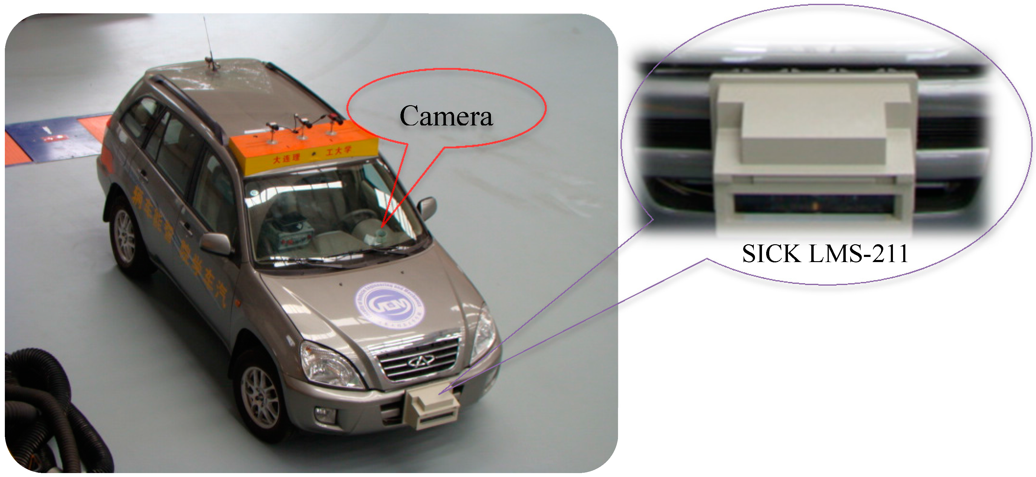
2.1. On-Board System Setup

To obtain the road scenario, an image acquiring system will be needed. The configuration for the proposed system consists of a camera and on-board computer, as shown in Figure 1. When the system is started, the camera mounted on the windshield captures the road image and transmits it to a computer in real time. Then, the image is processed using the proposed algorithm.

Figure 1. Hardware configuration for the proposed method.

Figure 1. Hardware configuration for the proposed method.

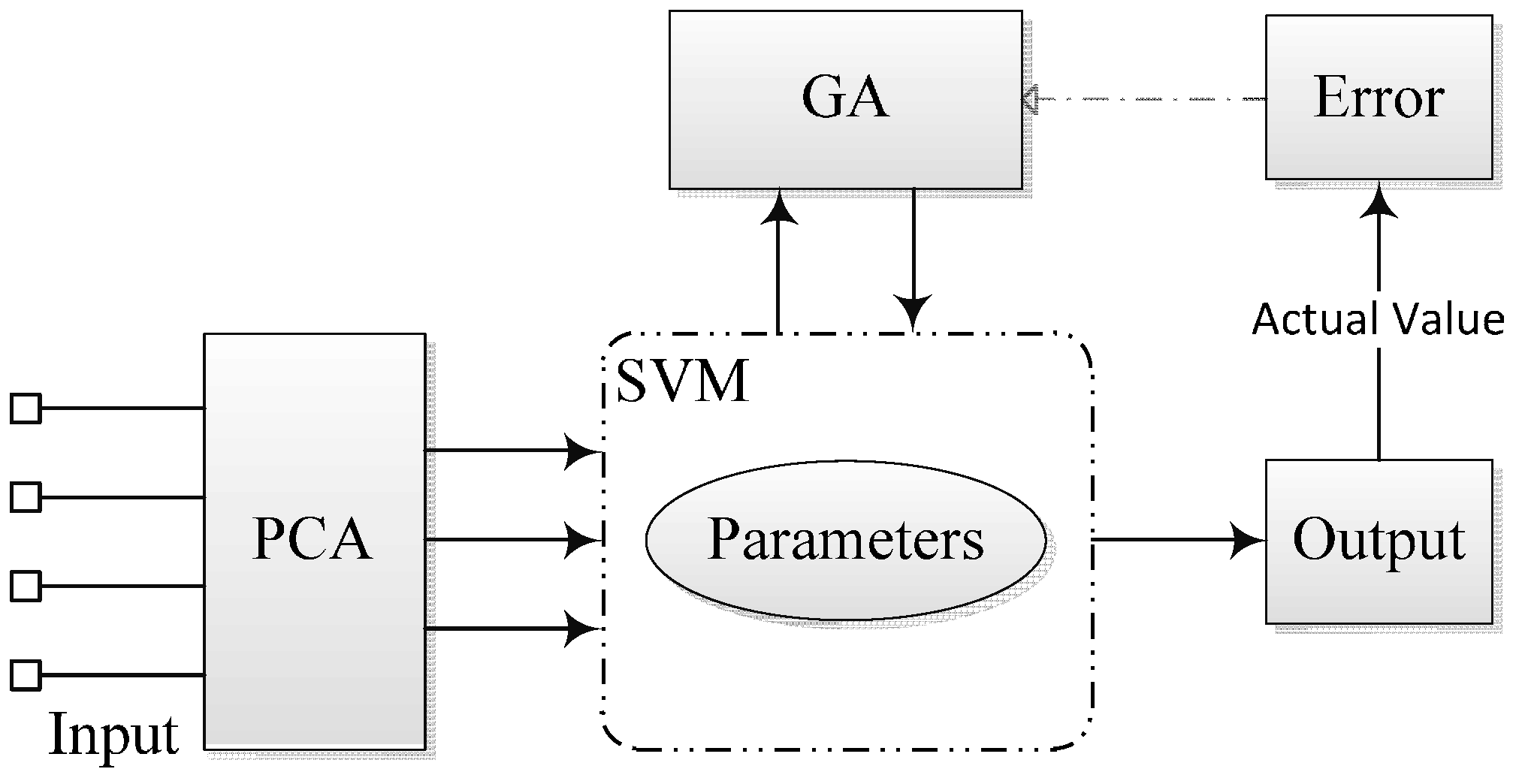
2.2. Overview of the Proposed Method

Considering the performance required in practical applications, the proposed program refined vehicle detection algorithm is shown in Figure 2.

Firstly, image preprocessing steps dedicated to reduce Gaussian and Pepper noise are applied. Then, the region of interest (ROI), in which vehicles possibly appear, is defined based on lane detection. In this region, many unnecessary influences (e.g., lamps, traffic lights, signs, etc.) outside the ROI are excluded. In order to improve detection accuracy, the moment and texture features of candidates are used for the proposed SVM model. For the system tracking process, Camshift algorithm is adopted to find the “target” in the ROI effectively.

Figure 2. Flow chart of the forward vehicle detection.

Figure 2. Flow chart of the forward vehicle detection.

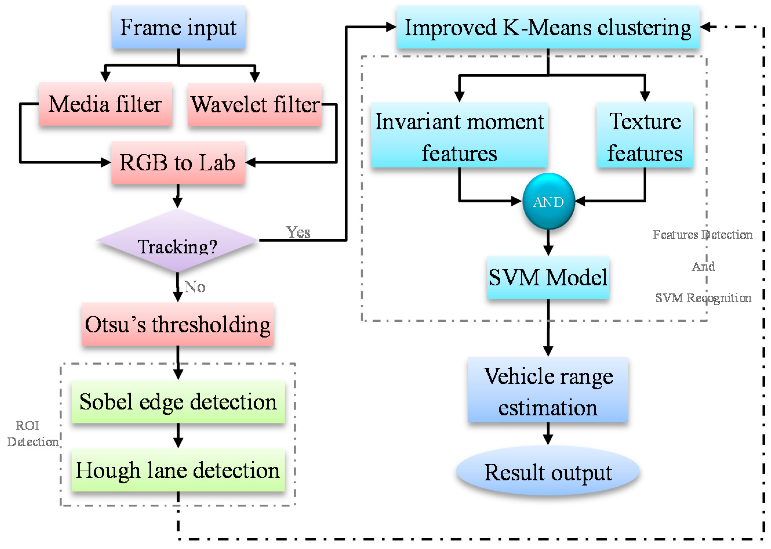
3. Vehicle Detection Using SVM

3.1. Hypothesis Generation

In the hypothesis generation step, image preprocess steps are conducted in order to reduce the interference from Gaussian and Pepper noise which occurs commonly in real-driving environments. Within the defined ROI, based on the common features that vehicles always cause shadow on the road [18], the shadow underneath the vehicles is detected. Then, the vehicle bottom lines, where the vehicle and road meet, are extracted. With these lines, vehicle candidates can be successfully extracted. Figure 3 shows the overall process for candidates’ extraction in the hypothesis generation step.

Figure 3. Flow chart of the forward vehicle candidate detection.

Figure 3. Flow chart of the forward vehicle candidate detection.

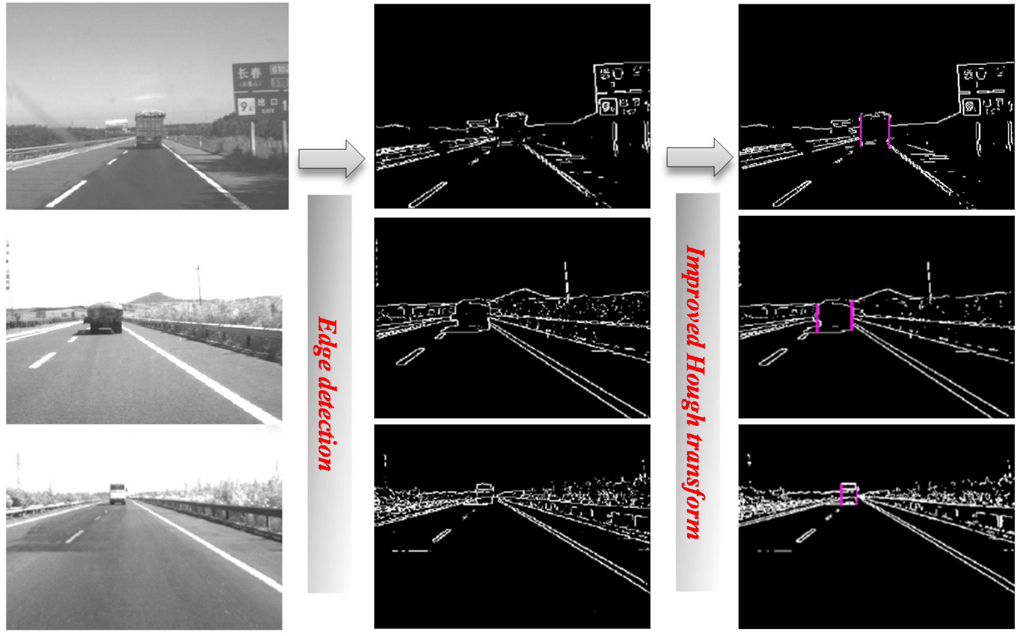
3.1.1. Hypothesis Generation: Image Preprocess and Segmentation

To reduce Gaussian and Pepper noise, tests are carried out with various filters. From Table 1, it can be seen that the median filter is effective for reducing the pepper noise and wavelet filter for Gaussian. So, in this paper, median and compromise threshold wavelet filters are adopted.

Table 1. Statistical analysis result.

Filter	Mask size	SNR (db)	RMSE
Original image	——	5.51	0.24
Median filter	3 × 3	5.94	0.22
Mean filter	3 × 3	5.54	0.23
Wiener filter	3 × 3	5.98	0.22
Wavelet filter	Soft threshold	7.83	0.31
	Hard threshold	12.37	0.19
	Compromise threshold	31.07	0.02

Table 1. Statistical analysis result.

Filter	Mask size	SNR (db)	RMSE
Original image	——	5.51	0.24
Median filter	3 × 3	5.94	0.22
Mean filter	3 × 3	5.54	0.23
Wiener filter	3 × 3	5.98	0.22
Wavelet filter	Soft threshold	7.83	0.31
	Hard threshold	12.37	0.19
	Compromise threshold	31.07	0.02

In computer vision and image processing, Otsu’s method is used to automatically perform histogram shape-based image segmentation or the reduction of a gray image to a binary image. In addition, it is proved one of the best methods for threshold selection [19]. Therefore, in this paper, we segment the vehicle image with L component in Lab color space based on this method.

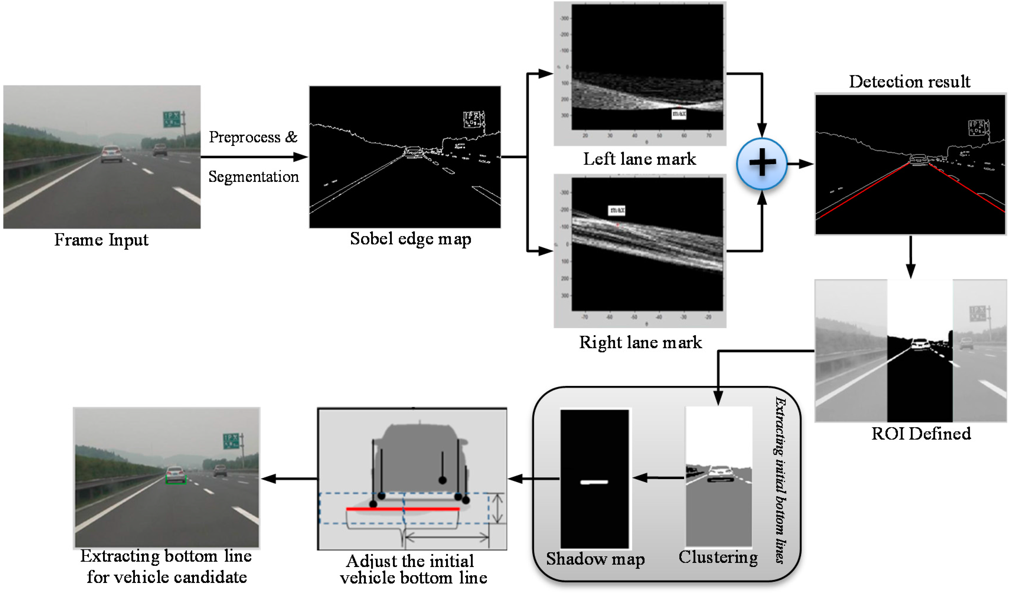
3.1.2. Hypothesis Generation: Lane Detection and ROI Defining

Previous research shows that Hough transform (HT) is not sensitive to noise and handles the incomplete or partially covered target [20]. For real time application, there are two key steps that need to be undertaken. One is the robust edge map extraction and the other is HT parameters’ range design. The former is the basis for correct lane detection and the latter can improve the efficiency of the parameter search process.

In a real driving environment, horizontal and vertical edge maps should be responsive to illumination changes. So, the proposed method computes the 1st-order derivative of image intensity, followed by the adaptive threshold. As the contrast tends to be proportional to illumination, the local mean intensity is used to set the adaptive threshold value. The edge maps are calculated as follows:

$$E{M}_H(p)=\{\begin{array}{l}\begin{array}{cc}1,& \left|G_H(p)\right|>\frac{a}{m}{\displaystyle \sum _{p\in \text{Ω}}f(p)}\end{array}\hfill \\ \begin{array}{ll}0,\hfill & otherwise\hfill \end{array}\hfill \end{array}$$

(1)

$$E{M}_V(p)=\{\begin{array}{l}\begin{array}{cc}1,& \left|G_V(p)\right|>\frac{a}{m}{\displaystyle \sum _{p\in \text{Ω}}f(p)}\end{array}\hfill \\ \begin{array}{cc}0,& otherwise\end{array}\hfill \end{array}$$

(2)

where $E{M}_H(p)$ and $E{M}_V(p)$ represent the horizontal and vertical binary edge maps at pixel p, respectively. $G_H(p)$ and $G_V(p)$ are the results of Sobel edge detectors. $\text{Ω}$ is the neighborhood set of the Sobel filter, m is the number of pixels in the neighborhood set, and a is a constant to adjust the sensitivity of the edge response. The proposed method is able to build the binary edge maps robustly even if the illumination condition has been changed.

Since the parameters range design is important for lane detection using HT method. In this paper, the image is divided into two regions; the origin point is set at the bottom center, as shown in Figure 4. For each region, given line equation $y=kx+b$, the HT is carried out by the following equation:

$$r=x\cos \left(\theta \right)+y\sin \left(\theta \right)$$

(3)

where, (r, θ) is the vector from the origin to the nearest point of line $y=kx+b$. According to our experience, the range of parameter θ is set with $[{15}^{°},{75}^{°}]$. With the proposed method, several samples obtained from a real driving environment are conducted. Results show that, in tracking mode, the method can detect lane with an average accuracy 90% and 30 ms time-consumption per frame.

Figure 4. Flow chart of the forward vehicle candidate detection.

Figure 4. Flow chart of the forward vehicle candidate detection.

In a real driving environment, most collision accidents are rear-ending collisions in the current lane. Thus, the ROI (defined as Figure 5) near the vanishing point is set to minimize the impact from other objects and improve system performance. The left and right boundaries are defined as the boundary which are 1.5 times the distance from vanishing point to intersection point, respectively.

Figure 5. Vanishing point and ROI definition.

Figure 5. Vanishing point and ROI definition.

It is important to note that the intersection points are important cues for the subsequent initial vehicle bottom line extraction. For example, when the low sun castes long shadows underneath the vehicle, the proposed method based on shadow detection always achieves a failed result. So, subject to the constraints of intersection point mentioned above, we can achieve a more accurate shadow detection result than the method in [6]. Furthermore, this paper defines the ROI area differently from the reference due to the fact that in the lower-triangular area (as ref [6] used), the process complexity can be reduced efficiently, but more useful information such as the vehicle rear-end texture is lost. Unfortunately, these cues are essential for the vehicle verification step.

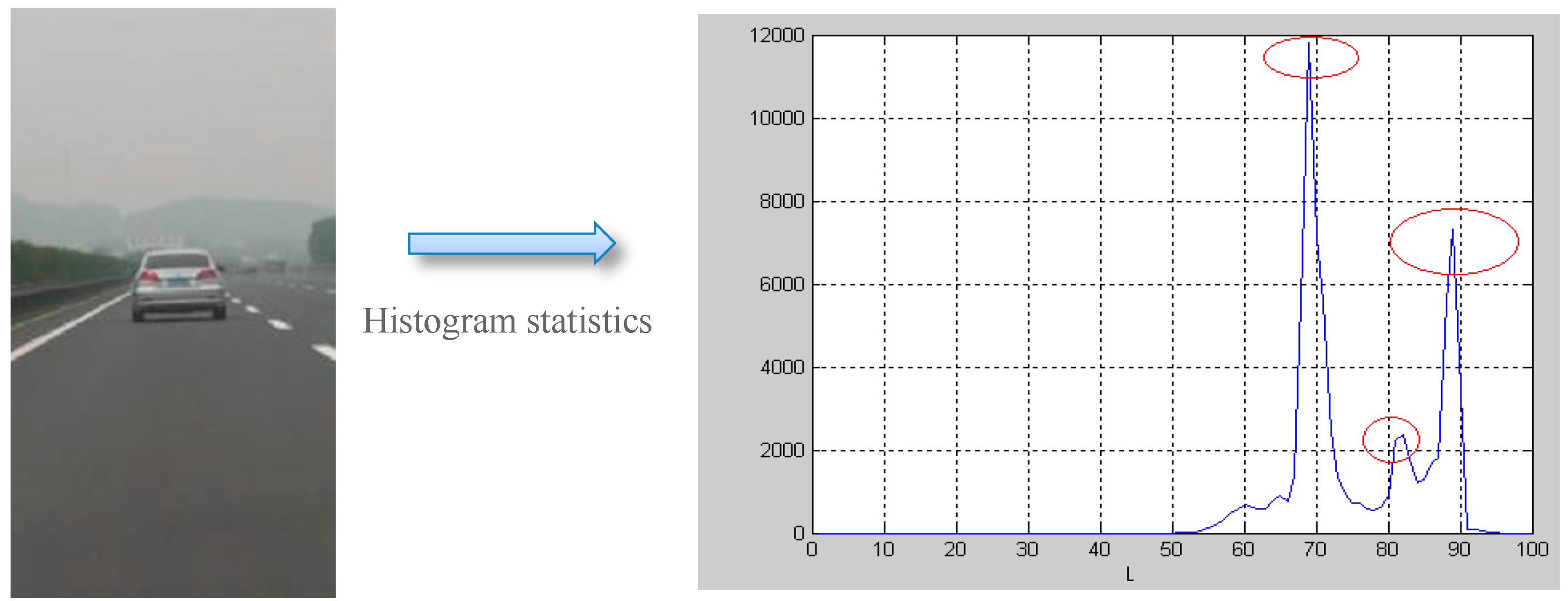
3.1.3. Hypothesis Generation: Shadow Detection

Vehicles may have many shapes and colors. One important feature in common is that they always cause shadow on the road surface. Vehicle candidates can be extracted by detecting the shadows underneath vehicles [18]. Potential shaded areas are the region with significant darker intensities than the road. In the ROI defined above, most of the impact of background is neglected and the darker area can be detected easily. Here, an adaptive K-Means algorithm for image segmentation is presented. The improvement of this method with traditional K-Means [21] is that the initial cluster centers and numbers are determined based on the histogram analysis.

Traditional K-Means algorithm has the advantages of being simple, easy to realize and stable, so it has become the most widely used method in research of cluster analysis. However, it is time-consuming and does not always guarantee unique clustering results. In this paper, we improved the algorithm in the following aspect. Instead of using random initialization, we follow a novel approach to provide initial cluster centers. Firstly, the histogram of L component in Lab color space is acquired, shown as Figure 6. It is clear that there are several peaks and valleys, and peaks always correspond with the maximum accumulation value of L component. Secondly, instead of providing random cluster centers, we choose the L value according to the peak as centers and the number of peaks as cluster numbers. According to Figure 6, there are three clusters with initial centers as 69, 82 and 89, respectively.

Figure 6. Histogram of L component.

Figure 6. Histogram of L component.

Table 2 shows the comparison results between two algorithms. It is indicated that the iteration and time-consumption are all improved greatly.

Table 2. Comparison of the different clustering algorithm.

	Traditional method				Improved method
Experiment No.	1	2	3	4	5
Iterations times	28	25	18	23	9
Time consuming (s)	1.9	1.7	1.3	1.5	0.15

Table 2. Comparison of the different clustering algorithm.

	Traditional method				Improved method
Experiment No.	1	2	3	4	5
Iterations times	28	25	18	23	9
Time consuming (s)	1.9	1.7	1.3	1.5	0.15

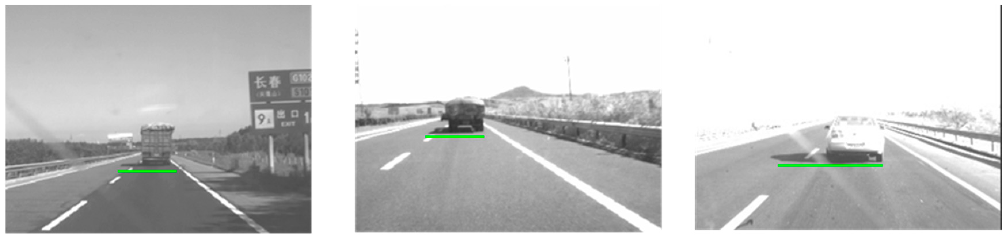
3.1.4. Hypothesis Generation: Extracting Bottom Lines for Vehicle Candidates

In real-driving environments, it is hard to obtain real bottom lines in the scenes with low sun, making vehicles cast long shadows, shown as Figure 7. This motivates us to solve it through other cues. Here, the vertical edges are in full used for refining the bottom lines detected with shadow information.

Figure 7. Vehicles cast long shadows in the scenes with low sun.

Figure 7. Vehicles cast long shadows in the scenes with low sun.

Firstly, in the ROI defined above, vertical edge points are obtained with Equation (2). Then, the edges are extracted with an improved line detection method based on HT. The improvement is that not only the edge but also the tip point of each line can be detected respectively. In order to obtain the tip point, the coordinates of each point used for HT are recorded in a link list while the parameters $(\rho ,\theta )$ are accumulated. With the proposed method, the vehicle vertical edge can be extracted accurately; examples are shown as Figure 8.

Figure 8. Examples for vertical edges detection.

Figure 8. Examples for vertical edges detection.

Based on the extracted vertical edge, the proposed method refines the left and right boundary on either side of the initial bottom line and finds the lowest tip points, respectively. Then, the length of initial bottom line is adjusted equal to the length between the lowest tip point in the left and right boundary. After adjusting, the length and vertical position of initial bottom lines that have an excessively short or long length are removed.

3.1.5. Hypothesis Generation: Extracting Bounding box for Vehicle Candidates

With above process, the bounding boxes for vehicle candidates are extracted easily. The left and right boundary of the boxes is set to the edges detected with refining method in Section 3.1.4. The height is set equal to the height of the left or right edge lines. In fact, in this paper, only the bottom is important for the following range estimation steps. However, the other boundaries of the box can provide cues for verification steps. Therefore, for convenience, only the bottom is shown in the real experiments.

3.2. Hypothesis Verification

In this step, the proposed method identifies a candidate using several features. Potential vehicles can be located using the method as discussed above. Once the bounding box corresponding to potential vehicle is defined, the verification search process is triggered.

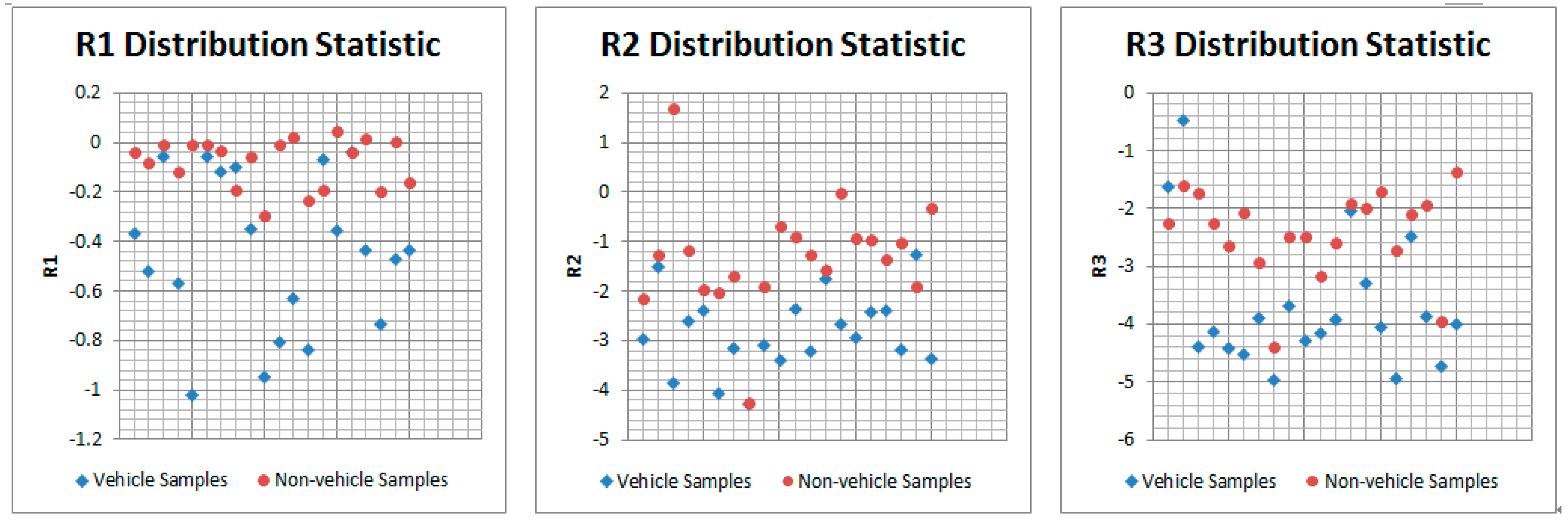
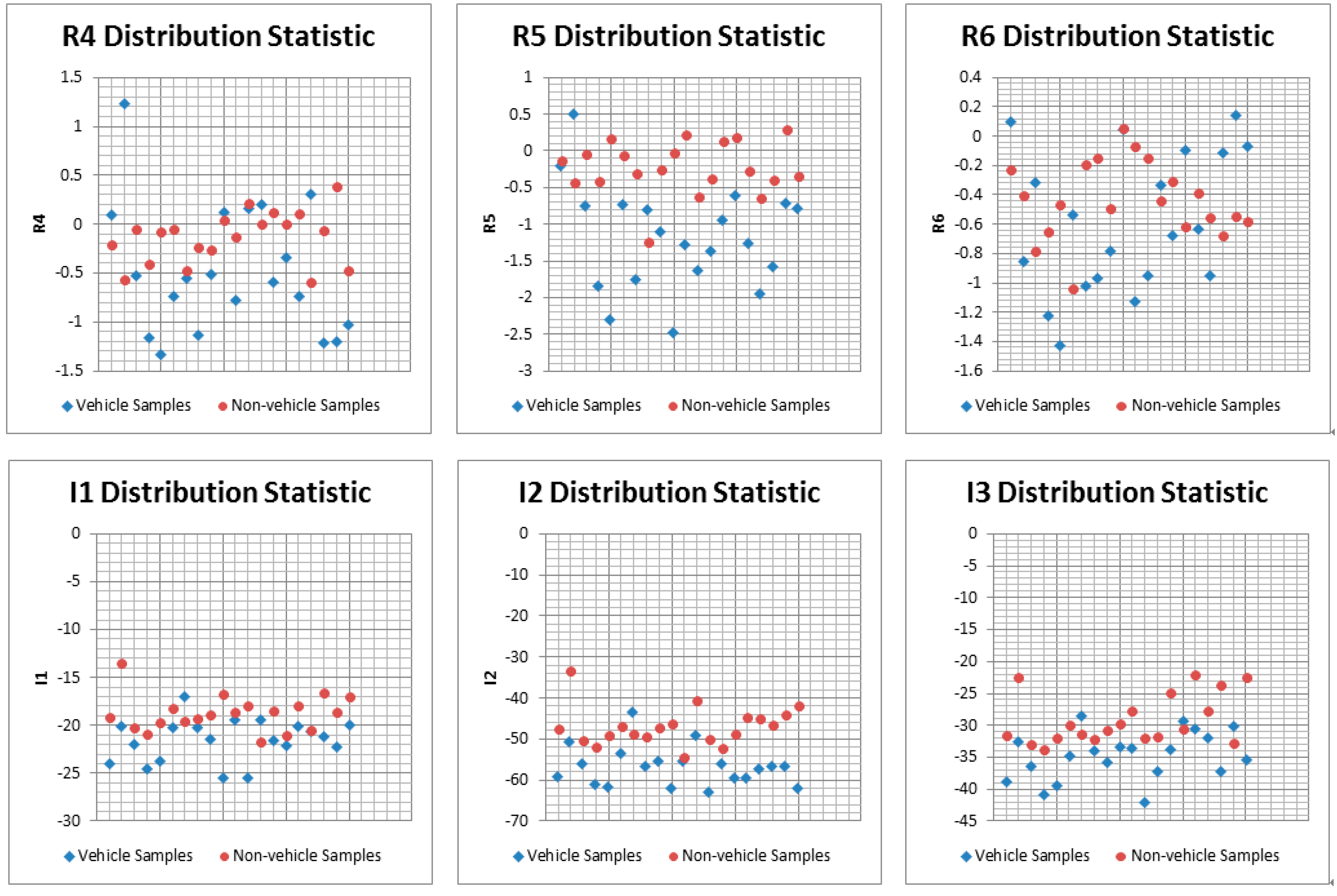
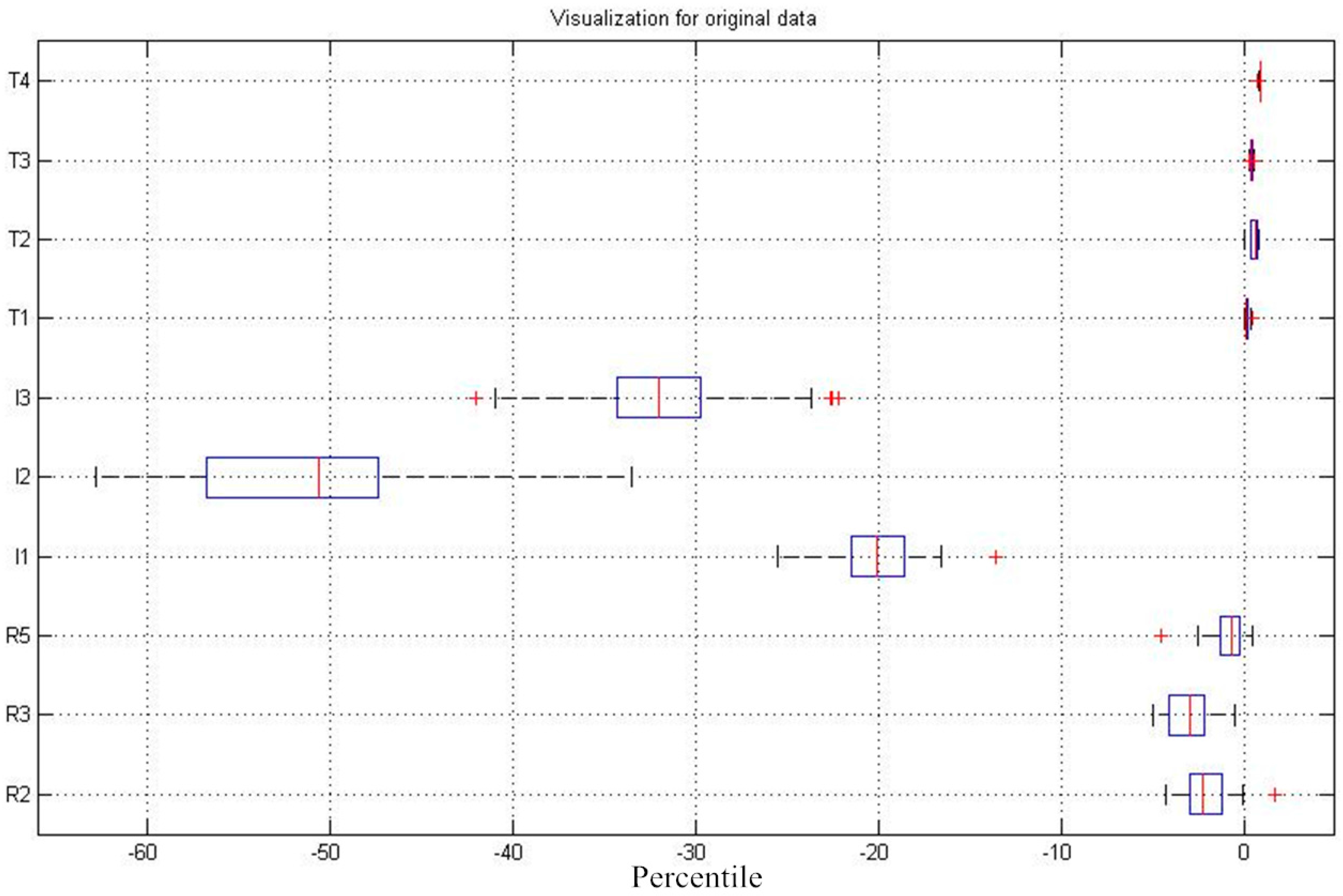
3.2.1. Hypothesis Verification: Features Extraction

Vehicles have many appearance features such as symmetry, rectangle, aspect ratio, textures etc. In this paper, a combined invariant feature named C-Moment is adopted. Furthermore, in order to reduce the influences caused by leaves, texture features are used for describing the shadow gray distribution properties underneath the vehicle.

(1) Composition of C-Moment features

Moments are designed to capture both global and detailed geometric information about the image. Hu [22,23] and affine invariant moment [24] are important features which are not sensitive to translation, stretch and rotation. In this paper, according to experimental results, the combined-moment invariants (including three improved Hu moments and three affine invariant moments) is designed for vehicle verification.

Figure 9 shows a statistic experiment for the extracted features R₁~R₅ and I₁~I₃. It indicates that the differences of R₂, R₃, R₅, I₁, I₂ and I₃ are obvious between vehicle and non-vehicle samples. Thus, they are considered as the most important features for identification. So, the combined features vector used for verification is defined as:

$$v={\left(R_2,R_3,R_5,I_1,I_2,I_3\right)}^T$$

(4)

Figure 9. Statistics of the moment with different samples.

Figure 9. Statistics of the moment with different samples.

(2) Texture features extraction

According to previous research, we found that some cases may lead to mistake recognition result only based on the shadows beneath the vehicle, especially in the real-driving environment with interference from shadow of the leaves, shown as Figure 10. Analysis indicates that there exist some similar properties between the shadows caused by vehicle and leaves, such as the dark intensity and edge gradient features. This is the main factor that leads to error. Therefore, this problem motivates us to solve it from the other aspects such as “target” internal texture characteristics. Considering time costs, texture feature extraction must be carried out in an area as small as possible. So, we extract the features in the bounding box for vehicle candidates described above.

Figure 10. Statistics of the moment with different samples.

Figure 10. Statistics of the moment with different samples.

Gray-level co-occurrence matrix (GLCM) is an important reflection of the changing rule of the image pixels on the directions and intervals. Previous research shows that there are 14 features obtained through GLCM which can be used for describing the image textures [25]. Of this, four features, including Energy (T₁), Contrast (T₂), Correlation (T₃) and Entropy (T₄), are uncorrelated and they can give out higher classification accuracy than the others. They are described as:

$$\{\begin{array}{ll}{f}_1={\displaystyle \sum _{i=0}^{L-1}{\displaystyle \sum _{j=0}^{L-1}{p}_d{(i,j)}^2}}& f_2={\displaystyle \sum _{n=0}^{L-1}{n}^2}\{{\displaystyle \sum _{i=0}^{L-1}{\displaystyle \sum _{j=0}^{L-1}{p}_d(i,j)}}\}\\ f_3=\frac{{\displaystyle \sum _{i=0}^{L-1}{\displaystyle \sum _{j=0}^{L-1}ij{p}_d(i,j)-{\mu }_1{\mu }_2}}}{{\sigma }_1^2{\sigma }_2^2}& f_4=-{\displaystyle \sum _{i=0}^{L-1}{\displaystyle \sum _{j=0}^{L-1}{p}_d(i,j)\log p_d(i,j)}}\end{array}$$

(5)

where, d represents the distance and direction between two pixels. L is the gray level of the image and i, j are the gray value of current pixels. So, $p_d(i,j)$ reflects a probability that, along the given spatial location relationship d (distance and direction), one pixel with gray value i reaches to the pixel with gray value j.

In order to verify the validity of texture features used for classifying the shadows caused by vehicle and leaves, experiment about f₁~f₄ is conducted, which is shown as Figure 11. From the statistical results, some cues can be inferred. Firstly, the property distribution of leaves shadows shows that there are some convergences within the four features, especially in the contrast, correlation and homogeneity. Secondly, the property of vehicle shadow shows a certain dispersion property besides the homogeneity distribution. However, in respective statistical figures, the differences between vehicle and leaves shadow are obvious and can be classified with certain methods. Therefore, these texture features can be considered as important cues for identifying the shadows from the vehicles or leaves.

Figure 11. Texture property distribution statistics.

Figure 11. Texture property distribution statistics.

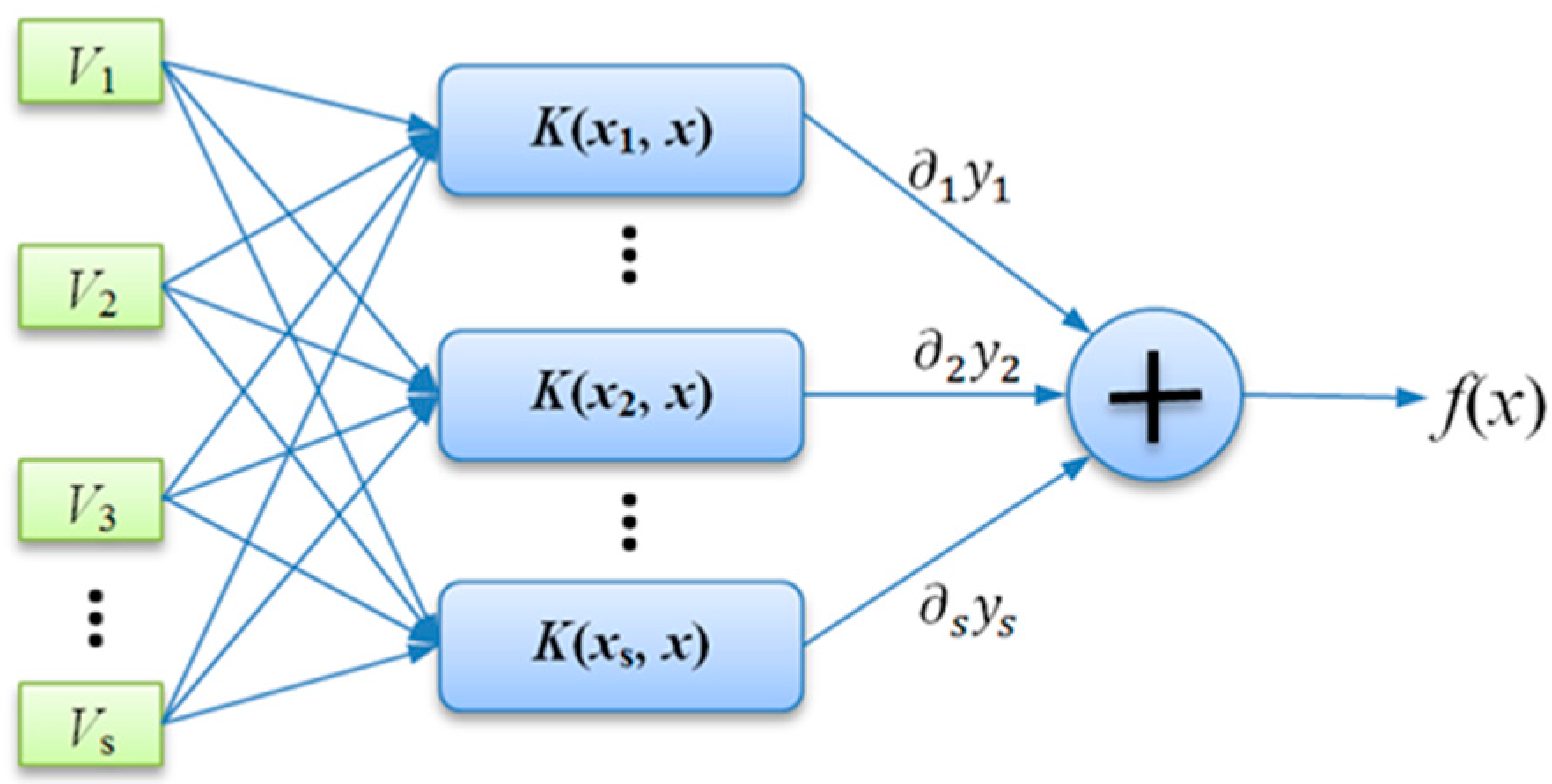
3.2.2. Hypothesis Verification: Vehicle Candidate Verification by SVM

As a new and promising technique for classification problem tools, SVM has been successfully applied widely since its introduction [26]. In real applications, the parameters need to be optimized which greatly impacts the performance of SVMs. Improper selection of the parameters could cause either the over-fitting or under-fitting of the training data points. These parameters mainly include the penalty factor C and the parameters of kernel function (for instance, parameter γ of RBF kernel function). At present, grid search algorithm [27] is the most reliable method for the off-line data training process. However, for large scale or real-time feature practice application, the considerable searching time cannot be accepted. Therefore, many studies have been devoted to improving the efficiency of the parameter optimization in SVM by using heuristic algorithms.

This paper aims to build a hybrid model for vehicle candidate verification, which is named the SVM-GA model. The architecture of the solution consists of three modules: PCA unit, SVM unit and GA unit. The hybrid model can be described as in Figure 12.

Figure 12. Flow-chart of the hybrid model.

Figure 12. Flow-chart of the hybrid model.

(1) Support vector classification

The training procedure of SVM is finding the hyper-plane which optimally separates two classes with maximum margin. Given a training set of instance-label pairs (x_i, y_i); i = 1, …, l, where x_i∈Rⁿ and y∈l, the SVM requires solution of the following optimization problem:

$$\begin{array}{l}\underset{\omega ,b,\xi }{\min }\begin{array}{cc}& \frac{1}{2}\end{array}{w}^T\cdot w+C{\displaystyle \sum _{i=1}^l{\xi }_i}\\ s.t.\begin{array}{cc}& y_i[w^T\cdot \phi (x_i)+b]\end{array}\ge 1-{\xi }_i\\ {\xi }_i\ge 0,i=1,2,\cdots ,l\end{array}$$

(6)

where training vectors x_i is mapped into a higher (maybe infinite) dimensional space by the kernel function Φ. SVM finds a linear separating hyper plane with the maximal margin in this higher dimensional space. C > 0 is the penalty parameter of error term.

The dual optimization problem is obtained with Lagrange multiplier ${\partial }_i$, shown as following:

$$\begin{array}{ll}\underset{\partial }{\max }& W={\displaystyle \sum _{i=1}^l{\partial }_i}-\frac{1}{2}{\displaystyle \sum _{i=1}^l{\displaystyle \sum _{i=1}^l{\partial }_i{\partial }_j{y}_i{y}_{j}K(x_i,x_j)}}\\ s.t.& {\displaystyle \sum _{i=1}^l{\partial }_i{y}_i=0},0\le {\partial }_i\le C,i=1,2,\cdots ,l\end{array}$$

(7)

Then, the SVM decision function is:

$$f(x)=\mathrm{sgn}({\displaystyle \sum _{i=1}^l{\partial }_{i}k(x_i,x)+b})$$

(8)

In this paper, the SVM model constructed will be trained with 10 related features demonstrated above and then it will be used to recognize the vehicles with the validation dataset. The structure of the SVM model is shown as Figure 13.

Figure 13. Flow-chart of the hybrid model.

Figure 13. Flow-chart of the hybrid model.

(2) GA for parameters optimization

Although SVM is feasible and applicable for vehicle candidate verification, there are some parameters, which greatly impact the performance of SVMs, that need to be optimized. In general, for the RBF kernel, as a nonlinearly kernel function, the parameters such as $C, \gamma and \epsilon$ are the key elements and they directly determine the prediction performance of SVM. Thus, the parameter optimization is important for improving the prediction accuracy. In this paper, a genetic algothrim is used for finding the best parameters for the presented SVM model. In general, the process of GA can be briefly described as follows:

• Encoding of chromosome: In GA, a standard representation of each candidate solution is as a chromosome that is composed of “genes”. For the SVM parameters optimization problem in this paper, the real encodings were adopted since the parameters $C, \gamma and \epsilon$ are continuous-valued. Each chromosome consists of $gen{e}_1^g$, $gen{e}_2^g$ and $gen{e}_3^g$, which represent the three parameters, respectively. Here, g is the current generation. In order to reduce the search space, the previous literature has given out the recommended searching space which respectively attribute to the range $C\in \left[2^{-5},2^5\right]$, $\epsilon \in \left[2^{-13},2^{-1}\right]$ and $\gamma \in \left[0,2\right]$.
• Fitness function: A fitness function is a particular type of objective function that is used to summarise how close the possible solution is to achieving the set aims. For the SVM parameters optimization problem in this paper, considering that GA is always finding the maximum fitness of the individual chromosome, mean squared error (MSE) is adopted.

  $$fitness=\frac{1}{l}{\displaystyle \sum }_{i=1}^l{\left(f\left(x_i\right)-y_i\right)}^2$$

  (9)

  where, $f\left(x_i\right)$ is the prediction value by the SVM model; $y_i$ is the observed value; $l$ is the number of observation variables.
• Selection operation: During each successive generation, a proportion of the existing population is selected to breed a new generation. Individual solutions are selected through a fitness-based process, where fitter solutions (as measured by a fitness function) are typically more likely to be selected. In this paper, the roulette selection strategy is adopted. Based on the fitness calculation results, the sum fitness value of the entire population and then the ratio corresponding to each chromosome are obtained. In the next step, a random number (range from 0 to 1) is used for determining the range of the cumulative probability. The chromosome falling within the expected range is selected out.
• Genetic operators: For each new solution to be produced, a pair of “parent” solutions is selected for breeding from the pool selected previously. A second generation population of solutions is generated from those selected through a combination of genetic operators: crossover (also called recombination), and mutation. Crossover is a genetic operator used to vary the programming of a chromosome or chromosomes from one generation to the next. It is analogous to reproduction and biological crossover. Cross over is a process of taking more than one parent solution and producing a child solution from them. In literature [28], an arithmetic crossover operator is used.

  $$\begin{array}{c}ge{n}_{k,I}^t={\alpha }_{i}ge{n}_{k,I}^{t-1}+\left(1-{\alpha }_i\right)ge{n}_{k,II}^{t-1}\\ ge{n}_{k,II}^t={\alpha }_{i}ge{n}_{k,II}^{t-1}+\left(1-{\alpha }_i\right)ge{n}_{k,I}^{t-1}\end{array}$$

  (10)

  where, $ge{n}_k^{t-1}$ is the “parent” chromosomes; $ge{n}_k^t$ is the “child” chromosomes; ${\alpha }_i$ is a random probability value with range (0,1).
  Mutation is a genetic operator used to maintain genetic diversity from one generation chromosome to the next. Mutation occurs during evolution according to a user-definable mutation probability. A very small mutation rate may lead to premature convergence of the genetic algorithm and a very high rate may lead to loss of good solutions unless there is elitist selection. In general, the mutation rate is defined with the range [0.001, 0.1]. In this paper, according to the previous literature, the mutation rate is set to 0.05.
• Termination: This generational process is repeated until a termination condition has been reached. In this paper, the search loop continues until $MS{E}_n-MS{E}_{n-1}<0.0001$ or the number of generation reaches the maximum number of generations $T_{max}$.

(3) PCA for reducing the dimensionality of input data sets

In order to speed the velocity of SVM training and prediction with maintaining the main information of samples and not changing the distribution characteristics, in this paper, PCA method is used before the variables is input into the SVM model for training and prediction. In PCA, which kind of data is used will has a great influence for the result of the analysis. Existing literature shows that the analysis results are different when the covariance matrix and the correlation matrix are used for PCA, respectively. In this paper, the various features variables can reflect the vehicle candidate from different aspects. Thus, there exists some relevance between the variables. Meanwhile, the dimensional of each variable is different. Therefore, based on the above analysis, we consider using the correlation matrix for the subsequent PCA process.

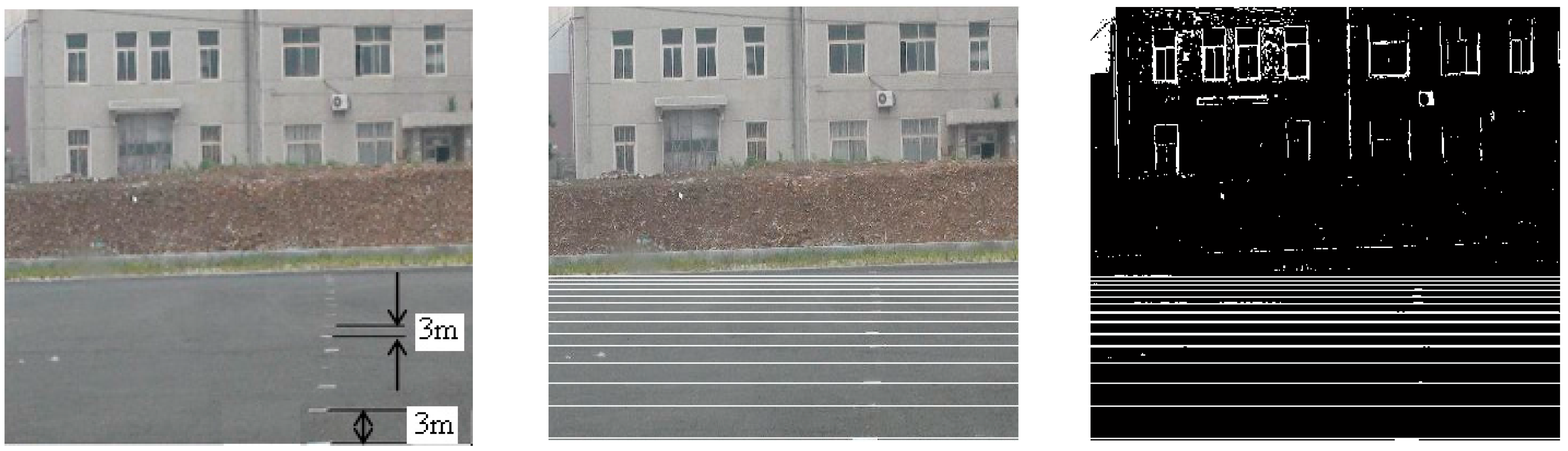
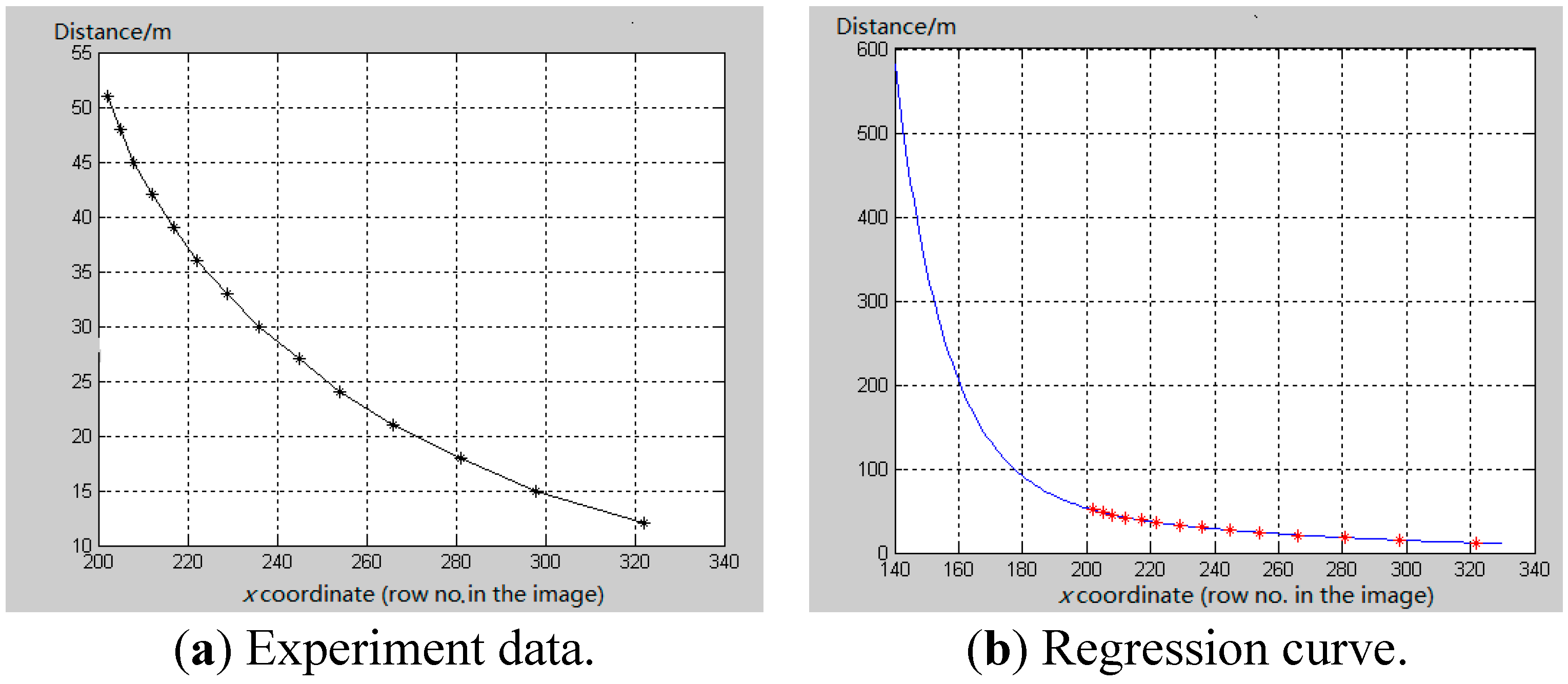
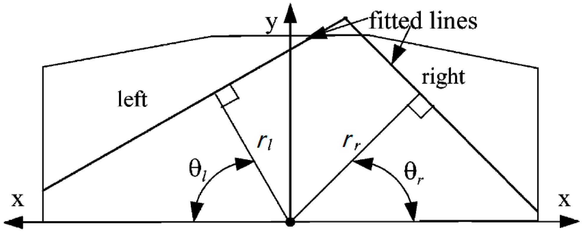
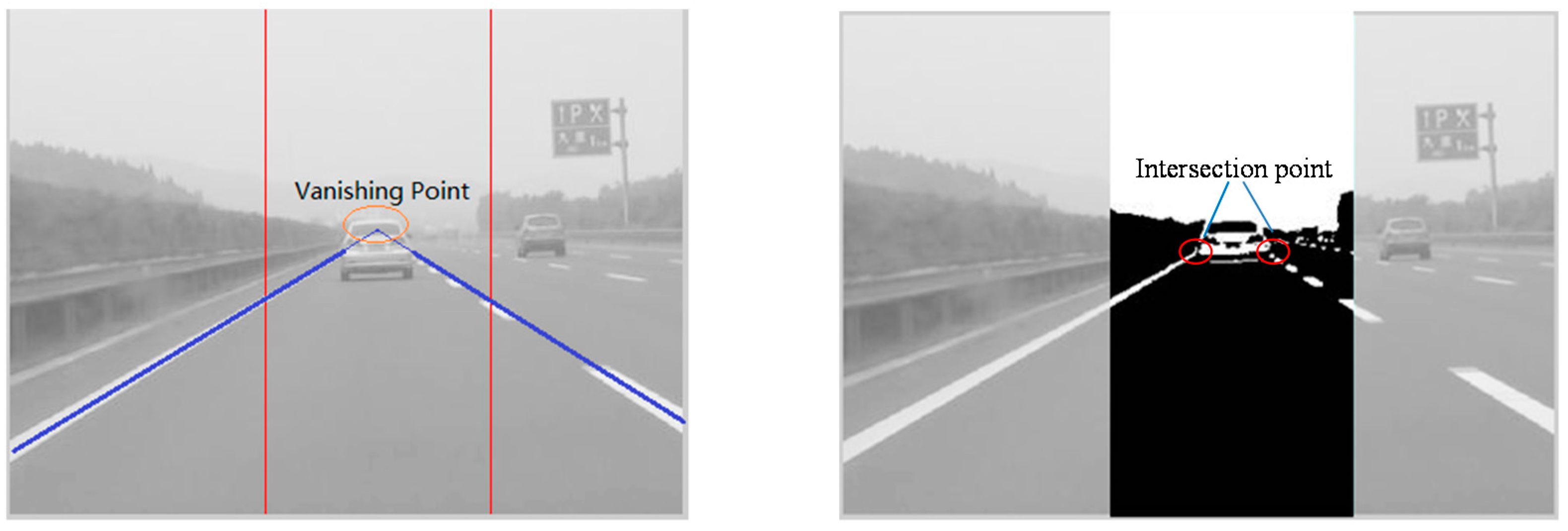
4. Range Estimation

Once the forward vehicle is detected, the system will start to estimate the distance from the vehicle to host vehicle. In this paper, we establish a distance estimation model based on the assumption that road surface is similar to a plane. The parameters of the model can be recognized through off-line calibration with regression analysis. The position of the bottom line detected taking the above steps is utilized to estimate the longitudinal distance to the preceding vehicle. Within the calibration, firstly a calibration scene is established with some control points (shown as Figure 14). In which, the distance between each point and the mounted camera is known in advance. Once the position of the control points in the image is obtained, then the perspective projection model can be established through data regression analysis.

Figure 14. Calibration process of the range estimation model.

Figure 14. Calibration process of the range estimation model.

In the calibration step, the interval distance between each control points is 3 m and the distance from control point to camera can be inferred respectively. According to the binary image, the horizontal line which control point belongs to is detected with image processing. Therefore, the control point coordination in the image can be obtained and the perspective projection can be calculated through regression analysis. Figure 15 is the regression result for range estimation. The accurate mathematic model of the curve is $y=a{e}^{(bx)}+c{e}^{(dx)}$, in which vector ${[a,b,c,d]}^T$ for this model is ${[\text{3}.\text{59}\times {10}^6\text{, }-0.0\text{6337, 336}.\text{3, }-0.0\text{1}0\text{42}]}^T$ and the root mean square error is 0.206.

Figure 15. The range estimation regression analysis.

Figure 15. The range estimation regression analysis.

Based on the established range estimation model, the distance to the forward vehicle can be achieved. Part of the verification samples can be found in the Experimental Section.

5. Experimental Results

Based on the above proposed model, in this section, the evaluation results are presented.

5.1. Performance Evaluation of Improved SVM

In order to measure performance of the presented method on real-world data, 160 samples (including 80 positive and 80 negative samples) from real-driving environment are selected. At first, each sample is grouped according to their type (positive or negative), respectively. Then, the feature vectors $v_i={\left(R_2,R_3,R_5,I_1,I_2,I_3,T_1,T_2,T_3,T_4\right)}^T$ corresponding to each samples is calculated. Figure 16 is the features distribution statistical result with boxplot method. It can be seen that most of the samples fall within the range between the 25th and 75th percentile. Several outlier points correspond to each negative sample. Furthermore, for the purpose of testing the performance of the proposed SVM model with optimized parameters, the dataset is divided into two subsets, 80% of the samples are used for training and 20% for testing.

Figure 16. Calibration process of the range estimation model.

Figure 16. Calibration process of the range estimation model.

During the SVM model training process, the parameters selection, mainly including penalty factor c and g of kernel function, greatly impacts the performance of SVM classification, which needs to be optimized and set by users. To properly optimize the parameters, based on the proposed SVM-GA model in Section 3.2.2, tests were conducted on the sample data respectively. The results are shown as Figure 17 and detailed information is listed in Table 3. In which, CG-SVM refers to that parameters are optimized with the cross grid searching method, GA-SVM refers to gene algorithm searching method and PSO-SVM refers to the particle swarm optimization method.

Figure 17. Parameter search with different optimization methods.

Figure 17. Parameter search with different optimization methods.

Based on the above analysis results, it is indicated that the accuracies of GA and PSO methods are very close to that of the CG method which is a common algorithm used for SVM parameter searches. However, on the contrary, the time cost is significantly different for the SVM model’s parameter optimization. There are great advantages in the GA-SVM method for improving calculation speed. In addition, the number of support vectors is tremendously different between CG, GA and PSO search methods. The GA method can achieve the same classification performance with the traditional CG method as well as enhance the operation speed of the algorithm greatly.

Table 3. Comparison with different parameter search results.

Method	Best c	Best g	Accuracy		Testing time	Tmax	SVTotal
			Train	Test
CG-SVM	9.1896	0.1088	99.22%	96.8%	5.3 ms	--	16
GA-SVM	4.0338	0.1859	99.22%	96.8%	0.42 ms	50	19
PSO-SVM	0.1	2.2778	98.44%	96.8%	2.47 ms	50	71

Table 3. Comparison with different parameter search results.

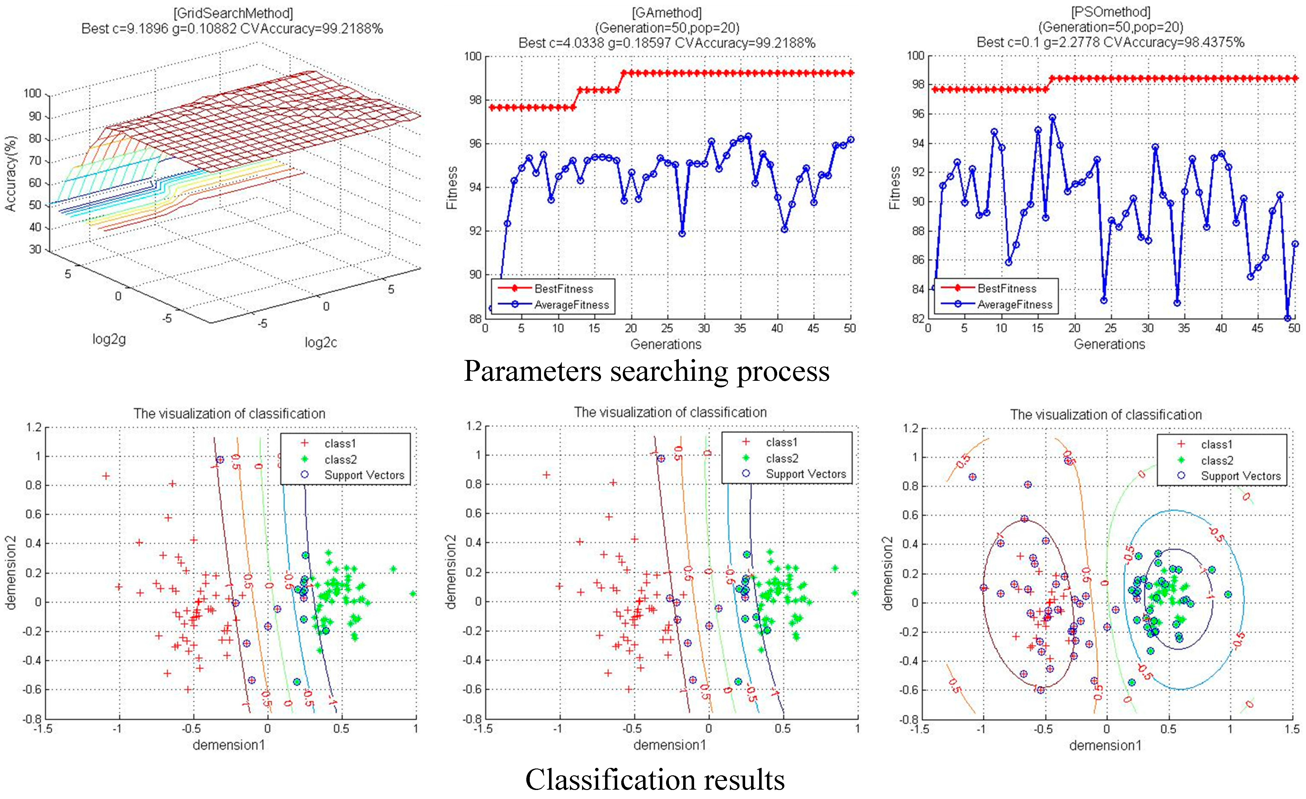
Method	Best c	Best g	Accuracy		Testing time	Tmax	SVTotal
			Train	Test
CG-SVM	9.1896	0.1088	99.22%	96.8%	5.3 ms	--	16
GA-SVM	4.0338	0.1859	99.22%	96.8%	0.42 ms	50	19
PSO-SVM	0.1	2.2778	98.44%	96.8%	2.47 ms	50	71

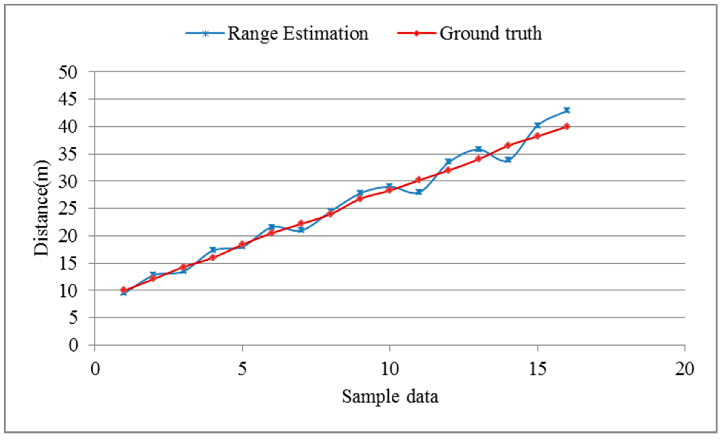
5.2. Performance Evaluation of Range Estimation

Before testing on the public road, the proposed range estimation method was tested on the proving ground. The longitudinal distance was measured by way of changing the relative position between the host and target vehicle. The platform for the range estimation test is shown as Figure 18. In which, the ground truth distance was obtained through the LIDAR sensor (SICK LMS-211) mounted on the front bumper of the host vehicle and the estimation distance was achieved with the proposed model discussed above. Figure 19 shows the result of range estimation.

Figure 18. Platform for range estimation test.

Figure 18. Platform for range estimation test.

Figure 19. Range estimation results on the proving ground.

Figure 19. Range estimation results on the proving ground.

From the test results in Figure 19, some cues can be inferred. Firstly, the absolute error increased with the distance extended. It can be explained in such a way that during the establishment of the range estimation model, the farther control points are presented in the image with lower resolution, shown as Figure 14. So, the precision of the established model depends closely on the distribution of the control points. Secondly, analysis result shows that the average range error is 5.18%. This level of precision is enough for a driver assistance system in practical applications.

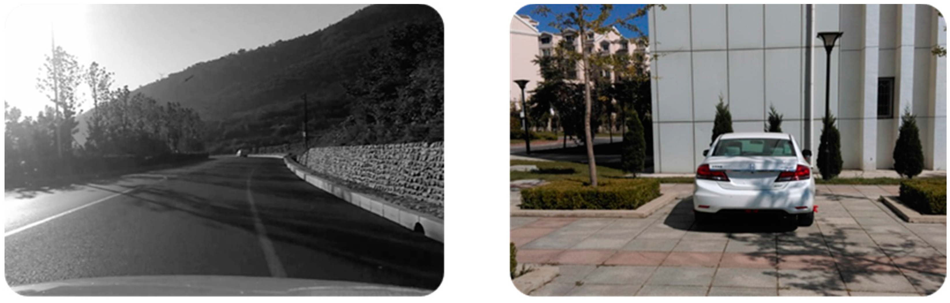
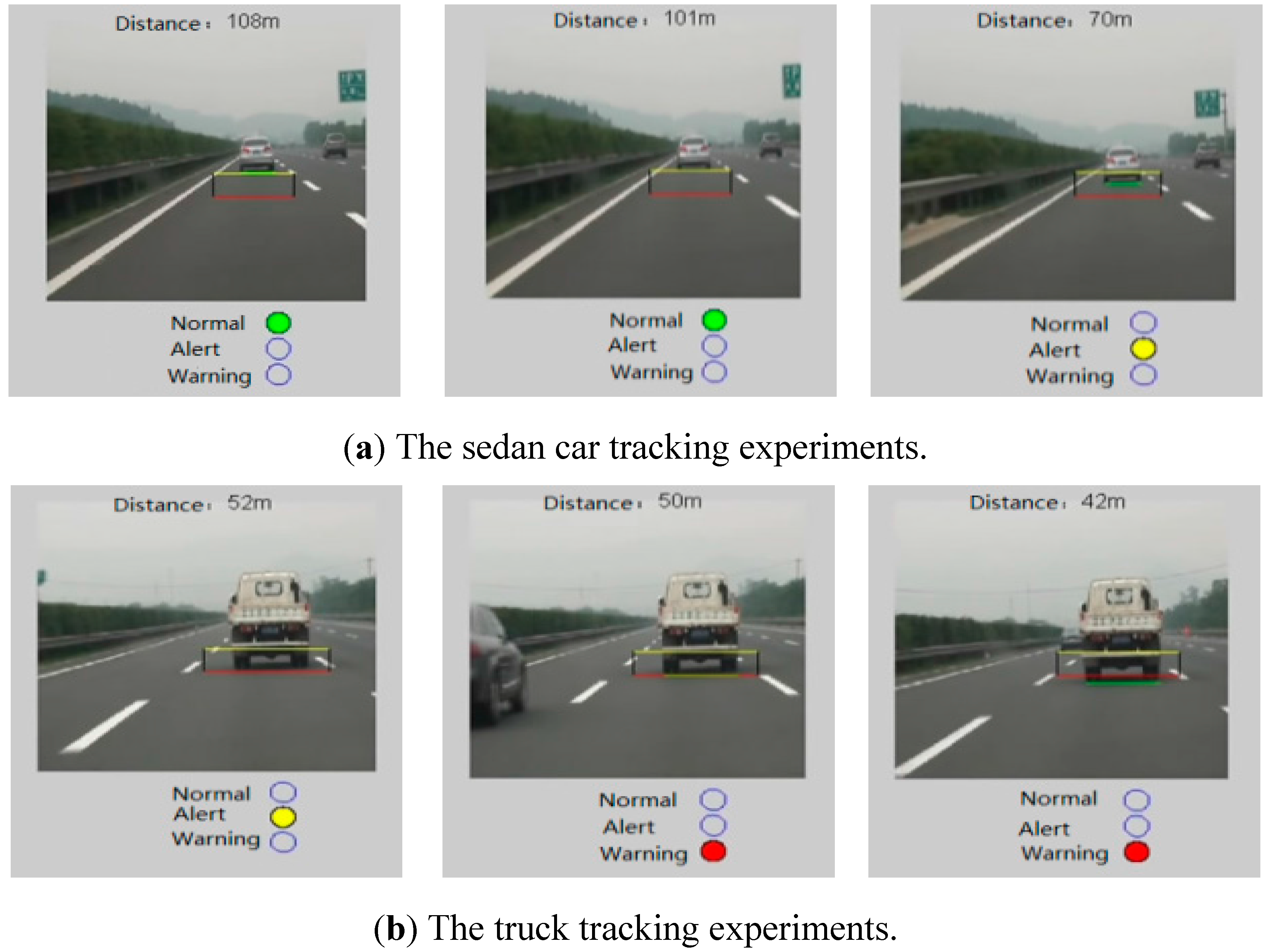
5.3. Model Verification in a Real-Driving Environment

In this section, the test results in a real driving environment are presented. The proposed system was implemented on a vehicle-mounted computer platform (1600 MHz, 512 RAM) with a few peripheral devices such as LCD screen and USB etc. An AVT camera was connected to the platform with a USB interface and mounted in the front windshield of the host car to acquire an image with resolution 320 × 240 at 100 fps. The experiment was conducted on the Highway G15 in China (shown as Figure 20) from Dalian to Bayuquan, in the daytime with various environments such as sunlit and rainy. The public roads where the test vehicle is driven included cluttered backgrounds, such as trees and poorly illuminated places.

Figure 20. Experiment site of Dalian-Bayuquan district.

Figure 20. Experiment site of Dalian-Bayuquan district.

During the experiment, vehicles including sedan, minivan, and truck are tested. Based on the experiment analysis, the results show that the average vehicle detection rate is above 95%. Detailed information about the experiment is listed in Table 4.

Table 4. Detection results on the public roads.

Weather	Sunlit			Rainy
Vehicle type	Sedan	Minivan	Truck	Sedan	Minivan	Truck
# of sampled frame	1450	1080	1260	1150	980	1100
# of detection	1408	1030	1190	1108	949	1020
# of false positive	72	65	58	35	27	52
Detection rate (%)	97.1	95.37	94.44	96.34	96.83	92.73

Table 4. Detection results on the public roads.

Weather	Sunlit			Rainy
Vehicle type	Sedan	Minivan	Truck	Sedan	Minivan	Truck
# of sampled frame	1450	1080	1260	1150	980	1100
# of detection	1408	1030	1190	1108	949	1020
# of false positive	72	65	58	35	27	52
Detection rate (%)	97.1	95.37	94.44	96.34	96.83	92.73

During the entire experiment, the proposed method was processed fast enough for FCWS. The minimum processing time (tracking mode) is 20 ms/frame, the maximum processing time is 35 ms/frame, and the average processing time is 26.3 ms/frame. Therefore, it is indicated that the proposed method has a good reliability with low cost computation and strong potential effectiveness to be applied to the driver assistance system. Figure 21 presents the detection results for various kinds of interference. In which, the indicating lamp is set with different colors according to the distance estimated through the system model. When the distance was less than the default threshold, then the lamp was set with green, yellow or red color, respectively, according to different warning levels. During the experiment, the detected “target” (sedan, truck or minivan) footprint was distinguished by a green line and the alert, warning threshold was shown with yellow and red lines in order to display the warning results.

Figure 21. Partial tracking result with different interference.

Figure 21. Partial tracking result with different interference.

6. Conclusion and Perspective

A camera-based forward vehicle detection method is proposed in this paper. As such, the road scene is acquired with a color camera, and the vehicle candidate is extracted using the shadow underneath the vehicle. In order to reduce the interference of the leaves’ shadow, texture features of the shadow are used for shadow recognition cues. In verification steps, various features consisting of three Hu moments, three affine invariant moments and four texture features are fused with an improved SVM model. The system also provides distance information in order to provide a safe range warning. Finally, the proposed method is successfully implemented on a test car and tested on Highway G15 in China, and its effectiveness is verified. Experimental results show the reliability in terms of both detection rate and potential effectiveness when applied in a real-driving environment.

Since in the real-driving environment there are so many affecting factors for vehicle detection, for further studies, more environmental factors such as night driving must be considered to optimize system performance and make the system more robust.

References

- Dagan, E.; Mano, O.; Stein, G.P.; Shashua, A. Forward collision warning with a single camera. In Proceedings of the 2004 IEEE Intelligent Vehicles Symposium, Parma, Italy, 14–17 June 2004; pp. 37–42.
- Park, S.J.; Kim, T.Y.; Kang, S.M.; Koo, K.H. A novel signal processing technique for vehicle detection radar. In Proceedings of the 2003 IEEE MTT-S International Microwave Symposium Digest, Philadelphia, PA, USA, 8–13 June 2003; Vol. 601, pp. 607–610.
- Wang, C.C.; Thorpe, C.; Suppe, A. Ladar-based detection and tracking of moving objects from a ground vehicle at high speeds. In Proceedings of the 2003 IEEE Intelligent Vehicles Symposium, Columbus, OH, USA, 9–11 June 2003; pp. 416–421.
- Baek, Y.M.; Kim, W.Y. Forward vehicle detection using cluster-based adaboost. Opt. Eng. 2014, 53. [Google Scholar] [CrossRef]
- Zhan, W.; Ji, X. Algorithm research on moving vehicles detection. Procedia Eng. 2011, 15, 5483–5487. [Google Scholar] [CrossRef]
- Aytekin, B.; Altug, E. Increasing driving safety with a multiple vehicle detection and tracking system using ongoing vehicle shadow information. In Proceedings of the 2010 IEEE International Conference on Systems Man and Cybernetics (SMC), Istanbul, Turkey, 10–13 October 2010; pp. 3650–3656.
- Sivaraman, S.; Trivedi, M.M. Looking at vehicles on the road: A survey of vision-based vehicle detection, tracking, and behavior analysis. IEEE Trans. Intell. Transp. Syst. 2013, 14, 1773–1795. [Google Scholar] [CrossRef]
- Ming, Q.; Jo, K.-H. Vehicle detection using tail light segmentation. In Proceeding of the 6th International Forum on Strategic Technology (IFOST), Harbin, China, 22–24 August 2011; pp. 729–732.
- O’Malley, R.; Jones, E.; Glavin, M. Rear-lamp vehicle detection and tracking in low-exposure color video for night conditions. IEEE Trans. Intell. Transp. Syst. 2010, 11, 453–462. [Google Scholar] [CrossRef]
- Mithun, N.C.; Rashid, N.U.; Rahman, S.M.M. Detection and classification of vehicles from video using multiple time-spatial images. IEEE Trans. Intell. Transp. Syst. 2012, 13, 1215–1225. [Google Scholar] [CrossRef]
- Zhang, Y.; Wang, X.; Qu, B. Three-frame difference algorithm research based on mathematical morphology. Procedia Eng. 2012, 29, 2705–2709. [Google Scholar] [CrossRef]
- Mandellos, N.A.; Keramitsoglou, I.; Kiranoudis, C.T. A background subtraction algorithm for detecting and tracking vehicles. Expert Syst. Appl. 2011, 38, 1619–1631. [Google Scholar] [CrossRef]
- Vapnik, V.N. An overview of statistical learning theory. IEEE Trans. Neural Netw. 1999, 10, 988–999. [Google Scholar] [CrossRef] [PubMed]
- Yao, B.; Yao, J.; Zhang, M.; Yu, L. Improved support vector machine regression in multi-step-ahead prediction for rock displacement surrounding a tunnel. Sci. Iran. 2014, 21, 1309–1316. [Google Scholar]
- Yao, B.; Yu, B.; Hu, P.; Gao, J.; Zhang, M. An improved particle swarm optimization for carton heterogeneous vehicle routing problem with a collection depot. Ann. Oper. Res. 2015. [Google Scholar] [CrossRef]
- Cao, L.J.; Tay, F.E.H. Support vector machine with adaptive parameters in financial time series forecasting. IEEE Trans. Neural Netw. 2003, 14, 1506–1518. [Google Scholar] [CrossRef] [PubMed]
- Yao, B.; Hu, P.; Zhang, M.; Jin, M. A support vector machine with the tabu search algorithm for freeway incident detection. Int. J. Appl. Math. Comput. Sci. 2014, 24, 397–404. [Google Scholar] [CrossRef]
- Liu, W.; Wen, X.; Duan, B.; Yuan, H.; Wang, N. Rear vehicle detection and tracking for lane change assist. In Proceedings of the 2007 IEEE Intelligent Vehicles Symposium, Istanbul, Turkey, 13–15 June 2007; pp. 252–257.
- Chen, Q.; Zhao, L.; Lu, J.; Kuang, G.; Wang, N.; Jiang, Y. Modified two-dimensional otsu image segmentation algorithm and fast realisation. IET Image Process. 2012, 6, 426–433. [Google Scholar] [CrossRef]
- Yang, X.; Duan, J.; Gao, D.; Zheng, B. Research on lane detection based on improved hough transform. Comput. Meas. Control 2010, 18, 292–295. [Google Scholar]
- MacQueen, J. Some methods for classification and analysis of multivariate observations. In Proc. of the fifth Berkeley Symposium on Mathematical Statistics and Probability; Le Cam, L.M., Neyman, J., Eds.; University of California Press: Berkeley, CA, USA, 1976; pp. 281–297. [Google Scholar]
- Hu, M.-K. Visual pattern recognition by moment invariants. IRE Trans. Inf. Theory 1962, 8, 179–187. [Google Scholar]
- Han, B.; Xu, Z.; Wang, S. Scale invariance of discrete moment. J. Data Acquis. Process. 2008, 23, 555–558. [Google Scholar]
- Flusser, J.; Suk, T. Affine moment invariants: A new tool for character recognition. Pattern Recog. Lett. 1994, 15, 433–436. [Google Scholar] [CrossRef]
- Mridula, J.; Kumar, K.; Patra, D. Combining glcm features and markov random field model for colour textured image segmentation. In Proceedings of the 2011 International Conference on Devices and Communications (ICDeCom), Mesra, India, 24–25 February 2011; pp. 1–5.
- Cortes, C.; Vapnik, V. Support-vector networks. Mach. Learn. 1995, 20, 273–297. [Google Scholar] [CrossRef]
- Hsu, C.-W.; Chang, C.-C.; Lin, C.-J. A Practical Guide to Support Vector Classication; National Taiwan University: Taipei, Taiwan, 2003. [Google Scholar]
- Yu, B.; Yang, Z.; Cheng, C. Optimizing the distribution of shopping centers with parallel genetic algorithm. Eng. Appl. Artif. Intell. 2007, 20, 215–223. [Google Scholar] [CrossRef]
© 2015 by the authors; licensee MDPI, Basel, Switzerland. This article is an open access article distributed under the terms and conditions of the Creative Commons Attribution license (http://creativecommons.org/licenses/by/4.0/).
Share and Cite
Gang, L.; Zhang, M.; Zhao, X.; Wang, S. Improved Genetic Algorithm Optimization for Forward Vehicle Detection Problems. Information 2015, 6, 339-360. https://doi.org/10.3390/info6030339
Gang L, Zhang M, Zhao X, Wang S. Improved Genetic Algorithm Optimization for Forward Vehicle Detection Problems. Information. 2015; 6(3):339-360. https://doi.org/10.3390/info6030339
Chicago/Turabian StyleGang, Longhui, Mingheng Zhang, Xiudong Zhao, and Shuai Wang. 2015. "Improved Genetic Algorithm Optimization for Forward Vehicle Detection Problems" Information 6, no. 3: 339-360. https://doi.org/10.3390/info6030339
APA StyleGang, L., Zhang, M., Zhao, X., & Wang, S. (2015). Improved Genetic Algorithm Optimization for Forward Vehicle Detection Problems. Information, 6(3), 339-360. https://doi.org/10.3390/info6030339