A Multi-View Projection and 3D Feature Fusion Model for Full-Reference Point Cloud Quality Assessment

Abstract

Point clouds are widely used to represent 3D visual content in immersive media, digital twins, and autonomous systems, but acquisition, compression, transmission, and rendering can introduce visible geometry and attribute distortions. Full-reference point cloud quality assessment (FR-PCQA) aims to predict the perceptual quality of a distorted point cloud by comparing it with a reference. A reliable FR-PCQA model should consider both the perception of 3D content by the human visual system via projected views and the manifestation of quality degradation in the point cloud geometry, color, and spatial structure. In this paper, we propose a multi-view projection and 3D feature fusion model for FR-PCQA. The proposed model integrates two complementary branches. In the projection branch, DISTS is applied to multi-view renderings aligned with the reference to capture perceptual similarity, and an additional six groups of geometric and photometric fidelity features (e.g., occupancy, depth fidelity and gradient domain fidelity) are developed to describe explicit geometric and photometric differences in the projected observations. In the 3D Feature Fusion branch, PCQM measures local geometry and color degradation, while a global structural descriptor with eight groups covering point count, position, scale, spatial distribution, and density is constructed to characterize the global properties of point clouds. Finally, a gradient boosting regression tree (GBRT) regressor is employed to predict the final quality score. Extensive experimental results show that the Spearman rank order correlation coefficient (SROCC) values are 0.91537, 0.9101, and 0.9778 on the SJTU-PCQA, WPC, and ICIP2020 datasets, respectively, outperforming the existing PCQA methods. These results indicate that the proposed multi-view projection and 3D feature fusion model provides an accurate and interpretable solution for FR-PCQA.

1. Introduction

With the rapid development of immersive media, digital twins, autonomous driving, robotics, and spatial computing, point clouds have become a widely used format for representing 3D visual content. The need for reliable quality assessment also extends to related immersive media formats, such as translational 6DoF video, where rendering, navigation, and compression distortions jointly affect perceived quality [1]. Subjective studies on V-PCC compressed dynamic point clouds have further shown that packet loss can affect perceived quality during transmission [2]. A point cloud consists of irregularly distributed samples in 3D space, and each sample is usually associated with geometry and visual attributes such as color or reflectance. Before being delivered to users or downstream systems, point clouds may undergo acquisition, compression, transmission, rendering, and reconstruction. In particular, point cloud geometry compression is often required for storage and transmission efficiency [3]. These operations can introduce geometry and attribute degradation, including structural deformation, normal perturbation, sparsification, chromatic noise, and color bleeding. Therefore, objective metrics that are consistent with human perception are important for codec optimization, visual quality monitoring, and high fidelity 3D rendering.

Early FR-PCQA methods mainly measured rigid coordinate discrepancies, such as point-to-point (P2P) and point-to-plane (P2Pl) errors. Although these metrics are simple and sensitive to spatial displacement, they do not sufficiently reflect the nonuniform response of the human visual system (HVS) to structural and appearance changes. Human observers often pay attention to coherent topology, surface organization, and natural appearance rather than isolated coordinate differences. For this reason, perceptual assessment of 3D content should consider both view dependent appearance cues and view independent structural organization. Recent PCQA studies have introduced perceptual priors through saliency aware viewpoint weighting [4], perception guided distortion modeling [5], and lightweight fusion of geometry and color descriptors [6,7], improving the balance between prediction accuracy and computational cost.

These advances also highlight the need for a more organized fusion strategy in FR-PCQA. Projection-based methods convert 3D samples into 2D images and can exploit mature image quality models. However, the quality information obtained from 2D projections is considerably influenced by the choice of viewpoint and the rendering parameters. Native 3D methods preserve spatial structure, yet many existing descriptors rely heavily on local neighborhoods and thus could be enhanced by incorporating global support statistics. Therefore, heterogeneous quality features should be organized according to explicit functional roles so that each component contributes a traceable type of perceptual or structural information.

Motivated by these observations, we develop a dual branch FR-PCQA model based on multi-view projection and 3D Feature Fusion. The model infers perceptual quality from complementary projection domain and 3D space features. The main contributions are summarized as follows.

• Considering that point cloud quality degradation involves both view-dependent color distortions and view-independent geometric structural changes, we propose a fusion model that combines multi-view projection features with 3D space features for FR-PCQA.
• In the 2D Multi-View Projection branch, we develop six groups of geometric and photometric fidelity features (e.g., occupancy, depth fidelity, and gradient domain fidelity) to describe explicit geometric and photometric differences in the projected observations. In the 3D Feature Fusion branch, we develop eight separate groups of features covering point count, position, scale, spatial distribution, and density and combine them with the PCQM model to comprehensively characterize global properties. Finally, a GBRT regressor predicts the final quality score.
• Our model shows reliable performance on three public FR-PCQA datasets with different content and distortion characteristics. It achieves SROCC values of 0.91537, 0.9101, and 0.9778 on SJTU-PCQA, WPC, and ICIP2020, respectively, and performs competitively against various baseline models.

2. Related Work

Objective PCQA methods are classified as no-reference, reduced-reference, and full-reference according to the available reference information. NR-PCQA predicts quality from the distorted point cloud alone, RR-PCQA relies on a small amount of information extracted from the reference, and FR-PCQA compares the distorted point cloud directly with the reference. These three types mainly differ in the amount of reference information they require, the accuracy they can achieve, and how easily they can be used in practical applications.

2.1. No-Reference PCQA (NR-PCQA) Methods

NR-PCQA is attractive when the reference point cloud is unavailable at the receiver side. Early learning-based NR-PCQA mainly exploited multi-view projections to convert point cloud quality estimation into an image-like representation problem. Liu et al. proposed PQA-Net, which combines multi-view feature extraction, distortion type identification, and quality regression in a multi-task framework [8]. Yang et al. introduced IT-PCQA and used unsupervised domain adaptation to transfer quality priors learned from natural images to rendered point cloud views [9]. Mu et al. proposed MVAT to aggregate projected views through content fusion and bidirectional context modeling [10].

More recent NR-PCQA methods have emphasized multimodal or attention-based feature fusion. Zhang et al. proposed MM-PCQA, which combines local 3D geometry representations and 2D projection features through symmetric cross-modal attention [11]. Laazoufi et al. introduced GATF-PCQA, where perceptual features are organized as a graph and fused by graph attention and transformer modules before quality regression [12]. Shen et al. further proposed a complexity-driven patch sampling strategy and an attention enhanced Swin-Transformer to emphasize quality sensitive local regions in projected maps [13]. Overall, NR-PCQA has benefited from recent progress in representation learning, but its performance still depends strongly on the coverage of training contents, distortion types, and dataset scales.

2.2. Reduced-Reference PCQA (RR-PCQA) Methods

RR-PCQA aims to balance prediction accuracy and transmission cost by sending only a compact description of the reference content. Viola proposed an early RR-PCQA metric that extracts a small set of statistical features from the reference point cloud in the geometry, color, and normal-vector domains to estimate compression-induced degradation at the receiver side [14]. Zhou et al. proposed RR-CAP, which simplifies reference and distorted point clouds into projected saliency maps and combines content-oriented similarity with statistical correlation measurements [15]. More recently, Su et al. introduced a support vector regression-based reduced-reference model for compressed point clouds, where compression, geometry, normal, curvature, and luminance features are first constructed, then screened by LASSO, and finally mapped to subjective quality in a nonlinear regression space [16]. Compared with NR-PCQA and FR-PCQA, RR-PCQA remains less explored, and its main challenge is to preserve perceptually relevant reference information while keeping side information sufficiently compact.

2.3. Full-Reference PCQA (FR-PCQA) Methods

FR-PCQA evaluates a distorted point cloud by directly comparing it with a reference of high quality and has been extensively studied in the PCQA literature. Early FR-PCQA methods mainly measured explicit geometric discrepancies. Tian et al. investigated geometric distortion metrics for point cloud compression and proposed a point-to-plane measure, while also comparing it with the existing point-to-point baseline [17]. Alexiou proposed an angular-similarity metric to characterize local tangent-plane consistency and normal variation [18]. Meynet et al. proposed PC-MSDM as a full-reference metric based on local curvature statistics and as an extension of the MSDM metric for 3D meshes [19], and later introduced PCQM to jointly measure curvature, luminance, chroma, and hue degradations in colored point clouds [20]. Yang et al. proposed GraphSIM based on graph signal processing [21], Alexiou and Ebrahimi proposed a structural-similarity metric for point clouds by comparing local statistical features of geometry, normals, curvature, and color [22], Diniz et al. designed color and geometry texture descriptors as well as geometry-aware texture descriptors [23,24], and Alexiou et al. further proposed PointPCA based on PCA-derived geometric and texture descriptors [25].

Another important FR-PCQA line renders point clouds into 2D views and evaluates the resulting projections. Chen et al. proposed a layered projection-based metric that models geometry and texture separately [26]. Javaheri et al. introduced a joint geometry and color projection-based metric that accounts for projection alignment and 2D perceptual quality estimation [27]. Recent FR-PCQA studies have also explored cross-space fusion and lightweight learning. Cui et al. combined complementary 3D geometric features and 2D projection features in a hybrid assessment framework [6], and Watanabe et al. used support vector regression to aggregate multiple full-reference indicators [7]. In parallel, da Silva Cruz et al. discussed test conditions and viewing settings for point cloud quality evaluation, providing useful guidance for experimental protocol design [28]. These studies show that FR-PCQA has evolved from direct geometric error measurement to perceptually motivated multi-feature fusion, while robust integration of projection-domain cues and native 3D structural descriptors remains an active topic.

Beyond quality assessment, multi-view and image assisted point cloud representation research provides a broader context for the projection and 3D fusion strategy. MVCNN combines information from multiple rendered views into a compact representation for 3D shape recognition [29]. Within PCQA, PQA-Net, IT-PCQA, and MVAT use projected views or image priors for quality prediction [8,9,10]. For image and point cloud integration, 2DPASS uses 2D priors to assist semantic segmentation on LiDAR point clouds [30]. Our work is inspired by the intersection of these works. Similar to multi-view representation methods, we adopt six aligned projections of the point cloud to capture 2D perceptual information. Our projection descriptors are explicitly designed to quantify perceptual similarity and distortion relative to a reference, leveraging paired observations for full-reference quality assessment. Drawing on image assisted point cloud learning, we construct complementary representations from both the projection domain (via DISTS and Projection indicators) and the point domain (via PCQM and Global structure features). Our fusion strategy targets quality evaluation by combining domain-specific quality indicators into a fixed 129-dimensional descriptor. This complementary organization—explicit distortion modeling in both projection and point spaces—distinguishes our method from prior work in both multi-view analysis and point cloud quality assessment.

3. Proposed Method

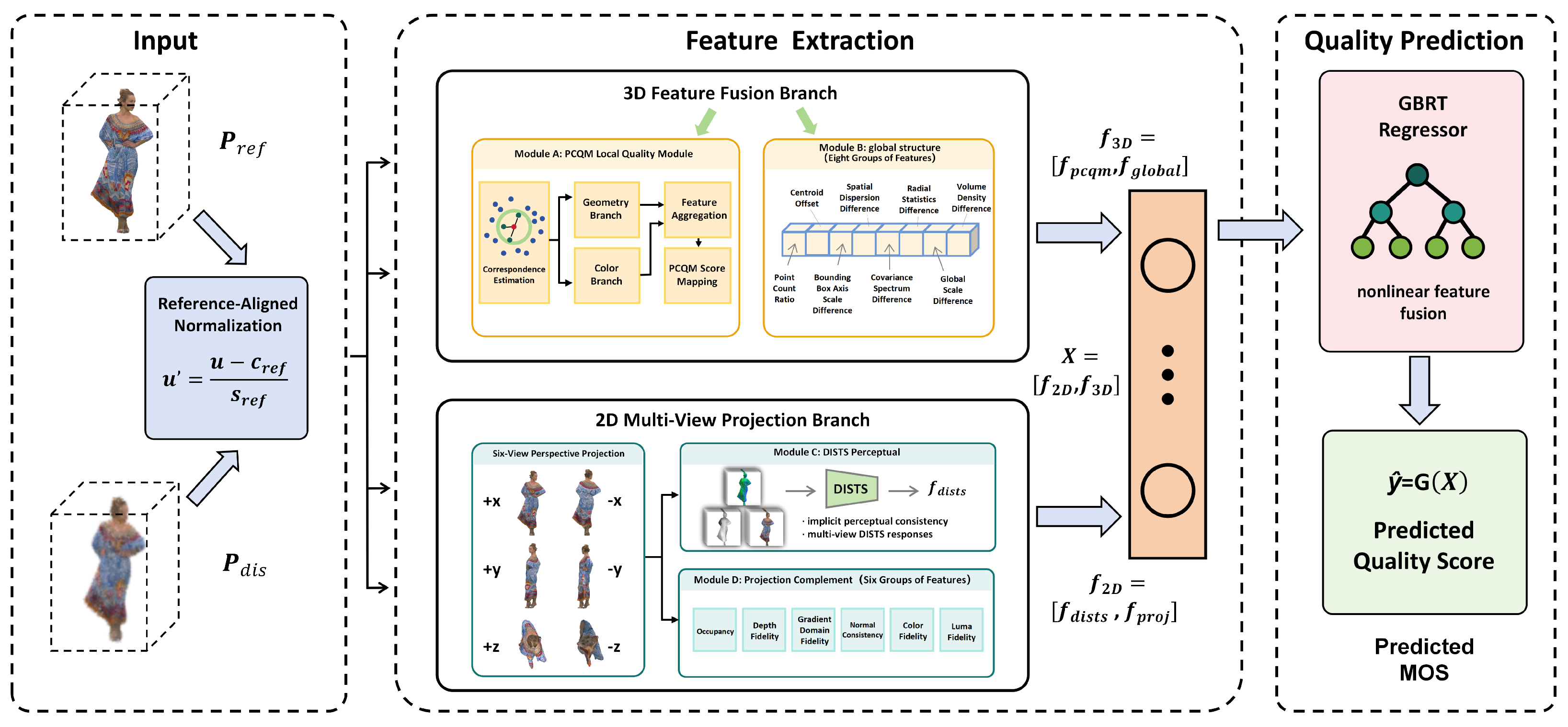
The proposed model is developed from the observation that strong baseline metrics are informative but incomplete. Following a feature fusion perspective guided by complementary perceptual and structural cues, we construct a dual branch model that combines multi-view projection features with 3D features. The overall architecture is shown in Figure 1.

3.1. Model Overview

The proposed model includes a 2D Multi-View Projection branch and a 3D Feature Fusion branch. In the 2D Multi-View Projection branch, DISTS [31] encodes perceptual similarity on projected views, while the proposed six feature subspaces describe occupancy mismatch and color and luma distortions. In the 3D Feature Fusion branch, PCQM [20] captures local geometry and color distortion, while the proposed global structural statistics characterize point count ratio, scale variation, and spatial dispersion differences. Let the reference and distorted point clouds be denoted by $P_{\mathrm{ref}}$ and $P_{\mathrm{dis}}$, respectively, and let the corresponding mean opinion score be y. The overall representation is defined as

$$\mathbf{x}=\left[{\mathbf{f}}_{2\mathrm{D}},{\mathbf{f}}_{3\mathrm{D}}\right],{\mathbf{f}}_{2\mathrm{D}}=\left[{\mathbf{f}}_{\mathrm{dists}},{\mathbf{f}}_{\mathrm{proj}}\right],{\mathbf{f}}_{3\mathrm{D}}=\left[{\mathbf{f}}_{\mathrm{pcqm}},{\mathbf{f}}_{\mathrm{global}}\right],\mathbf{y}=\mathcal{G}\left(\mathbf{x}\right).$$

(1)

Here, ${\mathbf{f}}_{\mathrm{dists}}$ denotes pretrained perceptual similarity features in the 2D projection domain, ${\mathbf{f}}_{\mathrm{proj}}$ denotes the six feature groups, ${\mathbf{f}}_{\mathrm{pcqm}}$ denotes local quality measurements in the 3D point domain, ${\mathbf{f}}_{\mathrm{global}}$ denotes global structural statistics, and $\mathcal{G}(·)$ is a regression function that maps the combined feature vector $\mathbf{x}$ to the predicted quality score y.

Specifically, ${\mathbf{f}}_{\mathrm{dists}}\in {\mathbb{R}}^{30}$ concatenates the six view responses and four summary statistics for each of the depth, normal, and color modalities, whereas ${\mathbf{f}}_{\mathrm{pcqm}}\in {\mathbb{R}}^{20}$ concatenates the nine raw PCQM outputs with nine validity indicators, the valid ratio, and the mapped PCQM score.

The two branch organization follows the different information represented in the 2D and 3D domains. Multi-view projections provide perceptual and appearance information under controlled viewing conditions, but they cannot fully preserve native 3D spatial properties. The 3D domain retains geometry and spatial distribution, while its local measurements do not directly provide the perceptual representation available from projected views. Within the 2D Multi-View Projection branch, DISTS measures perceptual similarity, whereas Projection explicitly quantifies Occupancy, Depth Fidelity, Gradient Domain Fidelity, Normal Consistency, Color Fidelity, and Luma Fidelity. Within the 3D Feature Fusion branch, PCQM measures local geometry and color quality, whereas Global structure explicitly describes point count, position, scale, spatial distribution, covariance, radial statistics, and density differences. Therefore, the motivation for designing the two branches is to extract features from different dimensions of the point cloud as comprehensively as possible, thereby improving the accuracy of the model’s quality prediction.

3.2. 2D Multi-View Projection Branch

The distorted point clouds are first normalized with respect to the reference point cloud. Let ${\mathbf{c}}_{\mathrm{ref}}$ be the centroid of the reference point cloud and $s_{\mathrm{ref}}$ be the maximum side length of its axis aligned bounding box. For any point $\mathbf{u}\in {\mathbb{R}}^3$, the aligned form under the reference frame is defined as

$${\mathbf{u}}^{\prime }={\displaystyle \frac{\mathbf{u}-{\mathbf{c}}_{\mathrm{ref}}}{s_{\mathrm{ref}}}}.$$

(2)

Under this reference frame, six canonical viewing directions are used to construct 2D perceptual views:

$$\mathcal{V}=\left\{+x,-x,+y,-y,+z,-z\right\},I_k^{\left(v\right)}=\mathcal{R}\left(P_k^{\prime };v\right),k\in \{\mathrm{ref},\mathrm{dis}\},v\in \mathcal{V}.$$

(3)

The positive and negative directions of the three orthogonal coordinate axes provide opposite observations along each spatial dimension. The fixed six view protocol also limits rendering and feature extraction cost while maintaining the same observation set for all contents.

Here, $P_k^{\prime }$ denotes the aligned version of point cloud $P_k$ under the reference frame, $I_k^{\left(v\right)}$ denotes the rendered image of point cloud $P_k$ observed from view v, $k\in \{\mathrm{ref},\mathrm{dis}\}$ indexes the reference and distorted point clouds, and $\mathcal{R}(·)$ denotes the rendering operator under fixed viewing parameters. The rendering resolution is $224\times 224$, and the six canonical directions are rendered using perspective projection with a field of view of ${60}^{\circ }$ and a single pixel point footprint. Open3D is used for point cloud loading and normal estimation, whereas a custom deterministic software rasterizer implemented with NumPy projects each point to the nearest image pixel to generate the depth, normal, and color maps; the occupancy and gradient fields are then derived from the rendered depth map. A software depth buffer retains the point with the smallest camera depth when multiple points are assigned to the same pixel. For each reference and distorted pair, the reference bounding box center defines the common observation center, the camera distance is twice the reference bounding sphere radius, and the same camera is used for both point clouds. For each view, the rendered result is decomposed into depth, normal, color, occupancy, and gradient fields:

$${\mathsf{\Psi }}_k^{\left(v\right)}=\left\{D_k^{\left(v\right)},N_k^{\left(v\right)},C_k^{\left(v\right)},M_k^{\left(v\right)},G_k^{\left(v\right)}\right\},M_k^{\left(v\right)}=\mathbb{I}\left(D_k^{\left(v\right)}>0\right),G_k^{\left(v\right)}={∥\nabla D_k^{\left(v\right)}∥}_2.$$

(4)

Here, ${\mathsf{\Psi }}_k^{\left(v\right)}$ denotes the multi-modal observation set of point cloud $P_k$ under view v, where $D_k^{\left(v\right)}$, $N_k^{\left(v\right)}$, and $C_k^{\left(v\right)}$ denote the depth, normal, and color fields, respectively; $M_k^{\left(v\right)}$ denotes the occupancy mask; and $G_k^{\left(v\right)}$ denotes the gradient magnitude field of depth.

This unified observation protocol enables the perceptual prior and the explicit error statistics in the 2D branch to be extracted from the same comparison basis. It also provides a consistent scale reference for the 3D branch.

Reference-based normalization establishes a common position and scale. Residual displacements caused by geometric distortion remain in the rendered observations and contribute to the DISTS responses through its structure and texture representations. For the explicit Projection features, limited overlap is handled by the adaptive comparison domain in Equation (7).

The 2D branch combines perceptual responses derived from IQA with the proposed six feature subspaces. DISTS [31] supplies a perceptual similarity prior on multi-view point cloud projections across depth, normal, and color modalities. The six feature subspaces then describe occupancy mismatch, geometric deviation, and color differences.

Specifically, DISTS perceptual responses are computed view by view in the depth, normal, and color modalities:

$$t_m^{\left(v\right)}=1-\mathrm{DISTS}\left(I_{m,\mathrm{ref}}^{\left(v\right)},I_{m,\mathrm{dis}}^{\left(v\right)}\right),m\in \{\mathrm{depth},\mathrm{norm},\mathrm{color}\},v\in \mathcal{V}.$$

(5)

Here, $I_{m,\mathrm{ref}}^{\left(v\right)}$ and $I_{m,\mathrm{dis}}^{\left(v\right)}$ denote the rendered images in modality m for the reference and distorted point clouds, respectively, and $t_m^{\left(v\right)}$ denotes the DISTS-based perceptual similarity response under view v.

Based on these responses, the 2D perceptual backbone features are written as

$${\mathbf{f}}_{\mathrm{dists}}=\mathcal{B}\left({\left\{t_m^{\left(v\right)}\right\}}_{m\in \{\mathrm{depth},\mathrm{norm},\mathrm{color}\},v\in \mathcal{V}}\right).$$

(6)

Here, $\mathcal{B}(·)$ aggregates perceptual responses across views into summary statistics of the perceptual backbone.

For each modality, the six view responses are retained and are followed by their mean, population standard deviation, minimum, and maximum. Thus, the DISTS representation is

$${\mathbf{f}}_{\mathrm{dists}}=\underset{m\in \{\mathrm{depth},\mathrm{norm},\mathrm{color}\}}{\parallel }\left[t_m^{\left(1\right)},\dots ,t_m^{\left(6\right)},{\mu }_m,{\sigma }_m,t_m^{\min },t_m^{\max }\right]\in {\mathbb{R}}^{30},$$

where ‖ denotes vector concatenation, ${\mu }_m={\displaystyle \frac{1}{6}}{\sum }_{v=1}^6{t}_m^{\left(v\right)}$, and ${\sigma }_m=\sqrt{{\displaystyle \frac{1}{6}}{\sum }_{v=1}^6{(t_m^{\left(v\right)}-{\mu }_m)}^2}$. The depth map is normalized to $[0,1]$ using the joint minimum and maximum of the valid reference and distorted depths in each view, and is replicated over three channels before DISTS evaluation. The rendered normal and RGB maps are clipped to $[0,1]$. Before feature extraction, the three channels are standardized using means $(0.485,0.456,0.406)$ and standard deviations $(0.229,0.224,0.225)$. The pretrained DISTS parameters are fixed during feature extraction, and the response retained in the descriptor is the similarity $1-\mathrm{DISTS}$ in Equation (5).

Projection Feature Subspaces

The six feature groups in Projection within the 2D Multi-View Projection branch were engineered according to distinct distortion effects observable in reference aligned views. Point removal and resampling change the projected support and may produce holes or additional occupied regions, which motivates Occupancy. Coordinate perturbation and geometry quantization change the projected depth values. Depth Fidelity measures the magnitude of these geometric differences, whereas Gradient Domain Fidelity emphasizes changes in depth slopes, boundaries, and local variation. Normal Consistency describes changes in surface orientation that are not fully represented by scalar depth differences. Color Fidelity measures RGB attribute differences, and Luma Fidelity separately describes luminance changes. The six groups therefore cover spatial support, projected geometry, surface orientation, and appearance under the same rendering protocol.

To compensate for the incomplete explicit error description of DISTS, the proposed six feature groups are computed under the same observation protocol. Since sparse projections may contain too few valid pixels, an adaptive comparison domain is introduced:

$${\mathsf{\Gamma }}^{\left(v\right)}=\left\{\begin{array}{cc}{\mathsf{\Omega }}_{\cap }^{\left(v\right)},\hfill & |{\mathsf{\Omega }}_{\cap }^{\left(v\right)}| \ge 32,\hfill \\ {\mathsf{\Omega }}_{\cup }^{\left(v\right)},\hfill & |{\mathsf{\Omega }}_{\cap }^{\left(v\right)}| <32\mathrm{and}|{\mathsf{\Omega }}_{\cup }^{\left(v\right)}| \ge 16,\hfill \\ \mathcal{I},\hfill & \mathrm{otherwise},\hfill \end{array}\right.$$

(7)

where ${\mathsf{\Omega }}_{\cap }^{\left(v\right)}$ and ${\mathsf{\Omega }}_{\cup }^{\left(v\right)}$ denote the intersection and union of the occupied regions in the reference and distorted views, respectively, and $\mathcal{I}$ denotes the complete image domain. Based on ${\mathsf{\Gamma }}^{\left(v\right)}$, the explicit error module is written as

$${\mathbf{f}}_{\mathrm{proj}}^{\left(v\right)}=\mathsf{\Phi }\left({\mathsf{\Psi }}_{\mathrm{ref}}^{\left(v\right)},{\mathsf{\Psi }}_{\mathrm{dis}}^{\left(v\right)};{\mathsf{\Gamma }}^{\left(v\right)}\right),{\mathbf{f}}_{\mathrm{proj}}=\mathcal{A}\left({\left\{{\mathbf{f}}_{\mathrm{proj}}^{\left(v\right)}\right\}}_{v\in \mathcal{V}}\right).$$

(8)

Here, ${\mathsf{\Psi }}_{\mathrm{ref}}^{\left(v\right)}$ and ${\mathsf{\Psi }}_{\mathrm{dis}}^{\left(v\right)}$ denote the multi-modal observation sets of the reference and distorted point clouds under view v, respectively. ${\mathbf{f}}_{\mathrm{proj}}^{\left(v\right)}$ denotes the explicit projection feature vector extracted from view v over the adaptive comparison domain ${\mathsf{\Gamma }}^{\left(v\right)}$. $\mathsf{\Phi }(·)$ collects explicit indicators for occupancy mismatch, geometric deviation, and chromatic discrepancy, including occupancy overlap, depth fidelity, gradient disturbance, normal consistency, color fidelity, and luminance similarity, and $\mathcal{A}(·)$ aggregates these interpretable error cues across the six views.

Let $a_i$ and $b_i$, $i=1,\dots ,n$, denote corresponding scalar samples from the reference and distorted fields over ${\mathsf{\Gamma }}^{\left(v\right)}$. The common error indicators are defined as

$$\begin{array}{cc}\hfill \mathrm{MAE}& ={\displaystyle \frac{1}{n}}{\displaystyle \sum _{i=1}^n}|a_i-b_i|,\mathrm{RMSE}=\sqrt{{\displaystyle \frac{1}{n}}\sum _{i=1}^n{(a_i-b_i)}^2},\hfill \\ \hfill \mathrm{PSNR}& =20{\log }_{10}L-10{\log }_{10}\left(\mathrm{MSE}\right).\hfill \end{array}$$

where the normalized data range is $L=1$ and PSNR is set to 100 when the MSE is smaller than ${10}^{-12}$. Global SSIM is calculated from the means, population variances, and population covariance of the two vectors, with $C_1={\left(0.01L\right)}^2$ and $C_2={\left(0.03L\right)}^2$. The 16 indicators are organized into the same six feature groups used throughout this paper: Occupancy contains occupancy IoU and the mean absolute difference between the binary occupancy masks; Depth Fidelity contains depth MAE, RMSE, PSNR, and SSIM; Gradient Domain Fidelity contains MAE and RMSE between the gradient magnitude fields; Normal Consistency contains the mean cosine similarity and the root mean square component difference between valid encoded normal vectors; Color Fidelity contains RGB MAE, RMSE, PSNR, and SSIM; and Luma Fidelity contains luma MAE and SSIM. Luma is calculated as $Y=0.299R+0.587G+0.114B$. For each indicator z, the aggregation operator is

$$\mathcal{A}\left(z\right)=\left[{\mathrm{mean}}_v\left(z^{\left(v\right)}\right),{\mathrm{std}}_v\left(z^{\left(v\right)}\right),\underset{v}{\min }\left(z^{\left(v\right)}\right),\underset{v}{\max }\left(z^{\left(v\right)}\right)\right],$$

where finite values from the six views are used and ${\mathrm{std}}_v$ denotes the population standard deviation. The 16 indicators therefore produce $16\times 4=64$ dimensions.

The final 2D branch is then given by

$${\mathbf{f}}_{2\mathrm{D}}=\left[{\mathbf{f}}_{\mathrm{dists}},{\mathbf{f}}_{\mathrm{proj}}\right].$$

(9)

Equation (9) shows that the 2D branch combines perceptual similarity with explicit and traceable evidence of occupancy mismatch, geometric deviation, and chromatic discrepancy.

3.3. 3D Feature Fusion Branch

The 3D Feature Fusion branch combines local measurements obtained from PCQM with global structural statistics computed directly from point clouds. PCQM effectively characterizes local geometry and color distortion, but it is less sensitive to point count change, scale variation, spatial redistribution, and density variation. Therefore, a compact global descriptor is introduced to complement it.

Specifically, the 3D local quality backbone consists of the raw PCQM outputs and their derived reliability variables:

$$\begin{array}{cc}\hfill {\mathbf{q}}_{\mathrm{pcqm}}& =\left[F_1,F_2,\dots ,F_8,S_{\mathrm{pcqm}}\right],\hfill \\ \hfill {\mathit{\nu }}_{\mathrm{pcqm}}& =\left[{\nu }_1,{\nu }_2,\dots ,{\nu }_9\right],{\nu }_i=\mathbb{I}\left(\mathrm{isfinite}\left({\left({\mathbf{q}}_{\mathrm{pcqm}}\right)}_i\right)\right),i=1,\dots ,9,\hfill \\ \hfill {\rho }_{\mathrm{valid}}& ={\displaystyle \frac{1}{9}}{\displaystyle \sum _{i=1}^9}{\nu }_i,s_{\mathrm{pcqm}}=-{\log }_{10}\max (S_{\mathrm{pcqm}},{10}^{-12}),\hfill \\ \hfill {\mathbf{f}}_{\mathrm{pcqm}}& =\left[{\mathbf{q}}_{\mathrm{pcqm}},{\mathit{\nu }}_{\mathrm{pcqm}},{\rho }_{\mathrm{valid}},s_{\mathrm{pcqm}}\right]\in {\mathbb{R}}^{20}.\hfill \end{array}$$

(10)

Here, $F_1,\dots ,F_8$ are the local geometric and color components of PCQM, $S_{\mathrm{pcqm}}$ is the overall score, ${\mathit{\nu }}_{\mathrm{pcqm}}$ stores validity indicators for the nine raw PCQM outputs, and ${\rho }_{\mathrm{valid}}$ and $s_{\mathrm{pcqm}}$ denote the valid ratio indicator and the score compression mapping, respectively.

The nine raw values are read directly from the PCQM output file generated with a radius factor of 0.004, 20 nearest neighbors, and $r_x=2.0$. Each finite output is assigned a validity indicator of one, while a nonfinite output is assigned zero. The nine indicators, the valid ratio ${\rho }_{\mathrm{valid}}$, and the score mapping $s_{\mathrm{pcqm}}$ form the 11 derived variables in Equation (10).

Global Structural Descriptors

The eight feature groups in Global structure were engineered to cover nonlocal changes that are not explicitly represented by the local measurements of PCQM. Point removal and resampling can change point count and spatial density, which motivates Point Count Ratio and Volume Density Difference. Centroid Offset describes global position change. Bounding Box Axis Scale Difference and Global Scale Difference describe axis specific and overall extent changes caused by scaling or geometric deformation. Spatial Dispersion Difference and Covariance Spectrum Difference describe coordinate spread and anisotropic spatial distribution, while Radial Statistics Difference describes changes in the distribution of distances from the centroid. The three covariance eigenvalue differences retain the principal variance information, so a separate anisotropy index is not introduced. Local curvature and neighborhood geometry are represented by PCQM, and surface orientation is represented by Normal Consistency in the 2D Multi-View Projection branch; these attributes are therefore not repeated as additional feature groups in Global structure.

To compensate for the incomplete global modeling ability of local measurements, the number of points, centroid, bounding box axis scale, global scale, spatial dispersion, covariance spectrum, radial statistics, and volumetric density are extracted directly from the raw point clouds. The global statistics set is defined as

$$S\left(P\right)=\left\{N,\mathbf{c},\mathbf{e},\delta ,\mathit{\sigma },\mathit{\lambda },\mathbf{r},\eta \right\}.$$

(11)

Here, $S\left(P\right)$ denotes the global statistics set of point cloud P, where N denotes the number of points, $\mathbf{c}$ denotes the centroid, $\mathbf{e}$ denotes the axis-aligned bounding-box extent vector, $\delta$ denotes the diagonal length of the bounding box, $\mathit{\sigma }$ denotes the coordinate-wise standard deviation vector of centered points, $\mathit{\lambda }$ denotes the covariance eigenvalue vector in descending order, $\mathbf{r}$ denotes the radial statistics term, and $\eta$ denotes the volumetric density. The statistics in Equation (11) summarize point count change, scale variation, spatial redistribution, and density variation at several geometric levels. Specifically, N and $\eta$ describe point count change and volumetric density, $\mathbf{e}$ and $\delta$ characterize axis wise and global scale variation, $\mathbf{c}$, $\mathit{\sigma }$, and $\mathit{\lambda }$ capture spatial redistribution and covariance spectrum change, and $\mathbf{r}$ captures radial distribution change.

Using the statistics of the reference point cloud as the anchor, the relative global structure offset vector of the distorted point cloud is written as

$${\mathbf{f}}_{\mathrm{global}}=\left[\begin{array}{c}{f}_N\\ f_c\\ {\mathbf{f}}_e\\ {\mathbf{f}}_{\sigma }\\ {\mathbf{f}}_{\lambda }\\ {\mathbf{f}}_r\\ f_{\delta }\\ f_{\eta }\end{array}\right]$$

(12)

$$f_N=\log \left({\displaystyle \frac{N_{\mathrm{dis}}+1}{N_{\mathrm{ref}}+1}}\right),f_c={\displaystyle \frac{{∥{\mathbf{c}}_{\mathrm{dis}}-{\mathbf{c}}_{\mathrm{ref}}∥}_2}{{\delta }_{\mathrm{ref}}}},$$

$${\mathbf{f}}_e={\displaystyle \frac{{\mathbf{e}}_{\mathrm{dis}}-{\mathbf{e}}_{\mathrm{ref}}}{\max ({\mathbf{e}}_{\mathrm{ref}},{ϵ}_g)}},$$

$${\mathbf{f}}_{\sigma }={\displaystyle \frac{{\mathit{\sigma }}_{\mathrm{dis}}-{\mathit{\sigma }}_{\mathrm{ref}}}{\max ({\mathit{\sigma }}_{\mathrm{ref}},{ϵ}_g)}},{\mathbf{f}}_{\lambda }={\displaystyle \frac{{\mathit{\lambda }}_{\mathrm{dis}}-{\mathit{\lambda }}_{\mathrm{ref}}}{\max ({\mathit{\lambda }}_{\mathrm{ref}},{ϵ}_g)}},$$

$${\mathbf{f}}_r={\displaystyle \frac{{\mathbf{r}}_{\mathrm{dis}}-{\mathbf{r}}_{\mathrm{ref}}}{\max ({\mathbf{r}}_{\mathrm{ref}},{ϵ}_g)}},$$

$$f_{\delta }={\displaystyle \frac{{\delta }_{\mathrm{dis}}-{\delta }_{\mathrm{ref}}}{{\delta }_{\mathrm{ref}}}},f_{\eta }={\displaystyle \frac{{\eta }_{\mathrm{dis}}-{\eta }_{\mathrm{ref}}}{\max ({\eta }_{\mathrm{ref}},{ϵ}_{\eta })}}.$$

Here, ${\mathbf{r}}_{\mathrm{ref}}$ and ${\mathbf{r}}_{\mathrm{dis}}$ denote the radial statistics vectors of the reference and distorted point clouds, respectively, and ${\mathbf{f}}_r$ denotes their relative offset.

In implementation, we set ${ϵ}_g={10}^{-3}$ and ${ϵ}_{\eta }={10}^{-6}$. For vector quantities, both $\max (·,{ϵ}_g)$ and the division are applied element wise.

For completeness, the centroid is the arithmetic mean of the point coordinates, the axis aligned bounding box extent is the coordinate wise maximum minus the coordinate wise minimum, and the global scale is the Euclidean norm of this extent vector. Spatial dispersion is the population standard deviation of the centered coordinates along the three axes. The covariance spectrum contains the three eigenvalues of the sample covariance matrix in descending order, with negative values caused by numerical error set to zero. Radial distance is the Euclidean distance from a point to the centroid, and the two radial statistics are its mean and population standard deviation. The bounding box volume is the product of the three axis extents after applying a lower bound of ${10}^{-12}$, and volume density is the number of points divided by this volume. The reference denominators of the Bounding Box Axis Scale Difference, Spatial Dispersion Difference, Covariance Spectrum Difference, and Radial Statistics Difference are lower bounded by ${10}^{-3}$. The denominator of Volume Density Difference is lower bounded by ${10}^{-6}$. These definitions give one Point Count Ratio, one Centroid Offset, three Bounding Box Axis Scale Difference components, three Spatial Dispersion Difference components, three Covariance Spectrum Difference components, two Radial Statistics Difference components, one Global Scale Difference, and one Volume Density Difference, for a total of 15 dimensions.

Equation (12) defines an explicit global structure compensation mechanism. The point count and density terms reflect sparsification or oversampling effects; the bounding box and global scale terms reflect scale variation; and the centroid, spatial dispersion, covariance spectrum, and radial statistics groups describe spatial redistribution caused by compression, resampling, or geometric perturbation. The final 3D branch is written as

$${\mathbf{f}}_{3\mathrm{D}}=\left[{\mathbf{f}}_{\mathrm{pcqm}},{\mathbf{f}}_{\mathrm{global}}\right].$$

(13)

Equation (13) shows that the 3D branch combines local geometry and color distortion cues from PCQM with global features describing point count changes, scale variation, spatial redistribution, and density variation.

3.4. Quality Regression and Fusion

After two branch level feature extractions are completed, the 2D and 3D descriptors are concatenated to form the unified representation $\mathbf{x}$. Then, a GBRT regressor is adopted to fuse the heterogeneous features. The final quality mapping is written as

$$\widehat{y}=c_0+{\displaystyle \sum _{m=1}^M}{\alpha }_m{h}_m\left(\tilde{\mathbf{x}}\right).$$

(14)

Here, $\widehat{y}$ denotes the predicted quality score, $\tilde{\mathbf{x}}$ denotes the fused feature vector after missing-value completion, $c_0$ denotes the initial bias term of the GBRT regressor, $h_m(·)$ denotes the regression tree at boosting stage m, ${\alpha }_m$ denotes the corresponding stage weight, and M denotes the total number of boosting stages.

Missing values are completed independently within each outer fold. For each feature dimension, a nonfinite value is replaced by the mean of the finite observations in the corresponding outer training fold, and the resulting mean is also used for the test fold. If no finite training observation is available, the completion value is set to zero. The completed 129 dimensional vector is provided directly to GBRT without feature standardization. The same configuration is used for all three datasets: squared error loss, 400 regression trees, a learning rate of 0.05, a subsample ratio of 0.7, a maximum tree depth of 2, a minimum of 3 samples per leaf, and a random seed of 2026.

The six feature groups in Projection and eight feature groups in Global structure were constructed according to distortion coverage and complementarity with DISTS and PCQM, rather than through dataset specific statistical screening of a candidate feature pool. Their composition is fixed for all three datasets, and the complete 129 dimensional descriptor is provided to GBRT for nonlinear regression. Module ablation, fine grained feature group analysis, and module level complementarity analysis evaluate the fixed feature composition, while the regressor comparison evaluates the choice of GBRT.

4. Experimental Results and Analysis

4.1. Experimental Setup

The proposed model is evaluated on three public FR-PCQA datasets: SJTU-PCQA, WPC, and ICIP2020. Since point cloud samples are strongly content dependent, all experiments use content level splits to avoid data leakage caused by placing the same content in both the training and test sets. Specifically, SJTU-PCQA uses a content level protocol with 9 folds, WPC uses a content level protocol with 10 folds, and ICIP2020 uses a protocol with 6 folds. The 2D projections are generated using the fixed software rasterization protocol described in Section 3.2. Performance is measured using four standard criteria: Spearman rank order correlation coefficient (SROCC), Pearson linear correlation coefficient (PLCC), Kendall rank order correlation coefficient (KRCC), and root mean square error (RMSE).

In implementation, the complete model contains two branches and four internal modules. The 2D branch consists of 30 dimensions of DISTS perceptual features and 64 dimensions of explicit projection error statistics, yielding 94 dimensions. The 3D branch consists of 20 dimensions of PCQM derived local quality features and 15 dimensions of global structural statistics, yielding 35 dimensions. Therefore, the fused representation has 129 dimensions. Specifically, the 64 projection dimensions are obtained by applying the same four summary operators to 16 view-wise indicators, including occupancy IoU and occupancy L1 mismatch, depth MAE/RMSE/PSNR/SSIM, gradient MAE/RMSE, normal cosine similarity and L2 error, color MAE/RMSE/PSNR/SSIM, and luma MAE/SSIM. The 15 global dimensions include point count ratio, centroid offset, three bounding-box axis scale differences, three spatial dispersion differences, three covariance-spectrum differences, radial mean difference, radial standard-deviation difference, global scale difference, and volume density difference. The fused representation is mapped to the final quality score using GBRT. Unless otherwise stated, all results in this section correspond to the full model.

Table 1. Composition of the 129 dimensional descriptor.

Branch	Component	Dim.	Composition
2D Multi-View Projection branch	DISTS	30	Three modalities, each containing six view responses and four summary statistics
	Projection	64	Occupancy (8), Depth Fidelity (16), Gradient Domain Fidelity (8), Normal Consistency (8), Color Fidelity (16), and Luma Fidelity (8)
3D Feature Fusion branch	PCQM	20	Nine raw outputs and 11 derived variables
	Global structure	15	Point Count Ratio (1), Centroid Offset (1), Bounding Box Axis Scale Difference (3), Spatial Dispersion Difference (3), Covariance Spectrum Difference (3), Radial Statistics Difference (2), Global Scale Difference (1), and Volume Density Difference (1)
Complete descriptor	Two branches	129	2D Multi-View Projection branch (94) and 3D Feature Fusion branch (35)

summarizes the descriptor composition and fixes the feature order used by GBRT.

The implementation uses Python 3.9 and scikit-learn 1.6.1. The feature ordering and GBRT configuration remain unchanged across SJTU-PCQA, WPC, and ICIP2020.

4.2. Overall Results

Table 2. Overall performance of the proposed model on the three datasets.

Dataset	SROCC	PLCC	KRCC	RMSE
SJTU-PCQA	0.91537	0.9227	0.7638	1.0576
WPC	0.9101	0.9122	0.7531	9.6413
ICIP2020	0.9778	0.9784	0.9166	0.2620

summarizes the overall performance on the three datasets. The proposed model achieves SROCC values of 0.91537, 0.9101, and 0.9778 on SJTU-PCQA, WPC, and ICIP2020, respectively. These results indicate strong ranking consistency across datasets with different content compositions and distortion distributions. The corresponding PLCC values further show that the fused representation supports a stable mapping to MOS values.

To compare the proposed model with representative FR-PCQA baselines,

Table 3. Performance comparison of different competing models on the three datasets.

Method	SJTU-PCQA			WPC			ICIP2020
	PLCC↑	SROCC↑	RMSE↓	PLCC↑	SROCC↑	RMSE↓	PLCC↑	SROCC↑	RMSE↓
PSNR	0.462	0.437	2.152	0.306	0.279	21.822	0.669	0.655	0.844
SSIM [32]	0.579	0.540	1.979	0.367	0.291	21.321	0.702	0.689	0.809
MS-SSIM [33]	0.621	0.566	1.902	0.384	0.316	21.168	0.720	0.789	0.695
GMSD [34]	0.635	0.570	1.876	0.343	0.298	21.536	0.724	0.698	0.784
FSIM [35]	0.575	0.521	1.985	0.304	0.232	21.839	0.741	0.709	0.763
VIF [36]	0.679	0.638	1.783	0.429	0.415	20.704	0.802	0.678	0.807
MSE-p2po [37]	0.877	0.791	1.166	0.578	0.566	18.708	0.888	0.878	0.522
Hausdorff-p2po [37]	0.742	0.681	1.628	0.398	0.258	21.028	0.601	0.542	0.908
MSE-p2pl [37]	0.753	0.676	1.596	0.488	0.446	20.013	0.913	0.915	0.463
Hausdorff-p2pl [37]	0.737	0.670	1.639	0.383	0.315	21.171	0.649	0.602	0.865
PSNRYUV [37]	0.652	0.646	1.841	0.551	0.536	19.132	0.868	0.564	0.867
PCQM [20]	0.860	0.847	1.237	0.751	0.743	15.132	0.969	0.970	0.280
GraphSIM [21]	0.856	0.841	1.071	0.694	0.680	16.498	0.890	0.872	0.518
MS-GraphSIM [38]	0.897	0.874	1.071	0.717	0.707	15.970	0.906	0.895	0.481
pointSSIM [22]	0.725	0.704	1.672	0.510	0.454	19.713	0.904	0.865	0.486
PHM [5]	0.921	0.901	1.066	0.842	0.836	12.499	0.971	0.966	0.279
FRSVR [7]	0.872	0.855	1.239	0.834	0.822	13.292	0.966	0.973	0.367
PW-SCQA [4]	0.875	0.899	1.518	0.829	0.835	14.367	0.839	0.959	0.698
Ours	0.923	0.915	1.058	0.912	0.910	9.641	0.978	0.978	0.262

reports the results of a broad set of competing methods on the three datasets. The baselines include projection domain metrics such as PSNR, SSIM, MS-SSIM, and VIF, point domain or hybrid metrics such as MSE-p2po, MSE-p2pl, PCQM, GraphSIM, and MS-GraphSIM, and learning based or perception guided baselines such as FRSVR, PHM, and PW-SCQA.

All competing methods in Table 3 were reproduced using the same content-level splits as the proposed model. For methods whose raw quality scores are not expressed on the MOS scale, a four-parameter logistic function was fitted using only the training contents within each outer fold and then applied to the corresponding test contents before PLCC and RMSE were computed. For these methods, SROCC was calculated directly from the raw scores.

Table 3 shows that the proposed model achieves the highest PLCC and SROCC values and the lowest RMSE on the three evaluated datasets. Compared with representative point domain metrics such as PCQM, GraphSIM, and MS-GraphSIM, the gains are particularly clear on WPC and SJTU-PCQA. The proposed model also performs favorably compared with the learning based baseline FRSVR. These results suggest that the proposed FR-PCQA method can provide a more complete description of the distortions.

The best performance is achieved on the ICIP2020 dataset, where distortions are dominated by compression and are relatively concentrated. SJTU-PCQA and WPC are more challenging because they contain broader distortion diversity and larger perceptual variability. Overall, the proposed dual branch model maintains stable performance across all three datasets, indicating robustness under heterogeneous distortion conditions.

To examine generalization under changes in data distribution, we conduct six directed database transfer experiments among SJTU-PCQA, WPC, and ICIP2020. For each experiment, the model is trained on one database and directly evaluated on another. Missing values are completed using statistics estimated from the training database, and no score mapping is estimated from the test database. SROCC, PLCC, and KRCC are reported because the databases use different MOS scales.

As shown in

Table 4. Cross database performance of the proposed model.

Training Database	Test Database	SROCC	PLCC	KRCC
SJTU-PCQA	WPC	0.7091	0.6803	0.5127
SJTU-PCQA	ICIP2020	0.8982	0.8979	0.7248
WPC	SJTU-PCQA	0.8195	0.8355	0.6237
WPC	ICIP2020	0.8740	0.8541	0.7003
ICIP2020	SJTU-PCQA	0.7969	0.7861	0.6099
ICIP2020	WPC	0.5816	0.5008	0.4581

, transfer performance varies with the training and test databases. Training on SJTU-PCQA and WPC yields SROCC values of 0.8982 and 0.8740 on ICIP2020, respectively, while training on WPC and testing on SJTU-PCQA yields an SROCC of 0.8195. The lowest SROCC of 0.5816 is obtained when the model is trained on ICIP2020 and tested on WPC. These results demonstrate the ability of the proposed model to transfer across databases, while also showing that its performance is influenced by differences between the training and test data distributions.

Robustness under controlled external perturbations is further examined using 18 samples from SJTU-PCQA, with two samples selected from approximately the lower and upper MOS tertiles of each source content. Each sample is evaluated using a model trained without its source content. Joint rotations of 15 and 30 degrees about the $[1,1,1]$ axis are applied to both the reference and distorted point clouds to examine pose stability. Geometry noise with standard deviations of 0.05% and 0.10% of the reference bounding box diagonal and random point removal ratios of 5% and 10% are applied to the distorted point cloud. A fixed random seed of 2026 is used.

Table 5. Prediction responses under controlled external perturbations on SJTU-PCQA. $\Delta$ denotes the perturbed prediction minus the original prediction.

Perturbation	Level	SROCC	Mean $\Delta$	Mean $|\Delta |$	Decrease (%)
Joint rotation	${15}^{\circ }$	0.9133	0.2622	0.3787	–
Joint rotation	${30}^{\circ }$	0.8080	0.3706	0.4562	–
Geometry noise	0.05%	0.8514	$-0.4503$	0.4749	77.8
Geometry noise	0.10%	0.8328	$-1.5303$	1.5303	100.0
Point removal	5%	0.9897	0.0122	0.2043	50.0
Point removal	10%	0.9794	0.0020	0.2114	33.3

shows that joint rotation largely preserves the prediction ranking at 15 degrees, while the lower SROCC at 30 degrees indicates increased sensitivity to larger changes in orientation. Geometry noise produces a clear decrease in the predicted quality, and the stronger noise level results in a lower prediction than the weaker level for all 18 samples. Random point removal maintains high rank correlations, but its effect on the absolute predictions is not consistently directional. These results indicate that the response of the proposed model depends on both the type and intensity of the external perturbation.

4.3. Statistical Significance Analysis

To examine whether the performance differences are consistent across content splits, we conduct paired comparisons with PHM, FRSVR, and PW-SCQA using results obtained from the same outer test folds. For each fold, we define $\Delta \mathrm{SROCC}={\mathrm{SROCC}}_{\mathrm{Ours}}-{\mathrm{SROCC}}_{\mathrm{Baseline}}$. The 95% confidence intervals are estimated using 20,000 iterations of a paired percentile bootstrap over the outer folds. A two-sided exact permutation test based on sign changes is applied to the fold differences, and the resulting p values are adjusted within each dataset using the Holm procedure.

Table 6. Paired significance comparisons with recent baselines. Positive $\Delta$SROCC favors the proposed model. Bold values indicate statistical significance at the 0.05 level after Holm correction.

Dataset	Baseline	$\Delta$SROCC	95% CI	Holm Adjusted p
SJTU-PCQA	PHM	0.0136	[$-0.0174$, 0.0431]	0.418
	FRSVR	0.0589	[0.0120, 0.1242]	0.059
	PW-SCQA	0.0160	[$-0.0036$, 0.0364]	0.352
WPC	PHM	0.0738	[0.0344, 0.1093]	0.020
	FRSVR	0.0878	[0.0535, 0.1203]	0.012
	PW-SCQA	0.0746	[0.0392, 0.1074]	0.020
ICIP2020	PHM	0.0119	[0.0006, 0.0250]	0.750
	FRSVR	0.0039	[$-0.0039$, 0.0134]	0.750
	PW-SCQA	0.0191	[$-0.0042$, 0.0453]	0.750

reports the results.

On WPC, the mean SROCC improvements over PHM, FRSVR, and PW-SCQA are 0.0738, 0.0878, and 0.0746, respectively, and all three differences remain significant after Holm correction. On SJTU-PCQA and ICIP2020, the proposed model achieves positive mean differences in all comparisons, while the adjusted p values are above 0.05. These results provide statistical evidence for the performance gains on WPC and show higher mean SROCC under the evaluated folds on SJTU-PCQA and ICIP2020.

4.4. Regressor Comparison

To evaluate the performance of the GBRT, we compare it with other classic regressors, as an example, support vector regression (SVR), Random Forest, AdaBoost, and a multilayer perceptron (MLP) with three hidden layers. SVR, Random Forest, AdaBoost, and MLP were selected to represent kernel regression, bagging ensembles, boosting ensembles, and neural network regression, respectively. All regressors use the same feature representation with 129 dimensions and the same protocols with content independent outer folds. GBRT uses the fixed configuration of the full model, while the parameters of the comparison regressors are selected by content level cross validation with three folds within each outer training fold. Random Forest, AdaBoost, and MLP are evaluated with three random seeds, and their results are first averaged within each outer test fold.

Table 7. Performance comparison of different regressors using the same 129 dimensional feature representation.

Dataset	Regressor	SROCC (Mean ± SD)	PLCC	KRCC	RMSE
SJTU-PCQA	GBRT	$0.91537\pm 0.0334$	0.9227	0.7638	1.0576
	SVR	$0.8632\pm 0.1100$	0.8625	0.7033	1.2943
	Random Forest	$0.9085\pm 0.0434$	0.9168	0.7571	1.0622
	AdaBoost	$0.9010\pm 0.0419$	0.9106	0.7475	1.0956
	MLP	$0.8368\pm 0.1530$	0.8101	0.6848	1.9314
WPC	GBRT	$0.9101\pm 0.0358$	0.9122	0.7531	9.6413
	SVR	$0.8772\pm 0.1020$	0.8859	0.7151	10.8086
	Random Forest	$0.9181\pm 0.0249$	0.9216	0.7642	9.2816
	AdaBoost	$0.9064\pm 0.0249$	0.9024	0.7444	10.3436
	MLP	$0.8786\pm 0.0453$	0.8783	0.7096	12.1434
ICIP2020	GBRT	$0.9778\pm 0.0209$	0.9784	0.9166	0.2620
	SVR	$0.9421\pm 0.0635$	0.9558	0.8529	0.3373
	Random Forest	$0.9752\pm 0.0228$	0.9765	0.9155	0.2601
	AdaBoost	$0.9747\pm 0.0209$	0.9751	0.9110	0.2548
	MLP	$0.9507\pm 0.0227$	0.9204	0.8456	0.5765

reports the mean results across the outer folds, together with the standard deviation of SROCC.

As shown in Table 7, GBRT achieves the highest SROCC, PLCC, and KRCC values on SJTU-PCQA and ICIP2020 datasets, while Random Forest achieves the highest correlation values on WPC. AdaBoost obtains the lowest RMSE on ICIP2020. GBRT consistently outperforms SVR and MLP on all four criteria across the three datasets. The measured prediction times of GBRT are 0.026, 0.018, and 0.067 ms per sample on SJTU-PCQA, WPC, and ICIP2020, respectively, whereas Random Forest requires 2.344, 1.275, and 5.769 ms per sample. These results show that GBRT can provide consistently high correlation values across the three datasets with a low prediction cost.

4.5. Computational Complexity

This section examines computational complexity through measured running time.

Table 8. Comparison of feature extraction time and total running time. Values are reported as mean runtime in seconds over 20 point cloud pairs.

Dataset	Method	Feature Extraction	Total Runtime
SJTU-PCQA	FRSVR	$14.269$	$14.269$
	PHM	$34.401$	$34.401$
	Ours	$54.152$	$54.153$
WPC	FRSVR	$22.439$	$22.439$
	PHM	$63.150$	$63.150$
	Ours	$39.795$	$39.796$
ICIP2020	FRSVR	$8.121$	$8.121$
	PHM	$30.187$	$30.187$
	Ours	$26.109$	$26.109$

reports the feature extraction time and total running time of FRSVR, PHM, and the proposed model on 20 point cloud pairs from each database. Experiments are performed on a workstation equipped with an Intel Core i7-14650HX CPU, 16 GB of memory, and an NVIDIA GeForce RTX 4060 Laptop GPU.

As shown in Table 8, FRSVR has the shortest running time on the three databases. The proposed model is faster than PHM on WPC and ICIP2020 but slower on SJTU-PCQA. Feature extraction accounts for nearly all of its total running time, with the main computational cost arising from PCQM and the rendering of six views. With the fixed settings used in this work, the average time complexity of the proposed model with respect to the point count is $O\left(N\log N\right)$.

4.6. Ablation Study

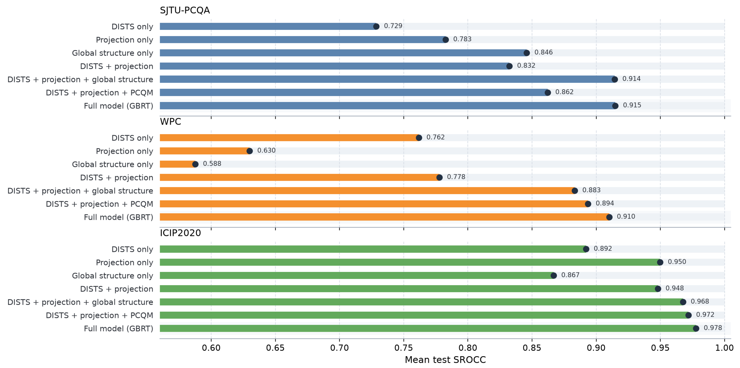
To quantify the contribution of each internal module and the final fusion strategy, seven ablation settings are evaluated: DISTS only, projection only, global structure only, DISTS + projection, DISTS + projection + global structure, DISTS + projection + PCQM, and full model (GBRT). Although the architecture contains two main branches, the ablations are conducted at the module level to identify the source of the complementary gain. A dedicated pairwise comparison is also reported to isolate the internal complementarity of the 2D and 3D branches. The overall ablation trend is shown in Figure 2.

Table 9. Pairwise complementary validation of the 2D and 3D branches. Best results within each triplet of branch configurations are shown in bold.

Branch	Configuration	SJTU-PCQA		WPC		ICIP2020
		SROCC↑	PLCC↑	SROCC↑	PLCC↑	SROCC↑	PLCC↑
2D branch	DISTS only	0.7286	0.7761	0.7617	0.7643	0.8921	0.8894
	Projection only	0.7826	0.8294	0.6299	0.6414	0.9498	0.9458
	DISTS + projection	0.8324	0.8466	0.7777	0.7778	0.9480	0.9364
3D branch	PCQM only	0.8595	0.9013	0.8924	0.8998	0.9701	0.9721
	Global structure only	0.8459	0.8805	0.5875	0.6240	0.8668	0.8540
	PCQM + global structure	0.8991	0.9182	0.9057	0.9094	0.9748	0.9755

directly evaluates the two branch level complementary hypotheses. In the 2D branch, DISTS + projection consistently outperforms DISTS only on all three datasets and exceeds projection only on SJTU-PCQA and WPC. On ICIP2020, projection only gives the highest SROCC and PLCC within the 2D branch, whereas DISTS + projection gives a higher KRCC, increasing it from 0.8467 to 0.8562, and reduces RMSE from 0.4899 to 0.4637. This pattern indicates that combining perceptual similarity with occupancy mismatch, geometric deviation, and chromatic discrepancy provides more balanced performance across the evaluation criteria.

In the 3D branch, the complementarity is stronger and more consistent. PCQM + global structure outperforms both PCQM only and global structure only on SJTU-PCQA, WPC, and ICIP2020. Compared with PCQM only, the SROCC gains are +0.0396, +0.0133, and +0.0048 on the three datasets, respectively, and PLCC also improves in all cases. This observation is consistent with the role of the global descriptor.

On SJTU-PCQA, the SROCC values of DISTS only, projection only, and global structure only are 0.7286, 0.7826, and 0.8459, respectively. These values indicate that global structural statistics alone are more informative than either 2D component on this dataset. When DISTS and projection features are combined, SROCC increases to 0.8324. Adding the 3D global structure module further increases SROCC to 0.9144, which is already close to the full model result. This behavior is consistent with the distortion composition of SJTU-PCQA, where downscaling and geometry noise strongly affect point count change, scale variation, spatial redistribution, and density variation. Accordingly, bounding box scale, global scale, radial distribution, volumetric density, and covariance spectrum descriptors provide important evidence that is not sufficiently captured by local PCQM responses. Adding PCQM only increases SROCC from 0.9144 to 0.91537, indicating that the dominant gain on this dataset comes from global structural compensation, while local geometry and color distortion cues mainly refine PLCC and RMSE.

On WPC, the SROCC values of DISTS only, projection only, and global structure only are 0.7617, 0.6299, and 0.5875, respectively. These values indicate that no single module can adequately describe the complex distortions in this dataset. Starting from the 2D combination DISTS + projection, adding either the global structure module or the PCQM module increases SROCC to 0.8832 and 0.8937, respectively, while the full model further reaches 0.9101. This pattern suggests that WPC contains both point count change, scale variation, spatial redistribution, and density variation described by global structural statistics, as well as local geometry and color distortion described by PCQM evidence. Thus, both components of the 3D branch are necessary.

On ICIP2020, the projection only configuration already reaches an SROCC of 0.9498, which is higher than the values of DISTS only (0.8921) and global structure only (0.8668). This indicates that occupancy mismatch, geometric deviation, and chromatic discrepancy in the 2D projection domain are highly sensitive to compression distortion. The full model further improves SROCC to 0.9778, showing that local geometry and color distortion, point count change, scale variation, spatial redistribution, and density variation still provide stable gains even when the 2D explicit error module is strong.

In addition to the module-based ablation experiments, we further evaluate the performance of the six groups of features in the proposed 2D branch and the eight groups of features in the 3D branch. In the experiment, the SJTU-PCQA dataset is employed since it contains geometry, color, downsampling, octree compression, and mixed distortions. To evaluate the contribution of a specific feature group, we remove it from the full feature set while maintaining all other settings. The contribution is then measured as the difference between the SROCC value of the complete feature set and that of the set without the target group. Therefore, $\Delta \mathrm{SROCC}$ is defined as $\Delta \mathrm{SROCC}={\mathrm{SROCC}}_{\mathrm{Full}}-{\mathrm{SROCC}}_{\mathrm{without}}$, where a larger positive value indicates a greater contribution. The specific results for each feature group are shown in

Table 10. The $\Delta \mathrm{SROCC}$ value for each feature group on SJTU-PCQA dataset.

Module	Feature Group	$\Delta$SROCC
Projection	Occupancy	+0.0027
	Depth Fidelity	+0.0031
	Gradient Domain Fidelity	+0.0026
	Normal Consistency	+0.0035
	Color Fidelity	+0.0011
	Luma Fidelity	+0.0018
Global structure	Point Count Ratio	+0.0185
	Centroid Offset	+0.0017
	Bounding Box Axis Scale Difference	+0.0013
	Spatial Dispersion Difference	+0.0057
	Covariance Spectrum Difference	+0.0044
	Radial Statistics Difference	+0.0021
	Global Scale Difference	+0.0013
	Volume Density Difference	+0.0012

.

As shown in Table 10, all the $\Delta \mathrm{SROCC}$ values are positive, indicating that all the proposed feature groups contribute positively to the final quality prediction. The maximum and minimum values are 0.0185 and 0.0011, respectively. Specially, for the projection module, the $\Delta \mathrm{SROCC}$ values for Occupancy, Depth Fidelity, Gradient Domain Fidelity, Normal Consistency, Color Fidelity, and Luma Fidelity are 0.0027, 0.0031, 0.0026, 0.0035, 0.0011, and 0.0018, respectively. For global structure module, the $\Delta \mathrm{SROCC}$ values for Point Count Ratio, Centroid Offset, Bounding Box Axis Scale Difference, Spatial Dispersion Difference, Covariance Spectrum Difference, Radial Statistics Difference, Global Scale Difference, and Volume Density Difference are 0.0185, 0.0017, 0.0013, 0.0057, 0.0044, 0.0021, 0.0013, and 0.0012, respectively.

4.7. Distortion Type Analysis

To further analyze the behavior of the model under different degradation scenarios, samples are grouped by both distortion category and specific distortion type.

Table 11. SROCC results under different distortion categories on the three datasets. A dash indicates that the corresponding category is not present in the dataset.

Distortion Category	SJTU-PCQA	WPC	ICIP2020
Geometry	0.8949	0.8912	–
Color	0.7611	0.9096	–
Compression	0.7181	0.8954	0.9634
Mixed	0.9156	0.7832	–

reports SROCC values under geometry, color, compression, and mixed distortions, while

Table 12. SROCC results under different specific distortion types on the three datasets.

Dataset	Distortion Type	SROCC
SJTU-PCQA	Color Noise	0.7611
SJTU-PCQA	Downscaling	0.8747
SJTU-PCQA	Downscaling + Color Noise	0.9049
SJTU-PCQA	Downscaling + Geometry Gaussian Noise	0.9176
SJTU-PCQA	Octree Compression	0.7181
SJTU-PCQA	Color + Geometry Gaussian Noise	0.9143
SJTU-PCQA	Geometry Gaussian Noise	0.9175
WPC	Color Quantization	0.9021
WPC	Geometry/Color QP Compression	0.8136
WPC	Gaussian Geometry/Color Noise	0.7832
WPC	Geometry Quantization	0.8912
WPC	Octree Compression	0.8784
WPC	Color Noise	0.9025
ICIP2020	G-PCC Octree Compression	0.9550
ICIP2020	G-PCC Trisoup Compression	0.9536
ICIP2020	V-PCC Compression	0.9182

provides a finer grained breakdown by distortion type.

Table 11 shows that, on SJTU-PCQA, the model performs most stably on mixed and geometry distortions, with SROCC values of 0.9156 and 0.8949, respectively. In contrast, pure color distortion and compression distortion yield lower SROCC values of 0.7611 and 0.7181. This result suggests that the proposed model is sensitive to large scale geometric change and mixed structural degradation, while pure color degradation and certain compression cases remain more challenging.

The results on WPC are more balanced. The color, compression, and geometry categories yield SROCC values of 0.9096, 0.8954, and 0.8912, respectively, whereas the mixed category decreases to 0.7832. This indicates that coupled geometry and color noise produces a more complex perceptual pattern and reduces ranking accuracy. ICIP2020 contains only compression distortions, yet the model still achieves an overall SROCC of 0.9634 for this category. As shown in Table 12, the predictions are most stable for G-PCC Octree and G-PCC Trisoup compression, whereas V-PCC compression is slightly more challenging. This suggests that different compression mechanisms induce different perceptual degradation patterns.

4.8. Small Sample Robustness

To evaluate sensitivity to the amount of available training content, we conduct repeated content sampling under content independent outer fold protocols. SJTU-PCQA and ICIP2020 use one content out protocols with 9 and 6 outer folds, respectively, while WPC uses 10 content independent outer folds, each containing two test contents. For each outer fold, the test contents remain fixed, and the specified number of reference contents is sampled without replacement from the remaining training pool. All distorted point clouds derived from a selected reference content are retained together in the training set. The numbers of training contents are $\{2,4,6,8\}$ for SJTU-PCQA, $\{4,8,12,16,18\}$ for WPC, and $\{2,3,4,5\}$ for ICIP2020. For each reduced setting, the sampling procedure is repeated 20, 12, and 20 times per outer fold, respectively. The full setting is evaluated once because it contains the complete training pool of the corresponding outer fold. A base seed of 2026 is used, and the seed for repetition r in outer fold k with m training contents is $2026+1000m+97k+r$.

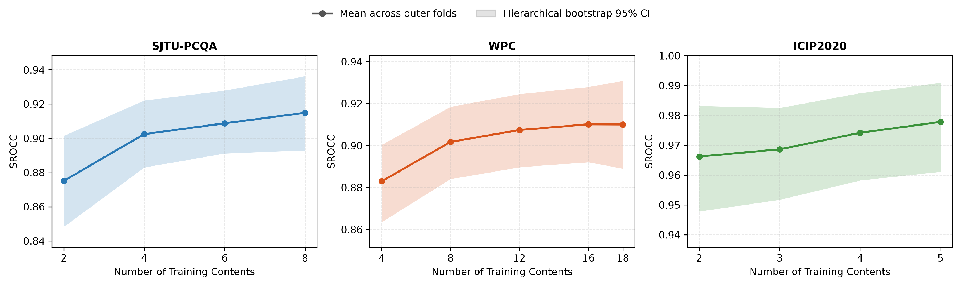
The SROCC values obtained from repeated training subsets are first averaged within each outer test fold. The resulting 9, 10, and 6 outer fold means are used to calculate the overall mean and sample standard deviation. The 95% confidence intervals (CIs) are estimated using 20,000 iterations of a hierarchical percentile bootstrap that resamples the outer folds and the repeated training subsets within each selected fold.

Table 13. Small sample robustness results. SD is calculated across outer fold means, and CIs are obtained by hierarchical bootstrap.

Dataset	Training Contents	SROCC (Mean ± SD)	95% CI
SJTU-PCQA	2	$0.8752\pm 0.0427$	$[0.8483,0.9015]$
	4	$0.9024\pm 0.0315$	$[0.8829,0.9221]$
	6	$0.9088\pm 0.0298$	$[0.8912,0.9279]$
	8 (full)	$0.91537\pm 0.0334$	$[0.8947,0.9356]$
WPC	4	$0.8830\pm 0.0304$	$[0.8635,0.9003]$
	8	$0.9018\pm 0.0290$	$[0.8841,0.9185]$
	12	$0.9074\pm 0.0294$	$[0.8897,0.9245]$
	16	$0.9102\pm 0.0308$	$[0.8921,0.9279]$
	18 (full)	$0.9101\pm 0.0358$	$[0.8890,0.9308]$
ICIP2020	2	$0.9662\pm 0.0245$	$[0.9478,0.9832]$
	3	$0.9686\pm 0.0213$	$[0.9517,0.9825]$
	4	$0.9742\pm 0.0203$	$[0.9582,0.9874]$
	5 (full)	$0.9778\pm 0.0209$	$[0.9612,0.9909]$

reports the mean, standard deviation, and confidence interval, and Figure 3 shows the corresponding means and 95% CIs.

For the paired comparisons, each fold mean obtained with a reduced setting is compared with the full setting evaluated on the same outer test fold. We report $\Delta \mathrm{SROCC}={\mathrm{SROCC}}_{\mathrm{full}}-{\mathrm{SROCC}}_{\mathrm{reduced}}$, its paired hierarchical bootstrap 95% CI, and the result of a two-sided exact permutation test based on sign changes in the fold level differences. The resulting p values are adjusted within each dataset using the Holm procedure, as reported in

Table 14. Paired comparisons between reduced and full settings on the same outer test folds. Positive $\Delta$SROCC favors the full setting. Bold values indicate statistical significance at the 0.05 level after Holm correction.

Dataset	Reduced vs. Full	$\Delta$SROCC	95% CI	Holm Adjusted p
SJTU-PCQA	2 vs. 8	0.0397	$[0.0231,0.0586]$	0.0117
	4 vs. 8	0.0124	$[0.0010,0.0228]$	0.1406
	6 vs. 8	0.0061	$[-0.0051,0.0152]$	0.2773
WPC	4 vs. 18	0.0271	$[0.0136,0.0385]$	0.0234
	8 vs. 18	0.0084	$[-0.0028,0.0168]$	0.3809
	12 vs. 18	0.0027	$[-0.0037,0.0082]$	0.7813
	16 vs. 18	$-0.0001$	$[-0.0063,0.0046]$	0.9863
ICIP2020	2 vs. 5	0.0116	$[0.0043,0.0206]$	0.1875
	3 vs. 5	0.0092	$[0.0043,0.0139]$	0.1875
	4 vs. 5	0.0036	$[-0.0002,0.0082]$	0.1875

.

The results show that the difference from the full setting generally decreases as the number of training contents increases. Compared with the corresponding full setting, the use of two training contents on SJTU-PCQA and four training contents on WPC decreases SROCC by 0.0397 and 0.0271, respectively. Both differences are statistically significant after Holm correction. The differences for six versus eight training contents on SJTU-PCQA and for 8, 12, or 16 versus 18 training contents on WPC are not statistically significant. For ICIP2020, the mean SROCC differences range from 0.0036 to 0.0116, and none of the paired comparisons is statistically significant after Holm correction. The standard deviations and confidence intervals quantify the variation across outer test folds under the evaluated training settings.

4.9. Module Level Complementarity Analysis

To examine the complementarity of the four internal feature blocks introduced in Section 3, the mean absolute correlation coefficients within and between the blocks are computed. Specifically, a Pearson correlation matrix is computed over the complete feature set, and block wise averages are then calculated for the DISTS module, the projection module, the global structure module, and the PCQM module.

Table 15. Within group and between group mean absolute correlation on different datasets.

Dataset	Within Group Correlation	Between Group Correlation	Difference
SJTU-PCQA	0.3975	0.2249	0.1726
WPC	0.4090	0.2122	0.1967
ICIP2020	0.5140	0.3167	0.1973
Overall	0.4402	0.2513	0.1889

reports the within group mean correlation, the between group mean correlation, and their difference for each dataset, while

Table 16. Aggregated block correlation matrix of the four internal feature modules (mean absolute correlation coefficient).

Module	Global Structure	Projection	DISTS	PCQM
global structure	0.3913	0.2179	0.2301	0.1290
projection	0.2179	0.4652	0.5080	0.1752
DISTS	0.2301	0.5080	0.7226	0.2475
PCQM	0.1290	0.1752	0.2475	0.1816

reports the aggregated block correlation matrix across all three datasets.

Table 15 shows that the within group mean absolute correlations are 0.3975, 0.4090, and 0.5140 on SJTU-PCQA, WPC, and ICIP2020, respectively. These values are higher than the corresponding between group mean absolute correlations of 0.2249, 0.2122, and 0.3167. After aggregation across the three datasets, the within group and between group correlations are 0.4402 and 0.2513, respectively, with a difference of 0.1889. These results indicate that the four internal modules form a stable block structure. They also support the intended complementarity between perceptual similarity and occupancy mismatch, geometric deviation, and chromatic discrepancy in the 2D branch, and between local geometry and color distortion and global structural statistics in the 3D branch.

Table 16 further shows that the global structure module has generally low correlations with the other modules, especially with the PCQM module, for which the mean correlation is only 0.1290. The PCQM module also has correlations below 0.25 with all other modules. This indicates that the “local geometry and color distortion + global structural statistics” design within the 3D branch provides two relatively independent types of evidence. In contrast, the mean correlation between projection and DISTS is 0.5080, which is higher than most cross group values. This is reasonable because both modules share the same projection observation protocol: the former describes occupancy mismatch, geometric deviation, and chromatic discrepancy, whereas the latter captures perceptual similarity. Combined with the ablation results, these findings indicate that the dual branch organization exhibits low redundancy and meaningful complementarity across its internal modules.

5. Conclusions

This paper presents a dual branch multi-view projection and 3D feature fusion model for full-reference point cloud quality assessment. The model is built on complementary evidence from the 2D projection domain and the native 3D point domain. The central idea is to combine perceptual similarity with the proposed six groups of features in the 2D projection domain, and to combine local geometry and color distortion with the proposed global structure features in the 3D point domain. The two branches are fused by GBRT to produce a compact and interpretable FR-PCQA model.

Experiments on SJTU-PCQA, WPC, and ICIP2020 show that the proposed model achieves stable and competitive results in benchmark comparison, ablation studies, evaluation by distortion type, and small sample analysis. Overall, the results support the main claim of this paper: fusing the above projection and 3D space features improves predictive performance while keeping the model interpretable on three public datasets. The present implementation has two practical limitations: it uses a fixed projection protocol with six views and depends on the availability of DISTS and PCQM descriptors, which may affect sensitivity to artifacts caused by viewpoint changes and efficiency in large scale deployment. While the six canonical directions provide a consistent basis, they may offer incomplete coverage for asymmetric content or localized distortions. The number and selection of views determine the spatial coverage of the projected observations: fewer views reduce computational cost but may miss localized or asymmetric distortions, whereas denser or adaptive view sampling may improve coverage at the cost of additional computation and redundant observations. Future work will therefore investigate adaptive view selection and denser spherical sampling, alongside branch weighting that adapts to distortion type, with validation on larger point cloud datasets.

References

1. Jin, C.; Chen, Y. Towards quality assessment for arbitrary translational 6DoF video: Subjective quality database and objective assessment metric. Entropy 2025, 27, 44. [Google Scholar] [CrossRef] [Scilit]
2. Dumic, E.; da Silva Cruz, L.A. Subjective quality assessment of V-PCC-compressed dynamic point clouds degraded by packet losses. Sensors 2023, 23, 5623. [Google Scholar] [CrossRef] [Scilit]
3. Yu, J.; Wang, J.; Sun, L.; Wu, M.-E.; Zhu, Q. Point cloud geometry compression based on multi-layer residual structure. Entropy 2022, 24, 1677. [Google Scholar] [CrossRef] [Scilit]
4. Fang, J.; Liu, Q.; Su, H.; Liu, H.; Yuan, H. Perception-weighted multi-view point cloud quality assessment with saliency-guided coverage analysis. IEEE Signal Process. Lett. 2025, 32, 2903–2907. [Google Scholar] [CrossRef] [Scilit]
5. Zhang, Y.; Yang, Q.; Xu, Y.; Liu, S. Perception-guided quality metric of 3D point clouds using hybrid strategy. IEEE Trans. Image Process. 2024, 33, 5755–5770. [Google Scholar] [CrossRef] [Scilit]
6. Cui, M.; Zhang, Y.; Fan, C.; Hamzaoui, R.; Li, Q. Colored point cloud quality assessment using complementary features in 3D and 2D spaces. IEEE Trans. Multimed. 2024, 26, 11111–11125. [Google Scholar] [CrossRef] [Scilit]
7. Watanabe, R.; Sridhara, S.N.; Hong, H.; Pavez, E.; Nonaka, K.; Kobayashi, T.; Ortega, A. Full reference point cloud quality assessment using support vector regression. Signal Process. Image Commun. 2025, 131, 117239. [Google Scholar] [CrossRef] [Scilit]
8. Liu, Q.; Yuan, H.; Su, H.; Liu, H.; Wang, Y.; Yang, H. PQA-Net: Deep no-reference point cloud quality assessment via multi-view projection. IEEE Trans. Circuits Syst. Video Technol. 2021, 31, 4645–4660. [Google Scholar] [CrossRef] [Scilit]
9. Yang, Q.; Liu, Y.; Chen, S.; Xu, Y.; Sun, J. No-reference point cloud quality assessment via domain adaptation. In Proceedings of the IEEE/CVF Conference on Computer Vision and Pattern Recognition (CVPR), New Orleans, LA, USA, 18–24 June 2022; pp. 21179–21188. [Google Scholar]
10. Mu, B.; Shao, F.; Chai, X.; Liu, Q.; Chen, H.; Jiang, Q. Multi-view aggregation transformer for no-reference point cloud quality assessment. Displays 2023, 78, 102450. [Google Scholar] [CrossRef] [Scilit]
11. Zhang, Z.; Sun, W.; Min, X.; Wang, Q.; He, J.; Zhou, Q.; Zhai, G. MM-PCQA: Multi-modal learning for no-reference point cloud quality assessment. In Proceedings of the Thirty-Second International Joint Conference on Artificial Intelligence (IJCAI-23), Macao, China, 19–25 August 2023; pp. 1759–1767. [Google Scholar] [CrossRef] [Scilit]
12. Laazoufi, A.; El Hassouni, M.; Cherifi, H. GATF-PCQA: A Graph Attention Transformer Fusion Network for Point Cloud Quality Assessment. J. Imaging 2025, 11, 387. [Google Scholar] [CrossRef] [Scilit]
13. Shen, X.; Li, Q.; Tu, R.; Bai, Y.; Ge, D.; Zhu, Z. Point Cloud Quality Assessment via Complexity-Driven Patch Sampling and Attention-Enhanced Swin-Transformer. Information 2026, 17, 93. [Google Scholar] [CrossRef] [Scilit]
14. Viola, I.; Cesar, P. A Reduced Reference Metric for Visual Quality Evaluation of Point Cloud Contents. IEEE Signal Process. Lett. 2020, 27, 1660–1664. [Google Scholar] [CrossRef] [Scilit]
15. Zhou, W.; Yue, G.; Zhang, R.; Qin, Y.; Liu, H. Reduced-Reference Quality Assessment of Point Clouds via Content-Oriented Saliency Projection. IEEE Signal Process. Lett. 2023, 30, 354–358. [Google Scholar] [CrossRef] [Scilit]
16. Su, H.; Liu, Q.; Yuan, H.; Cheng, Q.; Hamzaoui, R. Support Vector Regression-Based Reduced-Reference Perceptual Quality Model for Compressed Point Clouds. IEEE Trans. Multimed. 2024, 26, 6238–6249. [Google Scholar] [CrossRef] [Scilit]
17. Tian, D.; Ochimizu, H.; Feng, C.; Cohen, R.A.; Vetro, A. Geometric distortion metrics for point cloud compression. In Proceedings of the 2017 IEEE International Conference on Image Processing (ICIP), Beijing, China, 17–20 September 2017; pp. 3460–3464. [Google Scholar] [CrossRef] [Scilit]
18. Alexiou, E.; Ebrahimi, T. Point Cloud Quality Assessment Metric Based on Angular Similarity. In Proceedings of the 2018 IEEE International Conference on Multimedia and Expo (ICME), San Diego, CA, USA, 23–27 July 2018; pp. 1–6. [Google Scholar] [CrossRef] [Scilit]
19. Meynet, G.; Digne, J.; Lavoué, G. PC-MSDM: A quality metric for 3D point clouds. In Proceedings of the 2019 Eleventh International Conference on Quality of Multimedia Experience (QoMEX), Berlin, Germany, 5–7 June 2019; pp. 1–3. [Google Scholar] [CrossRef] [Scilit]
20. Meynet, G.; Nehmé, Y.; Digne, J.; Lavoué, G. PCQM: A Full-Reference Quality Metric for Colored 3D Point Clouds. In Proceedings of the 2020 Twelfth International Conference on Quality of Multimedia Experience (QoMEX), Athlone, Ireland, 26–28 May 2020; pp. 1–6. [Google Scholar] [CrossRef] [Scilit]
21. Yang, Q.; Ma, Z.; Xu, Y.; Li, Z.; Sun, J. Inferring point cloud quality via graph similarity. IEEE Trans. Pattern Anal. Mach. Intell. 2022, 44, 3015–3029. [Google Scholar] [CrossRef] [Scilit]
22. Alexiou, E.; Ebrahimi, T. Towards a point cloud structural similarity metric. In Proceedings of the IEEE International Conference on Multimedia & Expo Workshops (ICMEW), London, UK, 6–10 July 2020; pp. 1–6. [Google Scholar] [CrossRef] [Scilit]
23. Diniz, R.; Freitas, P.G.; Farias, M.C.Q. Color and geometry texture descriptors for point-cloud quality assessment. IEEE Signal Process. Lett. 2021, 28, 1150–1154. [Google Scholar] [CrossRef] [Scilit]
24. Diniz, R.; Freitas, P.G.; Farias, M.C.Q. Point cloud quality assessment based on geometry-aware texture descriptors. Comput. Graph. 2022, 103, 31–44. [Google Scholar] [CrossRef] [Scilit]
25. Alexiou, E.; Zhou, X.; Viola, I.; Cesar, P. PointPCA: Point Cloud Object. Qual. Assess. Using PCA-Based Descriptors. J. Image Video Process. 2024, 2024, 20. [Google Scholar] [CrossRef] [Scilit]
26. Chen, T.; Long, C.; Su, H.; Chen, L.; Chi, J.; Pan, Z. Layered projection-based quality assessment of 3D point clouds. IEEE Access 2021, 9, 88108–88120. [Google Scholar] [CrossRef] [Scilit]
27. Javaheri, A.; Brites, C.; Pereira, F.; Ascenso, J. Joint geometry and color projection-based point cloud quality metric. IEEE Access 2022, 10, 90481–90497. [Google Scholar] [CrossRef] [Scilit]
28. da Silva Cruz, L.A.; Dumić, E.; Alexiou, E.; Prazeres, J.; Duarte, R.; Pereira, M. Point cloud quality evaluation: Towards a definition for test conditions. In Proceedings of the 2019 Eleventh International Conference on Quality of Multimedia Experience (QoMEX), Berlin, Germany, 5–7 June 2019; pp. 1–6. [Google Scholar] [CrossRef] [Scilit]
29. Su, H.; Maji, S.; Kalogerakis, E.; Learned-Miller, E. Multi-view convolutional neural networks for 3D shape recognition. In Proceedings of the 2015 IEEE International Conference on Computer Vision (ICCV), Santiago, Chile, 7–13 December 2015; pp. 945–953. [Google Scholar] [CrossRef] [Scilit]
30. Yan, X.; Gao, J.; Zheng, C.; Zheng, C.; Zhang, R.; Cui, S.; Li, Z. 2DPASS: 2D priors assisted semantic segmentation on LiDAR point clouds. In Proceedings of the European Conference on Computer Vision (ECCV), Tel Aviv, Israel, 23–27 October 2022; pp. 677–695. [Google Scholar] [CrossRef] [Scilit]
31. Ding, K.; Ma, K.; Wang, S.; Simoncelli, E.P. Image quality assessment: Unifying structure and texture similarity. IEEE Trans. Pattern Anal. Mach. Intell. 2022, 44, 2567–2581. [Google Scholar] [CrossRef] [Scilit]
32. Wang, Z.; Bovik, A.C.; Sheikh, H.R.; Simoncelli, E.P. Image quality assessment: From error visibility to structural similarity. IEEE Trans. Image Process. 2004, 13, 600–612. [Google Scholar] [CrossRef] [Scilit] [PubMed]
33. Wang, Z.; Simoncelli, E.P.; Bovik, A.C. Multiscale structural similarity for image quality assessment. In Proceedings of the 37th Asilomar Conference on Signals, Systems and Computers, Pacific Grove, CA, USA, 9–12 November 2003; Volume 2, pp. 1398–1402. [Google Scholar] [CrossRef] [Scilit]
34. Xue, W.; Zhang, L.; Mou, X.; Bovik, A.C. Gradient magnitude similarity deviation: A highly efficient perceptual image quality index. IEEE Trans. Image Process. 2014, 23, 684–695. [Google Scholar] [CrossRef] [Scilit]
35. Zhang, L.; Zhang, L.; Mou, X.; Zhang, D. FSIM: A feature similarity index for image quality assessment. IEEE Trans. Image Process. 2011, 20, 2378–2386. [Google Scholar] [CrossRef] [Scilit]
36. Sheikh, H.R.; Bovik, A.C. Image information and visual quality. IEEE Trans. Image Process. 2006, 15, 430–444. [Google Scholar] [CrossRef] [Scilit]
37. MPEG Reference Software. Available online: https://github.com/MPEGGroup/mpeg-pcc-dmetric (accessed on 10 July 2026).
38. Zhang, Y.; Yang, Q.; Xu, Y. MS-GraphSIM: Inferring point cloud quality via multiscale graph similarity. In Proceedings of the 29th ACM International Conference on Multimedia, Chengdu, China, 20–24 October 2021; pp. 1230–1238. [Google Scholar]
Figure 1. Overall architecture of the proposed multi-view projection and 3D feature fusion model for FR-PCQA.
Information 17 00823 g001
Figure 2. SROCC comparison of different ablation configurations on the three datasets.
Information 17 00823 g002
Figure 3. Small sample robustness under content independent outer fold evaluation. Curves denote mean SROCC across outer folds, and shaded regions denote hierarchical bootstrap 95% CIs.
Information 17 00823 g003