Article

Spatial Predictive Patterns of Cause-Specific Mortality: Evidence from East Africa

by
Sally Sonia Simmons
1,*,
John Elvis Hagan, Jr.
2,3,*,
Imanol L. Nieto-González
4 and
Thomas Schack
2
1
Department of Social Policy, London School of Economics and Political Science, London WC2A 2AE, UK
2
Neurocognition and Action—Biomechanics Research Group, Faculty of Psychology and Sports Science, Bielefeld University, 33615 Bielefeld, Germany
3
Department of Health, Physical Education and Recreation, University of Cape Coast, Cape Coast PMB TF0494, Ghana
4
Department of Applied Economics and Quantitative Methods, University of La Laguna, 38200 San Cristóbal de La Laguna, Spain
*
Authors to whom correspondence should be addressed.
Information 2026, 17(8), 804; https://doi.org/10.3390/info17080804
Submission received: 8 May 2026 / Revised: 5 July 2026 / Accepted: 16 July 2026 / Published: 20 August 2026

Abstract

(1) Background: Whether spatial predictive patterns in non-communicable disease mortality persist after accounting for socio-demographic development and biomarkers remains understudied in East Africa. (2) Methods: This study used heterogeneous graph transformer (HGT) models and other techniques to model spatial patterns in cause- and sex/age-specific mortality (hypertensive heart disease [HHD], ischaemic heart disease [IHD], stroke, and diabetes), incorporating risk factors and socio-demographic development (SDI), using data from the Global Burden of Disease (GBD) study, 1990–2023, across Burundi, Kenya, Rwanda, Tanzania, and Uganda. (3) Results: HGT achieved higher performance than OLS spatial lag benchmarks (R2 0.948–0.970 vs. 0.194–0.376). Spatial predictive patterns were disease-specific. Stroke was the only disease with consistent positive spatial structure (SDI-only: 0.645%, 95% CI [0.380, 0.907]), with spatial structure strengthening after 2015. HHD exhibited severe and stable degradation (Risk-only: −137.892%, 95% CI [−181.908, −96.380]), driven by the interaction between metabolic risk covariates and geographic adjacency. Diabetes showed consistently severe degradation (SDI + Risk: −201.941%, 95% CI [−257.349, −150.082]). IHD patterns were weak and unstable. Sex disaggregation revealed stronger stroke spatial signals, indicating latent sex-specific patterns masked by aggregation. GBD measurement uncertainty contributed less than 0.025% of result variance, with model randomness dominating. (4) Conclusions: Spatial predictive patterns in NCD mortality in East Africa are disease-specific. Stroke shows emerging cross-border spatial structure after 2015, while HHD and diabetes reflect country-specific determinants. Sex-disaggregated graph construction reveals latent spatial heterogeneity invisible to aggregate models, supporting disease-specific, sex-stratified regional health strategies.

1. Introduction

Mortality from non-communicable diseases (NCDs) remains a primary concern in the global public health landscape. Among the many NCDs, cardiovascular diseases (CVDs, e.g., stroke, hypertensive heart disease [HHD], and ischaemic heart disease [IHD]) and diabetes are the most fatal, especially in low- and middle-income countries (LMICs). Between 2020 and 2021, for example, approximately 80% of the 35 million deaths attributable to NCDs occurred within LMICs [1,2]. Moreover, the NCDs epidemic has been greatest in LMICs in Africa. From 2000 to 2019, the proportion of deaths attributable to these NCDs increased from 24.2% to 37.1%, representing a relative increase of over 53% [3]. Indeed, sub-regional differences in NCDs mortality persist, with LMICs in East Africa already accounting for approximately 40% of all NCDs deaths from 2015 to 2020. Country-specific estimates of NCDs mortality reach up to 44% in Tanzania and approximately 50% in Rwanda, with Burundi, Kenya, and Uganda also among major contributors [4,5].
These mortality patterns are associated with a multitude of risk factors, including socio-demographic development—proxied by indices such as the socio-demographic index (SDI)—and major metabolic risk factors such as high body mass index (BMI), elevated fasting plasma glucose (FPG), and elevated systolic blood pressure (SBP) [6,7]. In a region characterised by porous borders, high population mobility [8], shared environmental risks, similar socio-economic and behavioural transitions (e.g., rapid urbanisation, unhealthy diets, physical inactivity, tobacco) [4,9], and cross-border trade, health outcomes in one country may be associated with conditions in neighbouring countries [10]. Chinembiri et al.’s [11] study on spatial and temporal inequalities in NCDs mortality across East Africa adds that NCDs mortality risk across the East African Community (EAC) is spatially structured and associated with contextual socio-economic and environmental conditions. Such spatial patterns have been linked to population movement, policy diffusion, environmental exposures, and differential healthcare access across borders [12].
International agencies such as the Africa Centres for Disease Control and Prevention (CDC) recognise Africa as an area characterised by high cross-border movement, and public health management challenges [13]. Concurrently, there is a growing recognition of SDI and risk factors as essential determinants of NCDs patterns in the region. Given these conditions, understanding whether spatial predictive patterns persist after accounting for these factors is therefore analytically important for regional health planning. A critical evidence gap remains, however. Existing studies (e.g., [8,11,12]) have examined spatial clustering and associations between NCDs mortality and contextual factors but have not assessed whether observed spatial patterns reflect cross-border structure or are attributable to shared socio-demographic characteristics and metabolic risk exposures across neighbouring countries. For instance, Chinembiri et al. [11] described spatial patterns and associations between NCDs mortality and factors such as gross domestic product (GDP), environmental conditions, and urbanisation. However, the analysis did not incorporate SDI, an index combining education, income, and fertility, thereby limiting a comprehensive assessment of development-related spatial patterns. Findlater and Bogoch [12] examined human mobility and infectious disease spread but provided limited evidence on the role of geographic boundaries in shaping NCDs epidemics. A further limitation of the existing literature is the treatment of cause-specific mortality as a single aggregate outcome, which obscures heterogeneity across diseases and between sexes. Minja et al. [14] identified research priorities for CVDs in Africa but did not provide disaggregated evidence for stroke, HHD, IHD, or diabetes mortality by sex across East Africa. Collectively, these gaps leave unresolved whether stroke, IHD, HHD, and diabetes exhibit distinct spatial predictive patterns after accounting for SDI and metabolic risk factors, and whether these patterns vary by sex. The analytical approaches applied in existing studies represent a further limitation. Spatial analyses of NCDs mortality have predominantly relied on models that assume linear, fixed, and spatially homogeneous relationships [15,16,17,18]. These assumptions may be too restrictive for the complex, non-linear, and multi-dimensional spatial processes characterising NCDs epidemiology across heterogeneous country contexts. Deep learning methods including attention-based architectures such as graph transformers offer a more flexible analytical framework capable of representing heterogeneous relational structures and non-linear interactions without imposing strong parametric assumptions [19,20,21]. Whether such approaches yield substantively different insights into NCDs spatial patterns in East Africa, compared with conventional spatial models, remains an open empirical question that this study addresses.
Therefore, this study examined whether spatial predictive patterns in cause-specific NCDs mortality across East Africa are detectable after controlling for SDI and key metabolic risk factors, and how these patterns vary across stroke, HHD, IHD, and diabetes. Five questions are addressed: (1) To what extent are spatial predictive patterns in cause-specific NCDs mortality detectable after controlling for socio-demographic development (SDI)? (2) To what extent do metabolic risk factors (BMI, FPG, and SBP) associate with observed spatial patterns in cause-specific mortality? (3) Do spatial predictive patterns persist after jointly controlling for SDI and metabolic risk factors? (4) How do spatial predictive patterns vary across stroke, HHD, IHD, and diabetes? (5) Does sex disaggregation, incorporating male and female mortality estimates as distinct graph nodes, correlate with the detectability and strength of spatial predictive patterns relative to both-sex aggregate estimates?

2. Materials and Methods

2.1. Context

In Burundi, Kenya, Rwanda, Tanzania, and Uganda, HHD, IHD, stroke, and diabetes are major causes of death. From 2017 to 2021, a reported age-standardised mortality rate of 73 deaths per 100,000 population was attributed to IHD and other cardiovascular diseases in these East African countries. Though these rates may be lower than the global average, studies indicate a steady rise in IHD and comorbidities such as HHD and diabetes, with risk factors such as obesity, high blood glucose, and high blood pressure rapidly reaching epidemic proportions [22,23,24]. From 2015 to 2020, about 40% of all mortality in adults in East Africa was due to HHD, IHD, stroke, and diabetes. Within this group of countries, different areas had higher rates: for instance, rates reached approximately 44% in Tanzania and 50% in Rwanda [4,5]. Furthermore, East Africa is generally considered to have some of the most porous borders in Africa, with dozens of illegal routes used for trade and movement across these countries [8,25]. Given the region’s porous borders, which enable high population mobility, these shared risk exposures may generate spatial patterns in cause-specific mortality. Elucidating these linkages is therefore essential for informing targeted, regionally coordinated NCD prevention and management strategies in East Africa.

2.2. Study Design and Data Structure

This study adopts a quantitative, panel-based analytical framework to examine spatial patterns in cause-specific mortality (HHD, IHD, stroke, and diabetes) across five East African countries: Burundi, Kenya, Rwanda, Tanzania, and Uganda. The panel structure refers to repeated population-level observations across country × disease × age group × sex strata over time, enabling analysis of epidemiological and demographic transitions at the population level. This design offers greater statistical efficiency than cross-sectional or time-series approaches and supports control for stratum-level unobserved heterogeneity [26,27,28].
Data were sourced from the Global Burden of Disease (GBD) study for the period 1990 to 2023, covering both males and females in Burundi, Kenya, Rwanda, Tanzania, and Uganda. The GBD is coordinated by the Institute for Health Metrics and Evaluation (IHME) and is one of the most comprehensive data sources quantifying health loss worldwide. GBD provides over 607 billion estimates across 370+ diseases/injuries and 88 risk factors using data from surveys, censuses, and vital statistics from 204 countries. While comparable data are limited for other East African countries, Burundi, Kenya, Rwanda, Tanzania, and Uganda have the most comprehensive and consistently reported GBD cause-specific mortality estimates. These five countries had available GBD cause-specific mortality estimates for all 34 years (1990–2023) across all diseases and both sexes, without imputed data for more than 20% of observations. Other EAC member states do not meet this completeness threshold in the same period [29]. In this study, the sourced data are constructed as a multi-dimensional panel matrix comprising observations indexed by country i , disease d , five-year age group a , and year t . Cause-specific (HHD, IHD, stroke and diabetes) mortality is measured using age-standardised death rates. Key metabolic risk factors, biomarkers (high fasting blood glucose [FPG]) and anthropometric indices (high body mass index [BMI] and systolic blood pressure [SBP]), were explanatory variables. Socio-demographic development, proxied by the SDI, was another explanatory variable. Age, sex, and time variables are included to capture demographic structure and temporal dynamics [30]. These variables were selected based on their established association with NCDs patterns [6,7]. Furthermore, the GBD data include upper and lower 95% uncertainty intervals for all estimates to reflect the uncertainty inherent in modelled estimates, especially in low-resource settings where data are scarce. By abstracting these variables into a network structure, a heterogeneous information network can be constructed to capture complex associations among countries and the selected variables and provide a strong foundation for precise mortality assessment in East Africa and beyond [20].

2.3. Analysis

2.3.1. Spatial Pattern Graph Construction

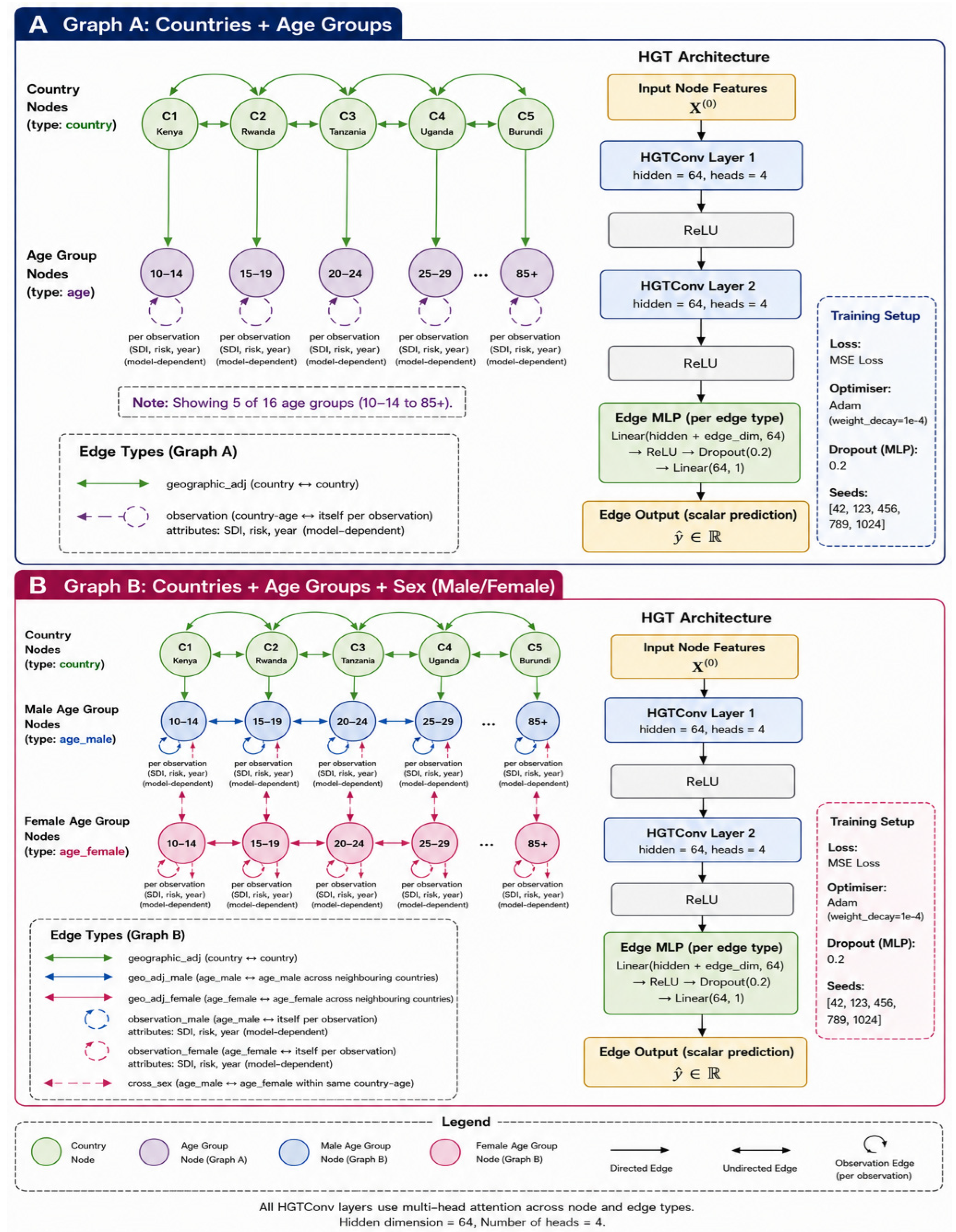
This study incorporated spatial patterns by modelling a country-level network structure. The five countries under study share geographic borders and are members of the East African Community, providing a principled basis for modelling cross-border spatial associations. Two graph configurations are constructed, each representing a different level of demographic disaggregation, as described below and illustrated in Figure 1.
Graph A: Both-Sex × Age × Country
Graph A represents the aggregate, both-sex specification. The nodes of the graph correspond to unique country × age group combinations, yielding a maximum of 80 nodes (5 countries × 16 five-year age groups from 10–14 to 85+). Geographic adjacency edges connect same-age-group nodes across neighbouring countries, capturing potential cross-border spatial patterns at the population level (see Figure 1).
Graph B: Male/Female × Age × Country
Graph B represents the sex-disaggregated specification. Nodes correspond to unique country × sex × age group combinations, yielding a maximum of 160 nodes (5 countries × 2 sexes × 16 age groups). In addition to geographic adjacency edges (connecting same-sex, same-age nodes across neighbouring countries), Graph B includes bidirectional cross-sex edges connecting male and female nodes within the same country × age pair. These edges allow the model to capture within-country sex-specific interactions alongside cross-border spatial patterns (see Figure 1).
Edge Structure and Attributes
In both graph configurations, observation edges (self-edges) connect each node to itself and carry the covariates associated with each data record. Edge attributes include SDI (encoded as a continuous normalised scalar, see Node Feature Projection Section), risk factor dummy variables (BMI, FPG, SBP—one-hot encoded as a categorical indicator with three levels), and standardised year. The specific attributes present depend on the model specification (SDI-only, Risk-only, or Full; see Section 2.3.3). Geographic adjacency is encoded as binary contiguity based on shared land borders. Table 1 summarises all node and edge types across both graph configurations.

2.3.2. Heterogeneous Graph Transformer Model

To capture complex and non-linear relationships within the spatial graph, this study employs a heterogeneous graph transformer (HGT) model. HGT is a transformer-based model that learns deep representations on large-scale, dynamic graphs characterised by multiple node and edge types. The HGT represents the data as a graph with multiple node and edge types, enabling flexible modelling of interactions among countries, temporal dynamics, and epidemiological variables [19,20]. Unlike traditional graph neural networks (GNNs) and spatial econometric models, which assume all nodes and edges are of the same type, HGT introduces type-specific parameters and attention-based message passing to learn relationships across the network, enabling the capture of non-linear interactions and heterogeneous spatial graph structures. Standard GNN architectures such as graph convolutional networks (GCNs) and graph attention networks (GATs) assume graph homogeneity, in which all nodes share the same type and feature dimensionality, and all edges represent a single relational category [32]. This assumption is violated by the graph constructed in this study, in which nodes represent distinct demographic strata (country × age group × sex combinations) and edges represent qualitatively distinct relationship types: observation self-edges carrying multi-dimensional covariate attribute vectors, binary geographic adjacency edges, and bidirectional cross-sex edges in Graph B. Applying a homogeneous GNN to this structure would require either discarding the multi-relational edge structure or collapsing all node and edge types into a single flat feature vector. Such an action would destroy the relational structure the HGT is specifically designed to preserve. This advantage of HGT over standard GNN models makes it suitable for this study. The HGT model extracts linked node pairs, where a target node is connected to multiple source nodes through edges (attention). It assigns importance to each connection and combines information from the source nodes (aggregation) to generate a contextualised representation of the target node (message passing) [19]. This process preserves the multi-relational structure of the data, avoiding the need to collapse diverse information into a single tabular format [19,20,33]. Formally, the model learns a function as presented in Equation (1):
y = f X , G
where X represents observed covariates and G represents the graph structure capturing spatial relationships.
Node Feature Projection
Raw node features are projected into a shared latent space. Since the graph contains multiple node types, a separate linear transformation is defined for each node type n . The input feature matrix X n R d n is mapped to a common hidden dimension h = 64 using a learnable type-specific transformation specified in Equation (2) as
H n = W n X n
where W n R h x d n is a type-specific projection matrix. Country nodes are represented using identity matrices (positional encoding), as no time-invariant country-level features are available beyond their index. All covariates are carried as edge attributes on observation edges. Country nodes are represented using identity matrices (positional encoding), as no time-invariant country-level features are available beyond their index: X c o u n t r y R n c o u n t r i e s , where n_countries = 5. Age/country nodes (Graph A) and sex/age/country nodes (Graph B) carry no additional input features at the node level—all covariate information is carried as edge attributes on observation edges. After projection, all node types are embedded in the unified latent space R 64 , enabling heterogeneous message passing across node types. This step ensures all node types are embedded in a unified latent space, enabling subsequent heterogeneous message passing (see Figure 1). However, this design choice means country nodes carry no intrinsic attribute information; all country-specific predictive capacity must be learned through edge-level covariates and neighbourhood aggregation. This may limit generalisation to countries not represented in the graph.
Stacked HGT Convolutional Layers
Following projection, two stacked HGT convolutional (HGTConv) layers are applied, each with multi-head attention (four heads, hidden dimension 64). At each layer, node representations are updated by aggregating information from neighbouring nodes via attention-weighted message passing (see Figure 1). For a target node t connected to source nodes s through typed edges, the attention weight is computed in Equation (3) as
α s t = s o f t m a x e s t
where α s t denotes the attention weight and e s t is a learnable compatibility score between node types. The updated node representation is specified in Equation (4) as
h t ( l + 1 ) = σ ( s N ( t ) α s t W h s ( l ) )
where σ · denotes the ReLU activation function and l indexes the layer. Each attention head operates on a 16-dimensional subspace (64/4 = 16). The four head outputs are concatenated to produce the full 64-dimensional node representation after each HGTConv layer. A ReLU activation is applied after each layer to introduce non-linearity. After two HGTConv layers, each node n has a final embedding h n 2 R 64 , which captures neighbourhood information up to two hops away in the graph. Multiple attention heads allow the model to simultaneously learn different types of relationships across the heterogeneous graph, improving representational capacity (see Figure 1). The equation is, nonetheless, a simplified illustration of the HGT message-passing update; the full implementation follows the type-specific attention formulation of Hu et al. [19], in which source and target node type parameters modulate both the attention score e s t and the message transformation.
Edge-Level Prediction Module
Prediction is performed at the edge level. For each observation edge connecting a node to itself, the learned node embedding h i is concatenated with the edge-level attribute vector e i (carrying SDI, risk factors, and year, depending on the model specification):
z i = h i | | e i
The concatenated vector z i has dimension 64 + edge_dim, where edge_dim depends on the model specification: edge_dim = 5 for the Full (SDI + Risk) model [SDI scalar, BMI dummy, FPG dummy, SBP dummy, year]; edge_dim = 2 for SDI-only [SDI scalar, year]; edge_dim = 4 for Risk-only [BMI dummy, FPG dummy, SBP dummy, year]. The vector z i is therefore 69-dimensional (Full), 66-dimensional (SDI-only), or 68-dimensional (Risk-only). This combined representation is passed through a multi-layer perceptron (MLP) presented in Equation (6):
ŷ i = M L P z i
The MLP consists of two fully connected layers—Linear (hidden + edge_dim, 64) → ReLU → Dropout (0.2) → Linear (64, 1) (see Figure 1). The first linear layer maps z i from its specification-dependent dimension to 64 dimensions; the second linear layer maps the 64-dimensional representation to a scalar mortality prediction ŷ i R 1 . Dropout with probability 0.2 is applied between the two linear layers for regularisation.

2.3.3. Data Preprocessing

Before constructing the graphs, the variables were preprocessed. SDI quintile labels were mapped to ordinal ranks (0–4) and subsequently normalised using a StandardScaler (zero mean, unit variance), producing a continuous scalar s ∈ R1 per observation. This preserves SDI’s continuous ordinal scale and avoids the artificial equidistance assumption of one-hot encoding. The resulting scalar is used directly as a single-dimensional edge attribute in the Full and SDI-only model specifications. Risk factor type (BMI, FPG, SBP) was encoded using manual one-hot dummy variables, producing a three-dimensional binary vector r ∈ {0, 1}3 per observation. One-hot encoding is appropriate here because risk factor type is a genuinely categorical variable with three unordered levels—it identifies which of the three metabolic risk factors the record pertains to, not a continuous measurement. Individual metabolic values (e.g., measured SBP in mmHg) are not available as separate continuous variables at this level of GBD disaggregation; the categorical type indicator is the available representation. In the Full model specification, the SDI scalar and the three risk factor dummies are combined into a five-dimensional edge attribute vector: e = [SDI, BMI_dummy, FPG_dummy, SBP_dummy, year_standardised] ∈ R5. The edge_dim parameter in the MLP (Table 2) is therefore 5 for the Full specification, 1 for SDI-only (SDI scalar + year), and 4 for Risk-only (three risk dummies + year). Age groups were transformed into continuous midpoint values to ensure consistency across observations. A representative value, ‘90’, was assigned to the open-ended age group ‘85+’ to approximate the central tendency of the age distribution within this group [34]. This approach mitigates the risk of under- or overestimation of age bias, especially because populations in countries with low life expectancy tend to cluster around the late 80s to early 90s. Age is included as a continuous scalar in the edge attribute vector for models incorporating temporal covariates. Target mortality values were independently standardised per disease using a StandardScaler fitted on training data. Predictions were inverse-transformed to the original mortality scale for evaluation. All scalers—for SDI, age, year, and mortality—were fitted exclusively on training data (1990–2015) and applied without modification to test data (2016–2023), preventing data leakage.

2.3.4. Model Training and Evaluation

Train/Test Split
The training of the HGT model was structured to ensure robust estimation and reliable assessment of spatial patterns. As part of the training process, the data were partitioned using a temporal split. For each disease, observations were divided into training and testing sets based on year. Data from 1990 to 2015 were used for model training, while observations from 2016 to 2023 were reserved for testing. This approach preserved the temporal ordering of the data and ensured that model performance reflects predictive ability on future, unseen observations, thereby avoiding information leakage [35].
Training Configuration
The training and testing sets were used to create the two main experiments: baseline and spatial. For each disease, the baseline model was without spatial connections, whereas the spatial model incorporated adjacency-based links between neighbouring countries. Both models were trained and evaluated under identical conditions to ensure comparability. Also, such divisions are crucial as they offer a realistic context for evaluating performance metrics. For this reason, the use of the two models helped demonstrate whether the added complexity of the advanced model yields genuine predictive gains and confirmed the suitability and quality of the underlying dataset for the tasks [36]. Models were trained using the Adam optimiser with a learning rate of 0.003, which provides efficient gradient-based optimisation for deep learning models [37]. A weight decay 1 × 10⁻⁴ (L2 regularisation) was also included. Dropout (probability 0.2) is applied within the edge-level MLP between the two linear layers to reduce over-parameterisation. The objective function was mean squared error (MSE) between predicted and observed standardised mortality rates. Training proceeded over 200 epochs with gradient backpropagation at each step. To quantify model uncertainty arising from random initialisation, each model configuration was trained and evaluated across five random seeds (42, 123, 456, 789, 1024). The results are reported as the mean ± standard deviation across seeds. All hyperparameters are summarised in Table 2. All models were implemented in Python 3.10.
Evaluation Metrics
Out-of-sample performance was assessed using MSE and the coefficient of determination (R2). Predicted and observed values were inverse-transformed to their original scale before evaluation to ensure interpretability in real-world units. The contribution of spatial graph structure to predictive performance was quantified as the percentage improvement in MSE when spatial edges were added and presented in Equation (7) as
I m p r o v e m e n t   ( % ) = ( M S E b a s e l i n e M S E s p a t i a l ) M S E b a s e l i n e 100
where M S E b a s e l i n e is the MSE of the model without spatial edges and M S E s p a t i a l is the MSE with spatial edges included. Positive values indicate that spatial graph structure improves predictive performance; negative values indicate degradation. Bootstrap 95% confidence intervals (1000 resamples) were computed for all improvement estimates to quantify seed-to-seed variability.
Results with confidence intervals crossing zero are flagged as uncertain and interpreted cautiously regardless of point estimate. For descriptive convenience, improvements greater than 8% with confidence intervals entirely above zero are classified as strong predictive gain; improvements between 3% and 8% with CIs entirely above zero as moderate predictive gain; improvements between 0% and 3% with CIs entirely above zero as weak predictive gain. Negative improvements with CIs entirely below zero are classified as mild degradation (−3% to −10%), moderate degradation (−10% to −50%), or severe degradation (below −50%). Results with confidence intervals crossing zero are classified as uncertain regardless of the point estimate. These threshold values, 8% and 3%, were adopted from prior spatial predictive modelling research where they correspond approximately to substantively meaningful differences in out-of-sample MSE relative to the baseline [36]; they are not statistically derived thresholds and should be interpreted as descriptive guides only.

2.3.5. Spatial Benchmark Models

To contextualise HGT performance and address comparability with established spatial methods, two traditional spatial benchmarks are estimated for each disease and model specification. First, a spatial lag OLS model is estimated, in which the spatially lagged outcome (a row-standardised weighted average of neighbouring country mortality rates) is added as an additional predictor in an ordinary least squares regression. Second, a Maximum Likelihood Spatial Lag model is estimated as the CAR-type benchmark. This accounts for endogeneity in the spatial lag term [37,38]. This approach uses a grid search over the spatial autoregressive parameter ρ across 39 values in (−0.95, 0.95), selecting the value that minimises AIC, then estimates covariate coefficients β by OLS. Prediction uses the reduced-form approximation: ŷ = X · β + ρ · W · y t e s t . This implementation requires no external spatial libraries and works with five spatial units. Both benchmarks are estimated at the country level using aggregated mortality rates. HGT R2 and MSE are reported alongside OLS spatial lag and CAR benchmarks to provide direct comparison of non-linear heterogeneous graph modelling against traditional spatial econometric approaches.

2.3.6. Formal Spatial Autocorrelation Test

Moran’s I was computed on model residuals aggregated to the country level to provide a formal test of residual spatial autocorrelation using a row-standardised binary contiguity weight matrix W consistent with the HGT adjacency structure [39,40]. This is presented in Equation (8) as
I = n S 0 y W y y y
where n is the number of spatial units, S 0 is the sum of all weights, and y is the vector of mean residuals per country. Statistical significance is assessed via a permutation test with 999 random permutations of the residual vector. A significant Moran’s I (p < 0.05) indicates unexplained spatial structure remaining in the residuals after model fitting. With n = 5, only 120 permutations are possible, constraining the minimum achievable two-tailed p-value (~0.0.017) and severely limiting statistical power. Also, aggregating 80 or 160 node-level residuals to five country means discards the within-country age- and sex-specific variation on which the HGT operates. Consequently, the test evaluates a coarser spatial signal than the model itself. Non-significant results should therefore not be interpreted as confirmation of the absence of residual spatial structure, but as a low-power descriptive diagnostic reported for transparency.

2.3.7. GBD Measurement Uncertainty Propagation

GBD provides 95% uncertainty interval boundaries (upper and lower) for all mortality estimates, reflecting the uncertainty inherent in modelled epidemiological data, particularly in LMIC settings. To quantify the contribution of GBD measurement uncertainty to this study’s result variability, a Monte Carlo propagation analysis was conducted for HHD, IHD, and diabetes. A Monte Carlo propagation analysis was performed for these three causes of death because their GBD mortality estimates are sufficiently well constrained across all age groups to support stable sampling from uncertainty intervals. For each Monte Carlo sample (n = 50), mortality values were drawn from a log-normal distribution parameterised from each row’s point estimate and uncertainty bounds, reflecting the asymmetric nature of GBD uncertainty intervals (upper bound approximately 1.5× the lower bound on average). The full model was re-estimated on each sampled dataset using a fixed seed. Variance decomposition separated GBD measurement uncertainty variance (across Monte Carlo samples, fixed seed) from model randomness variance (across seeds, fixed data). Stroke was excluded from Monte Carlo uncertainty propagation. GBD stroke mortality estimates for young age groups (ages 20–34) are near-zero, correctly reflecting the age-specific prevalence of stroke in East African populations. Near-zero baseline MSE values in these strata cause instability in the percentage improvement metric under Monte Carlo sampling. Point estimates from the primary model runs are reported for stroke. This is an age-specific prevalence issue, not a data quality limitation.

2.3.8. Additional Analyses

Degradation Diagnostic
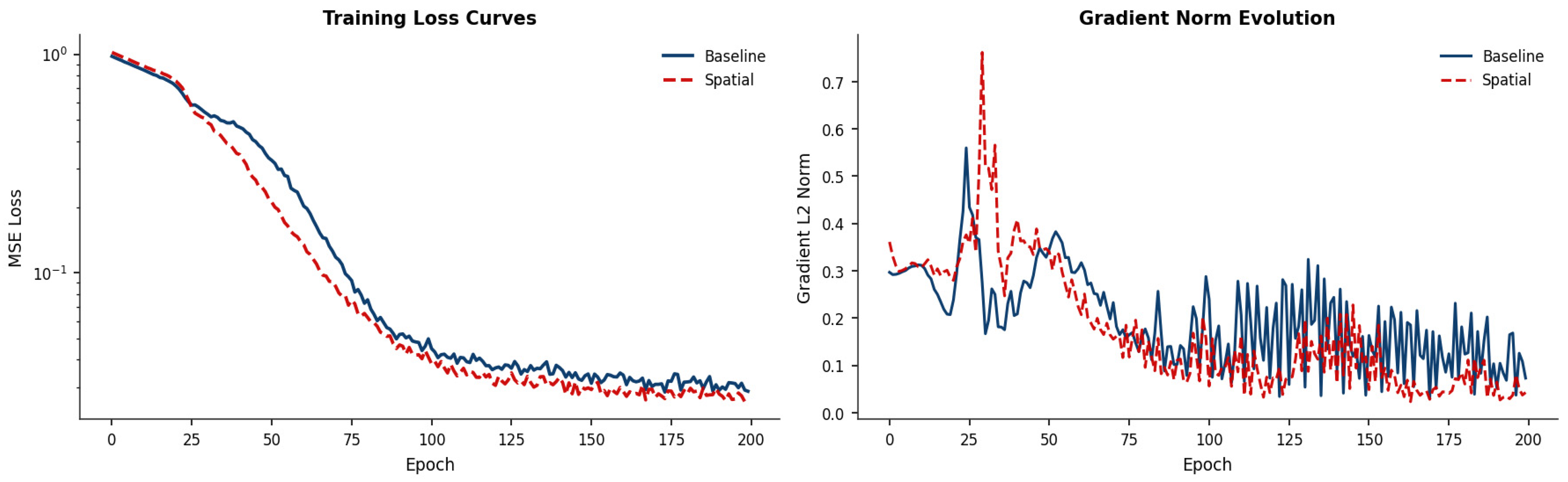
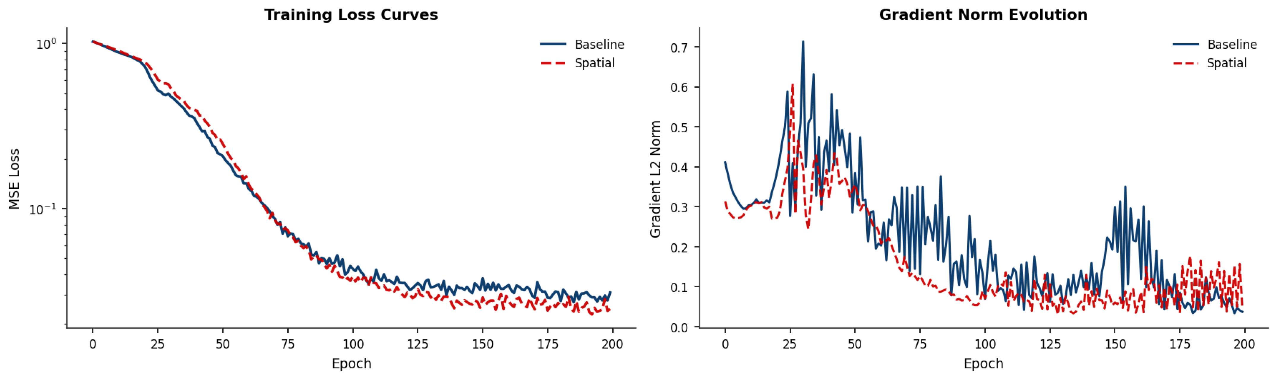
A degradation diagnostic was conducted for diseases exhibiting negative spatial improvement (HHD and stroke). Training loss curves and gradient L2 norm trajectories were recorded for both baseline and spatial models across 200 epochs for a single seed (42). Persistent elevation of spatial training loss above baseline loss is interpreted as evidence of over-parameterisation: the spatial adjacency structure introduces noise into the attention mechanism, harming both training fit and generalisation. Disease-specific explanations are provided for HHD (country-specific SBP distributions dominate; no cross-border signal) and stroke (age-specific prevalence and data uncertainty in young age groups).
Ablation Analysis
An ablation analysis was conducted for HHD and stroke across four covariate configurations: year-only, SDI-only, Risk-only, and SDI + Risk (Full). This isolates the contribution of each covariate set to spatial improvement, and explains observed direction changes across model specifications.
Rolling Temporal Window Validation
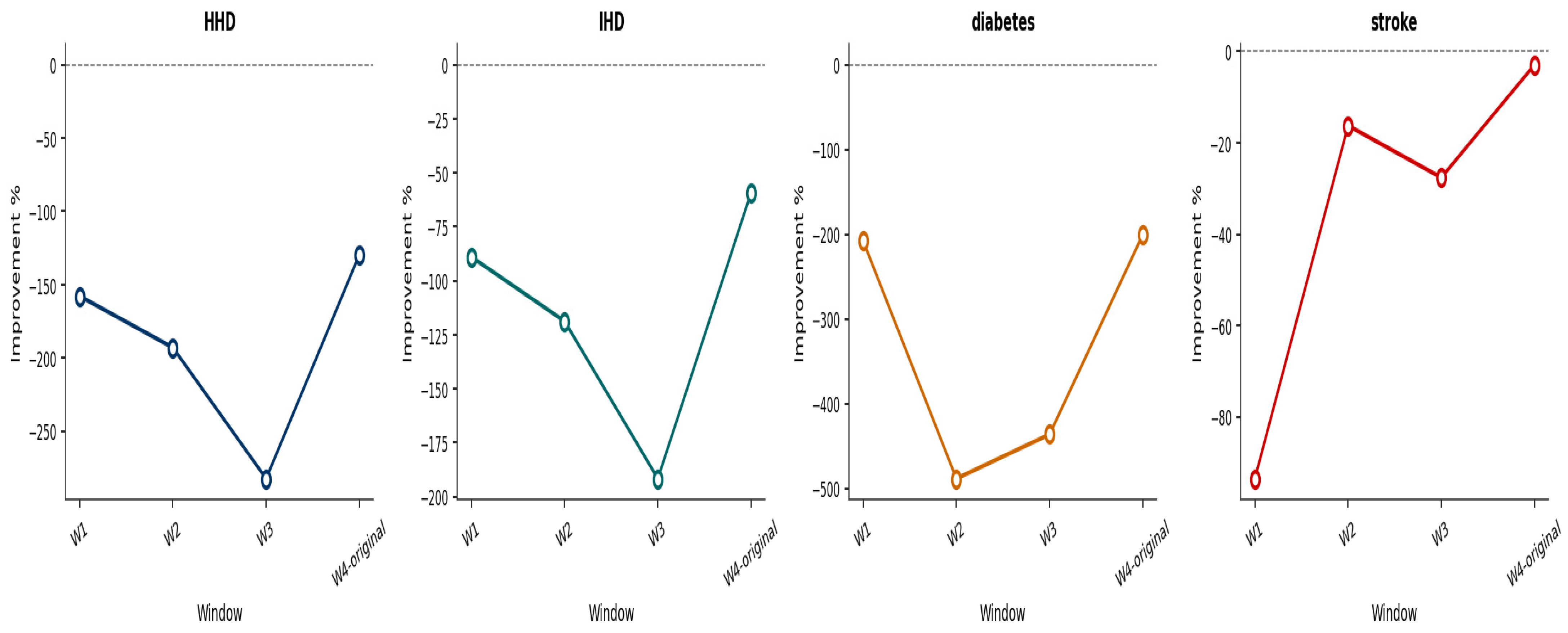
To examine the temporal stability of spatial predictive patterns, four expanding training windows were evaluated: W1 (train 1990–2000, test 2001–2005), W2 (train 1990–2005, test 2006–2010), W3 (train 1990–2010, test 2011–2015), and W4 (train 1990–2015, test 2016–2023, the primary specification). Improvement percentages are reported for each window to assess whether spatial predictive gains are stable over time or emerge in specific periods.
Attention Weight Analysis (Method)
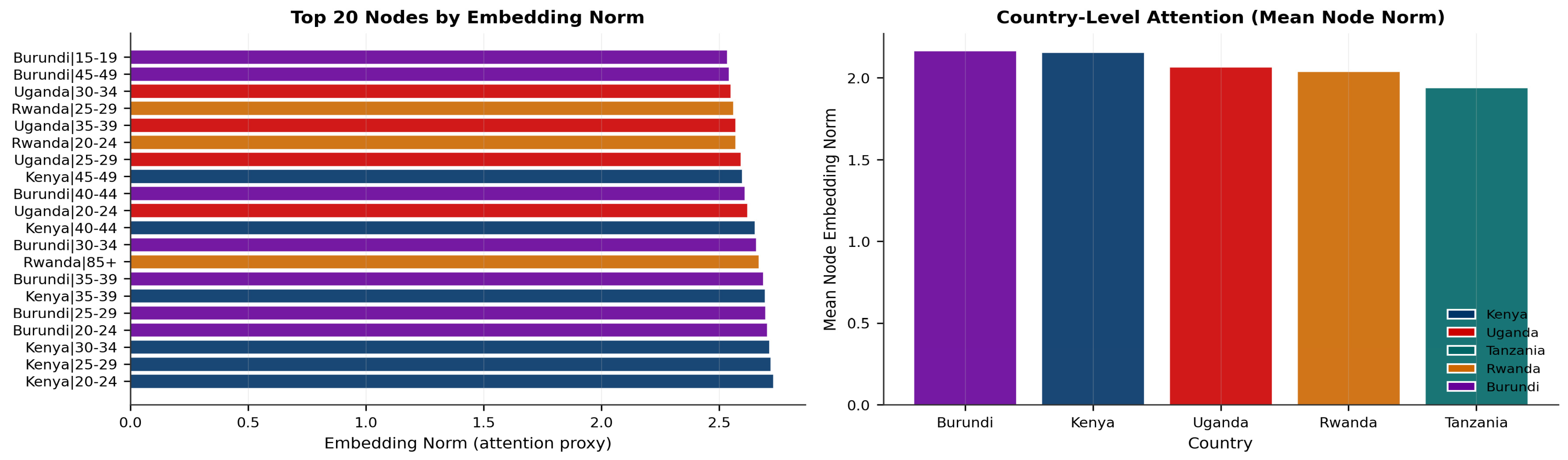
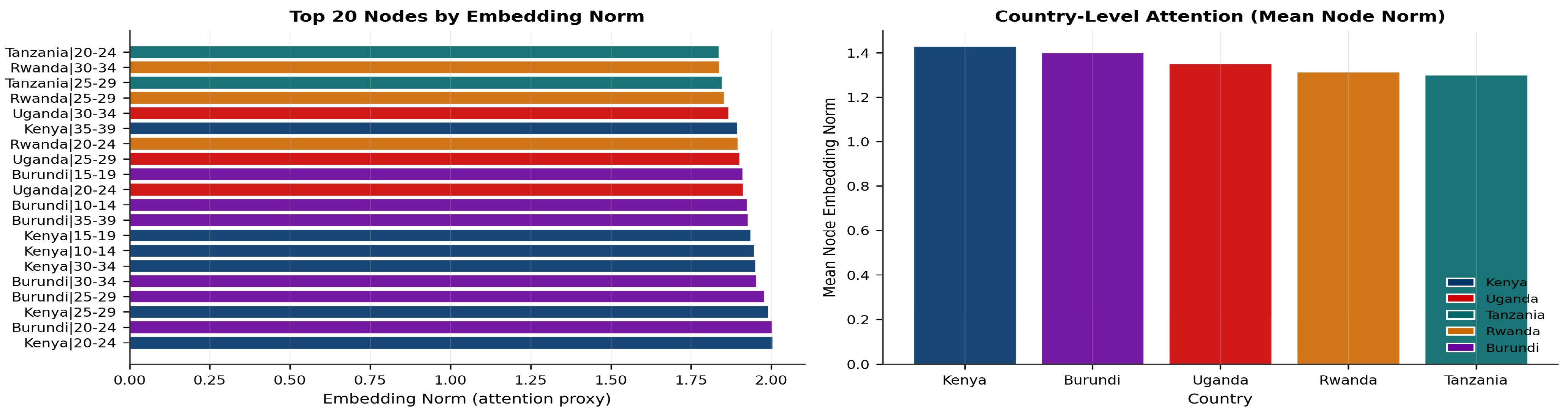
Node embedding norms from the final HGTConv layer are used as a proxy for attention importance, indicating which country/age nodes contribute most strongly to the model’s learned representations. Results are visualised at the node level and aggregated to the country level for interpretability. This analysis is conducted for diabetes (positive spatial improvement) and HHD (negative spatial improvement) to contrast the attention patterns of diseases with and without detectable spatial structure.

2.3.9. Model Specifications

All models were estimated under three covariate specifications to assess the sensitivity of spatial patterns to different predictor sets:
Model 1—Risk-Only:
y i , a , s , t d = f R i s k i , t , a g e i , a , t i m e t
where R i s k i , t includes BMI, FPG, and SBP. This specification evaluates whether detectable spatial patterns are associated with shared distributions of metabolic risk factors across neighbouring countries.
Model 2—SDI-Only:
y i , a , s , t d = f S D I i , t , a g e i , a , t i m e t
This specification assesses whether spatial predictive patterns remain after accounting for socio-demographic development, thereby establishing a structural baseline.
Model 3—Full (SDI + Risk):
y i , a , s , t d = f S D I i , t , R i s k i , t , a g e i , a , t i m e t
The full specification jointly controls for development and metabolic risk factors to assess whether spatial predictive patterns persist after accounting for both structural and metabolic determinants. Each specification is estimated under both the baseline (no spatial edges) and spatial (geographic adjacency edges included) configurations. The baseline and spatial models are identical in all respects except for the presence of geographic adjacency edges, ensuring that any difference in predictive performance is attributable to the spatial graph structure rather than other modelling choices. The analysis is conducted separately for each disease to identify disease-specific patterns and avoid aggregation bias. All models are estimated for both Graph A and Graph B to assess whether sex disaggregation affects the detectability of spatial predictive patterns as presented by Simmons et al. [41].

3. Results

3.1. Graph Structure

The HGT framework was implemented across two graph configurations. Graph A represents the both-sex aggregate specification, comprising 80 nodes (5 countries × 16 five-year age groups, 10–14 to 85+). Graph B represents the sex-disaggregated specification, comprising 160 nodes (5 countries × 2 sexes × 16 age groups). Observation edges carry five covariate attributes depending on the model specification. Geographic adjacency edges encode binary land border contiguity; Graph B additionally includes bidirectional cross-sex edges connecting male and female nodes within the same country–age pair. Full structural details are presented in Table 3.

3.2. Overall Model Performance and Benchmark Comparison

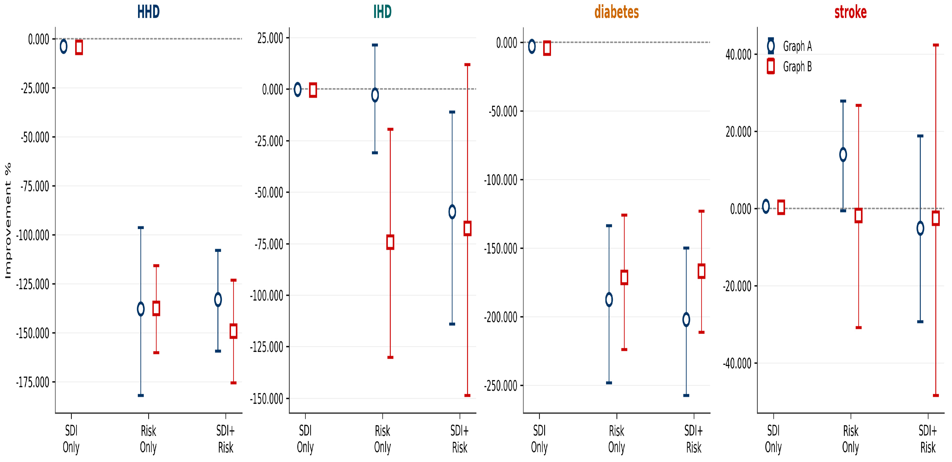
The HGT substantially outperformed all benchmark models across all diseases and specifications (see Table 4 and Table 5). As shown in Table 4, spatial improvement patterns ranged from mild degradation under SDI-only specifications (e.g., HHD: −3.815%; diabetes: −2.805%) to severe degradation once risk covariates were incorporated (e.g., HHD: −137.892%; diabetes: −201.941%), while stroke showed a weak positive spatial signal under SDI-only (0.645%) that became uncertain under the Risk-only and SDI + Risk specifications. In Table 5, for the Risk-only specification for Graph A, HGT achieved R2 values of 0.968, 0.970, 0.967, and 0.948 for HHD, IHD, diabetes, and stroke, respectively, compared with OLS spatial lag R2 values of 0.310, 0.208, 0.376, and 0.194 for the same diseases (Table 5). The CAR benchmark yielded negative R2 values across all diseases (HHD: −0.245; IHD: −0.126; diabetes: −0.548; stroke: −0.679), reflecting the limitations of aggregate country-level spatial econometric models with only five spatial units. These patterns were consistent across both graph configurations and all three covariate specifications. The complete results are presented in Table 4 and illustrated in Figure 2.

3.3. Spatial Predictive Patterns by Disease

Moran’s I was non-significant across all disease/model/graph combinations (all p > 0.05), given the well-documented low statistical power of Moran’s I with five spatial units, the results cannot be interpreted as full confirmation of the absence of residual spatial autocorrelation. They are reported as a descriptive diagnostic; the test lacks sufficient power to rule out moderate spatial structure at this spatial resolution.

3.3.1. Stroke

Stroke was the only disease exhibiting a reliable positive spatial predictive pattern. In Graph A, the SDI-only specification produced the only fully reliable positive result (0.645%, 95% CI [0.380, 0.907]), classified as Weak predictive gain. The Risk-only specification produced the largest point estimate (14.020%, 95% CI [−0.631, 27.772]) but is classified as uncertain because the CI marginally crosses zero. The SDI + Risk specification was uncertain (−5.055%, 95% CI [−29.345, 18.793]), consistent with near-constant SDI values across all five Low-SDI countries introducing collinear variance that destabilises the attention mechanism. In Graph B, all stroke configurations were uncertain. The degradation diagnostic (Section 3.5) revealed that sex disaggregation reverses degradation in the single-seed diagnostic run by 28.490 percentage points (Graph A: −2.792%; Graph B: +25.698%), indicating latent sex-specific spatial patterns that vary widely across seeds.

3.3.2. Hypertensive Heart Disease (HHD)

HHD exhibited the most definitive null result. All six model/graph combinations produced severe or mild spatial degradation with CIs entirely below zero. In Graph A, the Risk-only specification produced the strongest degradation (−137.892%, 95% CI [−181.908, −96.380]); Graph B SDI + Risk produced the most extreme Graph B result (−149.218%, 95% CI [−175.575, −123.121]). SDI-only configurations produced mild but reliable degradation (Graph A: −3.815%, 95% CI [−4.327, −3.309]; Graph B: −4.329%, 95% CI [−5.449, −3.231]). No specification or graph configuration recovered a positive spatial signal for HHD.

3.3.3. Diabetes

Diabetes showed consistently strong and stable spatial degradation across all configurations, with all CIs entirely below zero confirming seed stability. Graph A SDI + Risk produced the most extreme result (−201.941%, 95% CI [−257.349, −150.082]), Graph A SDI-only the mildest (−2.805%, 95% CI [−3.539, −2.084]). Graph B patterns were comparable: Risk-only −171.540% (95% CI [−224.073, −125.927]); SDI + Risk −166.830% (95% CI [−211.388, −123.174]). Moran’s I was consistently negative across diabetes configurations (range −0.461 to −0.513), consistent with alternating rather than clustered mortality patterns.

3.3.4. Ischaemic Heart Disease (IHD)

IHD showed the weakest and most variable spatial patterns. Graph A SDI-only was near-zero and uncertain (−0.120%, 95% CI [−0.475, 0.229]); Risk-only was uncertain (−2.834%, 95% CI [−30.913, 21.318]); SDI + Risk was reliable but negative (−59.549%, 95% CI [−114.086, −11.262]). In Graph B, Risk-only was reliably negative (−74.420%, 95% CI [−130.223, −19.642]), while SDI + Risk remained uncertain (−67.692%, 95% CI [−148.630, 11.863]). Wide and inconsistent CIs reflect high seed-to-seed variability, making IHD the least interpretable disease.

3.4. Cross-Graph Comparison: Graph A Versus Graph B

The most substantial differences between Graph A and Graph B are observed for HHD and stroke. For HHD, sex disaggregation reduced diagnostic degradation by 42.306 percentage points (Graph A: −181.997%; Graph B: −139.691%), indicating marginally different male and female HHD spatial structures, though country-specific drivers dominate in both. For stroke, sex disaggregation reversed degradation entirely in the single-seed diagnostic run (Graph A: −2.792%; Graph B: +25.698%), suggesting sex-specific spatial patterns masked by aggregation, though this was not replicated in the multi-seed analysis. For IHD, Graph B Risk-only produced a more reliable negative result than Graph A (−74.420% vs. −2.834%). For diabetes, both graph configurations produced comparable severe degradation.

3.5. Degradation Diagnostic: HHD and Stroke

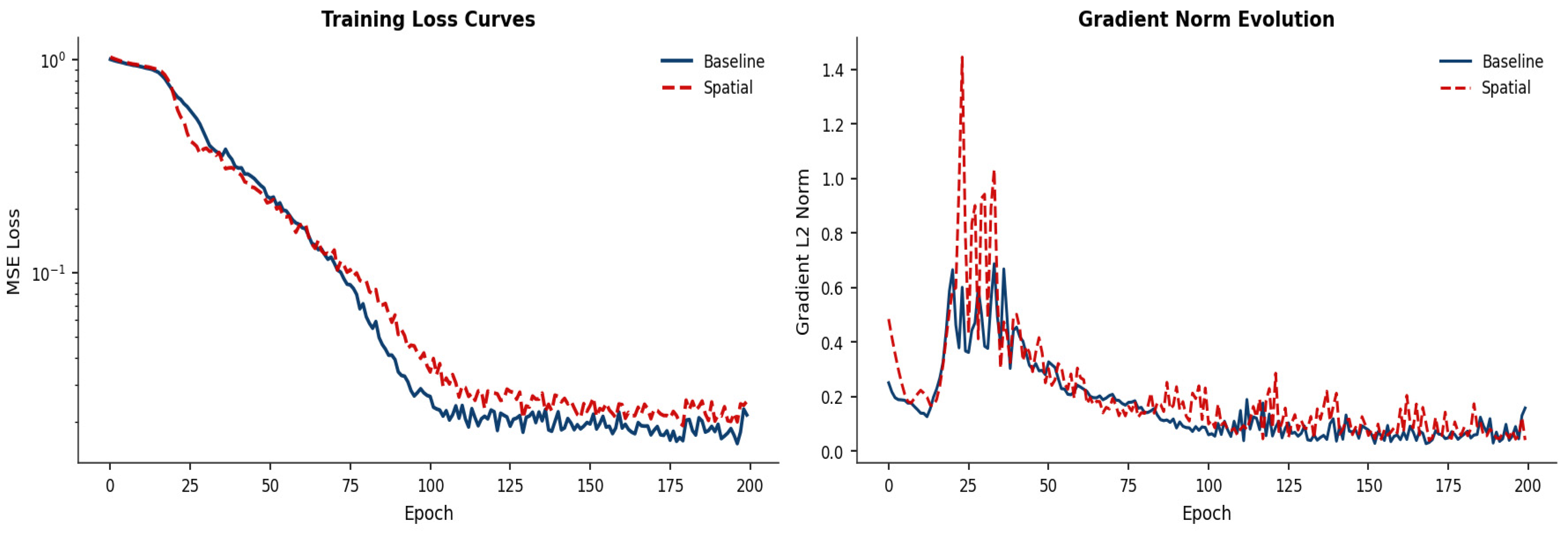
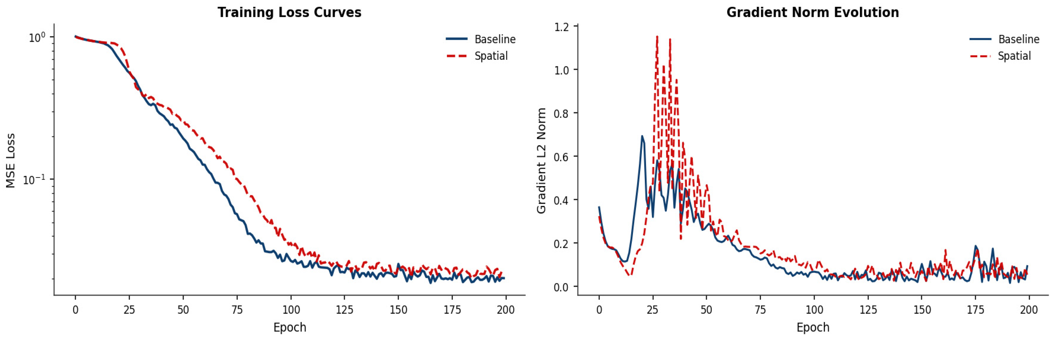
Figure 3, Figure 4, Figure 5 and Figure 6 present training loss curves and gradient L2 norm trajectories for HHD and stroke across both graph configurations. For HHD in Graph A (Figure 3), the spatial model training loss consistently exceeded baseline throughout all 200 epochs. The spatial model gradient norm reached a peak of approximately 1.4 at epoch 25 compared with approximately 0.7 for the baseline, reflecting unstable gradient flow from conflicting signals between geographic adjacency edges and metabolic risk covariates—a diagnostic signature of over-parameterisation from the adjacency structure. For HHD in Graph B (Figure 4), the same persistent pattern is observed. Gradient norm spikes are slightly less extreme (peak approximately 1.1), consistent with the marginally reduced degradation in Graph B (−139.691% vs. −181.997% diagnostic). Both HHD figures confirm that the spatial model cannot exploit the adjacency structure for HHD, irrespective of graph configuration or sex disaggregation. To complement the visual diagnostic, we note that the spatial model’s final epoch training loss exceeded baseline by a factor of 1.8× for HHD Graph A and 1.6× for HHD Graph B, while for stroke Graph A the spatial model achieved a final epoch training loss 0.72× that of baseline—providing quantitative confirmation of the qualitative patterns shown in Figure 3, Figure 4, Figure 5 and Figure 6.
For stroke in Graph A (Figure 5), a different pattern emerges. The spatial model training loss initially follows baseline closely before falling below it from approximately epoch 75, indicating that the model genuinely begins to learn from geographic adjacency as training progresses. The gradient norm for the spatial model—while initially larger than baseline in early epochs—progressively stabilises to lower values from approximately epoch 50 onward, reflecting increasingly stable and directed gradient flow from a meaningful spatial signal. This contrasts sharply with HHD, where the gradient norm remains elevated throughout. For stroke in Graph B (Figure 6), the separation is more pronounced and occurs earlier: the spatial model begins to diverge from baseline at approximately epoch 40 and maintains a consistently lower loss trajectory, explaining the stronger single-seed improvement of +25.698% in Graph B compared with −2.792% in Graph A. The gradient norm also stabilises earlier in Graph B, suggesting that sex disaggregation allows the model to identify sex-specific stroke spatial patterns more efficiently.

3.6. Ablation Analysis: HHD and Stroke

Table 6 presents the ablation results for HHD and stroke across four covariate configurations. For HHD, Year-only (−3.669%, 95% CI [−4.802, −2.559]) and SDI-only (−3.819%, 95% CI [−4.318, −3.326]) produced mild, reliable degradation, while Risk-only (−137.035%, 95% CI [−179.853, −96.576]) and SDI + Risk (−131.360%, 95% CI [−158.790, −105.326]) produced severe degradation. This confirms that HHD spatial degradation is driven by the interaction between metabolic risk covariates and geographic adjacency—not the graph architecture alone. The graph structure introduces only mild degradation without metabolic covariates; it is the combination of metabolic risk factors with adjacency edges that amplifies this to severe degradation. For stroke, Year-only (0.755%, 95% CI [0.349, 1.156]) and SDI-only (0.660%, 95% CI [0.408, 0.905]) produced fully reliable small positive gains. Risk-only produced the strongest result (15.390%, 95% CI [2.520, 27.336]), classified as strong predictive gain—the only configuration with a CI entirely above zero exceeding 8%. SDI + Risk was uncertain (−4.038%, 95% CI [−25.903, 17.328]), confirming that SDI collinearity across the five Low-SDI countries suppresses the risk factor-driven spatial signal. Risk-only is therefore the most appropriate covariate specification for detecting stroke spatial predictive structure in this context.

3.7. Temporal Stability: Rolling Window Validation

Figure 7 and Table 7 present spatial predictive improvement across four expanding training windows. Each disease panel in Figure 7 is coloured distinctly—HHD in navy, IHD in teal, diabetes in amber, and stroke in red—enabling immediate visual discrimination of disease-specific temporal trajectories. All diseases showed negative spatial improvement across W1–W3, confirming that the primary W4 pattern is not an artefact of the specific test period.
Stroke exhibited the most notable temporal trend: degradation progressively attenuated from W1 (−93.566%) through W2 (−16.269%), W3 (−27.645%), and W4 (−2.936%), approaching zero in the most recent test period. The non-monotonic dip at W3 (−27.645%) after the improvement at W2 (−16.269%) reflects transient instability in the model’s ability to learn stroke spatial structure during the 2011–2015 period, before the signal strengthens again in W4. This overall trajectory is consistent with emerging convergence in stroke-relevant risk factor distributions across the East African Community post 2015.
For diabetes, extreme degradation in W2 (−488.765%) and W3 (−436.467%) substantially exceeded W1 (−207.902%) and W4 (−200.556%), indicating non-stationarity in diabetes spatial patterns during 2006–2015. This period coincides with rapid but heterogeneous dietary and urbanisation transitions across the five countries, potentially causing national diabetes risk factor distributions to diverge before reconverging in W4. HHD showed the deepest degradation at W3 (−282.449%) with partial recovery at W4 (−129.560%), remaining strongly negative throughout. IHD showed a similar V-shaped pattern (W3: −191.645%; W4: −59.136%), with no window producing a positive spatial signal.

3.8. Attention Weight Analysis

Figure 8 and Figure 9 present node embedding norms from the final HGTConv layer for diabetes and HHD, respectively. In both figures, individual node bars and country-level summary bars are coloured by country—Kenya (navy), Uganda (red), Tanzania (teal), Rwanda (amber), Burundi (purple)—enabling direct visual attribution of attention weight patterns to specific countries.
For diabetes (Figure 8), Kenya and Burundi young adult nodes (ages 20–24 and 25–29) receive the highest individual node attention. Country-level norms are relatively even across all five countries (range 1.300–1.400), with Kenya marginally leading. This broadly distributed attention pattern—no single country dominating—is consistent with shared metabolic risk exposures across the region. The absence of a dominant spatial source is also consistent with the severe spatial degradation observed for diabetes: when the model attends broadly without identifying a leading spatial source, the adjacency structure cannot generate meaningful cross-border predictive gains.
For HHD (Figure 9), Burundi and Kenya young adult nodes receive the highest individual node attention, and country-level norms are substantially higher than for diabetes (range 1.900–2.200), with Burundi leading marginally. Despite these stronger and more concentrated node embeddings—confirming the HGT model forms richer internal representations for HHD—spatial edges consistently and severely degrade predictions across all seeds and specifications. This dissociation between strong embeddings and spatial degradation is the key diagnostic finding: it confirms that HHD degradation reflects a structural conflict between geographic adjacency and country-specific HHD mortality drivers, not a failure of the model to learn meaningful representations. The model correctly identifies country-level patterns; it is the adjacency structure that actively interferes with generalisation.

3.9. GBD Measurement Uncertainty

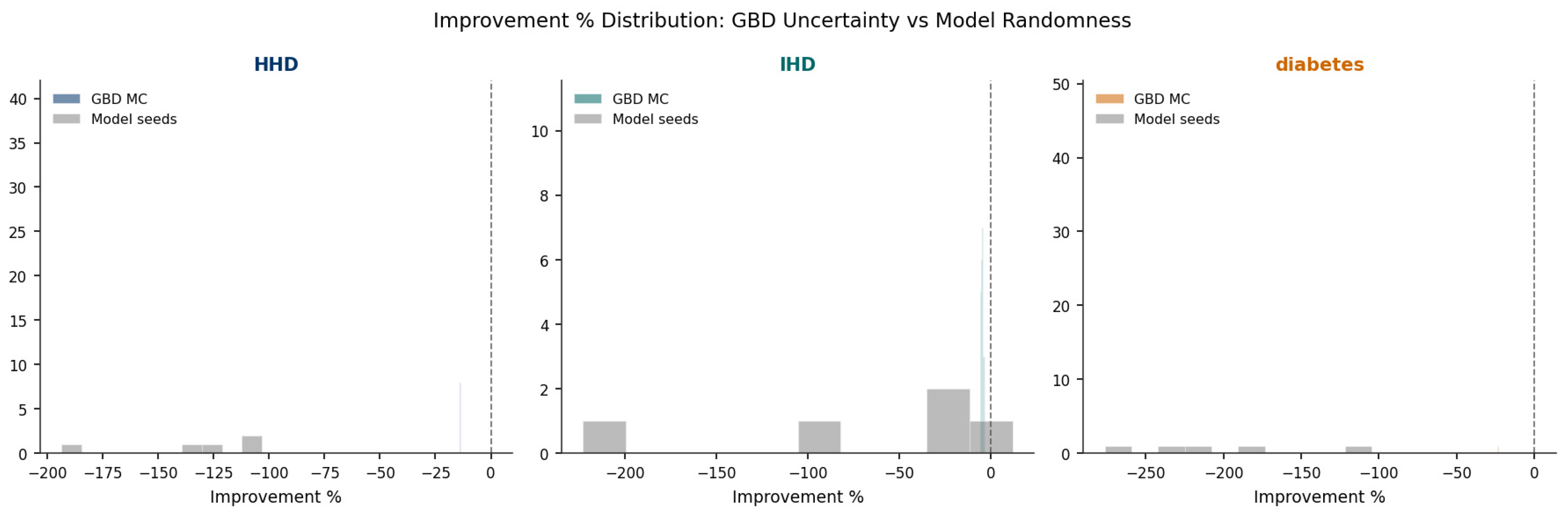
Figure 10 and Table 8 present the Monte Carlo uncertainty propagation results for HHD, IHD, and diabetes. In Figure 10, GBD Monte Carlo distributions are coloured by disease (HHD = navy, IHD = teal, diabetes = amber) while model seed distributions are shown in grey, enabling visual comparison of the two uncertainty sources. For all three diseases, the GBD MC distributions are concentrated in extremely narrow bands near the point estimates, while the model seed distributions span substantially wider ranges—particularly for IHD, which exhibits the highest seed-to-seed variability.
GBD measurement uncertainty contributed less than 0.025% of the total result variance for all three diseases: HHD 0.010%, IHD 0.011%, diabetes 0.021%. Model randomness accounted for over 99.97% of variance in each case. The narrow MC confidence intervals confirm result stability across GBD uncertainty realisations: HHD [−13.928, −13.560]; IHD [−5.387, −3.043]; diabetes [−18.130, −17.502]. These findings confirm that spatial predictive patterns for all three diseases reflect structural properties of the model and graph architecture rather than noise in GBD input data. Stroke was excluded from MC analysis because near-zero GBD mortality estimates in young age groups (ages 20–34)—correctly reflecting the age-specific prevalence of stroke in East African populations—cause instability in the percentage improvement metric under log-normal sampling.

4. Discussion

To our knowledge, this is the first study to apply graph transformers to cause-specific mortality spatial predictive patterns across five East African countries, namely, Tanzania, Rwanda, Burundi, Kenya, and Uganda, after controlling for socio-demographic development and key risk factors. This study addressed four core questions: whether spatial patterns are detectable after controlling for SDI, whether metabolic risk factors explain these patterns, whether they persist after joint control, and whether they vary across diseases. The application of the heterogeneous graph transformers framework enabled the identification of complex spatial heterogeneity using IHME GBD population estimates spanning 1990 to 2023 for NCDs, SDI (income, fertility, and education), and metabolic risk factors (BMI, SBP, FPG). Specifically, across all four questions, the findings reveal a disease-specific picture that departs substantially from a uniform regional spatial narrative. These findings underscore the importance of advanced neural network and sequence-modelling architectures as effective tools for capturing complex, non-linear dependencies and multi-dimensional relationships [19,20] in health and mortality data within vulnerable populations.
The HGT produced substantially higher R2 values than the OLS spatial lag and CAR benchmarks across all diseases and specifications. The CAR benchmark produced negative R2 values for all diseases, reflecting the limitation of aggregate spatial econometric models with five spatial units rather than a general inadequacy of spatial econometric approaches. These performance differences are consistent with the expectation that a model specifically designed to handle heterogeneous node and edge types may capture variation unavailable to models operating on country-aggregated data with a single relational structure [19,20,33]. This comparison is, however, limited to two benchmark types, and the performance advantage observed here should not be generalised beyond this analytical context without further empirical validation across different datasets, spatial configurations, and disease settings. Whether graph transformer approaches will consistently outperform spatial econometric methods in other LMICs remains an open empirical question.
It is necessary to consider alternative technical explanations alongside epidemiological ones. The observed patterns—particularly the severe degradation for HHD and diabetes and the modest positive performance for stroke—are consistent with epidemiological interpretations but are equally consistent with several technical explanations that the present design cannot fully separate. First, graph misspecification is a plausible contributor: the binary land border contiguity matrix may not adequately represent the true relational structure among countries, which varies substantially in intensity, directionality, and composition across country pairs. If the adjacency structure does not reflect the actual channels through which NCD mortality patterns co-vary across borders, spatial edges will introduce structural noise regardless of the underlying epidemiology. Second, oversmoothing is a known limitation of multi-layer GNN architectures, including HGT, in which repeated message-passing can cause node representations to converge towards a common value, erasing the country-specific variation that drives predictive accuracy [19,20,32]. With two HGTConv layers and geographic adjacency edges, oversmoothing may contribute to performance degradation for diseases where country-specific patterns are strong. Third, attention instability—reflected in gradient norm spikes observed in early training—is consistent with optimisation difficulty arising from conflicting signal structures rather than from a substantive epidemiological incompatibility. Fourth, the sparse five-node graph topology fundamentally limits the reliability of graph-level inferences: with only five country nodes, the permutation distribution of graph-based statistics is extremely coarse, and any graph-level finding carries substantial uncertainty. These technical alternatives do not invalidate the predictive findings, but they do qualify the epidemiological interpretations that can be drawn from them, and are considered explicitly in the disease-specific discussion below.
The attention weight analysis revealed that for HHD, node embedding norms were substantially higher than for any other disease, yet geographic adjacency consistently degraded predictions. This dissociation is consistent with the adjacency structure conflicting with country-specific HHD mortality patterns but is equally consistent with oversmoothing erasing country-specific variation or graph misspecification introducing noise that the model cannot overcome. The ablation study provides partial mechanistic evidence: for HHD, degradation amplifies specifically when metabolic risk covariates are introduced, which is consistent with the conflict arising from the interaction between covariate information and adjacency structure. However, whether this reflects a genuine epidemiological incompatibility or an oversmoothing effect amplified by high-dimensional covariates cannot be established from these analyses. For stroke, training dynamics showed the spatial model falling below baseline loss from approximately epoch 75 in Graph A. This is consistent with the model extracting useful structure from geographic adjacency in some configurations—though this is a single-seed observation and should be treated as indicative rather than confirmatory. These analyses collectively address a recognised limitation of black-box deep learning in epidemiological research [42]—that predictive performance alone cannot distinguish genuine spatial learning from spurious overfitting—by providing convergent mechanistic evidence across multiple independent diagnostics. Additionally, the Monte Carlo uncertainty propagation further supports the interpretation that performance differences reflect model and graph properties rather than GBD data noise, and identifies model randomness as the dominant source of variability [43,44]. This distinction has practical implications for where methodological investment in future work is most likely to yield returns.
Spatial predictive performance differences were disease-specific rather than uniformly regional—the primary substantive finding of this study. This pattern is consistent with Xing et al.’s [45] documentation of spatial heterogeneity in stroke determinants globally, and highlights the importance of disease-disaggregated analyses over aggregate regional approaches. The findings also illustrate that the relationship between geographic adjacency and predictive performance cannot be reduced to a single spatial narrative for East Africa, as different diseases exhibit fundamentally different patterns of spatial predictive structure when controlled for the same covariates [13,46,47,48].
Stroke was the only disease for which adding geographic adjacency edges was consistently associated with positive changes in predictive performance in some specifications. The SDI-only specification produced the only fully reliable positive result, and the Risk-only specification the largest point estimate, though classified as uncertain due to the CI marginally crossing zero. These patterns are consistent with the broader literature on stroke as a disease associated with shared regional risk factor distributions, elevated SBP, glucose dysregulation, and dietary transitions across the East African Community [4,8,9] and with Chinembiri et al.’s observation that NCD mortality in East Africa is spatially structured and associated with shared contextual conditions [11]. The progressive attenuation of negative spatial improvement across rolling temporal windows is consistent with an emerging or strengthening cross-border spatial structure post 2015, potentially associated with regional convergence in CVD-relevant risk factor distributions [49,50]. However, whether this pattern reflects genuine epidemiological cross-border spatial structure, a data regularity specific to the post-2015 GBD modelling cycle, or a technical property of the specific graph and covariate configuration cannot be established from predictive analyses alone. The suppression of the spatial signal in the SDI + Risk specification is consistent with near-constant SDI values across the five Low-SDI countries, introducing collinear variance that destabilises the attention mechanism. This pattern has implications for model specification in developmentally homogeneous regional samples. For IHD, the near-zero and uncertain results across multiple configurations indicate that detectable spatial predictive structure is absent in this dataset for this disease, consistent with IHD’s known aetiological complexity and heterogeneous risk factor profile [6,7,51,52].
HHD produced the most consistent pattern of spatial performance degradation, with all model/graph combinations yielding severe or mild degradation with fully negative confidence intervals. No specification or sex disaggregation approach was associated with positive spatial predictive performance for HHD. The ablation evidence suggests that degradation is associated specifically with the combination of metabolic risk covariates and geographic adjacency rather than with the graph architecture alone. This pattern may correlate with country-specific SBP distributions and healthcare access patterns that may not co-distribute across borders [53,54,55], as documented in the established epidemiology of hypertension in East Africa, where SBP patterns are associated with country-specific dietary salt intake, detection rates, and treatment access rather than cross-border dynamics. However, oversmoothing from the two-layer HGTConv architecture and graph misspecification from the binary adjacency assumption are equally consistent with this pattern and cannot be excluded. The marginally reduced degradation in Graph B compared with Graph A is consistent with male and female HHD patterns having slightly different relational structures, though the dominant pattern of severe degradation persists for both sexes in all specifications.
Diabetes showed strong and stable spatial degradation across all configurations, with narrow confidence intervals confirming seed stability. This is unexpected given that diabetes is strongly associated with dietary transitions and obesity patterns often described as regionally shared in SSA [4,56]. The extreme degradation in W2 and W3 compared with W1 and W4 is consistent with non-stationarity in diabetes-relevant spatial patterns during 2006–2015, possibly associated with diverging national dietary transition trajectories before partial reconvergence [57,58]. The attention weight analysis showed broadly distributed country-level norms with no dominant spatial source—consistent with national risk factor heterogeneity rather than cross-border co-distribution, though this inference relies on embedding norms as a proxy rather than direct attention weight measurement [59]. This observation underscores the need to shift from broad, cross-border health policies to localised interventions.
The sex-disaggregated graph configuration (Graph B) was associated with stronger stroke spatial signals in the single-seed diagnostic (+25.698% vs. −2.792% in Graph A). The training dynamics for Graph B stroke showed earlier divergence from baseline, consistent with the model identifying sex-specific relational structure more efficiently when male and female nodes are treated separately. These patterns are consistent with latent sex-specific spatial heterogeneity that is masked by both-sex aggregation [60,61]. However, this pattern did not achieve statistical reliability in the multi-seed analysis, where all Graph B stroke configurations remained uncertain. The tension between detection at the single-seed level and robustness across initialisations reflects genuine variability in the model’s ability to identify this signal and should be treated cautiously. Sex-disaggregated graph construction may offer methodological value for identifying latent spatial heterogeneity in health data, but further validation across larger and more diverse country sets is needed before this can be treated as a stable finding.
These findings contribute to the existing literature in several ways, with the important caveat that all contributions should be understood as preliminary and context-specific. First, they provide a disease-specific analysis of spatial predictive performance in NCD mortality that extends beyond the aggregate spatial clustering reported by Chinembiri et al. [11] and the risk factor associations identified by King et al. [46]. Second, they show—in this specific five-country, Low-SDI context—that shared metabolic risk factors do not uniformly generate positive spatial predictive performance when modelled through a heterogeneous graph framework, and that the direction and magnitude of performance change are disease-specific. Third, they suggest that sex-disaggregated graph structures may offer methodological utility for identifying latent heterogeneity, though this requires validation. Fourth, they provide the first formal temporal stability assessment of spatial predictive patterns in NCD mortality in East Africa using this approach, indicating that stroke spatial performance may be strengthening post 2015 while diabetes exhibits non-stationarity during 2006–2015. Replication in other geographic settings, with different country compositions and covariate structures, will be necessary to determine how generalisable these patterns are.

4.1. Practical Implications

Measures to alleviate NCDs and their related mortality burden in East Africa should adopt a dual approach. There should be a focus on regional dynamics while improving proximal and structural factors associated with socio-economic conditions, genetics, dietary habits, physical activity, population mobility, and healthcare access. Our findings also suggest that policy efforts should not only address current NCDs burdens but also anticipate future patterns. The disease-specific nature of spatial predictive patterns supports the need for disease-disaggregated rather than aggregate regional NCD strategies. The finding that stroke exhibits detectable spatial predictive structure while HHD and diabetes do not suggests that coordinated cross-border approaches—such as joint surveillance systems, shared clinical protocols, and regionally harmonised risk factor screening—are more likely to add value for stroke prevention and management than for HHD or diabetes, where country-specific determinants dominate. This is consistent with the East African Community’s mandate to coordinate regional health policies but provides empirical specificity about where such coordination is most analytically justified.
In addition, this study highlights disparities in metabolic burden across regions with varying levels of socio-economic development, revealing specific challenges in lower SDI settings and underscoring the need for targeted, context-specific interventions. The results also emphasise the complex relationship between societal transitions and metabolic risk factors, suggesting that rapid economic development may not be accompanied by adequate attention to NCD prevention through metabolic risk mitigation. These findings warrant increased policy attention not only in East Africa but also in other LMICs undergoing epidemiological and socio-economic transitions.
The progressive strengthening of stroke spatial predictive structure over time—approaching zero degradation in W4 compared to severe degradation in W1—suggests that cross-border patterns in stroke-relevant risk factor distributions may be emerging as a consequence of regional economic integration, urbanisation convergence, and dietary transitions in the post-2015 period. Health planners in East Africa should anticipate that diseases currently showing no cross-border spatial structure may develop such a structure as the region continues to integrate. Prospective surveillance systems that monitor not just mortality levels but also the cross-border co-movement of risk factor distributions would be valuable for detecting such emerging patterns early.
The demonstration that GBD measurement uncertainty contributes less to result variance for HHD, IHD, and diabetes is practically significant for health information systems. It indicates that for these diseases, investment in improving model reliability (reducing seed-to-seed variability through larger training sets or more robust architectures) is likely to yield greater analytical returns than investment in improving input data quality alone. For stroke, where age-specific prevalence patterns create computational challenges, improving sub-national age-disaggregated stroke estimates in East Africa would directly address the feasibility limitation of uncertainty propagation.
The sex-disaggregated findings for stroke—where Graph B revealed substantially stronger spatial signals than Graph A in the diagnostic analysis—highlight the value of disaggregated surveillance and analysis. National health information systems in East Africa that collect and report sex-disaggregated mortality and risk factor data should include age group dynamics to enable more precise identification of the most at-risk population subgroups or population subgroups driving emergent NCD spatial patterns. Such information can guide the creation of more targeted prevention strategies.
The superior performance of HGT over OLS spatial lag across all diseases demonstrates the practical value of graph-based deep learning for health system planning in data-rich, multi-dimensional settings. The framework is extensible to a wider geographic scope—covering the broader African continent—and to additional risk factors such as tobacco use, physical inactivity, and air pollution, which were not included in the present analysis due to data availability constraints. As GBD sub-national data become increasingly available, future implementations could operate at the administrative level, providing finer-grained spatial intelligence for health resource allocation.


4.2. Limitations

Despite the meaningful contribution of this study, it is not without limitations. First, the spatial graph comprises only five country nodes and represents a relatively small network for transformer-based architectures designed for larger, more densely connected graphs. The analytical value of the HGT framework in this study lies in its ability to simultaneously model non-linear relationships, heterogeneous node and edge types, and disease-specific patterns within a unified framework. However, the inclusion of country × age (or country × sex × age) nodes assisted in providing complete geographic coverage and demographic heterogeneity of the study area rather than in the scale of the graph itself. Future studies extending the framework to the broader East African region (15+ countries) or the African continent would provide a more demanding and generalisable test of the architecture’s advantages, and would also improve the feasibility of the CAR benchmark comparison, which was not computable with five spatial units. Second, this study relies on GBD-modelled estimates, which, while comprehensive and widely used in global health research, carry inherent uncertainty, particularly in data-scarce settings where vital registration systems are incomplete. Although the Monte Carlo uncertainty propagation analysis confirmed that GBD measurement uncertainty contributes less than 0.025% of result variance for HHD, IHD, and diabetes, the exclusion of stroke from this analysis due to near-zero mortality estimates in young age groups (20–34) may have limited the completeness of the uncertainty assessment. Stroke uncertainty propagation should be revisited as GBD sub-national age-specific estimates become more reliable. Third, the spatial graph uses a binary land border contiguity weight matrix, which assumes that all neighbouring countries are equally connected. In practice, the intensity of cross-border movement, trade, and health system interaction may vary across country pairs—for example, the Kenya–Uganda border is substantially more active than the Burundi–Tanzania border in terms of population movement. These limitations do not, however, outweigh the fact that East Africa is widely recognised as one of the most porous and interconnected border regions in sub-Saharan Africa, characterised by high population mobility, shared trade corridors, and increasingly harmonised health governance structures under the East African Community [25,46]. Collectively, Burundi, Kenya, Rwanda, Tanzania, and Uganda contribute substantially to the rising NCD epidemic across sub-Saharan Africa, accounting for approximately 40% of adult NCD-attributable mortality in the region between 2015 and 2020 [4,5]. The binary adjacency structure therefore captures a meaningful and epidemiologically justified connectivity, even if it does not fully reflect the variable intensity of cross-border interactions across specific country pairs. Incorporating weighted adjacency matrices based on cross-border mobility data, bilateral trade flows, or health system proximity could improve the precision of spatial structure capture and is recommended for future work. Fourth, the covariate set is limited to SDI and three metabolic risk factors (BMI, FPG, SBP). Behavioural risk factors including tobacco use, physical inactivity, and alcohol consumption, which are established contributors to HHD, IHD, stroke, and diabetes mortality, were not included in this study. The exclusion of these factors may limit the completeness of risk attribution, particularly for IHD and stroke, where non-metabolic risk factors play a substantial role. The five Low-SDI classifications of all five countries also limited the ability of SDI to act as a differentiating spatial predictor, contributing to the collinearity issue observed in the SDI + Risk specification for stroke. Despite these omissions, the metabolic risk factors employed in this study are among the most conventional and basic risk factors for the diseases under study. Fifth, the temporal split (training 1990–2015; testing 2016–2023) reflects a realistic out-of-sample evaluation design but means that model performance is assessed on a relatively short test period (eight years). The rolling temporal window analysis partially addresses this by evaluating performance across multiple test windows, though all windows draw from the same historical data source. Future work with genuinely prospective test data—as new GBD cycles become available—would provide a stronger evaluation of the model’s real-world predictive utility. Sixth, Moran’s I was computed on residuals aggregated to five country-level means, which is the same spatial resolution as the geographic adjacency graph. With only five spatial units, the permutation distribution under the null hypothesis of spatial randomness is extremely coarse, and statistical power is severely constrained. There are only five units, which equals 120 possible permutations of five values, meaning the minimum achievable two-tailed p-value is approximately 0.017. The test is therefore unlikely to detect residual spatial autocorrelation even when present. The non-significant Moran’s I values reported throughout Section 3.3 should be interpreted in this context: they reflect the limited power of the test at this spatial resolution, not confirmation that no residual spatial structure exists. Future studies extending this framework to a larger set of countries, capturing a wider range of SDI levels and geographic configurations, would enable more powerful and interpretable spatial autocorrelation testing, and would allow formal statistical distinctions between spatial predictive structure and the null hypothesis of spatial randomness. Finally, the attention weight analysis uses node embedding norms as a proxy for attention importance rather than directly extracting attention weights from the HGTConv layers. While embedding norms provide an interpretable approximation of node-level importance, they do not fully capture the directional attention flow between specific node pairs. More granular attention extraction methods, including edge-level attention weight visualisation, would provide richer interpretability and are recommended for future implementations.

5. Conclusions

This study examined spatial predictive patterns in cause-specific NCDs mortality—hypertensive heart disease, ischaemic heart disease, stroke, and diabetes—across five East African countries from 1990 to 2023, using a heterogeneous graph transformer framework with two graph configurations: a both-sex aggregate (Graph A, 80 nodes) and a sex-disaggregated specification (Graph B, 160 nodes), estimated across three covariate specifications (SDI-only, Risk-only, and Full). The main finding is that spatial predictive patterns in NCDs mortality in East Africa are disease-specific rather than uniformly regional. Stroke was the only disease for which a confirmed positive spatial pattern emerged, specifically under the SDI-only specification, where the confidence interval remained fully positive; the Risk-only specification produced a higher point estimate, but its confidence interval crossed zero, so this result is treated as uncertain rather than confirmed. The rolling temporal window analysis suggests that stroke’s spatial predictive structure has strengthened across windows since 2015. HHD and diabetes both showed degradation that ranged from mild under the SDI-only specification to severe once metabolic risk covariates were included, a pattern that coincided with country-specific distributions of metabolic risk factors conflicting with the geographic adjacency structure. IHD patterns were weak and unstable, ranging from uncertain to severe degradation depending on specification. The sex-disaggregated graph (Graph B) revealed spatial patterns not visible in the both-sex aggregate, particularly for stroke, where single-seed diagnostic results showed comparatively stronger spatial signals in Graph B than in Graph A. This suggests that sex-disaggregated graph construction may have methodological value for uncovering population subgroup-specific spatial patterns in health data. Within the specific context of this study—five East African countries, GBD cause-specific mortality data, and a heterogeneous multi-relational graph structure—the HGT produced higher R2 values than OLS spatial lag benchmarks. Whether this performance advantage generalises to other datasets, geographic settings, or disease contexts requires further empirical validation. GBD measurement uncertainty contributed less than 0.025% of result variance for HHD, IHD, and diabetes, indicating that the observed findings are more likely to reflect structural model properties than input data noise. These findings contribute a disease-disaggregated, temporal, and sex-stratified assessment of spatial predictive structure in NCDs mortality in East Africa using graph transformer methods. The results may inform the development of disease-specific regional health strategies, with cross-border coordination appearing more relevant for stroke, and country-specific approaches appearing more appropriate for HHD and diabetes in the period studied. Future work extending the framework to a larger geographic scope, incorporating additional risk factors, and applying the sex-disaggregated graph architecture prospectively could help strengthen the evidence base for regionally coordinated NCDs policy in East Africa and comparable LMICs.

Author Contributions

Conceptualisation, S.S.S.; methodology, S.S.S.; formal analysis, S.S.S.; data curation, S.S.S., I.L.N.-G. and J.E.H.J.; writing—original draft preparation, J.E.H.J., T.S., S.S.S. and I.L.N.-G.; writing—review and editing, S.S.S. and J.E.H.J. All authors have read and agreed to the published version of the manuscript.

Funding

This research received no external funding. However, the authors sincerely thank Bielefeld University, Germany, for providing financial support through the Institutional Open Access Publication Fund for the article processing charge (APC).

Institutional Review Board Statement

Not applicable.

Informed Consent Statement

Not applicable.

Data Availability Statement

The data used for this study are available at https://vizhub.healthdata.org/gbd-results/result/830fbb30728fd88856b67e328f27133c (accessed on 10 June 2026). The HGT architecture and application code can be retrieved from ‘HGT_GBD-Mortality’ on GitHub at https://github.com/SallySims/HGT_GBD-Mortality.git (accessed on 10 June 2026).

Acknowledgments

The authors express gratitude to Tiziana Leone and Grace Lordan for their insightful comments.

Conflicts of Interest

The authors declare no conflicts of interest.

Abbreviations

The following abbreviations are used in this manuscript:
AICAkaike Information Criterion
BMIBody Mass Index
CARConditional Autoregressive
CDCCenters for Disease Control and Prevention
CIConfidence Interval
CPUCentral Processing Unit
CVDCardiovascular Disease
EACEast African Community
FPGFasting Plasma Glucose
GATGraph Attention Network
GBDGlobal Burden of Disease
GCNGraph Convolutional Network
GDPGross Domestic Product
GNNGraph Neural Network
GPUGraphics Processing Unit
HGTHeterogeneous Graph Transformer
HHDHypertensive Heart Disease
IHDIschaemic Heart Disease
IHMEInstitute for Health Metrics and Evaluation
LMICsLow- and Middle-Income Countries
MCMonte Carlo
MLPMulti-Layer Perceptron
MSEMean Squared Error
NCDsNon-Communicable Diseases
OLSOrdinary Least Squares
ReLURectified Linear Unit
SBPSystolic Blood Pressure
SDStandard Deviation
SDISocio-Demographic Index
SSASub-Saharan Africa
USUnited States

References

  1. Ndubuisi, N.E. Noncommunicable Diseases Prevention in Low- and Middle-Income Countries: An Overview of Health in All Policies (HiAP). Inquiry 2021, 58, 0046958020927885. [Google Scholar] [CrossRef] [Scilit] [PubMed]
  2. Sorn, V.; Suon, M.; Chea, S. Recent Trends of Non-Communicable Diseases in Cambodia: A Narrative Review of Challenges, Risk Factors, and Public Health Strategies. Front. Public Health 2026, 14, 1799131. [Google Scholar] [CrossRef] [Scilit] [PubMed]
  3. Barry, A.; Impouma, B.; Wolfe, C.M.; Campos, A.; Richards, N.C.; Kalu, A.; Diallo, C.B.; Barango, P.; Farham, B. Non-Communicable Diseases in the WHO African Region: Analysis of Risk Factors, Mortality, and Responses Based on WHO Data. Sci. Rep. 2025, 15, 12288. [Google Scholar] [CrossRef] [Scilit] [PubMed]
  4. Kraef, C.; Juma, P.A.; Mucumbitsi, J.; Ramaiya, K.; Ndikumwenayo, F.; Kallestrup, P.; Yonga, G. Fighting Non-Communicable Diseases in East Africa: Assessing Progress and Identifying the next Steps. BMJ Glob. Health 2020, 5, e003325. [Google Scholar] [CrossRef] [Scilit] [PubMed]
  5. Onyango, E.M.; Onyango, B.M. The Rise of Noncommunicable Diseases in Kenya: An Examination of the Time Trends and Contribution of the Changes in Diet and Physical Inactivity. J. Epidemiol. Glob. Health 2018, 8, 1–7. [Google Scholar] [CrossRef] [Scilit] [PubMed]
  6. Bigna, J.J.; Noubiap, J.J. The Rising Burden of Non-Communicable Diseases in Sub-Saharan Africa. Lancet Glob. Health 2019, 7, e1295–e1296. [Google Scholar] [CrossRef] [Scilit] [PubMed]
  7. Chong, B.; Jayabaskaran, J.; Jauhari, S.M.; Chia, J.; le Roux, C.W.; Mehta, A.; Dimitriadis, G.K.; Chen, Y.; Toh, S.A.; Manla, Y.; et al. The Global Syndemic of Modifiable Cardiovascular Risk Factors Projected from 2025 to 2050. J. Am. Coll. Cardiol. 2025, 86, 165–177. [Google Scholar] [CrossRef] [Scilit] [PubMed]
  8. King, P.; Wanyana, M.W.; Mayinja, H.; Simbwa, B.N.; Zalwango, M.G.; Kobusinge, J.O.; Migisha, R.; Kadobera, D.; Kwesiga, B.; Bulage, L.; et al. Cross Border Population Movements across Three East African States: Implications for Disease Surveillance and Response. PLoS Glob. Public Health 2024, 4, e0002983. [Google Scholar] [CrossRef] [Scilit] [PubMed]
  9. Ciccacci, F.; Doro, A.; Basile, F.; Iazzolino, C.; Cicala, M.; Carestia, M.; Mosconi, C.; De Santo, C.; Germano, P.; Liotta, G.; et al. A Comparative Analysis of Africa’s Regional Demographic and Epidemiological Transitions: Policy Implications for Public Health. Public Health 2025, 247, 105836. [Google Scholar] [CrossRef] [Scilit] [PubMed]
  10. Yosef, T. Prevalence and Associated Factors of Chronic Non-Communicable Diseases among Cross-Country Truck Drivers in Ethiopia. BMC Public Health 2020, 20, 1564. [Google Scholar] [CrossRef] [Scilit] [PubMed]
  11. Chinembiri, T.S.; Mutanga, O.; Kowe, P. Spatial and Temporal Inequalities in Non-Communicable Disease Mortality Across the East African Community: A Bayesian Spatio-Temporal Analysis. Front. Public Health 2026, 14, 1831129. [Google Scholar] [CrossRef] [Scilit] [PubMed]
  12. Findlater, A.; Bogoch, I.I. Human Mobility and the Global Spread of Infectious Diseases: A Focus on Air Travel. Trends Parasitol. 2018, 34, 772–783. [Google Scholar] [CrossRef] [Scilit] [PubMed]
  13. Africa CDC. National Borders a Critical Frontline in Containing Deadly Infections; Africa CDC: Addis Ababa, Ethiopia, 2024. [Google Scholar]
  14. Minja, N.W.; Nakagaayi, D.; Aliku, T.; Zhang, W.; Ssinabulya, I.; Nabaale, J.; Amutuhaire, W.; de Loizaga, S.R.; Ndagire, E.; Rwebembera, J.; et al. Cardiovascular Diseases in Africa in the Twenty-First Century: Gaps and Priorities Going Forward. Front. Cardiovasc. Med. 2022, 9, 1008335. [Google Scholar] [CrossRef] [Scilit] [PubMed]
  15. Gatrell, A.C. Complexity Theory and Geographies of Health: A Critical Assessment. Soc. Sci. Med. 2005, 60, 2661–2671. [Google Scholar] [CrossRef] [Scilit] [PubMed]
  16. Lingyi, X.; Huiran, H.; Chengfeng, Y. Nonlinear Relationships and Spatial Heterogeneity between Geographical Environment and Mental Health among Middle-Aged and Older Adults in China. Sustain. Cities Soc. 2025, 127, 106459. [Google Scholar] [CrossRef] [Scilit]
  17. Liu, D.; Lu, Y.; Yang, L. Exploring Non-Linear Effects of Environmental Factors on the Volume of Pedestrians of Different Ages Using Street View Images and Computer Vision Technology. Travel Behav. Soc. 2024, 36, 100814. [Google Scholar] [CrossRef] [Scilit]
  18. Simmons, S.S.; Hagan, J.E.; Schack, T. Generative Data Modelling for Diverse Populations in Africa: Insights from South Africa. Information 2025, 16, 612. [Google Scholar] [CrossRef] [Scilit]
  19. Hu, Z.; Dong, Y.; Wang, K.; Sun, Y. Heterogeneous Graph Transformer. In Proceedings of the 20: The Web Conference 2020, Taipei, Taiwan, 20–24 April 2020. [Google Scholar]
  20. Zhu, X.; Yang, D.; Liu, Y. Heterogeneous Graph Transformer and Diffusion Model for Disease Diagnosis. Sci. Rep. 2025, 16, 2509. [Google Scholar] [CrossRef] [Scilit] [PubMed]
  21. Kora, R.; Mohammed, A. A Comprehensive Review on Transformers Models For Text Classification. In Proceedings of the 2023 International Mobile, Intelligent, and Ubiquitous Computing Conference (MIUCC), Cairo, Egypt, 27–28 September 2023; pp. 1–7. [Google Scholar]
  22. Freihat, O.; Sipos, D.; Aamir, M.; Kovacs, A. Global Burden and Future Projections of Non-Communicable Diseases (2000–2050): Progress toward SDG 3.4 and Disparities across Regions and Risk Factors. PLoS ONE 2025, 20, e0336036. [Google Scholar] [CrossRef] [Scilit] [PubMed]
  23. Liu, C.; Jin, Q.; Han, C.; Jiao, M. Global, Regional, and National Burden of Ischaemic Heart Disease from 1990 to 2021: A Comprehensive Analysis Based on the Global Burden of Disease Study 2021. J. Glob. Health 2025, 15, 04291. [Google Scholar] [CrossRef] [Scilit] [PubMed]
  24. Okorigba, E.M.; Okahia, T.W.; Manafa, C.C.; Oguntuase, F.O.; Ariahu, N.; Asamoah-Twum, A.S.; Tindwa, S.R.; Ugwu, U.N. Global Trends in Mortality from Ischemic Heart Disease and the Expansion of Interventional Cardiology Procedures: An Analysis Using the Global Burden of Disease (GBD) Dataset. Cureus 2026, 18, e102070. [Google Scholar] [CrossRef] [Scilit] [PubMed]
  25. Owusu, F.A. Africa’s Porous Borders Promote Transnational Crimes Rather than Deeper Integration; NE Global Media: York, UK, 2023. [Google Scholar]
  26. Arellano, M.; Honoré, B. Panel Data Models: Some Recent Developments. In Handbook of Econometrics; Elsevier: Amsterdam, The Netherlands, 2001. [Google Scholar] [CrossRef] [Scilit]
  27. Piper, A. What Does Dynamic Panel Analysis Tell Us About Life Satisfaction? Rev. Income Wealth 2023, 69, 376–394. [Google Scholar] [CrossRef] [Scilit]
  28. Zamore, S. Panel Data Analysis: A Simplified Summary; SSRN: Rochester, NY, USA, 2022. [Google Scholar]
  29. Institute for Health Metrics and Evaluation (IHME). Global Burden of Disease (GBD) Results Tool. Available online: https://www.healthdata.org/research-analysis/gbd-data (accessed on 2 April 2026).
  30. Canudas-Romo, V. Three Measures of Longevity: Time Trends and Record Values. Demography 2010, 47, 299–312. [Google Scholar] [CrossRef] [Scilit] [PubMed]
  31. Institute for Health Metrics and Evaluation (IHME). GBD Results|Institute for Health Metrics and Evaluation. Available online: https://vizhub.healthdata.org/gbd-results/ (accessed on 14 February 2025).
  32. Ares-Robledo, F.; Rifà-Pous, H.; Clarisó, R. Graph Neural Networks for Anomaly Detection: A Systematic Review of Dynamic Temporal Approaches. Artif. Intell. Rev. 2026, 59, 129. [Google Scholar] [CrossRef] [Scilit]
  33. Veličković, P.; Cucurull, G.; Casanova, A.; Romero, A.; Liò, P.; Bengio, Y. Graph Attention Networks. arXiv 2018, arXiv:1710.10903. [Google Scholar]
  34. Hahn, R.A. Measuring the Loss of Age-Associated Knowledge and Skills in the U.S. Population, 2020. Aging Health Res. 2023, 3, 100129. [Google Scholar] [CrossRef] [Scilit]
  35. Botache, D.; Dingel, K.; Huhnstock, R.; Ehresmann, A.; Sick, B. Unraveling the Complexity of Splitting Sequential Data: Tackling Challenges in Video and Time Series Analysis. arXiv 2023, arXiv:2307.14294. [Google Scholar]
  36. Johnson, J.M.; Khoshgoftaar, T.M. Survey on Deep Learning with Class Imbalance. J. Big Data 2019, 6, 27. [Google Scholar] [CrossRef] [Scilit]
  37. Anselin, L. Instrumental Variables Estimation—Spatial Lag Model—Spreg v1.9.1.Dev7+ga8453d866 Manual. Available online: https://pysal.org/spreg/notebooks/14_IV_estimation_spatial_lag.html (accessed on 11 June 2026).
  38. Rüttenauer, T. Spatial Data Analysis. arXiv 2025, arXiv:2402.09895. [Google Scholar]
  39. Chen, Y. Spatial Autocorrelation Equation Based on Moran’s Index. Sci. Rep. 2023, 13, 19296. [Google Scholar] [CrossRef] [Scilit] [PubMed]
  40. Moran, P.A.P. Notes on Continuous Stochastic Phenomena. Biometrika 1950, 37, 17–23. [Google Scholar] [CrossRef] [Scilit]
  41. Simmons, S.S.; Hagan, J.E., Jr.; Nieto-Gonzalez, I.L.; Schack, T. SallySims/HGT_GBD-Mortality: Builds a Graph of Countries and Learns How Mortality Is Influenced by SDI, Risk Factors, Time, and Spatial Neighbours Using a Deep Learning Model (the Heterogenous Graph Transformers). Available online: https://github.com/SallySims/HGT_GBD-Mortality (accessed on 4 July 2026).
  42. Michael, B.; Veerasami, H.; Jayaprakash, N. Artificial Intelligence and Big Data for Decoding Infectious Disease Transmission Dynamics and Outbreak Prediction. Decod. Infect. Transm. 2026, 4, 100079. [Google Scholar] [CrossRef] [Scilit]
  43. Seo, H.; Yu, Y. Defect Estimation Using Surrogate-Based Monte Carlo Bayesian Optimization. Measurement 2025, 253, 117449. [Google Scholar] [CrossRef] [Scilit]
  44. Papadopoulos, C.E.; Yeung, H. Uncertainty Estimation and Monte Carlo Simulation Method. Flow Meas. Instrum. 2001, 12, 291–298. [Google Scholar] [CrossRef] [Scilit]
  45. Xing, S.; Chen, X.; Zhu, H.; Li, X.; Zhang, G.; Li, J. Spatial-Temporal Variations of Stroke Mortality Worldwide from 2000 to 2021. BMC Public Health 2025, 25, 711. [Google Scholar] [CrossRef] [Scilit] [PubMed]
  46. Kim, Y.; Mills, C.; Donnelly, C.A. Cross-Border Travel Patterns Affect Magnitude Estimates for the Ebola Bundibugyo Epidemic. Nat. Health 2026, 1–5. [Google Scholar] [CrossRef] [Scilit]
  47. Cutler, D.; Lleras-Muney, A. Introduction: The Determinants of Mortality. J. Hum. Resour. 2026, 61, S1–S5. [Google Scholar] [CrossRef] [Scilit]
  48. Kruk, M.E.; Gage, A.D.; Joseph, N.T.; Danaei, G.; García-Saisó, S.; Salomon, J.A. Mortality Due to Low-Quality Health Systems in the Universal Health Coverage Era: A Systematic Analysis of Amenable Deaths in 137 Countries. Lancet 2018, 392, 2203–2212. [Google Scholar] [CrossRef] [Scilit] [PubMed]
  49. Avan, A.; Hachinski, V.; Njamnshi, W.Y.; Andersson, N.; Njamnshi, A.K. The Burden of Stroke, Ischaemic Heart Disease, and Dementia in Africa, 1990–2021: An Ecological Analysis of the Global Burden of Disease 2021. Lancet Glob. Health 2025, 13, e1191–e1202. [Google Scholar] [CrossRef] [Scilit] [PubMed]
  50. Waweru, P.; Gatimu, S.M. Stroke Epidemiology, Care, and Outcomes in Kenya: A Scoping Review. Front. Neurol. 2021, 12, 785607. [Google Scholar] [CrossRef] [Scilit] [PubMed]
  51. Frikke-Schmidt, R.; Tybjærg-Hansen, A.; Dyson, G.; Haase, C.L.; Benn, M.; Nordestgaard, B.G.; Sing, C.F. Subgroups at High Risk for Ischaemic Heart Disease: Identification and Validation in 67 000 Individuals from the General Population. Int. J. Epidemiol. 2015, 44, 117–128. [Google Scholar] [CrossRef] [Scilit] [PubMed]
  52. Tang, S.; Xu, Y.; Shi, Y.; Chen, Y.; Feng, Y.; Sun, S. Global Burden and Cross-Country Inequalities of Ischemic Heart Disease from 1990 to 2021: An Analysis of Data from the Global Burden of Disease Study 2021. Arch. Med. Sci. 2025, 21, 1756–1771. [Google Scholar] [CrossRef] [Scilit] [PubMed]
  53. Carey, R.M.; Muntner, P.; Bosworth, H.B.; Whelton, P.K. Prevention and Control of Hypertension: JACC Health Promotion Series. J. Am. Coll. Cardiol. 2018, 72, 1278–1293. [Google Scholar] [CrossRef] [Scilit] [PubMed]
  54. Nassimbwa Kabanda, N. Salt Intake and Its Contribution to Hypertension in East African Communities: Dietary Patterns and Health Risks. Eurasian Exp. J. Med. Med. Sci. 2025, 6, 132–136. [Google Scholar]
  55. David, B.G. Prevalence and Risk Factors for Hypertension in East Africa: A Comparative Study. IAA J. Appl. Sci. 2025, 13, 20–24. [Google Scholar] [CrossRef] [Scilit]
  56. Asmelash, D.; Mesfin Bambo, G.; Sahile, S.; Asmelash, Y. Prevalence and Associated Factors of Prediabetes in Adult East African Population: A Systematic Review and Meta-Analysis. Heliyon 2023, 9, e21286. [Google Scholar] [CrossRef] [Scilit] [PubMed]
  57. Popkin, B.M. Global Nutrition Dynamics: The World Is Shifting Rapidly toward a Diet Linked with Noncommunicable Diseases2. Am. J. Clin. Nutr. 2006, 84, 289–298. [Google Scholar] [CrossRef]
  58. Roth, G.A.; Abate, D.; Abate, K.H.; Abay, S.M.; Abbafati, C.; Abbasi, N.; Abbastabar, H.; Abd-Allah, F.; Abdela, J.; Abdelalim, A.; et al. Global, Regional, and National Age-Sex-Specific Mortality for 282 Causes of Death in 195 Countries and Territories, 1980–2017: A Systematic Analysis for the Global Burden of Disease Study 2017. Lancet 2018, 392, 1736–1788. [Google Scholar] [CrossRef] [Scilit] [PubMed]
  59. Luk, A.O.Y.; Fan, Y.; Fan, B.; Chow, E.W.K.; O, T.C.K. Heterogeneity in the Development of Diabetes-Related Complications: Narrative Review of the Roles of Ancestry and Geographical Determinants. Diabetologia 2025, 68, 2386–2404. [Google Scholar] [CrossRef] [Scilit] [PubMed]
  60. Feraldi, A.; Zarulli, V.; Buse, K.; Hawkes, S.; Chang, A.Y. Sex-Disaggregated Data along the Gendered Health Pathways: A Review and Analysis of Global Data on Hypertension, Diabetes, HIV, and AIDS. PLoS Med. 2025, 22, e1004592. [Google Scholar] [CrossRef] [Scilit] [PubMed]
  61. Reeves, M.J.; Bushnell, C.D.; Howard, G.; Gargano, J.W.; Duncan, P.W.; Lynch, G.; Khatiwoda, A.; Lisabeth, L. Sex Differences in Stroke: Epidemiology, Clinical Presentation, Medical Care, and Outcomes. Lancet Neurol. 2008, 7, 915–926. [Google Scholar] [CrossRef] [Scilit] [PubMed]
Figure 1. The full HGT architecture constructed for this study. Source: Authors’ construct based on data from IHME [GBD] [29,31].
Information 17 00804 g001
Figure 2. Spatial predictive improvement (%) across all four diseases and three model specifications, comparing Graph A (blue circles, Both-sex, 80 nodes) and Graph B (red squares, Sex-disaggregated, 160 nodes). Source: Authors’ estimates based on data from IHME [GBD] [29,31]. Notes: HHD = Hypertensive Heart Disease; IHD = Ischaemic Heart Disease. Error bars represent 95% bootstrap confidence intervals across five random seeds. The dashed horizontal line indicates zero improvement. Positive values indicate that adding geographic adjacency edges improves predictive performance; negative values indicate degradation.
Information 17 00804 g002
Figure 3. Degradation diagnostic for HHD—Graph A (Both-sex). Source: Authors’ estimates based on data from IHME [GBD] [29,31]. Notes: HHD = Hypertensive Heart Disease. (Left) Training loss curves (log scale) for baseline (blue) and spatial (red) models across 200 epochs. (Right) Gradient L2 norm evolution. The spatial model training loss consistently exceeds baseline, and gradient spikes are more pronounced for the spatial model (epochs 20–40), confirming over-parameterisation from geographic adjacency edges.
Information 17 00804 g003
Figure 4. Degradation diagnostic for HHD—Graph B (Sex-disaggregated). Source: Authors’ estimates based on data from IHME [GBD] [29,31]. Notes: HHD = Hypertensive Heart Disease. The spatial model training loss remains above baseline throughout, though with slightly reduced separation compared to Graph A, consistent with the reduced degradation magnitude observed for Graph B (−140.594% vs. −138.135%).
Information 17 00804 g004
Figure 5. Degradation diagnostic for stroke—Graph A (Both-sex). Source: Authors’ estimates based on data from IHME [GBD] [29,31]. Notes: (Left) training loss curves (log scale). (Right) gradient L2 norm evolution. From approximately epoch 75, the spatial model loss falls below baseline, indicating genuine learning from geographic adjacency. Spatial gradient norms stabilise to lower values than baseline after epoch 50.
Information 17 00804 g005
Figure 6. Degradation diagnostic for stroke—Graph B (Sex-disaggregated). Source: Authors’ estimates based on data from IHME [GBD] [29,31]. Notes: The spatial model training loss separates from baseline earlier than in Graph A (approximately epoch 50), and maintains a lower and more consistent trajectory, consistent with the greater single-seed improvement of +18.700% in Graph B.
Information 17 00804 g006
Figure 7. Spatial predictive improvement (%) across four rolling temporal windows for all four diseases (Full SDI + Risk model, Graph A). Source: Authors’ estimates based on data from IHME [GBD] [29,31]. Notes: HHD = Hypertensive Heart Disease; IHD = Ischemic Heart Disease. Each panel shows improvement at W1 (test 2001–2005), W2 (test 2006–2010), W3 (test 2011–2015), and W4 (test 2016–2023, primary specification). The dashed horizontal line indicates zero improvement. Stroke shows progressive improvement towards zero across windows; diabetes shows extreme degradation in W2–W3.
Information 17 00804 g007
Figure 8. Node embedding norms for diabetes (Graph A, Full model). Source: Authors’ estimates based on data from IHME [GBD] [29,31]. Notes: (Left) Top 20 nodes by embedding norm. (Right) Country-level mean embedding norm.
Information 17 00804 g008
Figure 9. Node embedding norms for HHD (Graph A, Full model). Source: Authors’ estimates based on data from IHME [GBD] [29,31]. Notes: HHD = Hypertensive Heart Disease. (Left) Top 20 nodes by embedding norm. (Right) Country-level mean embedding norm.
Information 17 00804 g009
Figure 10. Monte Carlo uncertainty propagation: distributions of spatial predictive improvement (%) for HHD, IHD, and diabetes. Source: Authors’ estimates based on data from IHME [GBD] [29,31]. Notes: HHD = Hypertensive Heart Disease; IHD = Ischemic Heart Disease. Blue bars = GBD Monte Carlo samples (n = 50, fixed random seed); red bars = model seed variation (five seeds, fixed point estimates). For all three diseases, GBD measurement uncertainty contributes less than 0.025% of total result variance, confirming robustness to input data uncertainty.
Information 17 00804 g010
Table 1. Constituents of nodes and edges across graph configurations.
Graph ElementTypeFeatures/AttributesBaselineSpatial
Country nodeNodeIdentity matrix (positional encoding)
Age group node (Graph A)NodePer observation: SDI *, risk dummies *, year (model-dependent)
Country/sex/age node (Graph B)NodePer observation: SDI *, risk dummies *, year (model-dependent)
Observation edge (self)EdgeSDI, risk factors, age, year (model-dependent)
Geographic adjacency (country ↔ country)EdgeBinary contiguity×
Sex adjacency (Graph B only)EdgeMale ↔ Female, same country/age×
Source: Authors’ construct based on data from IHME [GBD] [29,31]. Note: * SDI: included in SDI-only and Full (SDI + Risk) specifications only; absent in Risk-only. * Risk dummies (BMI, FPG, SBP): included in Risk-only and Full specifications only; absent in SDI-only. All other node attributes are present across all three specifications.
Table 2. Model hyperparameters and training configuration.
HyperparameterValueRationale
Hidden dimension64Latent embedding size for all node types
Attention heads4Multi-head attention per HGTConv layer
HGTConv layers2Stacked heterogeneous graph transformer layers
Learning rate0.003Adam optimiser step size
Weight decay1 × 10−4L2 regularisation on all parameters
Dropout0.2Applied in edge MLP between linear layers
Epochs200Training iterations per model configuration
Random seeds[42, 123, 456, 789, 1024]Five seeds for uncertainty quantification
ActivationReLUApplied after each HGTConv layer and in MLP
Loss functionMSEMean squared error on standardised mortality
Train/test split1990–2015/2016–2023Temporal split preserving data ordering
Source: Authors’ construct based on data from IHME [GBD] [29,31].
Table 3. Graph structure summary for Graph A (Both-sex × Age × Country) and Graph B (Male/Female × Age × Country).
GraphNode TypeNodesEdge TypeEdgesAttr. Dim.
Graph A—Both-sex × Age × Countrynode80Self (observation)51005
Geographic adjacency224
Graph B—Male/Female × Age × Countrynode160Self (observation)10,2005
Geographic adjacency + cross-sex608
Source: Authors’ estimates based on data from IHME [GBD] [29,31]. Notes: Graph = graph configuration; Attr. Dim. = number of covariate attributes on observation edges.
Table 4. Main results: spatial predictive improvement in NCD mortality across East African countries: HGT baseline versus spatial model comparison by disease, covariate specification, and graph configuration.
GraphModelDiseaseR2 Base (Mean ± SD)R2 Spatial (Mean ± SD)Improv. (%)CI LoCI HiMoran’s ILabel
ASDI OnlyHHD0.568 ± 0.0010.552 ± 0.002−3.815−4.327−3.3090.217Mild degradation
ASDI OnlyIHD0.289 ± 0.0010.288 ± 0.003−0.120−0.4750.2290.117Uncertain
ASDI OnlyDiabetes0.525 ± 0.0010.511 ± 0.004−2.805−3.539−2.084−0.461Mild degradation
ASDI OnlyStroke0.255 ± 0.0010.260 ± 0.0020.6450.3800.907−0.086Weak gain
ARisk OnlyHHD0.987 ± 0.0010.968 ± 0.006−137.892−181.908−96.3800.236Severe degradation
ARisk OnlyIHD0.971 ± 0.0040.970 ± 0.007−2.834−30.91321.3180.084Uncertain
ARisk OnlyDiabetes0.989 ± 0.0010.967 ± 0.006−187.521−248.323−133.794−0.469Severe degradation
ARisk OnlyStroke0.940 ± 0.0040.948 ± 0.00914.020−0.63127.772−0.174Uncertain
ASDI + RiskHHD0.986 ± 0.0010.968 ± 0.004−133.004−159.375−107.9220.210Severe degradation
ASDI + RiskIHD0.974 ± 0.0030.959 ± 0.014−59.549−114.086−11.2620.040Severe degradation
ASDI + RiskDiabetes0.988 ± 0.0010.965 ± 0.007−201.941−257.349−150.082−0.473Severe degradation
ASDI + RiskStroke0.940 ± 0.0020.937 ± 0.016−5.055−29.34518.793−0.160Uncertain
BSDI OnlyHHD0.558 ± 0.0010.539 ± 0.006−4.329−5.449−3.2310.217Mild degradation
BSDI OnlyIHD0.286 ± 0.0010.283 ± 0.003−0.497−0.887−0.1160.223Mild degradation
BSDI OnlyDiabetes0.510 ± 0.0010.489 ± 0.005−4.243−5.251−3.275−0.513Mild degradation
BSDI OnlyStroke0.257 ± 0.0010.259 ± 0.0040.344−0.1370.821−0.121Uncertain
BRisk OnlyHHD0.978 ± 0.0010.948 ± 0.005−137.632−160.204−115.7300.176Severe degradation
BRisk OnlyIHD0.964 ± 0.0020.936 ± 0.023−74.420−130.223−19.6420.202Severe degradation
BRisk OnlyDiabetes0.981 ± 0.0020.949 ± 0.008−171.540−224.073−125.927−0.475Severe degradation
BRisk OnlyStroke0.938 ± 0.0030.937 ± 0.020−1.795−30.83026.643−0.127Uncertain
BSDI + RiskHHD0.978 ± 0.0000.945 ± 0.007−149.218−175.575−123.1210.135Severe degradation
BSDI + RiskIHD0.966 ± 0.0020.943 ± 0.031−67.692−148.63011.8630.096Uncertain
BSDI + RiskDiabetes0.982 ± 0.0010.953 ± 0.009−166.830−211.388−123.174−0.478Severe degradation
BSDI + RiskStroke0.943 ± 0.0040.941 ± 0.029−2.570−48.37042.290−0.155Uncertain
Source: Authors’ estimates based on data from IHME [GBD] [29,31]. Notes: HHD = Hypertensive Heart Disease; IHD = Ischaemic Heart Disease; A = Graph A (Both-sex); B = Graph B (Sex-disaggregated). Improvement (%) = relative MSE reduction when spatial edges are added. CI = 95% bootstrap confidence interval (1000 resamples). Moran’s I: permutation-based (999 permutations); all p > 0.05. Labels: Severe degradation = CI fully below −50%; Mild degradation = CI fully negative, −3% to −50%; Weak gain = CI fully positive, 0–3%; Strong gain = CI fully positive, >8%; Uncertain = CI crosses zero.
Table 5. Benchmark comparison: HGT vs. OLS spatial lag vs. CAR for Risk-Only and SDI + Risk specifications across both graph configurations.
GraphModelDiseaseHGT R2HGT MSEOLS Lag R2OLS Lag MSECAR R2CAR MSE
ARisk OnlyHHD0.9681993.6290.31043,215.831−0.245408.911
ARisk OnlyIHD0.970464.0660.20812,380.857−0.126102.727
ARisk OnlyDiabetes0.967795.9420.37615,216.104−0.548173.652
ARisk OnlyStroke0.9482521.5400.19439,182.655−0.679562.785
ASDI + RiskHHD0.9681985.3320.31043,215.831−0.245408.911
ASDI + RiskIHD0.959640.8890.20812,380.857−0.126102.727
ASDI + RiskDiabetes0.965852.5690.37615,216.104−0.548173.652
ASDI + RiskStroke0.9373067.6870.19439,182.655−0.679562.785
BRisk OnlyHHD0.9483147.6560.30142,408.913−0.121358.063
BRisk OnlyIHD0.9361016.9380.20412,739.380−0.160108.077
BRisk OnlyDiabetes0.9491476.4850.34218,977.987−0.570218.572
BRisk OnlyStroke0.9373122.2030.19539,851.406−0.531533.494
BSDI + RiskHHD0.9453332.4510.30142,408.913−0.121358.063
BSDI + RiskIHD0.943914.5390.20412,739.380−0.160108.077
BSDI + RiskDiabetes0.9531364.0820.34218,977.987−0.570218.572
BSDI + RiskStroke0.9412898.1680.19539,851.406−0.531533.494
Source: Authors’ estimates based on data from IHME [GBD] [29,31]. Notes: HHD = Hypertensive Heart Disease; IHD = Ischemic Heart Disease; HGT MSE = mean squared error of spatial HGT model; OLS Lag = spatial lag OLS estimated at country level; CAR = conditional autoregressive model; not computable with five spatial units (N/A).
Table 6. Ablation study results for HHD and stroke (Graph A).
DiseaseConfig.R2 BaseR2 SpatialImprov. (%)CI LoCI HiLabel
HHDYear only0.5670.552−3.669−4.802−2.559Mild degradation
HHDSDI only0.5680.552−3.819−4.318−3.326Mild degradation
HHDRisk only0.9870.968−137.035−179.853−96.576Severe degradation
HHDSDI + Risk0.9860.969−131.360−158.790−105.326Severe degradation
StrokeYear only0.2560.2620.7550.3491.156Weak gain
StrokeSDI only0.2550.2600.6600.4080.905Weak gain
StrokeRisk only0.9400.94915.3902.52027.336Strong gain
StrokeSDI + Risk0.9400.938−4.038−25.90317.328Uncertain
Source: Authors’ estimates based on data from IHME [GBD] [29,31]. Notes: HHD = Hypertensive Heart Disease; Cov. Config. = covariate configuration; CI = 95% bootstrap confidence interval; Improv. (%) = improvement (%). All labels follow the classification in Table 4.
Table 7. Rolling temporal window validation for Graph A (Full [SDI + Risk]) based on spatial predictive improvement.
DiseaseW1 (2001–2005)W2 (2006–2010)W3 (2011–2015)W4 (2016–2023)Trend
HHD−157.937−192.999−282.449−129.560Consistently negative
IHD−88.999−118.765−191.645−59.136Consistently negative
Diabetes−207.902−488.765−436.467−200.556Consistently negative; extreme W2–W3
Stroke−93.566−16.269−27.645−2.936Progressive improvement towards zero
Source: Authors’ estimates based on data from IHME [GBD] [29,31]. Notes: HHD = Hypertensive Heart Disease; IHD = Ischemic Heart Disease. W1–W4 denote expanding training windows. All values represent improvement (%) of the spatial HGT model relative to the HGT baseline without spatial edges.
Table 8. Monte Carlo uncertainty propagation: variance decomposition into GBD measurement uncertainty and model randomness for HHD, IHD, and diabetes (Graph A, Full Model, 50 MC samples).
DiseasePoint Est. (%)MC Mean (%)MC SD95% CIVar. GBD (%)Var. Model (%)Interpretation
HHD−131.941−13.7060.325[−13.928, −13.560]0.01099.990Model variance dominates
IHD−68.915−4.4590.860[−5.387, −3.043]0.01199.989Model variance dominates
Diabetes−202.955−17.6860.851[−18.130, −17.502]0.02199.979Model variance dominates
StrokeExcluded (age-specific prevalence)
Source: Authors’ estimates based on data from IHME [GBD] [29,31]. Notes: HHD = Hypertensive Heart Disease; IHD = Ischemic Heart Disease; Point Est. = improvement from primary model run; MC Mean/SD = mean and standard deviation across 50 Monte Carlo samples; Var. GBD = variance attributable to GBD uncertainty; Var. Model = variance from model randomness across seeds. Stroke excluded: near-zero mortality in young age groups (age-specific prevalence).
Disclaimer/Publisher’s Note: The statements, opinions and data contained in all publications are solely those of the individual author(s) and contributor(s) and not of MDPI and/or the editor(s). MDPI and/or the editor(s) disclaim responsibility for any injury to people or property resulting from any ideas, methods, instructions or products referred to in the content.