Article

H-StreamQ: An Entity-Aware Framework for Data Quality Assessment and Drift Monitoring in Electronic Health Records

by
Gul Muhammad Soomro
1,*,
Zaira Hassan Amur
2,
Said Krayem
1,
Bronislav Chramcov
1,
Roman Jasek
1 and
Ismail Nooraddin Ismail Allahwerdi
1
1
Faculty of Applied Informatics, Tomas Bata University in Zlín, Nad Stráněmi 4511, 760 05 Zlín, Czech Republic
2
Department of Information Technology, Shaheed Benazir Bhutto University, Shaheed Benazir Abad 67450, Sindh, Pakistan
*
Author to whom correspondence should be addressed.
Information 2026, 17(8), 786; https://doi.org/10.3390/info17080786
Submission received: 19 July 2026 / Revised: 13 August 2026 / Accepted: 14 August 2026 / Published: 17 August 2026
(This article belongs to the Special Issue Data Mining and Healthcare Informatics)

Abstract

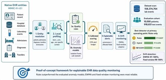
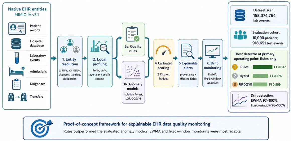
Entity-aware quality assessment may reduce false interpretations of electronic health record (EHR) data, but evidence from small, rule-aligned benchmarks cannot establish operational effectiveness. We revised H-StreamQ as a proof-of-concept framework and evaluated its laboratory component using the complete MIMIC-IV v3.1 labevents file (158,374,764 events; 313,442 patients). Ten thousand patients were sampled across laboratory-activity quintiles and split at patient level into training (6000), threshold-calibration (2000), and test (2000) groups. The independent test set contained 918,651 numeric laboratory events. Without excluding naturally alerted records, 54,788 mutually exclusive defects were introduced using subtle value shifts, unit/scale errors, mapping errors, delayed records, and patient-clustered correlated defects. Rules, a context-aware Isolation Forest, their union (Hybrid), a context-free Isolation Forest, Local Outlier Factor (LOF), and linear and radial-basis-function (RBF) One-Class support vector machines (OCSVMs) were compared at a threshold fixed by a 2.5% calibration alert budget. Patient-cluster bootstrap intervals and event-micro and patient-macro results were reported. Rules alone achieved the highest event-micro F1-score (0.637; 95% confidence interval [CI] 0.547–0.722), followed by Hybrid (0.576; 0.484–0.668) and RBF One-Class SVM (0.559; 0.433–0.670). Hybrid increased recall over rules by only 0.004 (95% CI 0.003–0.006) while reducing F1 by 0.061 and increasing the background-alert rate by 0.015. Context conditioning did not improve aggregate Isolation Forest performance. In six batch-level drift simulations, an exponentially weighted moving average (EWMA) and a fixed-window monitor detected 97–100% and 98–100% of changes, respectively, whereas a custom Hoeffding adaptive-window detector was more conservative and often missed smaller or recurrent changes. These results support H-StreamQ as an explainable research framework, not as a validated clinical or production system. Patient-macro F1, which weights every patient equally, was substantially lower than event-micro F1 for every method (rules 0.395 versus 0.637; Hybrid 0.320 versus 0.576), indicating that event-level performance is weighted towards high-activity patients. Precision and F1 are computed relative to injected synthetic labels and are not clinically adjudicated estimates. The entity-aware architecture spans patients, admissions, diagnoses, transfers, and dictionaries, but the quantitative detection benchmark evaluates the numeric laboratory component only; other entities are used for linkage and contextual attachment and are audited descriptively rather than evaluated against labels.

Graphical Abstract

1. Introduction

Electronic health records (EHRs) support clinical operations, quality reporting, research, and machine-learning development, but downstream conclusions depend on the reliability of source data. Digital-health datasets contain missing values, incompatible formats, duplication, delayed events, implausible measurements, and inconsistencies across related tables [1,2]. The consequences are not limited to model accuracy: quality defects can alter cohort definitions, bias subgroup estimates, and increase the burden of manual review.
Data quality is multidimensional and use-dependent. Classical work distinguishes completeness, consistency, accuracy, timeliness, and representational quality [3,4], while healthcare frameworks organize assessment around conformance, completeness, and plausibility [2]. The same value can have different interpretations across patients, encounters, laboratory items, and workflows. A missing numerical laboratory result can be legitimate when a categorical result is recorded; a value outside a reference interval can be clinically abnormal yet correctly represented; and a missing admission identifier can be valid for an outpatient event.
Operational tools already address important parts of this problem. The OHDSI Data Quality Dashboard (DQD) implements parameterized table-, field-, and concept-level checks for the Observational Medical Outcomes Partnership (OMOP) Common Data Model (CDM) and resolves approximately 4000 checks through the Kahn framework [5]. H-StreamQ is not proposed as a replacement for DQD or an OMOP validation tool. Its narrower contribution is to examine how linked native EHR entities, training-derived local boundaries, anomaly scores, explainable rules, and sequential quality-rate monitoring can be combined and evaluated without treating clinical abnormality as corruption.
Evaluating such a framework credibly imposes specific design requirements. A benchmark assembled only from the constraints a system already implements will overstate its performance; thresholds derived after removing records that existing alerts have flagged will yield optimistic estimates; and repeated corruptions of a small patient cohort do not constitute independent experimental units. This study therefore uses the full MIMIC-IV laboratory file for cohort construction, performs patient-disjoint training, calibration, and testing, retains naturally unusual records, introduces less rule-aligned and clustered defects, adds independent anomaly baselines, and quantifies uncertainty with patient-cluster bootstrap intervals rather than tests that assume independent observations.
The contribution is deliberately scoped as a rigorous proof-of-concept evaluation rather than evidence of real-world clinical effectiveness. The objectives are to: (i) formalize entity- and context-aware features and alert provenance; (ii) quantify performance on a substantially larger patient-level laboratory benchmark; (iii) compare deterministic rules, Isolation Forest variants, Local Outlier Factor (LOF), and One-Class support vector machine (OCSVM) methods; (iv) report patient-cluster uncertainty, event-micro and patient-macro results, error-specific recall, and subgroup alert-rate audits; and (v) evaluate sequential monitors under six drift mechanisms.
The study addresses five research questions. RQ1 asks how well training-derived rules and anomaly methods detect heterogeneous laboratory quality defects in a patient-disjoint test cohort. RQ2 asks whether adding a context-aware Isolation Forest to deterministic rules improves performance at a threshold fixed on an independent calibration cohort. RQ3 examines variation by error mechanism, event-micro versus patient-macro averaging, and patient-cluster uncertainty. RQ4 examines whether context conditioning or subgroup-calibrated thresholds consistently reduce background-alert-rate disparities. RQ5 compares adaptive, EWMA, and fixed-window monitors in terms of detection, delay, and false alarms across six simulated quality-drift mechanisms.
The remainder of the paper is organized as follows. Section 2 positions H-StreamQ relative to established data-quality and anomaly monitoring approaches. Section 3 describes the framework, linked entities, quality dimensions, and mathematical features. Section 4 presents the data, patient-level experimental design, comparators, statistical analysis, and drift simulations. Section 5 reports the empirical results. Section 6 discusses interpretation, operational governance, and limitations, and Section 7 concludes the paper.

2. Related Work

2.1. Data-Quality Frameworks for EHRs

General data-quality research established fitness for use as a multidimensional property [3,4,6,7,8]. The Data-Quality Modeling and Assessment Framework (DQMAF) automates profiling and quality-level classification on a general-purpose dataset [9]. Kahn et al. provide a harmonized healthcare terminology [2], the Machine-Learning Data-Quality Assurance framework (ML-DQA) operationalizes assurance for healthcare machine-learning pipelines [10], and the METRIC framework emphasizes fitness of medical data for a defined artificial-intelligence use case [11]. Complementary reviews and applied studies establish why these differences matter in practice: Declerck et al. synthesize frameworks, dimensions, and assessment methods for the secondary use of health data [12]; Reimer et al. develop an assessment framework for judging whether electronic medical record data are fit for research use [13]; and Dentler et al. show that data-quality defects propagate directly into computed hospital quality indicators [14]. These frameworks motivate systematic assessment but differ in data model, unit of analysis, and operational scope.
The OHDSI DQD is the strongest operational comparator for standardized observational data. It applies reusable check types across OMOP tables, fields, and concepts, reports transparent threshold evaluations, and has demonstrated value across real-world data networks [5]. Because the present data remain in native MIMIC-IV tables rather than an OMOP CDM instance, executing DQD on the same records would require an independently validated extract–transform–load (ETL) conversion and was outside the revised experiment. We therefore include DQD in positioning and capability comparison, but do not claim direct empirical superiority. DQMAF and ML-DQA were likewise considered as empirical comparators but could not be executed on the same records. DQMAF profiles static, general-purpose datasets and assigns quality levels at dataset rather than event granularity, so it emits no per-event decision that could be scored against the injected labels used here. ML-DQA specifies an assurance process, comprising provenance review, adjudication, and documentation steps carried out by a project team, rather than an executable detector, and therefore provides no artifact that can be applied to laboratory events. Both are retained in Table 1 as positioning references, and the comparative experiment instead benchmarks proposed rules against independent unsupervised detectors that do emit event-level scores.
Table 1 clarifies that H-StreamQ occupies a narrower position than the listed frameworks. Kahn et al. provide terminology rather than an executable detector; DQMAF focuses on general static profiling; ML-DQA and METRIC emphasize assurance and fitness for machine-learning use; and the OHDSI DQD provides mature checks for standardized OMOP data. H-StreamQ’s specific contribution is the combination of linked native-EHR semantics, locally derived event-level features, explicit alert provenance, comparative anomaly evaluation, and sequential monitoring. Its present limitations are equally important: it is not an OMOP validator, has not been prospectively deployed, and has not been validated with independently adjudicated natural errors.

2.2. Anomaly Detection, Context, and Representation

Isolation Forest isolates uncommon observations through short paths in randomized trees [17]. LOF compares local reachability density with neighboring observations [18], whereas OCSVM estimates a boundary around the support of predominantly normal data [19]. These methods detect different geometries and therefore provide meaningful independent baselines. In clinical data, however, a single global boundary can encode representation bias when normal distributions differ by age, sex, comorbidity, or care context. A context-conditioned boundary is a testable design choice, not an assumed improvement.
Missingness also requires caution. Under the Rubin framework, whether missing values can be ignored depends on the missingness mechanism [20]. H-StreamQ therefore does not delete records solely because a unit, admission identifier, or delay is missing. Missingness indicators remain features or review signals, and this study does not claim to distinguish missing completely at random (MCAR), missing at random (MAR), and missing not at random (MNAR) from the available tables.

2.3. Sequential Quality Monitoring

Healthcare workflows, device configurations, coding practices, and patient-mix change over time. Continuous monitoring is therefore necessary for maintaining clinical analytics [21]. Concept-drift research provides adaptive windows and sequential tests [22,23], while exponentially weighted moving average (EWMA) charts provide transparent sensitivity to sustained mean shifts [24]. The revised experiment distinguishes an original custom Hoeffding adaptive-window implementation from the official Adaptive Windowing (ADWIN) algorithm and compares it with EWMA and a fixed-window rate monitor under abrupt, gradual, recurrent, seasonal/autocorrelated, patient-mix, and multidimensional drift.

3. H-StreamQ Framework

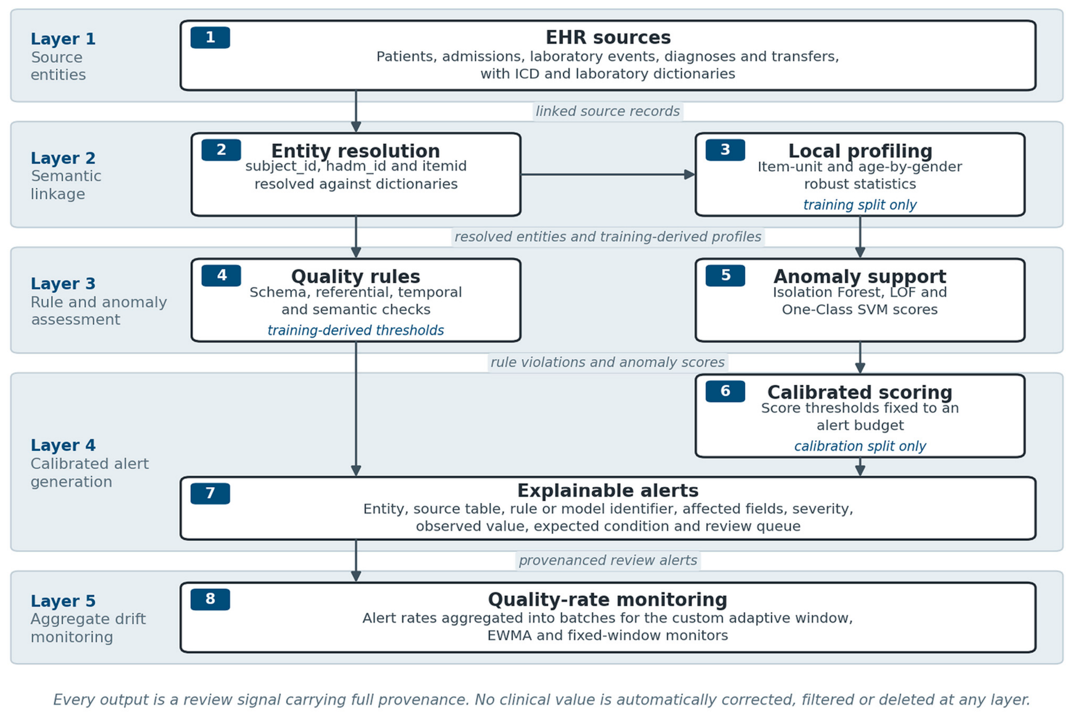
Figure 1 organizes the framework into five functional layers, namely source entities, semantic linkage, explainable rule and anomaly assessment, calibrated alert generation, and aggregate drift monitoring, within which eight numbered components carry distinct responsibilities. The figure shows component responsibilities and information flow rather than a deployment topology. It does not imply that a production interface with an electronic record system has been implemented, and no component automatically corrects, filters, or deletes a clinical value.

3.1. Entity-Aware Data Model

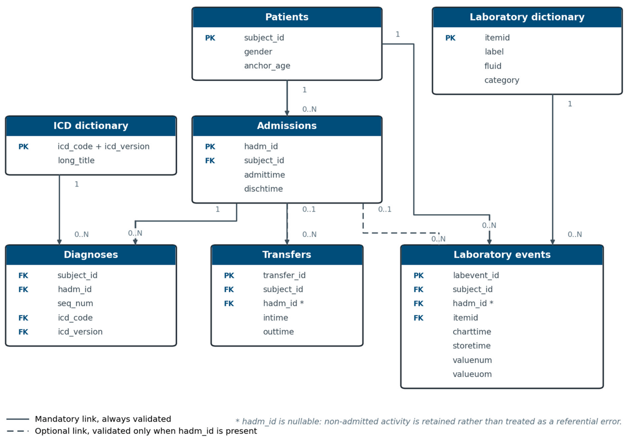
H-StreamQ treats subject_id as the longitudinal patient key and hadm_id as the admission key. Diagnoses, transfers, and laboratory events are linked to admissions when an admission identifier is available; ICD and laboratory dictionaries validate code and item semantics. Laboratory events without hadm_id are retained because MIMIC-IV includes non-admitted activity. This prevents a generic referential rule from converting contextually valid records into errors.
Figure 2 identifies which relationships are mandatory and which are contextual. Every laboratory item must be resolved to the laboratory dictionary, whereas an admission relationship is checked only when hadm_id is present. This distinction is central to entity awareness because the absence of an optional encounter link is not automatically classified as corruption.

3.2. Quality Dimensions and Explainable Alerts

Table 2 converts the framework’s quality concepts into operational checks. Completeness and referential checks depend on the applicable entity context; conformance and temporal checks compare observations with source semantics or training-derived profiles; and plausibility remains a review signal rather than a declaration that a clinically abnormal result is invalid.
Every alert carries the entity identifier, source table, rule or model identifier, affected fields, severity, observed value, expected condition, training/calibration provenance, and an explanation. Plausibility and subgroup findings are review signals. The framework neither overwrites clinical values nor filters records automatically.
Worked example. Consider a blood creatinine event with subject_id = 101, hadm_id = 5001, itemid = 50912, valuenum = 8.84, valueuom = ‘mg/dL’, charttime 10:00, and storetime 11:00. First, the entity layer verifies that subject 101 exists, admission 5001 belongs to that subject, and item 50912 resolves to creatinine. Second, schema and temporal rules verify a numeric payload, recognized unit, and non-negative one-hour delay. Third, the value is compared with training-only creatinine-by-unit statistics and, when sufficiently supported, the patient’s age-by-gender context; the example may therefore produce a high robust plausibility score without being called clinically erroneous. Fourth, the eight-feature vector is scored by the calibrated Isolation Forest. Fifth, rule and model evidence is combined with provenance into a review alert. Finally, alert counts are aggregated into time batches for EWMA, fixed-window, or custom adaptive monitoring. No value is automatically corrected or deleted at any step.

3.3. Mathematical Definition of Local Features and Isolation Forest

For a numeric result x from laboratory item j and unit u, training-only robust location and scale are defined by the median mju and interquartile range IQRju. When at least 100 training observations are available, the item-relative score is:
zju(x) = |x − mju|/(IQRju/1.349)
If IQR is zero, a non-zero training standard deviation is used; otherwise, the score is zero. A conditional score zjugc(x) is calculated analogously for age group g and gender c when at least 200 training observations support that context; otherwise, the item–unit score is used. Context is therefore a fallback hierarchy rather than a requirement that removes sparse groups.
The anomaly feature vector is x ∈ ℝ8: log(1 + zju), log(1 + zjugc), log(1 + non-negative storage delay), missing-unit indicator, unit-mismatch indicator, missing-delay indicator, negative-delay indicator, and an indicator that a context boundary was available. Median imputation is fitted within each model pipeline. For an Isolation Forest trained with subsample size n, the conventional normalized anomaly score is [17]:
s(x,n) = 2^(−E[h(x)]/c(n))
c(n) = 2H(n − 1) − 2(n − 1)/n
where E[h(x)] is the expected path length across trees and H is the harmonic number. Shorter expected paths produce larger anomaly scores. Implementation scores were oriented so that larger values indicated greater anomaly evidence.

4. Materials and Methods

4.1. Dataset, Full Scan, and Patient-Level Splits

The study uses MIMIC-IV v3.1 under credentialed PhysioNet access [25,26,27]. The complete labevents.csv.gz file was scanned with DuckDB 1.4.5 rather than loaded into memory. It contained 158,374,764 laboratory events from 313,442 patients, 447,689 admissions, and 976 laboratory item identifiers; 136,884,423 events had a numeric value. No alert-supported or clinically unusual record was excluded before cohort formation.
Patients with numeric laboratory events were ranked into five activity quintiles. Two thousand patients were sampled without replacement from each quintile with seed 2026. Within every quintile, patients were assigned 60%/20%/20% to training, threshold calibration, and testing. Consequently, no patient appeared in more than one split. Training-derived item, unit, context, delay, and rule profiles were never recomputed from calibration or test observations.
Table 3 separates the components that were empirically evaluated against labels from those implemented but audited descriptively, and from those that remain conceptual. Claims of measured detection performance in this study apply only to the first category.
Table 3. Implemented, audited, and conceptual components of H-StreamQ.
ComponentStatusEvidence in This Study
Numeric laboratory value, unit and delay checksImplemented and empirically evaluatedInjection benchmark; 918,651 test events (Section 5.2)
Context-conditioned anomaly scoring (age x gender)Implemented and empirically evaluatedSection 5.2, Section 5.3 and Section 5.4; Figure 3, Figure 4 and Figure 5
Anomaly baselines (IF, LOF, linear and RBF OCSVM)Implemented and empirically evaluatedSection 5.2
Batch-level drift monitoringImplemented; evaluated on simulated streamsSection 5.5; not validated on replayed EHR streams
Entity linkage across patients, admissions, diagnoses, transfers, dictionariesImplemented; descriptively auditedSection 5.1; review candidates, not labeled outcomes
Cross-entity temporal and referential rulesImplemented; descriptively auditedSection 3.1; no adjudicated labels available
Subgroup alert-rate auditImplemented; descriptive onlySection 5.4; not a validated fairness assessment
Streaming deployment, quarantine and governance workflowConceptualSection 6.6; no prospective implementation
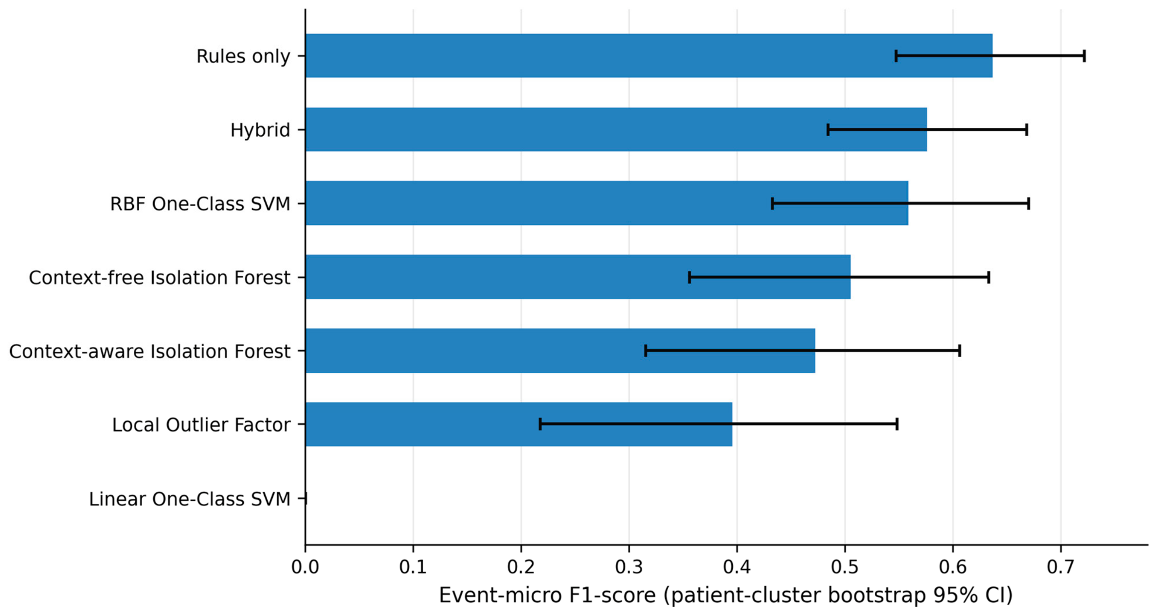
Figure 3. Event-micro F1-scores with patient-cluster bootstrap 95% confidence intervals. The deterministic rule baseline achieved the highest point estimate.
Information 17 00786 g003
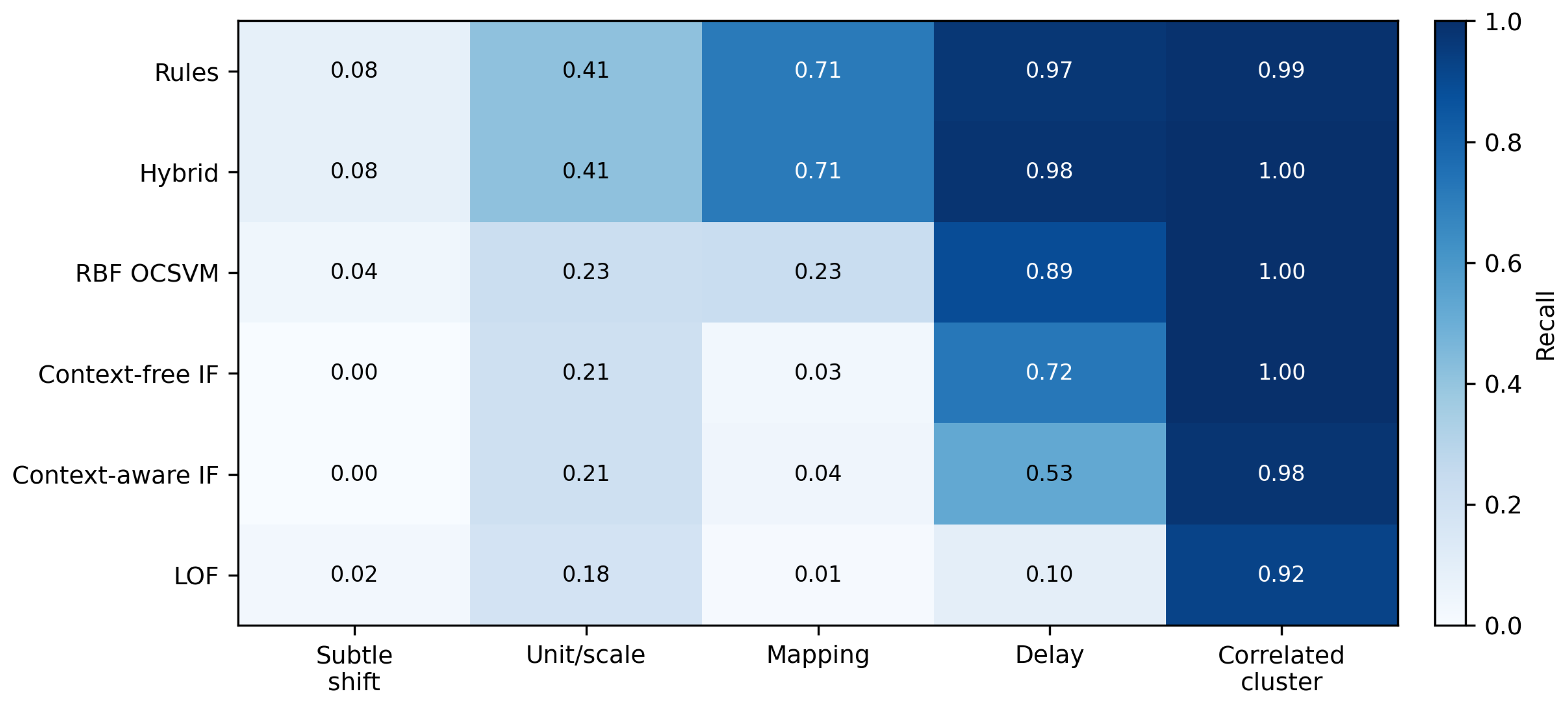
Figure 4. Recall by injected error mechanism at the primary operating point. No method was uniformly the strongest across mechanisms.
Information 17 00786 g004
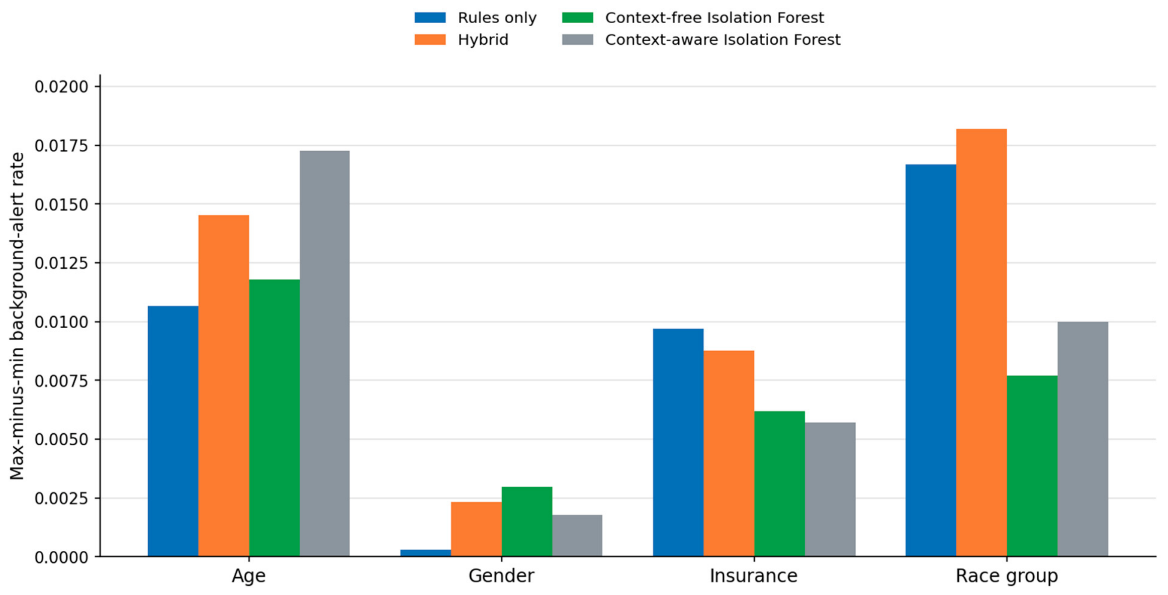
Figure 5. Maximum–minus–minimum background-alert rate across supported subgroups. Rates are descriptive because unmodified events were not clinically adjudicated.
Information 17 00786 g005
As Table 4 shows, the calibration and test cohorts are large enough to support independent operating-point selection and final evaluation, while patient-level separation prevents repeated measurements from the same patient from crossing splits. Similar median activity across splits reduces the chance that one group is dominated by unusually high-volume patients.
The complete patients (364,627 rows), admissions (546,028), diagnoses_icd (6,364,488), d_icd_diagnoses (112,107), transfers (2,413,581), and dictionary tables remained available for entity linkage and context attachment. The predictive benchmark focuses on numeric laboratory events because these tables supply the largest volume of directly comparable numeric observations for which item-, unit-, and context-level reference statistics can be derived entirely from training patients.

4.2. Leakage Control and Training-Derived Reference Statistics

Item–unit statistics were retained when at least 100 training events were available; 276 of 557 Item–unit groups met this criterion and covered 2,770,637 of 2,777,363 training events (99.76%). Age-group-by-gender context statistics required at least 200 events; 849 of 3488 context groups met this criterion and covered 2,703,827 training events (97.35%). The most frequent non-missing training unit defined the canonical unit per item. Test data retained 300,962 clinically flagged events and 301,525 values outside supplied reference intervals; these were not treated automatically as quality errors.

4.3. Realistic Mixed-Error Benchmark

The unchanged test cohort served as the benchmark substrate. Five mutually exclusive mechanisms were assigned deterministically. Event-level shifts and scale errors were combined with patient-day bursts and patient-cluster defects to avoid uniform independent corruption. Mechanisms are mutually exclusive at the label level so that recall can be attributed unambiguously to a single defect type. Defects nevertheless compound within records: the correlated-cluster mechanism applies both a value shift and an extended storage delay to the same events, and both burst mechanisms concentrate multiple defective events within a patient-day. Coding changes, such as a mid-stream revision of an item dictionary or an ICD version transition, were not simulated, because MIMIC-IV supplies a single consolidated dictionary release and a credible coding-change benchmark would require versioned dictionaries that the source does not expose; this remains a limitation. The resulting 54,788 injected events represented 5.964% of the test set. Records assigned ‘none’ were unmodified but could still contain naturally occurring quality concerns; therefore, alerts on this group are described as background alerts rather than clinically adjudicated false positives.
Unit/scale factors were prespecified for creatinine, urea nitrogen, glucose, total calcium, magnesium, and phosphate. Mapping pairs were sodium/chloride and hematocrit/RDW, chosen because they share observed units while representing different concepts. Feature-effect validation confirmed that median robust scores increased from 0.674 to 2.481 for subtle shifts, 0.639 to 3.628 for unit/scale errors, and 0.674 to 7.824 for mapping errors; median log delay increased from 0.750 to 3.808 for delayed records and from 0.773 to 4.147 for correlated clusters.
Table 5 shows that no single transformation dominates the benchmark and that 94.0% of events remain unmodified. The clustered mechanisms deliberately concentrate some defects within patients or patient-days, while the subtle-shift and stale-unit transformations are not reducible to simple identifier-validity checks.

4.4. Compared Methods and Threshold Calibration

Rules used reference profiles learned only from training data. The executed value rule used a fixed conditional robust-score threshold of 4.72. Under Equation (1), this is the standardized equivalent of a two-sided 3.5-interquartile-range boundary (3.5 × 1.349 = 4.7215). The value was adopted a priori as a fixed rule configuration and was not estimated from calibration or test labels. Item-specific storage-delay thresholds used the 99.5th training percentilewhen at least 500 valid delays were available and otherwise used the global 99.5th percentile (23.067 h). Unit presence and canonical-unit rules required a training share of at least 0.99. Hybrid was the logical union of rules and context-aware Isolation Forest alerts.
All anomaly thresholds were fixed using the independent calibration cohort at alert budgets of 1%, 2.5%, and 5%; the 2.5% budget was designated as the primary operating point before evaluating test labels. This thresholding design separates training, operating-point calibration, and testing at patient level.
Table 6 distinguishes operational rules, the two Isolation Forest variants, and three external anomaly baselines. LOF tests local-density departures, OCSVM tests support-boundary methods, and the context-free Isolation Forest isolates the contribution of conditional features. These implementations permit algorithmic comparison even though a direct execution of OHDSI DQD on native MIMIC-IV tables is not methodologically valid without an independently verified OMOP transformation.

4.5. Evaluation and Cluster-Aware Statistical Analysis

Injected events defined positives for benchmark evaluation. Precision, recall, F1, alert rate, receiver-operating-characteristic area under the curve (ROC-AUC), and average precision (AP) were calculated. Because unmodified events were not clinically adjudicated, the proportion alerted among them is termed the background-alert rate (BAR). The primary binary metrics are:
Precision = TP/(TP + FP); Recall = TP/(TP + FN)
F1 = 2 × Precision × Recall/(Precision + Recall)
Patients, rather than repeated corruption runs, were the resampling unit, because repeated corruptions of the same cohort are not independent experimental units. Two thousand patient-cluster bootstrap repetitions produced 95% percentile confidence intervals for model metrics and for paired model differences; no hypothesis test assuming independent observations was applied. Two contrasts were designated primary before test labels were examined: rules versus Hybrid, and context-aware versus context-free Isolation Forest. All remaining pairwise contrasts are exploratory and are reported without multiplicity adjustment. Because marginal intervals for different methods are computed on the same patients, overlap between them does not imply that the corresponding paired difference includes zero; paired difference intervals are therefore reported for the contrasts of interest. Event-micro metrics pool event-level confusion counts; patient-macro metrics first calculate each patient’s metric and then average supported patient estimates. Recall was also reported by error mechanism.
A representation audit measured background-alert rates across age, gender, race group, and insurance categories with at least 1000 events, excluding UNKNOWN from disparity ranges. These rates are not fairness-adjusted error rates because unmodified events lack independent clinical adjudication. An exploratory age-by-gender calibration used subgroup thresholds only when a calibration subgroup contained at least 10,000 events; otherwise, the global threshold was retained.

4.6. Drift Simulation and Mathematical Definitions

Six event streams of length 5000 were simulated: abrupt, gradual, recurrent, seasonal/autocorrelated, patient-mix, and multidimensional deterioration. Event indicators were aggregated into 50 consecutive batches of 100 events. Ten pre-change batches estimated baseline mean and standard deviation. Each scenario–detector–parameter combination was repeated 100 times with seeds 2026–2125.
For batch-rate Yt, EWMA was updated as [24]:
Zt = λYt + (1 − λ)Zt−1
UCL = μ0 + Lσ0 √[λ/(2 − λ)]
with L = 3 and λ in {0.05, 0.10, 0.20}. The fixed monitor compared the mean of w recent batches with μ0 + 3σ0/√w, for w in {5, 10, 15}. The custom detector compared candidate left and right subwindows using:
ε = √[0.5 ln(4/δ)(1/nl + 1/nR)]
and signaled when the absolute mean difference exceeded ε. This is an original Hoeffding-bound adaptive-window detector rather than the reference ADWIN implementation [23]; it has not been cross-validated against that reference and is reported under the custom name throughout. Values δ ∈ {0.01, 0.05, 0.10} were evaluated. Detection and false-alarm proportions use Wilson 95% intervals; detection delay is reported as a median with the empirical central 95% range among detected runs. Hoeffding’s inequality requires bounded random variables, and the constant 0.5 in Equation (8) is the variance proxy appropriate to variables supported on the unit interval. The detector therefore operates on normalized batch quality rates rather than on raw counts or unbounded continuous values. Each batch contributes the proportion of flagged events among its 100 observations, which lies in [0, 1] by definition; this proportion is divided by a prespecified operational rate limit of 0.15 and clipped to [0, 1], so the quantity entering Equation (8) is a normalized quality rate on the unit interval. The comparison in Equation (8) is between the arithmetic means of the left and right subwindows of these normalized rates, and the boundedness condition is therefore satisfied by construction rather than by assumption. The operational rate limit is a monitoring configuration parameter representing the alert rate at which a batch would be escalated regardless of statistical evidence; normalizing against it makes detector sensitivity interpretable relative to that operational ceiling.
Events were aggregated into batches of 100 because a batch quality rate must be estimable with acceptable variance before it can be monitored: at a baseline error rate of 0.02, a 100-event batch yields a binomial standard error of approximately 0.014, which is small relative to the smallest simulated post-change shift, whereas smaller batches produce rate estimates too noisy to separate drift from sampling variation. Each 5000-event stream therefore yields 50 batch observations. Ten pre-change batches, corresponding to 1000 events, estimated the baseline mean and standard deviation; this is sufficient to estimate a proportion near 0.02 with a standard error of roughly 0.004 while leaving the majority of the pre-change period available for false-alarm assessment, and the detectors additionally apply a warm-up period during which no alarm may be raised, so baseline estimation cannot itself trigger a detection.
Drift onset was defined at event position 2000, corresponding to batch 20, for the abrupt, gradual, seasonal/autocorrelated, patient-mix, and multidimensional scenarios. The recurrent scenario was the prespecified exception: its first elevated-rate phase began at event position 1500, corresponding to batch 15; the stream returned to baseline from events 2500 to 3499 and entered a second elevated-rate phase at event position 3500. For abrupt drift, onset is the step change; for gradual drift, it is the first event at which the error probability begins to increase, with the ramp completing 750 events later; for seasonal/autocorrelated drift, it is the onset of the elevated oscillation; and for multidimensional drift, it is the first event at which any monitored quality dimension begins to deteriorate. Detection delay is measured in batches from the scenario-specific onset batch to the first alarm at or after onset. Alarms raised before the applicable onset batch are recorded as pre-change false alarms rather than detections, and such runs contribute no delay. Runs producing no alarm at or after onset are recorded as missed and assigned a missing delay; missed and false-alarm runs are excluded from delay summaries, so reported medians and ranges describe detected runs only. Each detector was evaluated to first alarm within a run, with no post-detection cooldown or re-arming, so repeated alarms within a run do not affect the reported statistics. For the recurrent scenario, delay is measured relative to the first elevated phase at batch 15 only; alarms raised during later phases are not credited as additional detections, and a run is recorded as detected if any alarm occurs at or after that first onset batch. The recurrent scenario in the run-level file provided in the Supplementary Materials was calculated using batch 15 as the onset and therefore requires no recalculation.

4.7. Software and Reproducibility

The revised analysis used Python 3.9.13, NumPy 1.21.5, pandas 1.4.4, scikit-learn 1.0.2, SciPy 1.9.1, DuckDB 1.4.5, and PyArrow 21.0.0 on macOS. Seed 2026 governed cohort sampling, benchmark transformation, model fitting, and patient-cluster bootstrap resampling; the drift sensitivity experiment used seeds 2026–2125 across 100 repetitions. The notebook provided in the Supplementary Materials contains 43 executed cells with no stored errors, and aggregate CSV, Parquet, and figure outputs accompany the revision. Restricted MIMIC-IV records are not redistributed.

5. Results

5.1. Cohort Scale, Coverage, and Retained Natural Variation

Among 310,313 patients with numeric laboratory results, the mean number of events was 441.1, the median was 129, the 90th percentile was 1047, and the maximum was 40,154. The selected 10,000-patient cohort contained 4,571,914 numeric events. Patient activity was similar across splits: medians were 130, 131, and 134 events in training, calibration, and testing. In the test set, item-level robust scores were available for 916,383 of 918,651 events and context-level scores were used for 880,428 events.
Natural variation was deliberately retained. The test cohort included 82,078 missing units, 276 missing storage times, 300,962 clinical flags, and 301,525 values outside supplied reference intervals. These counts describe source characteristics rather than confirmed errors. Patients, admissions, diagnoses, transfers, and dictionary tables were used for entity linkage and contextual validation, but no unadjudicated cross-entity finding was used as a benchmark label.

5.2. Primary Model Comparison

Table 7 reports precision, recall, F1 with patient-cluster bootstrap intervals, background-alert rate, ROC-AUC, and average precision for all seven compared methods at the primary operating point.
Figure 3 shows that rules alone achieved the highest F1 point estimate, and that marginal intervals overlap substantially even where the corresponding paired differences exclude zero. Hybrid increased recall by 0.0044 relative to rules (95% CI 0.0027–0.0065), but precision decreased by 0.0983, F1 decreased by 0.0605 (95% CI −0.0666 to −0.0523), and BAR increased by 0.0152. Context-aware Isolation Forest also underperformed the context-free Isolation Forest by 0.0332 F1 (95% CI −0.0432 to −0.0249) and RBF OCSVM by 0.0863 (95% CI −0.1178 to −0.0621). For the linear One-Class SVM, the executed notebook defined anomaly evidence as the negative of scikit-learn’s score_samples output, consistent with the library convention that larger raw values indicate greater inlier support, so the reported ROC-AUC of 0.149 is not an uncorrected sign inversion. A value below 0.5 nevertheless indicates systematically inverted ranking rather than uninformative scoring, and the geometry of a linear one-class boundary explains why: the boundary separates the training data from the origin, so events with uniformly large feature magnitudes, namely the high robust scores and long logarithmic delays that characterize the injected defects, lie farther from the origin and receive greater inlier support. Reversing the ranking yields 0.851, confirming that the model orders events informatively but in the wrong direction. A linear support boundary is therefore unsuitable for this feature geometry, and the model is retained as an interpretable negative baseline. Thus, RQ2 is answered negatively at the prespecified primary operating point: the hybrid and context conditioning did not improve aggregate F1. Because unmodified records were not independently adjudicated, the reported precision is a synthetic-label precision rather than a clinical estimate. A method that correctly identifies genuine, naturally occurring defects among the nominally unmodified records is penalized by this benchmark as though those alerts were errors. The value 0.590 for rules should therefore be read as precision with respect to injected labels under a benchmark that treats all other alerts as background, and not as an estimate of the proportion of clinically valid alerts. The compared methods do not operate at matched alert burden. Rules produced a total test alert rate of 0.0699 against 0.0498 for the context-aware Isolation Forest, 0.0512 for the context-free variant, and 0.0570 for the RBF One-Class SVM, so rules issue approximately 1.4 times as many alerts as the context-aware model, and part of the rules’ advantage could in principle reflect this larger alert budget rather than better discrimination. The operating-point sensitivity analysis addresses this directly. Raising the calibration alert budget from 2.5% to 5% approximately doubles each anomaly detector’s alert rate, placing all of them above the rules’ 0.0699, yet event-micro F1 does not rise: it falls to 0.439 for the context-aware Isolation Forest, 0.472 for the context-free variant, 0.495 for the RBF One-Class SVM, and 0.359 for LOF. No anomaly detector approaches the rules’ 0.637 at any evaluated budget, including budgets granting a larger alert burden than the rules themselves consume, so the conclusion is not an artifact of operating-point selection. Hybrid is a separate case: as the union of rules and the context-aware Isolation Forest it cannot produce a lower alert rate than rules alone, and its 0.0845 alert rate and 0.046 background-alert rate are structural consequences of the union rather than a tunable operating point.
Table 8 reports interval estimates for every metric, and Table 9 reports the paired contrasts underlying the comparisons above. Both prespecified contrasts exclude zero for F1. The background-alert-rate difference between the two Isolation Forest variants and the precision difference between the RBF One-Class SVM and rules both include zero, so neither is distinguishable at this sample size.
Operating-point sensitivity was examined using calibration alert budgets of 1%, 2.5%, and 5%. Context-aware Isolation Forest F1 was 0.430, 0.472, and 0.439 across these budgets; context-free Isolation Forest F1 was 0.506, 0.505, and 0.472; RBF OCSVM F1 was 0.580, 0.559, and 0.495; and LOF F1 was 0.375, 0.396, and 0.359. Thus, the precision–recall balance changed with the alert budget, but no tested threshold made the context-aware Isolation Forest the strongest method.
A separate targeted hyperparameter sensitivity analysis completed 16 configurations: eight context-aware Isolation Forest combinations of max_samples in {256, 1024, 4096, 16,384} and n_estimators in {100, 300}; five LOF settings with n_neighbors in {10, 20, 35, 50, 100}; and three RBF OCSVM settings with nu fixed at 0.01 and gamma in {scale, auto, 0.1}. Across these configurations, F1 ranged from 0.2491 to 0.4911 for context-aware Isolation Forest, from 0.2514 to 0.4165 for LOF, and from 0.4692 to 0.4989 for RBF OCSVM. The best configuration within each targeted grid was max_samples = 16,384 with 300 trees for context-aware Isolation Forest (F1 = 0.4911), n_neighbors = 100 for LOF (F1 = 0.4165), and gamma = 0.1 with nu = 0.01 for RBF OCSVM (F1 = 0.4989). None exceeded the rules-only F1 of 0.637. These 16 completed configurations provide a targeted robustness check, not exhaustive hyperparameter optimization; they do not establish invariance across the full parameter space. Full configuration-level results are supplied in hyperparameter_sensitivity_partial.csv.

5.3. Error-Specific, Event-Micro, and Patient-Macro Results

As Figure 4 shows, rules detected mapping errors (recall 0.711), delays (0.972), and correlated clusters (0.991), but detected only 0.083 of subtle shifts and 0.411 of unit/scale errors. RBF OCSVM improved anomaly-only coverage of subtle shifts (0.035 versus 0.002 for both Isolation Forest variants) and mapping errors (0.233), while detecting 0.890 of delays and all correlated clusters. Context-aware Isolation Forest detected 0.527 of delays and 0.977 of correlated clusters but very few subtle or mapping errors. These results show that the benchmark is not trivially aligned with any single detector.
As Table 10 shows, patient-macro F1 was lower than event-micro F1 for every method, indicating that aggregate event counts emphasize high-volume patients. This gap supports reporting both views and limits claims of uniform patient-level reliability. The gap is large for every method and is not a minor sensitivity finding. Two features of the design contribute. First, laboratory activity is highly skewed: the median patient contributes 129 numeric events while the maximum contributes 40,154, so event-level averages are necessarily weighted towards a minority of patients. Second, the cohort was sampled across activity quintiles rather than by simple random sampling, which deliberately over-represents low-activity patients relative to the natural MIMIC-IV population. The estimand evaluated here is therefore performance on an activity-stratified cohort rather than performance on the source population; a simple random sample would contain proportionally more low-activity patients and would likely widen the micro-macro gap further. The patient-macro column should be treated as the more conservative estimate of per-patient reliability.

5.4. Subgroup Alert-Rate Audit

Figure 5 shows that the context-aware Isolation Forest did not uniformly reduce subgroup disparity. Relative to context-free Isolation Forest, its age-group disparity was larger (0.0173 versus 0.0118) and race-group disparity was larger (0.0100 versus 0.0077), while gender disparity was smaller (0.0018 versus 0.0030) and insurance disparity was slightly smaller (0.0057 versus 0.0062). Age-by-gender threshold calibration reduced supported age-group background rates to 0.0242–0.0271, but aggregate F1 remained essentially unchanged (0.471 versus 0.472). The result supports monitoring and calibration, not a claim of fairness.

5.5. Drift Detection and Sensitivity

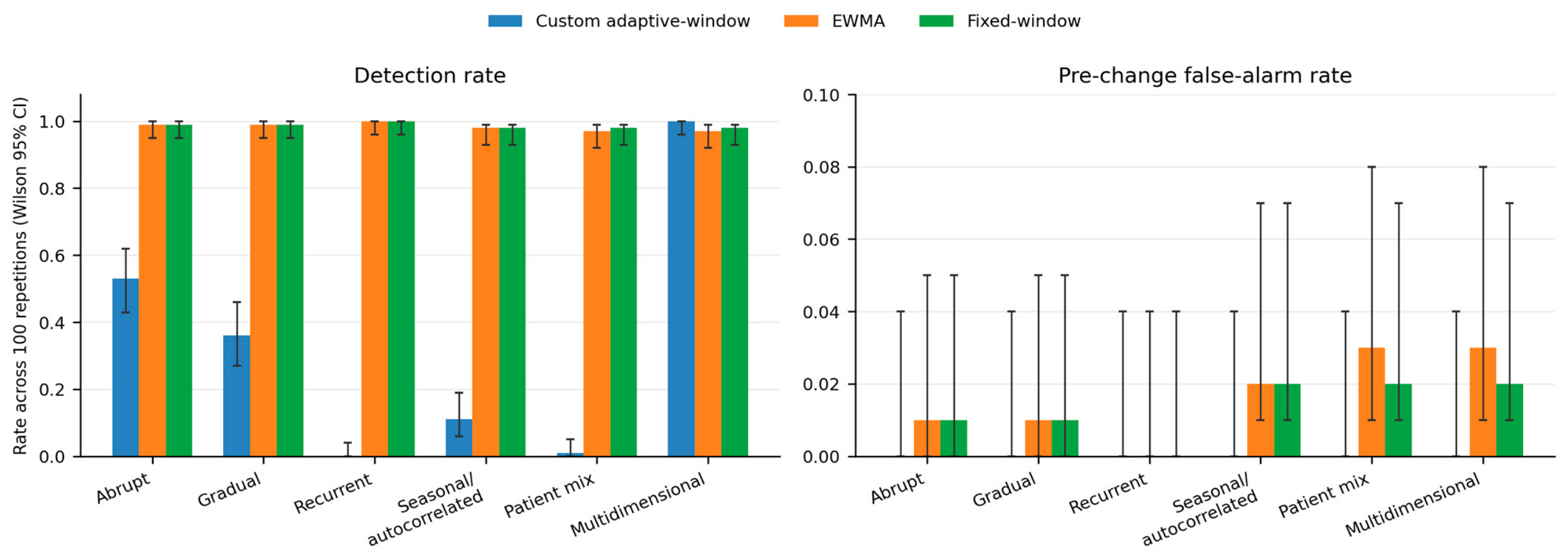
Figure 6 summarizes detection and pre-change false-alarm rates across the six scenarios with Wilson 95% intervals, and Table 11 reports the corresponding representative parameter settings. Table entries are detection rate/false-alarm rate (FAR)/median delay in 100-event batches, with Wilson 95% intervals for the two proportions. EWMA and the fixed monitor detected 97–100% and 98–100% of changes, respectively, with false-alarm rates no greater than 0.03 and median delays of 2–8 batches. The custom detector generated no pre-change alarms but missed recurrent drift and nearly all patient-mix and seasonal/autocorrelated changes. Sensitivity analysis across all nine parameter settings, comprising 5400 simulation runs, is provided in the Supplementary Materials file drift_analysis/drift_parameter_sensitivity.csv, with the full run-level output in drift_analysis/drift_simulation_results_5400_runs.csv. RQ5 therefore favors EWMA or a transparent fixed-window policy for these simulations; the custom detector is reported as an original, externally unvalidated implementation.

6. Discussion

6.1. Principal Findings

The framework remains useful for expressing healthcare semantics, training-derived boundaries, alert provenance, and multi-level monitoring, but the benchmark does not support claims of near-perfect effectiveness. Rules were the strongest primary baseline, Hybrid gained very little recall at a meaningful cost in precision and background alerts, and the context-aware Isolation Forest did not outperform its context-free comparator or RBF OCSVM.
This negative result is informative. Deterministic data-quality constraints directly encode unit, mapping, and latency expectations and remain difficult for generic unsupervised models to replace. Conversely, subtle shifts and unit conversions remained challenging for rules and all anomaly models, showing why a benchmark designed only from implemented constraints can exaggerate performance. Different methods were strongest for different mechanisms, supporting an ensemble only when its alert policy is calibrated to operational costs rather than assumed to improve F1.

6.2. What Entity and Context Awareness Currently Demonstrate

Entity awareness remains valuable for defining when a rule applies and for explaining alerts: item–unit profiles, optional admission links, dictionary resolution, and event-time relationships prevent obvious semantic misclassification. Statistical context awareness produced a more nuanced result. Age-by-gender conditioning did not improve aggregate Isolation Forest performance and had mixed effects on subgroup background rates. Therefore, context should be treated as a hypothesis to validate locally, not a guaranteed fairness or accuracy improvement.
The eight-dimensional feature space mixes four binary indicators with log-transformed continuous scores, and this heterogeneity offers a plausible geometric explanation for the observed degradation. An Isolation Forest isolates a point by recursively selecting a dimension uniformly at random and a split value uniformly between the observed minimum and maximum of that dimension. A binary indicator admits only one informative split point, so whenever such a dimension is selected, the minority class is separated at an expected depth close to one. Indicator dimensions therefore contribute very short path lengths to the expected path length whenever the indicator is rare, irrespective of whether the record carries an injected defect. Log-transformed continuous scores behave differently: isolating a tail observation requires several successive splits, and it is these dimensions that carry the discriminative signal for subtle value shifts and unit errors.
Because the expected path length averages over dimensions drawn uniformly at random, the informative continuous dimensions compete for selection with indicators whose depth contribution is largely independent of defect status. Adding the conditional context score increases the dimensionality of this competition without proportionally increasing discriminative information, because 2.65% of test events fall outside a supported age-by-gender context and receive a fallback value. The additional dimension is therefore partly redundant with the item–unit score and partly degenerate, which dilutes rather than sharpens the expected path length. We offer this as a mechanistic hypothesis consistent with the observed 0.0332 F1 deficit of the context-aware variant relative to its context-free counterpart, not as a proven account; establishing it would require ablating individual feature dimensions and measuring the change in expected path length directly, which we identify as future work. It nevertheless suggests that context should be introduced through separate conditional models or through score-level combination rather than by extending a single isolation feature vector.

6.3. Relationship to OHDSI DQD and Existing Methods

H-StreamQ is complementary to OHDSI DQD. DQD provides a mature, systematic, and configurable assessment layer for OMOP CDM instances [5]. H-StreamQ operates on linked native EHR entities and explores event-level anomaly signals and quality-rate drift. A fair head-to-head comparison requires the same data represented in a validated common model and a preregistered, independently adjudicated error corpus. The present study therefore compares anomaly algorithms directly but limits DQD to capability positioning.

6.4. Representation, Missingness, and Operational Accommodation

The subgroup audit shows why global or conditional thresholds should not automatically filter records. Background-alert-rate differences persisted across age, race, and insurance groups, and threshold calibration equalized selected rates without improving overall F1. Similarly, missing units, delayed encounters, and irregular care patterns may be informative and potentially MNAR [20]. H-StreamQ should route such findings with provenance and subgroup context, support threshold review and audit, and avoid deleting records or declaring clinical invalidity without adjudication. Equalized false-positive-rate constraints cannot be claimed until true labels are independently established within each subgroup.
Interpreting subgroup alert-rate differences requires distinguishing two things that a rate comparison alone cannot separate. A statistical disparity exists whenever background-alert rates differ across groups. A discriminatory boundary exists only when a threshold flags biologically normal variation associated with age, sex, or ancestry as an anomaly, for example, when a model fitted predominantly on a majority population rejects reference values specific to a minority group as outliers. These are not the same finding. If an elevated alert rate in an older or a particular race group reflects genuine physiological deviation arising from differences in disease prevalence, comorbidity burden, or care intensity, then the threshold produces a statistical difference without being discriminatory. Conversely, a numerically equal alert rate across groups is no guarantee that the boundary is fair, since equality can be achieved by suppressing genuine signal in one group.
Our evaluation cannot distinguish these cases. The unmodified events on which background-alert rates are computed have not been clinically adjudicated, so the cause of any observed disparity, whether genuine physiological deviation, genuine data-quality defect, or inappropriate boundary placement, is not identifiable from the available labels. This has a direct consequence for fairness constraints. Enforcing an equalized false-positive-rate constraint without ground-truth labels would force the boundary in the higher-rate group outward until its measured rate matched the reference group. If the elevated rate reflected genuine pathological abnormality rather than an inappropriate threshold, this would systematically suppress true clinical signal in exactly the group whose data is already least well represented, misclassifying pathological abnormalities in minority groups as normal and potentially delaying necessary medical intervention. The apparent fairness gain would be purchased with a concrete clinical harm that the metric itself cannot detect. We therefore report subgroup alert rates as descriptive monitoring outputs and explicitly decline to impose an equalized-rate constraint; establishing whether any observed disparity constitutes a discriminatory boundary requires adjudicated labels stratified by subgroup, which we identify as a prerequisite for any fairness claim rather than as an optional refinement.

6.5. Drift Monitoring Implications

The drift experiment does not support treating a conservative adaptive window as generally reliable. Under smaller and more varied changes, the custom Hoeffding detector avoided false alarms but often missed drift. EWMA and the fixed monitor were substantially more sensitive with a small false-alarm cost. This supports a transparent tiered policy: use EWMA or fixed windows for early warning, require confirmation or domain review before intervention, and retain the custom detector only as a conservative secondary signal unless independently validated against official ADWIN. This recommendation is limited to the simulated batch-rate settings evaluated here and does not extend to replayed EHR event streams, whose autocorrelation and non-stationarity may differ substantially from the simulated processes.

6.6. Integration into Hospital Data Governance

A hospital deployment should begin in silent-monitoring mode rather than by automatically rejecting records. H-StreamQ alerts would enter an existing data-quality dashboard or ticketing queue with the source entity, affected field, rule/model provenance, severity, and supporting context. Data stewards could triage structural and referential defects; laboratory informatics teams could assess units, mappings, and device-related changes; and clinical domain owners could adjudicate plausibility signals. Only locally approved deterministic failures should be eligible for staging quarantine, while anomaly and subgroup signals should remain review-only until prospective validation establishes action thresholds.
A specific risk arises when quality signals are used upstream of secondary data use rather than only at the point of care. If clinical data from a minority group are flagged as quality errors at an unjustifiably high rate, and if flagged records are then filtered from the construction of machine-learning training sets or clinical study cohorts, the exclusion compounds. Models trained on the surviving records become progressively better fitted to the majority population, their residuals on the under-represented group grow, and any subsequent quality model calibrated on those residuals flags the same group more often still. The result is a self-reinforcing cycle in which a data-quality tool intended to improve reliability instead narrows the population that downstream evidence describes, undermining health equity through an accumulation of individually defensible filtering decisions. This risk is the principal reason the framework is specified as review-generating rather than record-filtering, and it is why subgroup alert rates should be audited routinely rather than only at deployment.
Reasonable accommodation in this setting means declining to discard data on the basis of a uniform algorithmic threshold, and designing instead for human adjudication. Two design commitments follow. First, an alert should never impose a hard stop on a clinical order or medication workflow; it should present as a soft warning requiring acknowledgement, so that a clinician retains the ability to proceed with a value that is unusual for the reference population but correct for the patient in front of them. Second, the alert should carry the contextual information needed to make that judgment rather than a bare anomaly flag: the locally applicable reference range for the patient’s age, sex, and where clinically appropriate ancestry, alongside the observed value, the expected condition, and the provenance of the rule or model that generated the signal. Displaying the local distribution rather than a single global boundary converts the alert from an assertion that the value is wrong into evidence the clinician can weigh, which is the only form in which a quality signal can be safely surfaced in a population whose normal ranges the training data may not fully represent.
Governance would require a versioned registry of rules, training cohorts, thresholds, model artifacts, owners, approvals, and rollback criteria; routine subgroup and alert-volume audits; and escalation paths from data stewards to clinical safety, privacy, and information-technology governance. Technical barriers include heterogeneous identifiers and units, EHR-vendor interfaces, transformation lineage, delayed or replayed messages, compute and latency constraints, and restricted access to patient context. Organizational barriers include unclear data ownership, limited adjudication capacity, alert fatigue, competing definitions of fitness for use, change-management burden, and the need to demonstrate benefit without worsening subgroup exclusion. A staged pathway—silent observation, retrospective adjudication, prospective shadow validation, and only then controlled intervention—is therefore more appropriate than immediate production filtering.

6.7. Limitations

First, the larger evaluation uses one institution’s MIMIC-IV laboratory data and synthetic benchmark labels. It does not establish external, temporal, or production validity. Second, naturally occurring quality problems in unmodified events were not independently adjudicated; consequently, background-alert rate is not a definitive clinical false-positive rate. Third, although the complete laboratory file was scanned, the model benchmark uses a stratified 10,000-patient cohort and computationally bounded training samples for LOF, OCSVM, and Isolation Forest.
Fourth, the five mechanisms are more realistic than uniform rule-matched injections but cannot reproduce every coding change, device malfunction, mapping failure, or MNAR process. Fifth, subgroup analyses are descriptive and race/insurance information is unavailable for many events without linked admissions. Sixth, the custom adaptive-window implementation is not official ADWIN, and all drift results remain Monte Carlo simulations of batch quality rates rather than replayed EHR streams. Seventh, although the fixed 4.72 value boundary is mathematically equivalent to 3.5 interquartile ranges, it was adopted as a design constant rather than derived from a cohort-specific quantile, and all rule thresholds require prospective prespecification and independent validation. Eighth, the benchmark reflects a single corruption realization under one seed, so the reported intervals capture variation across patients but not across alternative assignments of the injected defects; a multi-seed replication was identified as valuable during review but could not be completed within the revision window because it requires re-executing the full benchmark and evaluation pipeline against the credentialed extract, and is accordingly listed as the first priority for a subsequent study. Ninth, the completed hyperparameter analysis was a targeted 16-configuration grid rather than exhaustive optimization. It varied forest size and subsample size for the context-aware Isolation Forest, neighborhood size for LOF, and kernel scale for the RBF OCSVM with nu fixed at 0.01. It did not sweep the context-free Isolation Forest, linear OCSVM, alternative RBF OCSVM nu values, feature sets, or interactions across the full parameter space. The finding that none of the 16 tested configurations outperformed rules therefore strengthens the result only within this targeted grid; the conclusion that context conditioning did not improve aggregate Isolation Forest performance remains limited to the primary configurations directly compared.
Finally, the study evaluates detection, not automatic correction, throughput, alert actionability, or clinical benefit. Future work should include independently adjudicated natural cases, external and temporal validation, OMOP conversion for direct DQD comparison, hierarchical patient/admission modeling, prospective stream replay, and stakeholder assessment of alert costs.


7. Conclusions

This study demonstrates an explainable research framework for linked EHR quality assessment, but it does not validate a production system. A patient-disjoint benchmark of 918,651 laboratory events showed that deterministic rules using training-derived reference profiles outperformed the proposed Hybrid and the evaluated anomaly detector configurations at the prespecified operating point. The Hybrid’s small recall gain did not compensate for lower precision, lower F1, and more background alerts, and context conditioning did not improve aggregate Isolation Forest performance. These findings give a realistic account of the framework’s strengths and failure modes rather than a claim of near-perfect detection. Two qualifications bound these conclusions. Precision and F1 are computed relative to injected synthetic labels; because unmodified records were not clinically adjudicated, they are benchmark quantities rather than estimates of clinically valid alert proportions, and a method detecting genuine natural defects among unmodified records is penalized by this design. Patient-macro F1 was also substantially lower than event-micro F1 for every method (rules 0.395 versus 0.637), so per-patient reliability is weaker than event-level aggregates suggest.
Entity semantics, patient-level separation, calibrated thresholds, cluster-aware uncertainty, error-specific reporting, subgroup audits, and varied drift scenarios materially strengthen the evidence. EWMA and fixed-window monitoring were the most reliable simulated drift detectors, while the custom Hoeffding detector was conservative and insensitive to several changes. H-StreamQ should therefore be regarded as a promising proof-of-concept architecture whose operational value must be established through adjudicated natural errors, external data, and prospective deployment studies.

Supplementary Materials

The following supporting information can be downloaded at https://www.mdpi.com/article/10.3390/info17080786/s1.

Author Contributions

Conceptualization, G.M.S.; methodology, G.M.S., S.K. and B.C.; software, validation, formal analysis, investigation, and data curation, G.M.S.; writing—original draft preparation, G.M.S.; writing—review and editing, G.M.S., Z.H.A., S.K., B.C., R.J. and I.N.I.A.; supervision, S.K., B.C. and R.J. All authors have read and agreed to the published version of the manuscript.

Funding

This research was supported by the Internal Grant Agency of Tomas Bata University in Zlín under grant IGA/FAI/2024/006. The article processing charge (APC) will be funded by the Faculty of Applied Informatics, Tomas Bata University in Zlín. No external funding was received for this study.

Institutional Review Board Statement

No new participant recruitment or intervention was conducted. MIMIC-IV was created from de-identified clinical data under institutional review at Beth Israel Deaconess Medical Center, with a waiver of informed consent for the data-sharing resource [25,26]. This secondary analysis was conducted under the PhysioNet Credentialed Health Data Use Agreement.

Informed Consent Statement

Not applicable to this secondary analysis of de-identified data.

Data Availability Statement

MIMIC-IV v3.1 is available to credentialed researchers through PhysioNet under its data-use agreement [26,27]. Raw or row-level MIMIC-IV data are not redistributed. The executed analysis notebook and aggregate result files used for the revised analyses are supplied as Supplementary Materials and contain no direct patient identifiers.

Acknowledgments

During preparation of this revision, the authors used OpenAI ChatGPT (GPT-4o) for code organization, verification of aggregate analyses, manuscript structuring, and language editing, and Anthropic Claude (web version current as of August 2026, https://www.anthropic.com/) for a secondary manuscript audit and structural and language revision. The authors reviewed the code, outputs, interpretation, and text and take full responsibility for the content. Generative AI was not listed as an author. No row-level MIMIC-IV data, no restricted patient records, and no potentially identifiable or credential-controlled information were transmitted to any external generative-AI service at any point. All interactions were limited to source code, aggregate summary statistics already reported in this manuscript, and manuscript text. All analyses were executed locally by the authors.

Conflicts of Interest

The authors declare no conflicts of interest.

References

  1. Syed, R.; Eden, R.; Makasi, T.; Chukwudi, I.; Mamudu, A.; Kamalpour, M.; Kapugama Geeganage, D.; Sadeghianasl, S.; Leemans, S.J.J.; Goel, K.; et al. Digital Health Data Quality Issues: Systematic Review. J. Med. Internet Res. 2023, 25, e42615. [Google Scholar] [CrossRef] [Scilit] [PubMed]
  2. Kahn, M.G.; Callahan, T.J.; Barnard, J.; Bauck, A.E.; Brown, J.; Davidson, B.N.; Estiri, H.; Goerg, C.; Holve, E.; Johnson, S.G.; et al. A Harmonized Data Quality Assessment Terminology and Framework for the Secondary Use of Electronic Health Record Data. eGEMs 2016, 4, 1244. [Google Scholar] [CrossRef] [Scilit] [PubMed]
  3. Wang, R.Y.; Strong, D.M. Beyond Accuracy: What Data Quality Means to Data Consumers. J. Manag. Inf. Syst. 1996, 12, 5–33. [Google Scholar] [CrossRef] [Scilit]
  4. Pipino, L.L.; Lee, Y.W.; Wang, R.Y. Data Quality Assessment. Commun. ACM 2002, 45, 211–218. [Google Scholar] [CrossRef] [Scilit]
  5. Blacketer, C.; DeFalco, F.J.; Ryan, P.B.; Rijnbeek, P.R. Increasing Trust in Real-World Evidence through Evaluation of Observational Data Quality. J. Am. Med. Inform. Assoc. 2021, 28, 2251–2257. [Google Scholar] [CrossRef] [Scilit] [PubMed]
  6. Cichy, C.; Rass, S. An Overview of Data Quality Frameworks. IEEE Access 2019, 7, 24634–24648. [Google Scholar] [CrossRef] [Scilit]
  7. Rahm, E.; Do, H.H. Data Cleaning: Problems and Current Approaches. IEEE Data Eng. Bull. 2000, 23, 3–13. [Google Scholar]
  8. Batini, C.; Scannapieco, M. Data and Information Quality: Dimensions, Principles and Techniques; Springer: Cham, Switzerland, 2016. [Google Scholar] [CrossRef] [Scilit]
  9. Al-Toq, R.; Almaslukh, A. DQMAF-Data Quality Modeling and Assessment Framework. Information 2025, 16, 911. [Google Scholar] [CrossRef] [Scilit]
  10. Sendak, M.; Sirdeshmukh, G.; Ochoa, T.; Premo, H.; Tang, L.; Niederhoffer, K.; Reed, S.; Deshpande, K.; Sterrett, E.; Bauer, M.; et al. Development and Validation of ML-DQA-A Machine Learning Data Quality Assurance Framework for Healthcare. Proc. Mach. Learn. Res. 2022, 182, 741–759. [Google Scholar]
  11. Schwabe, D.; Becker, K.; Seyferth, M.; Klaß, A.; Schäffter, T. The METRIC-Framework for Assessing Data Quality for Trustworthy AI in Medicine: A Systematic Review. npj Digit. Med. 2024, 7, 203. [Google Scholar] [CrossRef] [Scilit] [PubMed]
  12. Declerck, J.; Kalra, D.; Vander Stichele, R.; Coorevits, P. Frameworks, Dimensions, Definitions of Aspects, and Assessment Methods for the Appraisal of Quality of Health Data for Secondary Use: Comprehensive Overview of Reviews. JMIR Med. Inform. 2024, 12, e51560. [Google Scholar] [CrossRef] [Scilit] [PubMed]
  13. Reimer, A.P.; Milinovich, A.; Madigan, E.A. Data Quality Assessment Framework to Assess Electronic Medical Record Data for Use in Research. Int. J. Med. Inform. 2016, 90, 40–47. [Google Scholar] [CrossRef] [Scilit] [PubMed]
  14. Dentler, K.; Cornet, R.; ten Teije, A.; Tanis, P.; Klinkenbijl, J.; Tytgat, K.; de Keizer, N. Influence of Data Quality on Computed Dutch Hospital Quality Indicators: A Case Study in Colorectal Cancer Surgery. BMC Med. Inform. Decis. Mak. 2014, 14, 32. [Google Scholar] [CrossRef] [Scilit] [PubMed]
  15. Alotaibi, O.; Pardede, E.; Ali, N.; Li, L. A Framework for Cleaning Streaming Data in Healthcare: A Context and User-Supported Approach. Computers 2024, 13, 175. [Google Scholar] [CrossRef] [Scilit]
  16. Papastergios, V.; Gounaris, A. Stream DaQ: Stream-First Data Quality Monitoring. arXiv 2025, arXiv:2506.06147. [Google Scholar] [CrossRef] [Scilit]
  17. Liu, F.T.; Ting, K.M.; Zhou, Z.-H. Isolation Forest. In Proceedings of the 2008 Eighth IEEE International Conference on Data Mining, Pisa, Italy, 15–19 December 2008; pp. 413–422. [Google Scholar] [CrossRef] [Scilit]
  18. Breunig, M.M.; Kriegel, H.-P.; Ng, R.T.; Sander, J. LOF: Identifying Density-Based Local Outliers. SIGMOD Rec. 2000, 29, 93–104. [Google Scholar] [CrossRef] [Scilit]
  19. Schölkopf, B.; Platt, J.C.; Shawe-Taylor, J.; Smola, A.J.; Williamson, R.C. Estimating the Support of a High-Dimensional Distribution. Neural Comput. 2001, 13, 1443–1471. [Google Scholar] [CrossRef] [Scilit] [PubMed]
  20. Rubin, D.B. Inference and Missing Data. Biometrika 1976, 63, 581–592. [Google Scholar] [CrossRef]
  21. Feng, J.; Phillips, R.V.; Malenica, I.; Bishara, A.; Hubbard, A.E.; Celi, L.A.; Pirracchio, R. Clinical Artificial Intelligence Quality Improvement: Towards Continual Monitoring and Updating of AI Algorithms in Healthcare. npj Digit. Med. 2022, 5, 66. [Google Scholar] [CrossRef] [Scilit] [PubMed]
  22. Lu, J.; Liu, A.; Dong, F.; Gu, F.; Gama, J.; Zhang, G. Learning under Concept Drift: A Review. IEEE Trans. Knowl. Data Eng. 2019, 31, 2346–2363. [Google Scholar] [CrossRef] [Scilit]
  23. Bifet, A.; Gavaldà, R. Learning from Time-Changing Data with Adaptive Windowing. In Proceedings of the Seventh SIAM International Conference on Data Mining, Minneapolis, MN, USA, 26–28 April 2007; pp. 443–448. [Google Scholar] [CrossRef] [Scilit]
  24. Roberts, S.W. Control Chart Tests Based on Geometric Moving Averages. Technometrics 1959, 1, 239–250. [Google Scholar] [CrossRef]
  25. Johnson, A.E.W.; Bulgarelli, L.; Shen, L.; Gayles, A.; Shammout, A.; Horng, S.; Pollard, T.J.; Hao, S.; Moody, B.; Gow, B.; et al. MIMIC-IV, a Freely Accessible Electronic Health Record Dataset. Sci. Data 2023, 10, 1. [Google Scholar] [CrossRef] [Scilit] [PubMed]
  26. Johnson, A.; Bulgarelli, L.; Pollard, T.; Gow, B.; Moody, B.; Horng, S.; Celi, L.A.; Mark, R. MIMIC-IV, Version 3.1; PhysioNet: Cambridge, MA, USA, 2024. [CrossRef]
  27. Goldberger, A.L.; Amaral, L.A.N.; Glass, L.; Hausdorff, J.M.; Ivanov, P.C.; Mark, R.G.; Mietus, J.E.; Moody, G.B.; Peng, C.-K.; Stanley, H.E. PhysioBank, PhysioToolkit, and PhysioNet: Components of a New Research Resource for Complex Physiologic Signals. Circulation 2000, 101, e215–e220. [Google Scholar] [CrossRef] [Scilit] [PubMed]
Figure 1. H-StreamQ conceptual architecture. Eight numbered components are grouped into five functional layers. The framework is evaluated retrospectively on linked native EHR entities and does not claim a deployed Kafka or hospital implementation.
Information 17 00786 g001
Figure 2. Entity relationships used by H-StreamQ. Optional admission links are validated only when source semantics require them. Here, 0…N denotes a zero-to-many relationship.
Information 17 00786 g002
Figure 6. Detection and pre-change false-alarm rates across six batch-level drift scenarios. Representative settings were delta = 0.10 for the custom adaptive window, lambda = 0.05 for EWMA, and w = 15 for the fixed window. Error bars are Wilson 95% intervals across 100 repetitions.
Information 17 00786 g006
Table 1. Positioning of H-StreamQ relative to established data-quality approaches.
ApproachPrimary ScopeOperational StrengthRelation to This Study
Kahn et al. [2]EHR DQ terminologyConformance, completeness, plausibilityConceptual taxonomy
OHDSI DQD [5]OMOP CDM~4000 configurable table/field/concept checksOperational reference; not reimplemented
DQMAF [9]General static dataAutomated profiling and quality classificationPipeline reference
ML-DQA [10]Healthcare ML pipelinesOperational assurance workflowHealthcare comparator
METRIC [11]Medical AI data fitnessBroad awareness dimensionsUse-case framing
Alotaibi et al. [15]Streaming healthcare cleaningContext, repair, and user supportStreaming reference
Stream DaQ [16]General data streamsNative windows and quality meta-streamsSequential reference
H-StreamQLinked native EHR entitiesExplainable rules, local statistics, anomaly and drift experimentsRevised proof of concept
Table 2. Operational dimensions retained in the revised framework.
DimensionOperational DefinitionExample
CompletenessRequired content is present for the applicable contextA laboratory event has a numeric or categorical payload
ConformanceSchema, code, domain, and unit expectations are satisfiedItem and observed unit match a training-derived profile
ConsistencyRelated values do not contradict one anotherAdmission and event fields are mutually coherent
UniquenessEntity keys and sequences are unique where requiredNo duplicated event identifier
Referential integrityRequired parent and dictionary links resolveA non-null itemid resolves to d_labitems
Temporal integrityEvent order and latency are coherentstoretime is not earlier than charttime
PlausibilityValues are unusual relative to a training-derived contextReview signal, not automatic clinical invalidation
Subgroup alert-rate auditBackground-alert rates are compared across supported groupsAge, gender, race group, and insurance audits
Table 4. Patient-disjoint laboratory cohort used in the revised evaluation.
SplitPatientsNumeric EventsAdmissionsItemsMedian Events/PatientMissing Units
Training60002,777,3638875543130237,215
Calibration2000875,900283748413173,243
Test2000918,651289951213482,078
Table 5. Revised benchmark mechanisms and test-set prevalence.
MechanismTransformationEventsPatients% Test
Subtle value shiftSigned shift of 1.0–2.5 training IQRs863312370.940
Unit/scale errorKnown conversion factor applied while stale unit label retained911012240.992
Mapping errorSame-unit laboratory item swapped within patient-day bursts11,0988931.208
Delayed recordAdditional 12–72 h storage delay in patient-day bursts88062270.959
Correlated clusterValue shift plus 24–96 h delay for selected patient clusters17,141381.866
Unmodified backgroundNo synthetic transformation; natural irregularities retained863,863196594.036
Table 6. Model configurations in the revised comparison. Training-sample sizes differ for computational rather than methodological reasons. The Isolation Forest variants and the linear One-Class SVM scale approximately linearly in training size and were fitted on 200,000 training events. Local Outlier Factor requires neighborhood queries whose cost grows super-linearly, and the RBF One-Class SVM requires a kernel matrix whose memory footprint grows quadratically; these were fitted on 25,000 and 20,000 events respectively, the largest samples completing within the available memory and time budget. All methods are calibrated on the same independent cohort and evaluated on the same test events, so the comparison remains internally valid, but the results should not be read as establishing that Local Outlier Factor or One-Class SVM methods are inferior in general; only these configurations, at these training sizes, and at this operating point, were evaluated.
MethodTraining EventsFeatures/ModelPrimary Settings
Rules only2,777,363Value, delay, missingness, unit rulesTraining quantiles and prevalence thresholds
Context-aware IF200,000Eight features including conditional score300 trees; max_samples = 4096
Context-free IF200,000Six features without conditional score/context indicator300 trees; max_samples = 4096
LOF [18]25,000Median imputation + robust scalingk = 35; novelty mode
Linear OCSVM [19]200,000Median imputation + robust scalingnu = 0.05; averaged stochastic gradient descent (SGD)
RBF OCSVM [19]20,000Median imputation + robust scalingRBF; gamma = scale; nu = 0.05
HybridRules + IFUnion of rules and context-aware IF2.5% calibrated IF budget
Table 7. Primary 2.5% calibration-budget comparison. Confidence intervals are patient-cluster bootstrap intervals. BAR is the background-alert rate among unmodified benchmark events. Precision, recall, and F1 are computed relative to injected synthetic labels. Alerts on unmodified records are counted as background alerts, not as clinically adjudicated false positives; a method that detects genuine naturally occurring defects among unmodified records is therefore penalized by this benchmark. Cluster-bootstrap 95% intervals for every metric and for the prespecified and exploratory paired contrasts, are reported in Table 8 and Table 9.
MethodPrecisionRecallF1 (95% CI)BARROC-AUCAP
Rules only0.5900.6920.637 (0.547–0.722)0.030--
Hybrid0.4920.6960.576 (0.484–0.668)0.046--
RBF OCSVM0.5710.5460.559 (0.433–0.670)0.0260.8250.545
Context-free IF0.5470.4690.505 (0.356–0.633)0.0250.8630.505
Context-aware IF0.5190.4330.472 (0.316–0.606)0.0250.8580.428
LOF0.4710.3410.396 (0.218–0.548)0.0240.7330.307
Linear OCSVM<0.001<0.001<0.001 (0.000–0.000)0.0260.1490.034
Table 8. Patient-cluster bootstrap 95% confidence intervals for every reported metric. Intervals are percentile intervals over 2000 repetition resampling patients. Precision, recall and F1 are relative to injected synthetic labels.
MethodPrecisionRecallInjection F1BARPatient-Macro F1
Rules only0.590 (0.495–0.681)0.692 (0.609–0.765)0.637 (0.547–0.722)0.030 (0.028–0.033)0.395
Hybrid0.492 (0.399–0.590)0.696 (0.613–0.770)0.576 (0.484–0.668)0.046 (0.043–0.048)0.320
RBF OCSVM0.571 (0.445–0.684)0.546 (0.422–0.657)0.559 (0.433–0.670)0.026 (0.024–0.028)0.242
Context-free IF0.547 (0.395–0.676)0.469 (0.326–0.598)0.505 (0.356–0.633)0.025 (0.023–0.026)0.143
Context-aware IF0.519 (0.357–0.654)0.433 (0.285–0.566)0.472 (0.316–0.606)0.025 (0.024–0.027)0.138
LOF0.471 (0.270–0.631)0.341 (0.182–0.483)0.396 (0.218–0.548)0.024 (0.023–0.026)0.096
Linear OCSVM<0.001<0.001<0.0010.026 (0.024–0.028)<0.001
Table 9. Prespecified and exploratory paired contrasts with patient-cluster bootstrap 95% intervals. Two intervals include zero: the background-alert-rate difference between the context-aware and context-free Isolation Forest, and the precision difference between the RBF One-Class SVM and rules.
ContrastStatusdF1 (95% CI)dRecall (95% CI)dPrecision (95% CI)dBAR (95% CI)
Hybrid-RulesPrespecified−0.0605 (−0.0666, −0.0523)+0.0044 (+0.0027, +0.0065)−0.0983 (−0.1056, −0.0891)+0.0152 (+0.0142, +0.0161)
Context-aware IF-Context-free IFPrespecified−0.0332 (−0.0432, −0.0249)−0.0361 (−0.0433, −0.0303)−0.0286 (−0.0445, −0.0153)+0.0009 (−0.0003, +0.0019)
Context-aware IF-RBF OCSVMExploratory−0.0863 (−0.1178, −0.0621)−0.1129 (−0.1387, −0.0909)−0.0526 (−0.0901, −0.0270)−0.0005 (−0.0015, +0.0005)
RBF OCSVM-RulesExploratory−0.0783 (−0.1162, −0.0497)−0.1455 (−0.1897, −0.1075)−0.0186 (−0.0553, +0.0049)−0.0045 (−0.0059, −0.0031)
Table 10. Event-micro and patient-macro F1 at the primary operating point.
MethodEvent-Micro F1Patient-Macro F1Event-Micro BARPatient-Macro BAR
Rules only0.6370.3950.0300.025
Hybrid0.5760.3200.0460.046
RBF OCSVM0.5590.2420.0260.027
Context-free IF0.5050.1430.0250.029
Context-aware IF0.4720.1380.0250.030
LOF0.3960.0960.0240.036
Table 11. Representative drift results across 100 Monte Carlo repetitions per scenario.
ScenarioCustom: Detect/FAR/DelayEWMA: Detect/FAR/DelayFixed: Detect/FAR/Delay
Abrupt0.53 [0.43–0.62]/0.00 [0.00–0.04]/220.99 [0.95–1.00]/0.01 [0.00–0.05]/20.99 [0.95–1.00]/0.01 [0.00–0.05]/3
Gradual0.36 [0.27–0.46]/0.00 [0.00–0.04]/23.50.99 [0.95–1.00]/0.01 [0.00–0.05]/60.99 [0.95–1.00]/0.01 [0.00–0.05]/6
Recurrent0.00 [0.00–0.04]/0.00 [0.00–0.04]/-1.00 [0.96–1.00]/0.00 [0.00–0.04]/21.00 [0.96–1.00]/0.00 [0.00–0.04]/2
Seasonal/autocorrelated0.11 [0.06–0.19]/0.00 [0.00–0.04]/240.98 [0.93–0.99]/0.02 [0.01–0.07]/20.98 [0.93–0.99]/0.02 [0.01–0.07]/3
Patient mix0.01 [0.00–0.05]/0.00 [0.00–0.04]/210.97 [0.92–0.99]/0.03 [0.01–0.08]/80.98 [0.93–0.99]/0.02 [0.01–0.07]/8
Multidimensional1.00 [0.96–1.00]/0.00 [0.00–0.04]/120.97 [0.92–0.99]/0.03 [0.01–0.08]/40.98 [0.93–0.99]/0.02 [0.01–0.07]/4
Disclaimer/Publisher’s Note: The statements, opinions and data contained in all publications are solely those of the individual author(s) and contributor(s) and not of MDPI and/or the editor(s). MDPI and/or the editor(s) disclaim responsibility for any injury to people or property resulting from any ideas, methods, instructions or products referred to in the content.