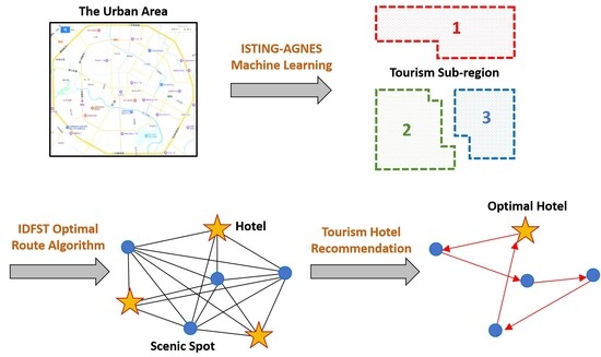
Tourism Hotel Recommendation Model Based on ISTING-AGNES Machine Learning and IDFST Optimal Route Algorithm

Abstract

To address the problem that hotel recommendations in tourism activities do not consider the spatial relationship between hotels and scenic spots and the cost of tour routes, we construct a tourism hotel recommendation model based on ISTING-AGNES machine learning and an IDFST optimal route algorithm. Firstly, a scenic spot spatial clustering model based on the ISTING-AGNES machine learning algorithm is constructed, including a scenic spot ISG spatial topological model based on the neighborhood cell growth algorithm and an ISTING-AGNES machine learning algorithm based on the scenic spot ISG spatial topological model, which can realize spatial dimension reduction in tourist cities and construct tourism sub-regions for recommending scenic spots and hotels. Secondly, taking the tourism sub-regions as the modeling scope, a tourism hotel recommendation model based on the IDFST optimal route algorithm is constructed in which a closeness model between the tourists’ interests and the attributes of scenic spots in the sub-region is established to recommend the most matched scenic spots for tourists. Then, based on the recommended scenic spots, a tourism sub-interval optimal route algorithm based on IDFST and a tourism hotel recommendation model based on the optimal route decision forest algorithm are established to search for the global optimal tour route—with hotels as the starting and ending points and scenic spots as nodes—and to recommend the hotel with the most cost-effective tour route for tourists. The experiments prove that the constructed algorithm can output the hotel with the best geospatial location and the lowest tour route cost. Under the experimental conditions, compared with the hotel recommended by the weighted centroid positioning algorithm, the cost optimization rate reaches 5.98%. Compared with the greedy mountain climbing algorithm and the greedy BFS algorithm, the cost optimization rates reach 14.73% and 16.03%, proving that the constructed algorithm is feasible and advantageous over the traditional algorithms.

1. Introduction

1.1. Research Background and Existing Problems

1.1.1. Research Background

Selecting a suitable hotel to check in and stay at for rest is an important part of travel itinerary planning. Tourists arriving at a tour destination from a tourist source city usually first check in at their reserved hotel before starting their travel itinerary. Therefore, when tourists make plans before traveling, they usually consider hotel selection as an important factor and reserve a hotel in advance. There are many factors that tourists consider when choosing a hotel, such as price, location, service, star rating, etc. Among many factors, one of the most important and crucial factors that tourists consider is the spatial relationship between hotels and scenic spots, usually the cost of distance. When tourists choose a hotel, they hope that the hotel location is at a close spatial distance to the scenic spots to be visited, in order to minimize the transportation and time costs from the hotel to the scenic spots and to spend as much time as possible visiting the scenic spots. Therefore, under conditions of a large coverage area and multiple scenic spots in a tourist city, providing tourists with scenic spots that match their interests and recommending hotels with the optimal spatial location, as well as minimizing the transportation and time costs for tourists to travel from hotels to scenic spots, are key factors to improve the overall efficiency of tourism and tourist satisfaction [1,2,3].

Based on the above research objectives, from the perspective of optimizing spatial relationships, the core essences of establishing a hotel recommendation model are as follows [4,5].

The first one is to identify representative scenic spots distributed in the tourist city, establishing spatial clustering relationships between scenic spots in order to determine the spatial distribution of the scenic spots and provide a spatial basis for establishing the hotel recommendation model. In the first step, it is necessary to establish the basic structure of the urban space, divide the urban space into small units, and form basic units covering the scenic spots. Then, a spatial clustering algorithm must be constructed to cluster the basic units containing the scenic spots. The distribution ranges of clusters form the urban tourism sub-regions, which contain representative scenic spots of different types and quantities. This process realizes dimensionality reduction in the whole urban tourism region, which can effectively reduce the spatial dimension and the complexity of the hotel recommendation algorithm.

The second one is to match and recommend scenic spots that meet the tourists’ interests within the tourism sub-region, and then determine the hotels that are distributed within the sub-region and meet the needs of tourists for accommodation. Firstly, the model needs to establish the closeness relationship between tourists’ interests and scenic spots and recommend the optimal scenic spots for tourists. Then, it must establish the spatial relationship between the hotels and recommended scenic spots in order to obtain the optimal hotel recommendation. This process takes into account the coordinate position, distance relationship, spatial distribution, and other factors between the hotels and scenic spots.

The third one is to conduct a deep integration of tourism scenes. Tourists depart from the hotel to visit scenic spots and then return to the hotel to rest after finishing their trip. When tourists are visiting a large number of scenic spots in a day, the model will form a certain order and route of sightseeing. The route connecting the hotel and scenic spots is a key factor in generating the transportation and time costs, and the core element determining the cost is the distance between the hotel and the scenic spots, as well as the overall travel route distance. Therefore, starting from the hotel, searching for the tour route with the optimal travel distance that connects the scenic spots can provide the optimal hotel recommendation.

1.1.2. Existing Problems

Based on the core essence of constructing a hotel recommendation model, we analyze the current research studies on hotel recommendation and the existing problems in recommendation methods [6,7,8]. The first one is that the mainstream research studies focus on using hotels themselves as the research objects, constructing the hotel attribute labels from the perspectives of accommodation condition, price, star rating, service, etc., and then establishing the user labels from the perspectives of the emotion, demand, and interest preference, constructing the matching relationship between the two factors, and recommending the most suitable hotel for users. This research method simply considers the issue from the perspective of the users’ accommodation in hotels, focusing on the service and evaluation of hotels, and recommending high-quality hotels as much as possible. However, it ignores its relationship with tourism and does not closely integrate hotel recommendation with tourist activities, making it unsuitable for tourism scenarios. The second one is to collect users’ needs and evaluations of the hotels through online reviews, and establish the connection between users and hotels. By constructing the statistical and sorting algorithms to rank the hotels, then recommend the best hotels to the users. This research method conducts the statistical analysis on users’ historical evaluation data without mining and matching the users’ current needs and interests. Although it can obtain a rough trend of interest matching from the statistical perspective, it cannot achieve the personalized recommendation. In addition, this research method does not combine tourist activities and does not consider the hotel recommendation in tourism scenarios. The third one is to use the conventional recommendation algorithms such as collaborative filtering to implement hotel recommendation, including content-based collaborative filtering, user-based collaborative filtering, and project-based collaborative filtering. These research methods are all approximate recommendations and do not recommend hotels based on the current users and tourism scenarios.

Through the analysis of the mainstream research methods mentioned above, it can be concluded that the current research studies on the hotel recommendation methods focus on the recommendation of hotel check-in selection, without deep integration with tourism scenarios. There is no research on hotel recommendation from the perspective of optimizing tourism space, optimizing tourism transportation costs, improving tourism efficiency, and enhancing tourists’ satisfaction. Especially when tourists need to stay at hotels with the optimal distance from the scenic spots in tourism scenarios, the current research methods cannot achieve the spatial optimization modeling, making it difficult to determine the optimal hotel location in space. There is also no optimization of tourism dimension, and no research on hotel recommendation from the perspective of reducing spatial dimension, while the mainstream research studies still consider the tourist city as a whole region for hotel recommendation. This not only requires a large amount of computation for recommendation algorithms, but also makes it difficult to achieve the optimal tourism transportation costs. In addition, implementing hotel recommendation through the construction of optimal route algorithm is currently not covered in research methods. The optimal tour route planning is a crucial aspect of the tourism planning. After checking into a hotel, tourists need to depart from the hotel to visit the scenic spots. When there are a large number of scenic spots, the tourism planning inevitably involves the arrangement of the tour route. Selecting a hotel from the perspective of optimizing the overall cost of the route is also a key factor that tourists should consider in their travel itinerary planning. However, current research studies on hotel recommendation do not construct the models from this perspective.

1.2. Research Objectives

Based on the analysis of research background and existing problems, we propose the following research objectives:

(1)

Research objective 1: Construct hotel recommendation model that integrates tourism scenario, combine tourism space optimizing, tourism transportation cost optimizing, tourism efficiency improving and tour route planning into the hotel recommendation model, recommending the optimal hotels for tourists and minimizing the transportation costs.

(2)

Research objective 2: Construct scenic spot spatial clustering model based on the ISTING-AGNES (Improved Statistical Information Grid–Agglomerative Nesting) machine learning algorithm, establish clustering relationship between scenic spots in the city, and divide the city into local spaces with clusters as the topological units according to the clustering algorithm. Each local space corresponds to a tourism sub-region, which contains different types of scenic spots. This method can reduce dimensionality of hotel recommendation and improve computational efficiency of the recommendation algorithm, and it can recommend scenic spots that meet tourists’ interests while also recommending hotels with the lowest transportation costs.

(3)

Research objective 3: Construct tourism hotel recommendation model based on the IDFST (improved depth first search tree) optimal route algorithm, and achieve spatial relationship modeling between hotels and the recommended scenic spots within a tourism sub-region. By establishing the IDFST optimal route algorithm that integrates hotels and the recommended scenic spots, it can output the hotel with the lowest transportation costs, effectively reducing tourists’ travel costs, improving tourism efficiency and tourists’ satisfaction.

1.3. Solutions and Research Architecture

Firstly, with regard to the research objective 1, we design the overall architecture of this work, as shown in Figure 1. A tourism hotel recommendation model based on the ISTING-AGNES machine learning and the IDFST optimal route algorithm is constructed, which includes two modules: a scenic spot spatial clustering model based on the ISTING-AGNES machine learning algorithm and a tourism hotel recommendation model based on the IDFST optimal route algorithm. By establishing a spatial clustering model and an optimal route algorithm, it achieves the optimal hotel recommendation, and minimizes tourism transportation costs.

Secondly, with regard to the research objective 2, we construct a scenic spot spatial clustering model based on the ISTING-AGNES machine learning algorithm, which includes two parts: a scenic spot ISG (Improve Spatial Grid) spatial topological model based on the neighborhood cell growth algorithm and an ISTING-AGNES clustering algorithm based on the scenic spot ISG spatial topological model. By using the neighborhood cell growth algorithm to construct the ISG spatial topological model containing scenic spots, and integrating the advantages of STING clustering algorithm and AGNES clustering algorithm, we construct an ISTING-AGNES clustering algorithm to achieve cell clustering and form tourism sub-regions. It performs dimensionality reduction on the urban tourism space, and can improve the efficiency of the hotel recommendation algorithm.

Finally, with regard to the research objective 3, we construct a tourism hotel recommendation model based on the IDFST optimal route algorithm, which includes three parts: a scenic spot recommendation model based on attribute closeness, a tourism sub-interval optimal route algorithm based on IDFST, and a tourism hotel recommendation model based on the optimal route decision forest algorithm. By searching for the tour routes composed of hotels and scenic spots within a tourism sub-region, it establishes the optimal tour route for the entire sub-region, recommends hotel with the lowest travel costs for tourists, minimizes the travel costs, and finally improves tourists’ satisfaction.

1.4. Main Contributions and Innovations

The main contributions and innovations of this work are as follows.

(1)

Aiming at the research background and the existing problems related to the hotel recommendation, an innovative hotel recommendation model integrating a tourism scenario is constructed. Unlike the traditional research methods, the hotel recommendation model constructed in this work deeply integrates the tourism scenario, incorporating the optimization of tourism space, optimization of tourism transportation costs, improvement in tourism efficiency, and planning of tour routes into the hotel recommendation model, recommending hotels to the tourists from the perspective of optimal tour costs.

(2)

A scenic spot spatial clustering model based on the ISTING-AGNES machine learning algorithm is constructed by combining the distribution of scenic spots in the city and the geospatial constraints. The advantages of STING and AGNES clustering algorithms are integrated, and scenic spots are included in spatial topological cells, ultimately forming the tourism sub-regions with clusters as the basic structure, achieving spatial dimensionality reduction of the tourist cities and improving the efficiency of the hotel recommendation algorithm. This is an innovative method in hotel recommendation algorithm research.

(3)

A tourism hotel recommendation model based on the IDFST optimal route algorithm is established, which matches tourists’ interests and recommends scenic spots within tourism sub-regions, searches for the optimal tour route that integrates hotels and scenic spots, minimizes tourists’ transportation costs, and improves tourism efficiency and tourists’ satisfaction. This method of constructing a hotel recommendation algorithm based on the cost of tour routes is an innovative research method.

2. Related Work

We analyze and compare the representative research literature on the background and problems related to the hotel recommendation. Liu et al. [9] created a hotel recommendation system that combined the online reviews and ratings with offline tour groups. A subgroup weight calculation method considering the online group size and offline social trust network was designed by predicting the travel types of commenters and clustering them. By considering the strength and order information by online to offline method to confirm attribute importance, personalized hotel recommendations were provided for the offline decision-makers, and the necessary guidance was provided for travel agencies and platforms to improve services. This research method was based on user comments and predicting user needs, analyzing the importance of the recommendation attributes from the perspective of user emotions, and achieving the personalized recommendations. But there was no integration of tourism scenario, and no consideration given to optimize tourism costs. Alghamdi [10] developed a new green hotel recommendation method using the text mining and the long short-term memory techniques, and used the spectral clustering algorithm to cluster users’ ratings of green hotels. The long short-term memory could better predict customers’ overall evaluations of green hotels, achieving higher accuracy in recommendations. This research method essentially still recommended hotels themselves, and the goal of the model was to improve recommendation accuracy rather than reduce travel costs. Alam et al. [11] proposed a framework for ranking hotels by analyzing customer reviews and nearby amenities, while incorporating ratings generated from user reviews and surrounding facilities. The effectiveness and applicability of the proposed framework were demonstrated through experiments using the datasets from online hotel booking platforms such as TripAdvisor and Booking. This research method was also based on user evaluation, without considering the constraints of the urban geographic space to establish the tourism scenario. Essentially, it still recommended hotels themselves, and historical user review data was used to recommend hotels without considering current users’ needs. Barliza et al. [12] proposed a hierarchical multicriteria hotel evaluation model that included the important hotel attributes and previous customer ratings of the hotel. A recommendation system called HR.LSP was proposed, which used the different hierarchical logic aggregation operators to implement hotel recommendations based on the logical preference scoring methods. This method essentially relied on the user historical evaluation data, rather than mining and recommending by current users’ needs, and did not combine the tourism scenario and the optimization goals of tourism costs. Wang et al. [13] proposed a hotel collaborative filtering recommendation algorithm, which mined users’ historical evaluations of hotels, used the HowNet sentiment dictionary and the manual annotation method to analyze the sentiment of comment statements, and generated hotel recommendation results based on users’ historical data of hotel selection. The essence of this research method was to mine the historical data and analyze users’ emotions, recommend hotels for current users, without considering the personalized needs of the current users, and without combining tourism scenario and the cost optimization goals. Hasane et al. [14] established a hotel recommendation system based on the collaborative filtering method, which was configured with the latest variant of CNN (CapsNet), to recommend the most suitable hotels based on the user collaboration. Based on analyzing user preferences, the recommendations were made by using the similarity index between ratings specified in the database. This method, combined with the collaborative filtering techniques in traditional recommendation algorithms, still relied on users’ historical evaluation data and did not take into account current users’ needs and tourism scenario. Cui et al. [15] regarded the probabilistic linguistic term set (PLTS) as a data statistical tool for describing user review information, and, based on the PLTS theory, proposed a hotel recommendation algorithm. It analyzed the online user reviews of hotels, used the probabilistic language cosine similarity to calculate the hotel similarity, and ranked recommended hotels based on similarity. This method also involved the statistical analysis of historical reviews to obtain the hotel rankings and recommendations, but it still did not take into account the optimization goals of tourism scenario and costs. Shambour et al. [16] proposed a fusion multicriteria user-item collaborative filtering recommendation algorithm, which utilized users’ multicriteria ratings and integrated the MC user-based collaborative filtering and the MC item-based collaborative filtering technologies to generate the personalized hotel recommendations. This study essentially established hotel recommendations based on user ratings through the collaborative filtering algorithms, without combining tourism space optimization and tour route cost optimization. It was still a method of recommending hotels themselves.

By comparing with representative baseline methods, it can be concluded that the constructed hotel recommendation algorithm has the following innovations:

(1)

Some traditional baseline methods took historical user interests, evaluations, ratings, and other information as important indicators, and built models based on historical data. This is the collaborative filtering recommendation method based on users or items, which is essentially approximate recommendation, not precise recommendation. The constructed hotel recommendation algorithm is based on current interests of tourists, accurately matching the best scenic spots for them, and based on the recommended scenic spots, recommending the hotel with the lowest cost of travel route for tourists with higher accuracy. From the aspect of optimizing travel costs, the constructed recommendation algorithm is innovative.

(2)

Certain traditional baseline methods took hotel accommodation conditions, star rating, online evaluation, etc., as important reference basis to recommend hotels with better stay experience for tourists. These recommendation methods did not consider hotels as the most important part of tour planning, and did not take into account the impact of hotel location on tour routes and travel costs. The constructed recommendation algorithm takes tour routes and travel costs as core conditions, recommending hotels with the lowest travel costs to tourists and improving their satisfaction. Therefore, the constructed recommendation model has innovative algorithmic mechanism.

(3)

Some traditional baseline methods did not consider spatial distribution and recommendation of scenic spots as key factors, while they filtered and recommended hotels from the entire urban spatial range, resulting in high algorithm complexity. The constructed recommendation model firstly achieves spatial dimensionality reduction by the ISTING-AGNES clustering algorithm, generating tourism sub-regions. Then, it recommends scenic spots and hotels to tourists in the tourism sub-regions, reducing the complexity of the algorithm and improving the efficiency and accuracy of the algorithm. This is an innovative method in the construction of a hotel recommendation model.

3. Methodology

3.1. Scenic Spot Spatial Clustering Model Based on ISTING-AGNES Machine Learning Algorithm

The tourist cities usually contain a large number of scenic spots, which are distributed in different geographical locations of the city and have attributes and spatial characteristics. The attribute features are used to describe tourism functions of scenic spots, such as travel time, travel expenses, star rating, popularity, etc. They are important factors in describing tourism value and emotions that scenic spots bring to the tourists, and are also important indicators for recommending scenic spots to the tourists. The spatial features are used to describe the location and distribution of scenic spots, characterize the spatial relationships between scenic spots and between scenic spots and hotels, and are important indicators for constructing spatial clusters. When using the attribute features of scenic spots to describe tourists’ interests, it is possible to determine their interest tendencies and the scenic spots they may be interested in, which may be distributed in different sub-regions of the city. When the tourists’ interest tendencies are determined, the smaller the area of the tourists’ interested scenic spots distribution, and the more they can reduce transportation costs and improve tourism efficiency within a limited time. Conversely, if the tourists’ interested scenic spots are distributed throughout the entire city region, the tourists will pay higher transportation and time costs. Therefore, under the constraints of the urban geographic space, clustering the scenic spots distributed in the city and constructing tourism sub-regions that contain a certain number of scenic spots can achieve dimensionality reduction in the tourism space and provide more efficient operating space for a hotel recommendation algorithm [17,18,19].

We construct a scenic spot spatial clustering model based on the ISTING-AGNES machine learning algorithm, aiming to model the clustering of scenic spots into the tourism sub-regions in the urban space. Firstly, we establish a scenic spot ISG spatial topological model based on the neighborhood cell growth algorithm, divide the city into micro cell grids to form cellular units, then construct the neighborhood cell growth algorithm to form the growth cells containing scenic spots, and further use topology to form the scenic spot ISG space. Secondly, by integrating the advantages of STING and AGNES clustering algorithms, an ISTING-AGNES clustering algorithm based on the scenic spot ISG spatial topological model is constructed to achieve the clustering of growth cells and form spatial clusters containing different scenic spots, corresponding to the formation of tourism sub-regions.

The theoretical analysis, innovation analysis, and originality analysis of the two modeling ideas are as follows:

(1)

The scenic spot ISG spatial topological model based on neighborhood cell growth algorithm. This model is an original model built on the basis of the STING algorithm, and we optimize and improve the STING clustering algorithm idea. The traditional STING clustering algorithm requires setting a density threshold, and deleting the sparse units during the clustering process can result in the loss of elements in the entire clustering space. The constructed ISTING algorithm has made significant improvements to the clustering process, dividing the urban space into grids that contain scenic spot elements. Topology generation of scenic spot cells is performed on the neighboring grids by using the grids that contain scenic spot elements. Based on the generated scenic spot cells, the topological algorithm is further constructed to generate the ISG space. This is a prerequisite for building a clustering algorithm, ensuring that each scenic spot element is a clustering target element.

(2)

The ISTING-AGNES clustering algorithm based on the scenic spot ISG spatial topological model. The constructed ISTING-AGNES clustering algorithm is an original algorithm that combines and optimizes the STING and AGNES clustering algorithms. On the basis of STING grid partitioning and generating spatial cells, the AGNES clustering algorithm is optimized and improved by using large-capacity cells as clustering centers and determining the number of clusters at a certain granularity. The position of the clustering center cell is determined by factors such as spatial distribution of scenic spots, granularity of clustering, and coverage area of travel sub-regions, which better match the geospatial conditions of the scenic spot and hotel recommendation algorithm. At the same time, in the design of the clustering algorithm, the objective function is calculated based on the cell spatial distribution, cell positioning centers, etc., avoiding the computational complexity of using the single scenic spot element to calculate the objective function while requiring multiple iterations. The efficiency of clustering algorithms is higher.

3.1.1. Scenic Spot ISG Spatial Topological Model Based on Neighborhood Cell Growth Algorithm

In data mining algorithms, the SG (Spatial Grid) model is a method for implementing spatial clustering, and its construction is based on regular grids. Due to the fact that the spatial scope represented by tourism sub-region in the city is composed of the multiple micro unit grids, we optimize the SG model and construct a neighborhood cell growth algorithm by using the micro unit grids to form the basic units for constructing the ISTING-AGNES clustering algorithm [20].

Definition 1.

Spatial delineation region  $S_c$ of tourist city and scenic spot element $T_{(i)}$. For a certain tourist city, we construct an $ma\times na$ area covering the entire main urban region of the city, and define this area as the spatial delineation region $S_c$ of the tourist city. We establish a coordinate system $xoy$ with the upper left corner of the region $S_c$ as the origin, where $a$ is the division step size of the region $S_c$ in the coordinate system $xoy$, $m$ is the total step size of the region $S_c$ on the $x$ axis, $n$ is the total step size of the region $S_c$ on the $y$ axis, and satisfies $m,n,a\in Z^{+}$. We define the scenic spots to be clustered distributed in the city as the scenic spot elements $T_{(i)}$. When the total number of scenic spots is $p$, it satisfies $0<i\le p$, $i,p\in Z^{+}$.

Definition 2.

Spatial cellular unit  $C_{e(i,j)}$ of tourist city. In the urban spatial coordinate system $xoy$, the $x$ axis and $y$ axis of the region $S_c$ are divided into units with a step size of $a$. If the $x$ axis is divided into $m$ units and the $y$ axis is divided into $n$ units, the entire region $S_c$ is divided into $m\times n$ units with an area of $a\times a$. One unit is defined as the spatial cellular unit $C_{e(i,j)}$ of the tourist city, where $i$ is the $x$ axis code of the coordinate system $xoy$ where the unit $C_{e(i,j)}$ is located, $j$ is the $y$ axis code of the coordinate system $xoy$ where the unit $C_{e(i,j)}$ is located, and satisfies $0<i\le m$, $0<j\le n$, $i,j,m,n\in Z^{+}$.

Definition 3.

Spatial operation matrix  ${\mathbf{M}}_{Sc}$ of tourist city. We use the division of $x$ axis and $y$ axis by unit step size $a$ in the coordinate system $xoy$ as the basic logic to construct a matrix with dimension $m\times n$ for storing the cellular units $C_{e(i,j)}$. This matrix is defined as the spatial operation matrix ${\mathbf{M}}_{Sc}$ of the tourist city. The element of the matrix is $M_{(i,j)}$, corresponding to the store cellular unit $C_{e(i,j)}$, satisfying $0<i\le m$, $0<j\le n$, $i,j,m,n\in Z^{+}$.

Definition 4.

Scenic spot growth cell  $G_{c(i)}$ and cell capacity $d_{(i)}$. Based on the constructed neighborhood cell growth algorithm, we take a certain scenic spot $T_{(i)}$ as the growth center point and establish a rectangular buffer zone around the center point, which contains no less than one scenic spot. The formed buffer zone containing certain scenic spots $T_{(i)}$ is defined as a scenic spot growth cell $G_{c(i)}$. When the number of growth cells $G_{c(i)}$ formed in region $S_c$ is $h$, there are $0<i\le h$, $i,h\in Z^{+}$. The number of scenic spots included in the growth cell $G_{c(i)}$ is defined as cell capacity $d_{(i)}$, which is the core indicator for constructing the clustering algorithm. According to the definition, the cell capacity $d_{(i)}$ and the total number $p$ of scenic spots in the region $S_c$ satisfy the relationship in Formula (1), $0<d_{(i)}<<p$, $d_{(i)},p\in Z^{+}$.

$${\displaystyle \sum _{i=1}^h{d}_{(i)}}=p$$

(1)

Definition 5.

Neighborhood topological cell  $G_{t(i)}$. According to Definition 4, when the area of the  $h$  growth cells  $G_{c(i)}$  exists,  ${\displaystyle {\sum }_{i=1}^{h}Area\left[G_{c(i)}\right]}<Area\left[S_c\right]$, and any adjacent cell  $\forall G_{c(i)}$  and  $\forall G_{c(j)}$  do not have a common edge, the cell formed by the boundary of cell  $G_{c(i)}$  and  $G_{c(j)}$  that does not contain scenic spots is defined as a neighborhood topological cell  $G_{t(i)}$. If a total of  $h^{*}$  cells  $G_{t(i)}$  are generated within region  $S_c$, then it satisfies Formula (2). According to a specific topological algorithm, the shape of the cell  $G_{t(i)}$  may be irregular.

$${\displaystyle {\displaystyle \sum _{i=1}^h}Area\left[G_{c(i)}\right]}+{\displaystyle {\displaystyle \sum _{i=1}^{h^{*}}}Area\left[G_{t(i)}\right]}=Area[S_c]$$

(2)

According to Definition 1 to Definition 5, we obtain the relationship diagram between each definition, as shown in Figure 2. Figure 2a shows the spatial delineation area $S_c$ established on the built-up area of a tourist city; Figure 2b shows the extracted scenic spot elements $T_{(i)}$, with the green dots representing scenic spots; Figure 2c shows the division of the $x$ axis and $y$ axis in the coordinate system $xoy$ with a step size of $a$, resulting in spatial unit cells $C_{e(i,j)}$ of the tourist city, as indicated by the yellow area in the figure; Figure 2d shows the constructed tourist city spatial operation matrix ${\mathbf{M}}_{Sc}$, with the gray areas representing matrix elements $M_{(i,j)}$; Figure 2e shows the scenic spot growth cells $G_{c(i)}$ generated on the basis of matrix ${\mathbf{M}}_{Sc}$, as indicated by the red area in the figure; Figure 2f shows the neighborhood topological cells $G_{t(i)}$ generated based on matrix ${\mathbf{M}}_{Sc}$ and cells $G_{c(i)}$, as shown in the blue area in the figure.

According to the definitions, we construct the scenic spot ISG spatial topological model based on the neighborhood cell growth algorithm, which includes Algorithms 1 and 2. The goal of Algorithm 1 is to construct the scenic spot growth cells in the coordinate system $xoy$, while the goal of Algorithm 2 is to establish the ISG spatial topological model based on the matrix ${\mathbf{M}}_{Sc}$ and the cells $G_{c(i)}$.

Algorithm 1: The Scenic Spot Growth Cell Algorithm based on the Cellular Center Point Topology
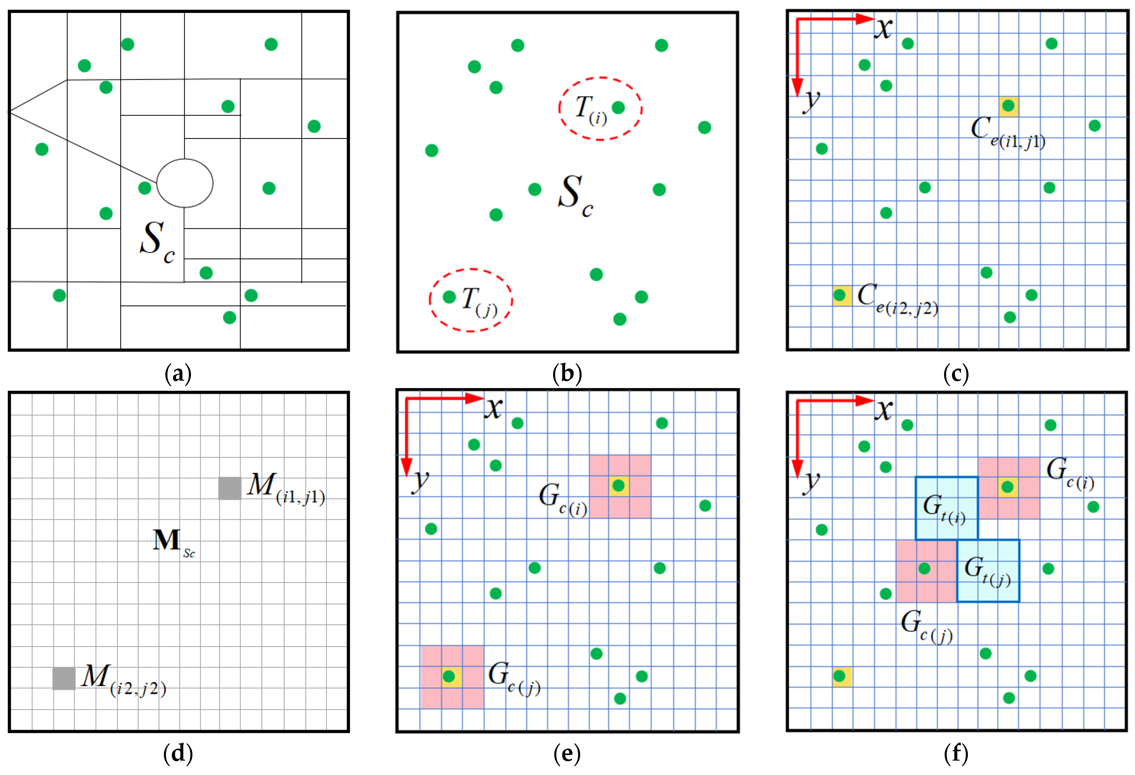
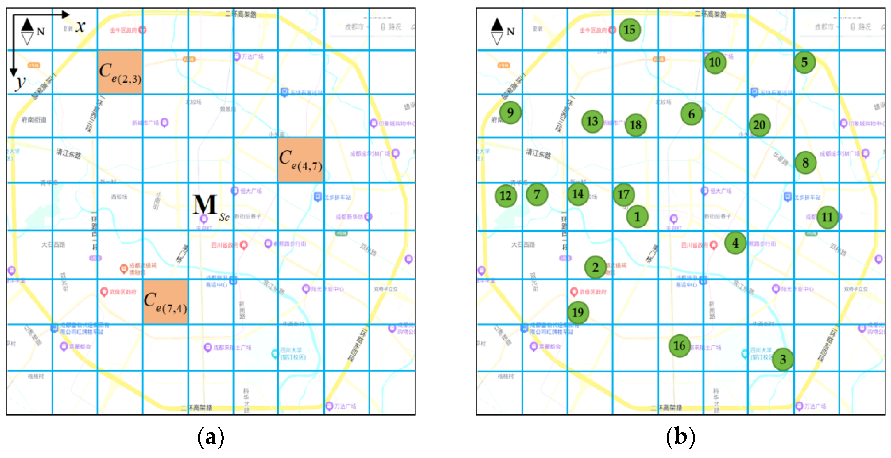
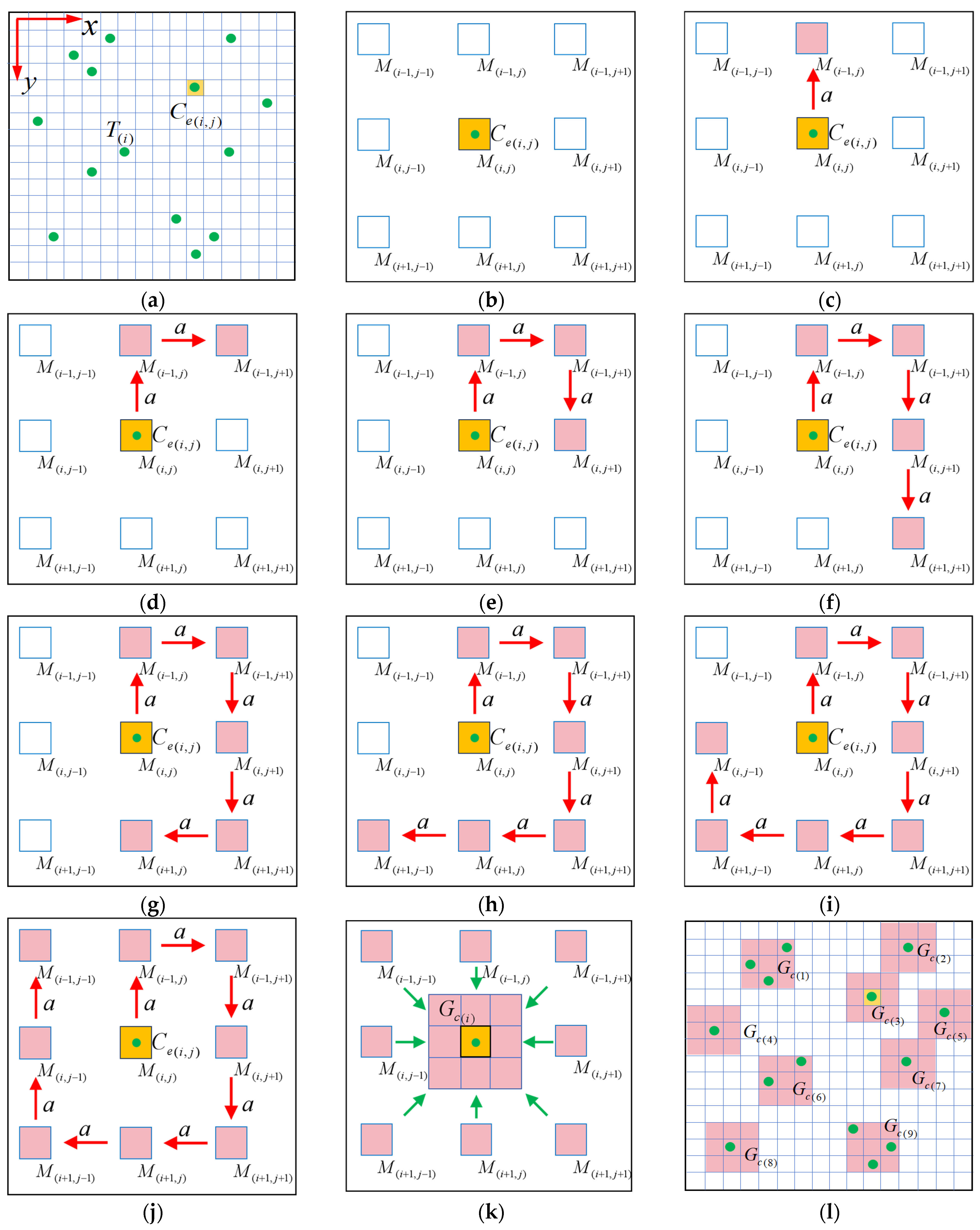
1:	Select the built-up area of a tourist city and delineate region $S_c.$ Establish the coordinate system $xoy$ for region $S_c$ and divide the $x$ axis and $y$ axis by step size $a$ to obtain a region with a dimension of $m\times n,$ as shown in Figure 3a. The green dots in the figure represent scenic spots, and the yellow grids represent cellular units $C_{e(i,j)}.$
2:	Establish matrix  ${\mathbf{M}}_{Sc}$ for storing the cells $C_{e(i,j)}$ with the dimension of $m\times n,$ and store the corresponding cells $C_{e(i,j)}$ in matrix elements $M_{(i,j)}.$
3:	Select arbitrary scenic spot  $\forall T_{(i1)}$ as the center point of the cell. The cell where the scenic spot  $\forall T_{(i1)}$ is located is  $C_{e(i,j)},$ and matrix element is  $M_{(i,j)}.$
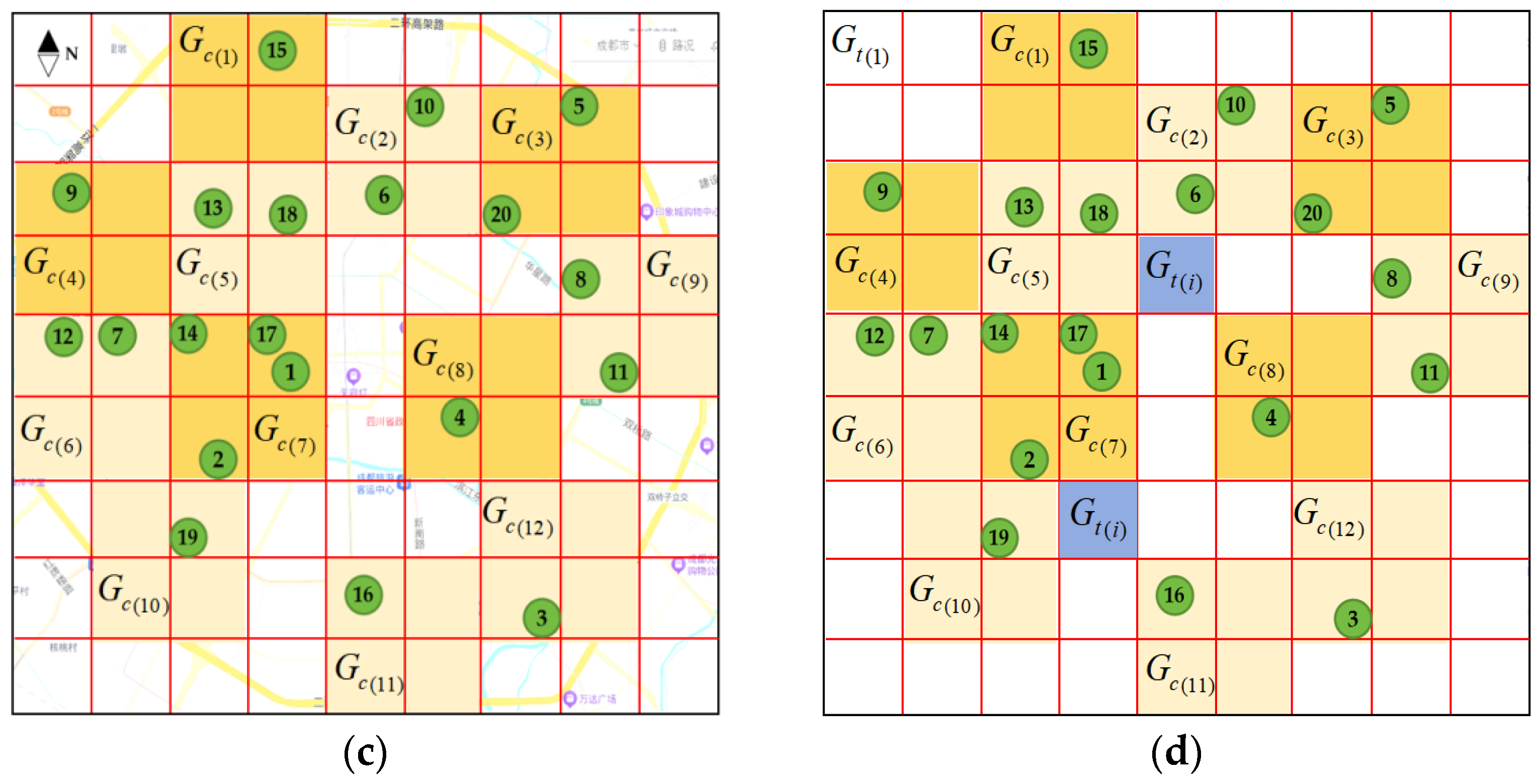
	(1)	Initialize the growth cell $G_{c(i)}$: {$M_{(i,j)}$} and cell capacity $d_{(i)}=1,$ as shown in Figure 3b, with the yellow cell $C_{e(i,j)}$ as the center point.
	(2)	Execute the step size $a$ find the element $M_{(i-1,j)},$ corresponding to the cell $C_{e(i-1,j)},$ and update $G_{c(i)}$: {$M_{(i,j)},$ $M_{(i-1,j)}$}, as shown in Figure 3c. Judge:
		①	If $C_{e(i-1,j)}\ne \varnothing ,$ then the cell contains a scenic spot, iterate and update $d_{(i)}=d_{(i)}+1;$
		②	If $C_{e(i-1,j)}=\varnothing ,$ there is no scenic spot in the cell, iterate and update $d_{(i)}=d_{(i)}+0.$
	(3)	Execute step size $a$ find element $M_{(i-1,j+1)},$ corresponding to cell $C_{e(i-1,j+1)},$ update $G_{c(i)}$: {$M_{(i,j)},$ $M_{(i-1,j)},$ $M_{(i-1,j+1)}$}, as shown in Figure 3d. Judge $C_{e(i-1,j+1)},$ iterate and update $d_{(i)}.$
	(4)	Execute step size $a$ find element $M_{(i,j+1)},$ corresponding to cell $C_{e(i,j+1)},$ update $G_{c(i)}$: {$M_{(i,j)},$ $M_{(i-1,j)},$ $M_{(i-1,j+1)},$ $M_{(i,j+1)}$}, as shown in Figure 3e. Judge $C_{e(i,j+1)},$ iterate and update $d_{(i)}.$
	(5)	Execute step size $a$ find element $M_{(i+1,j+1)},$ corresponding to cell $C_{e(i+1,j+1)},$ update $G_{c(i)}$: {$M_{(i,j)},$ $M_{(i-1,j)},$ $M_{(i-1,j+1)},$ $M_{(i,j+1)},$ $M_{(i+1,j+1)}$}, as shown in Figure 3f. Judge $C_{e(i+1,j+1)},$ iterate and update $d_{(i)}.$
	(6)	Execute step size $a$ find element $M_{(i+1,j)},$ corresponding to cell $C_{e(i+1,j)},$ update $G_{c(i)}$: {$M_{(i,j)},$ $M_{(i-1,j)},$ $M_{(i-1,j+1)},$ $M_{(i,j+1)},$ $M_{(i+1,j+1)},$ $M_{(i+1,j)}$}, as shown in Figure 3g. Judge $C_{e(i+1,j)},$ iterate and update $d_{(i)}.$
	(7)	Execute step size $a$ find element $M_{(i+1,j-1)},$ corresponding to cell $C_{e(i+1,j-1)},$ update $G_{c(i)}$: {$M_{(i,j)},$ $M_{(i-1,j)},$ $M_{(i-1,j+1)},$ $M_{(i,j+1)},$ $M_{(i+1,j+1)},$ $M_{(i+1,j)},$ $M_{(i+1,j-1)}$}, as shown in Figure 3h. Judge $C_{e(i+1,j-1)},$ iterate and update $d_{(i)}.$
	(8)	Execute step size $a$ find element $M_{(i,j-1)},$ corresponding to cell $C_{e(i,j-1)},$ update $G_{c(i)}$: {$M_{(i,j)},$ $M_{(i-1,j)},$ $M_{(i-1,j+1)},$ $M_{(i,j+1)},$ $M_{(i+1,j+1)},$ $M_{(i+1,j)},$ $M_{(i+1,j-1)},$ $M_{(i,j-1)}$}, as shown in Figure 3i. Judge $C_{e(i,j-1)},$ iterate and update $d_{(i)}.$
	(9)	Execute step size $a$ find element $M_{(i-1,j-1)},$ corresponding to cell $C_{e(i-1,j-1)},$ update $G_{c(i)}$: {$M_{(i,j)},$ $M_{(i-1,j)},$ $M_{(i-1,j+1)},$ $M_{(i,j+1)},$ $M_{(i+1,j+1)},$ $M_{(i+1,j)},$ $M_{(i+1,j-1)},$ $M_{(i,j-1)},$ $M_{(i-1,j-1)}$}, as shown in Figure 3j. Judge $C_{e(i-1,j-1)},$ iterate and update $d_{(i)}.$
	(10)	After searching all neighborhood cells $C_{e(x,y)},$ output growth cell $G_{c(i)}$ and cell capacity $d_{(i)},$ as shown in Figure 3k.
4:	Search for arbitrary scenic spot $\forall T_{(i2)},$ follow steps (1)–(10) in Step 3 to search for all neighborhood cells $C_{e(x,y)}$ of cell $C_{e(i,j)}$ where scenic spot $\forall T_{(i2)}$ is located, and output the growth cell $G_{c(i)}$ and cell capacity $d_{(i)}.$
5:	For scenic spot $\forall T_{(i)},$ traverse the $p$ scenic spots within region $S_c$ to obtain the $h$ scenic spot cells $G_{c(i)}$ and corresponding capacities $d_{(i)},$ $0<i\le p,$ $0<i\le p,$ $i,p\in Z^{+},$ as shown in Figure 3l.

Based on scenic spot growth cell $G_{c(i)}$, we use the matrix ${\mathbf{M}}_{Sc}$ searching method to construct a scenic spot ISG spatial model based on the cell topological algorithm in region $S_c$ of dimension $m\times n$. Starting from growth cell $G_{c(i)}$, the topology is applied to cell units $C_{e(i,j)}$ within cell $G_{c(i)}$ neighborhood, and the neighborhood topological cells $G_{t(i)}$ connected to cell $G_{c(i)}$ are constructed to form the ISG space.

Algorithm 2: The Scenic Spot ISG Spatial Model based on the Cell Topological Algorithm
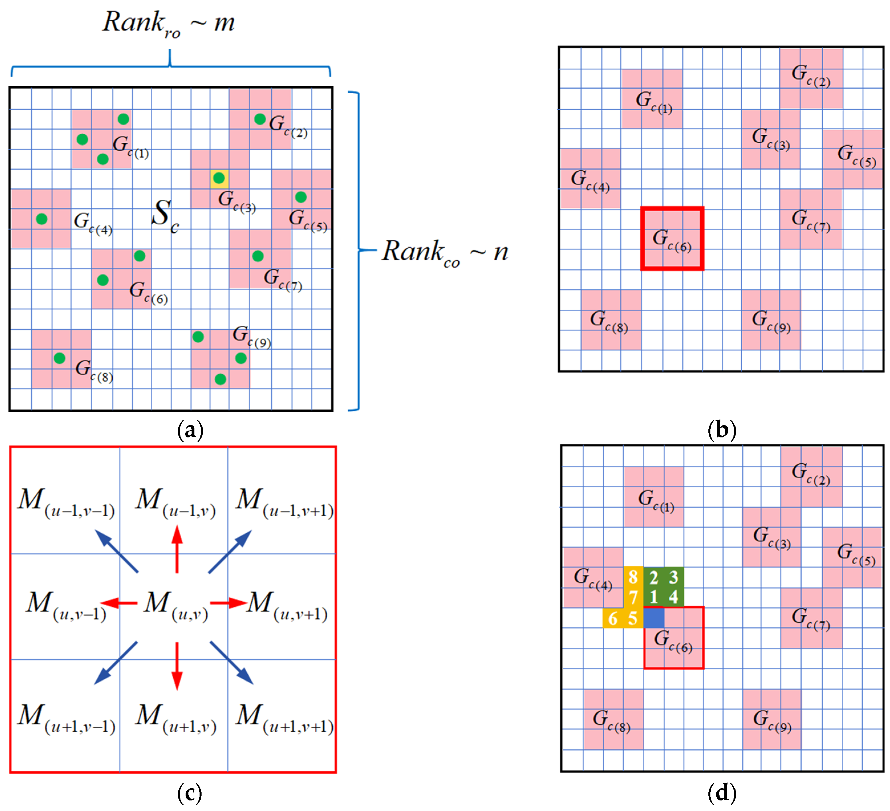
1:	Determine the $m\times n$ dimensional region $S_c$ and included $h$ number of scenic spot growth cells $G_{c(i)}.$ Determine the coordinate elements $M_{(i,j)}$ of cell units $C_{e(i,j)}$ contained in each cell $G_{c(i)}$ in matrix ${\mathbf{M}}_{Sc},$ as shown in Figure 4a.
2:	Select any cell $\forall G_{c(i)},$ as shown in the red box in Figure 4b. Define the local coordinates of matrix ${\mathbf{M}}_{Sc}$ within cell $G_{c(i)}$ as $M_{(u,v)},$ and label the coordinates of each cell unit $C_{e(u,v)},$ as shown in Figure 4c. Set the topology range as $2\times 2.$
3:	Select the coordinate $M_{(u-1,v-1)}$ and corresponding cell $C_{e(u-1,v-1)},$ as shown in the blue cell unit $C_{e(u-1,v-1)}$ within the red box cell in Figure 4d.
		(1)	Determine the adjacent cell $C_{e(u-2,v-1)}$ of the cell $C_{e(u-1,v-1)},$ namely, the No. 1 cell unit in Figure 4d, $C_{e(u-2,v-1)}=\varnothing ,$ and include it in the neighborhood topological cell $G_{t(1)};$
		(2)	Continue the topology and identify the adjacent cell $C_{e(u-3,v-1)}=\varnothing ,$ namely, the No. 2 cell unit in Figure 4d, and include it in the neighborhood topological cell $G_{t(1)};$
		(3)	Continue the topology and identify the adjacent cell $C_{e(u-3,v)}=\varnothing ,$ namely, the No. 3 cell unit in Figure 4d, and include it in the neighborhood topological cell $G_{t(1)};$
		(4)	Continue the topology and identify the adjacent cell $C_{e(u-2,v)}=\varnothing ,$ namely, the No. 4 cell unit in Figure 4d, and include it in the neighborhood topological cell $G_{t(1)};$ Form a $2\times 2$ dimensional topological cell $G_{t(1)}$ by No. 1 cell unit to No. 4 cell unit.
		(5)	Determine the current situation ${\displaystyle {\sum }_{i=1}^{h}Area[G_{c(i)}]}+Area\left[G_{t(1)}\right]<Area[S_c]$ and proceed to Step 4.
4:	Continue the topology outward with cell unit $C_{e(u-1,v-1)}$ to form a new topological cell $G_{t(2)}.$
		(1)	Determine the adjacent cell $C_{e(u-1,v-2)}=\varnothing ,$ namely, the No. 5 cell unit in Figure 4d, and include it in the neighborhood topological cell $G_{t(2)};$
		(2)	Determine the adjacent cell $C_{e(u-1,v-3)}=\varnothing ,$ namely, the No. 6 cell unit in Figure 4d, and include it in the neighborhood topological cell $G_{t(2)};$
		(3)	Determine the adjacent cell $C_{e(u-2,v-3)}\ne \varnothing ,$ delete it;
		(4)	Determine the adjacent cell $C_{e(u-2,v-2)}=\varnothing ,$ namely, the No. 7 cell unit in Figure 4d, and include it in the neighborhood topological cell $G_{t(2)};$
		(5)	Determine the adjacent cell $C_{e(u-3,v-2)}=\varnothing ,$ namely, the No. 8 cell unit in Figure 4d, and include it in the neighborhood topological cell $G_{t(2)};$ Form a $2\times 2$ dimensional topological cell $G_{t(2)}$ by No. 5 cell unit to No. 8 cell unit.
		(6)	Determine the current situation ${\displaystyle {\sum }_{i=1}^{h}Area[G_{c(i)}]}+{\displaystyle {\sum }_{i=1}^{2}Area[G_{t(i)}]}<Area[S_c]$ and proceed to the Step 5.
5:	Continue the topology of the cell unit $C_{e(x,y)}=\varnothing$ by using the same method as Step 3 to Step 4, and determine the following:
		(1)	If the current topology state satisfies ${\displaystyle {\sum }_{i=1}^{h}Area[G_{c(i)}]}+{\displaystyle {\sum }_{i=1}^{h^{*}}Area\left[G_{t(i)}\right]}<Area[S_c],$ continue the topology;
		(2)	If the current topology state satisfies ${\displaystyle {\sum }_{i=1}^{h}Area[G_{c(i)}]}+{\displaystyle {\sum }_{i=1}^{h^{*}}Area\left[G_{t(i)}\right]}=Area[S_c],$ the topology ends, and the ISG space consisting of $h$ scenic spot growth cells $G_{c(i)}$ and $h^{*}$ neighborhood topological cells $G_{t(i)}$ is output.

3.1.2. The ISTING-AGNES Clustering Algorithm Based on Scenic Spot ISG Spatial Topological Model

In the process of constructing the ISG spatial model, the algorithm divides urban region $S_c$ into $h$ number of scenic spot growth cells $G_{c(i)}$ and $h^{*}$ number of neighborhood topological cells $G_{t(i)}$, which are key elements for constructing spatial clusters. To achieve accurate recommendations of scenic spots and hotels and minimize the travel transportation costs for tourists, it is necessary to further divide the urban region into tourism sub-regions and recommend scenic spots within these sub-regions to determine the optimal hotel location. The construction of tourism sub-regions needs to meet the following conditions:

(1)

Deeply integrating tourism conditions, using geospatial distribution of scenic spots as the dividing standard;

(2)

The number of sub-regions ≥ 2;

(3)

Within the sub-region: the number of scenic spots $T_{(i)}$ ≥ 1, and the number of hotels $H_{(i)}$ ≥ 1;

(4)

Arbitrary sub-region covers a certain area and there is no overlap area;

(5)

The sum of the areas of all sub-regions is equal to the total area of the region $S_c$.

Under the constraints of the above conditions, we construct an ISTING-AGNES clustering algorithm based on the ISG spatial topological model by the basic elements of $h$ number of scenic spot growth cells $G_{c(i)}$ and $h^{*}$ number of neighborhood topological cells $G_{t(i)}$. The region $S_c$ is divided into tourism sub-regions with the spatial clusters as the basic structure. In clustering algorithms, STING is a grid-based spatial clustering method, while AGNES is a bottom-up hierarchical clustering algorithm, both of which have advantages and characteristics. We combine the advantages of STING and AGNES to construct the ISTING-AGNES clustering algorithm [21].

Definition 6.

Cluster initial Open List and cluster termination Closed List. Based on the constructed ISG model, the  $h$ number of the scenic spot growth cells  $G_{c(i)}$  and  $h^{*}$  number of the neighborhood topological cells  $G_{t(i)}$  generated in the ISG space are stored in the Open List as the initial dataset for clustering algorithm execution. When the clustering algorithm terminates, the  $h$  number of scenic spot growth cells  $G_{c(i)}$  and  $h^{*}$  number of neighborhood topological cells  $G_{t(i)}$  are stored in the Closed List. The data structure of the Open List and the Closed List are matrix  $M_{op}$  and matrix  $M_{cl}$  with the dimension  $2\times \max (h,h^{*})$. According to the definition, its storage structure satisfies the following conditions:

(1) 

The first row of the matrix stores the $h$ number of scenic spot growth cells $G_{c(i)}$, and the second row stores the $h^{*}$ number of neighborhood topological cells $G_{t(i)}$.

(2) 

The row rank of the matrix satisfies $ran{k}_{ro}=2$, and the column rank of the matrix satisfies $ran{k}_{co}=\max (h,h^{*})$.

(3) 

For the rows with fewer stored cells, the first element to the No.  $\min (h,h^{*})$  element stores the cells with corresponding attribute.

(4) 

For the rows with fewer stored cells, the value 0 is stored from the No.  $\min (h,h^{*})+1$  element to the No.  $\max (h,h^{*})$  element.

(5) 

The rows of the matrix are non-linearly correlated.

Definition 7.

Location center  $C_{Gc(i)}$ of scenic spot growth cell, longitude coordinate $L_{Gc(i)}$ of scenic spot growth cell, latitude coordinate $B_{Gc(i)}$ of scenic spot growth cell. Take arbitrary scenic spot growth cell $\forall G_{c(i)}$ with capacity of $d_{(i)}$. In urban geographic space environment, set the longitude and latitude of any scenic spot $T_{(i)}$ contained in the cell $G_{c(i)}$ as $l_{T(i)}$ and $b_{T(i)}$, and define the geometric center of $d_{(i)}$ number of scenic spots as the location center $C_{Gc(i)}$ of the scenic spot growth cell. Its longitude coordinate is $L_{Gc(i)}$, and its latitude coordinate is $B_{Gc(i)}$. Formula (3) is the constructed latitude and longitude model for the growth cells of scenic spots. The point with the coordinates ($L_{Gc(i)}$, $B_{Gc(i)}$) is the location center $C_{Gc(i)}$ of the scenic spot growth cell, which is used to measure the position of the cell $G_{c(i)}$ in the region $S_c$.

$$L_{Gc(i)}={\displaystyle \frac{1}{d_{(i)}}}\times {\displaystyle \sum _{i=1}^{d_{(i)}}{l}_{T(i)}}, B_{Gc(i)}={\displaystyle \frac{1}{d_{(i)}}}\times {\displaystyle \sum _{i=1}^{d_{(i)}}{b}_{T(i)}}$$

(3)

Definition 8.

Clustering objective function  $f(G_{c(i)},G_{c(j)})$ and normalization factor $\delta$. When constructing a clustering algorithm, the standard function for measuring the closeness between any scenic spot growth cells $\forall G_{c(i)}$ and $\forall G_{c(j)}$ is defined as the clustering objective function $f(G_{c(i)},G_{c(j)})$. It is measured by the straight-line distance between two points or the distance of traffic routes between two points. Here, as the location point of the cell $G_{c(i)}$ is determined by the geometric center of $d_{(i)}$ number of scenic spots $T_{(i)}$, which is not a solid point, the Euclidean distance between the two points is used as the basic model for constructing the clustering objective function, and the clustering objective function is established as shown in Formula (4). To constrain the clustering objective function value within the range of (0,1), we introduce the normalization factor $\delta$.

$$f(G_{c(i)},G_{c(i)})=\delta \times {\displaystyle \frac{1}{\sqrt{{\left(L_{Gc(i)}-L_{Gc(j)}\right)}^2+{\left(B_{Gc(i)}-B_{Gc(j)}\right)}^2}}}$$

(4)

We conduct in-depth analysis on the constructed clustering objective function.

Firstly, in Formula (4), we use Euclidean distance instead of urban road distance to construct the clustering objective function. The reasons for this are analyzed as follows:

(1)

Determined by the goal achieved by the algorithm. The goal in constructing the ISTING-AGNES clustering algorithm is to perform dimensionality reduction operations on high-dimensional urban space, thereby reducing the complexity of spatial search in the recommendation algorithm. The dimensionality reduction here refers to dividing the entire urban space into adjacent small areas, namely, tourism sub-regions. The way to achieve this goal is to build an ISTING-AGNES clustering algorithm. From the perspective of geospatial division, the algorithm only needs to implement area division and evenly group the scenic spots in the city into different sub-regions, so there is no need for complex road distance measurement. It only needs to construct a straight line distance based on the clustering center as the standard.

(2)

Determined by the algorithm complexity. The construction of road networks in cities is very mature, including a large number of roads and road nodes. In Section 3.2 and Section 4.2, by modeling, electronic map calculation, and on-site road distance collection, we obtain that the spatial distance between any scenic spot or hotel is positively correlated with the road distance. The larger the spatial distance is, the greater the road distance will be, and the smaller the spatial distance is, the smaller the road distance will be. This result indicates that using Euclidean distance to construct the objective function can ensure the stability of clustering results and is not affected by the road network distance. Meanwhile, using Euclidean distance can meet the modeling requirements when constructing a clustering algorithm, and the computational complexity is smaller, making the algorithm more efficient. If road distance is used for calculation, it will greatly increase the algorithm complexity.

(3)

Determined by the urban shape and spatial distribution. To achieve optimal hotel recommendations and reduce tourism transportation costs, the sub-regions generated by the clustering algorithm should be the continuous, adjacent, and evenly distributed planar regions. Using Euclidean distance to construct the clustering algorithm can generate uniform cluster shapes and effectively avoid irregular sub-regions formed by road bends, polylines, and other shapes.

Secondly, the constructed objective function plays a crucial role in optimizing the clustering algorithm and is the core element of constructing the ISTING-AGNES algorithm, mainly reflected in the following aspects:

(1)

The constructed objective function takes the cell localization center as the reference point, avoiding the computational complexity of using a single scenic spot element to calculate objective function while requiring multiple iterations. This is an optimization of the clustering algorithm mechanism, making the clustering algorithm more efficient.

(2)

In terms of clustering center selection, we avoid the traditional AGNES iterative search method and aim to generate uniformly distributed tourism sub-regions in urban space. We select cells with larger capacity and distributed in different geographical locations as clustering centers, and then calculate the objective function. This method greatly optimizes AGNES, reduces the computational complexity of the algorithm, and can obtain clusters with uniform spatial distributions.

(3)

We use objective function and spatial distribution of cells to determine clustering center cells, so the convergence speed of the clustering algorithm is extremely fast, which can quickly determine the center, position, and distribution range of each cluster without the complex process of multiple iterations. After determining the clustering centers, the other non-central cells could be directly determined for their closeness degrees with each center through the objective function, thus quickly confirming the clusters they should belong to. This further reduces the algorithm complexity and optimizes the clustering algorithm.

Definition 9.

Cluster center cell  $G_{c(i)}^{\mathrm{\Delta }}$ and cluster member cell  $G_{c(i)}^{*}$. According to the characteristics of the STING clustering algorithm, the core cell that represents the cluster determined by the algorithm is defined as the cluster center cell  $G_{c(i)}^{\mathrm{\Delta }}$, and the other remaining cell absorbed in the cluster is defined as the cluster member cell  $G_{c(i)}^{*}$. The cluster center cell  $G_{c(i)}^{\mathrm{\Delta }}$  and cluster member cell  $G_{c(i)}^{*}$  are both the elements of cluster.

Definition 10.

Cell cluster  $C_{(i)}$, cluster capacity $m_{(i)}$, clustering decision tree $Tre{e}_{(u)}$. The cell $G_{c(i)}$ gathering space generated by the clustering algorithm in the ISG space with a certain range is defined as cell cluster $C_{(i)}$, and the number of the generated clusters is denoted as $k$, $0<i\le k$, $i,k\in Z^{+}$. The total number of the cells $G_{c(i)}$ contained in a cluster $C_{(i)}$ is defined as cluster capacity $m_{(i)}$, and the total number of the cells $G_{c(i)}$ in the ISG space is $h$, $0<m_{(i)}\le h$. The criterion for any cell $\forall G_{c(i)}$ in the ISG space to be included in a cluster $C_{(i)}$ is the closeness between the cell $G_{c(i)}$ and the central cell $G_{c(i)}^{\mathrm{\Delta }}$ of the cluster $C_{(i)}$. When there are $k$ number of clusters and central cells $G_{c(i)}^{\mathrm{\Delta }}$ in the ISG space, the cell $G_{c(i)}$ and each cluster will generate $k$ number of clustering objective function values $f(G_{c(i)},G_{c(i)}^{\mathrm{\Delta }})$. By using the maximum decision tree algorithm to store the $k$ number of clustering objective function values into a complete binary tree, this tree is defined as the clustering decision tree $Tre{e}_{(u)}$.

According to the definition of the cluster, cluster $C_{(i)}$ meets the following conditions:

(1)

$C_{(i)}\ne \varnothing$, the cluster contains at least one cell;

(2)

Arbitrary $\forall C_{(i)}$ satisfies $\forall C_{(i)}\cap \forall C_{(j)}=\varnothing$;

(3)

$C_{(1)}\cup C_{(2)}\cup \dots \cup C_{(k)}=\left\{G_{c(i)}\right\}$;

(4)

$\forall C_{(i)}\ne \left\{G_{c(i)}\right\}$.

According to the definition of the clustering decision tree, the tree $Tre{e}_{(u)}$ satisfies the following conditions:

(1)

A completely binary tree structure with node encoding $t_{(x,y)}$. Among them, $x$ represents the layer of the tree, $y$ represents the No. $y$ node of layer $x$.

(2)

The root node is the first layer; when $y\ge 1$, the No. $x$ layer contains $2^{x-1}$ number of nodes.

(3)

Any node $t_{(x,y)}$ can have a maximum of 2 child nodes $t_{(x+1,*)}$ and a minimum of no node.

(4)

For any layer $\forall x$ and $\forall x+1$, the node storage value must meet $t_{(x,*)}{t}_{(x+1,*)}$.

(5)

For any layer $\forall x$, the node storage value must satisfy $t_{(x,y)}\ge t_{(x,z)}$, and $z\ge y$.

(6)

If No. $x$ layer has branch nodes, they are all concentrated on the leftmost side of the tree.

Definition 11.

Clustering matrix  $M_{C(i)}$. Cluster  $C_{(i)}$  that is generated by the cluster initial Open List and clustering algorithm is stored in a matrix according to certain rules, and the matrix is defined as clustering matrix  $M_{C(i)}$. Clustering matrix  $M_{C(i)}$  is the direct result of the clustering algorithm, which can visualize the location, distribution and clusters of the cells  $G_{c(i)}$  in the ISG space. The storage structure of matrix  $M_{C(i)}$  satisfies the following conditions:

(1) 

The dimension of the matrix is  $k\times \max m_{(i)}$, and  $k$  is the number of clusters and  $\max m_{(i)}$  is the maximum cluster capacity;

(2) 

Any row  $\forall x$  of the matrix stores a cluster  $C_{(i)}$,  $0<i\le k$,  $i,k\in Z^{+}$. The first element  $M(x,1)$  of the row stores the central cell  $G_{c(i)}^{\mathrm{\Delta }}$  of the cluster, while the other elements  $M(x,y)$  store the cluster member cells  $G_{c(i)}^{*}$,  $1<y\le m_{(i)}$,  $y,m_{(i)}\in Z^{+}$  ;

(3) 

Both the row rank and the column rank are full rank, that is,  $ran{k}_{ro}=k$,  $ran{k}_{co}=\max m_{(i)}$  ;

(4) 

In any row  $\forall x$, the front  $m_{(i)}$  number of elements store all the cells  $G_{c(i)}$  of the cluster  $C_{(i)}$, while the last  $\max m_{(i)}-m_{(i)}$  number of elements store the 0.

Based on Definition 6 to Definition 11 and the ISG spatial model, we construct an ISTING-AGNES clustering algorithm to cluster scenic spot growth cells $G_{c(i)}$ in the ISG space.

Step 1: Establish the cluster initial Open List and the cluster termination Closed List. According to the storage format of the List, store the $h$ number of scenic spot growth cells $G_{c(i)}$ and $h^{*}$ number of neighborhood topological cells $G_{t(i)}$ in the Open List.

Step 2: Scan the first row of the Open List and perform the following steps on the $h$ number of scenic spot growth cells $G_{c(i)}$:

(1)

Obtain the capacity $d_{(i)}$ of each scenic spot growth cell $G_{c(i)}$;

(2)

Sort the capacities $d_{(i)}$ by the maximum heap;

(3)

Take the front $k$ number of maximum values $\max d_{(i)}$ from the largest heap;

(4)

The corresponding cells $G_{c(i)}$ of the $k$ number of maximum values $\max d_{(i)}$ are the cluster center cells $G_{c(i)}^{\mathrm{\Delta }}$, $0<i\le k$, $i,k\in Z^{+}$. Store them into each first row element $M(x,1)$ of the matrix $M_{C(i)}$;

(5)

Delete the corresponding cells $G_{c(i)}$ of the $k$ number of maximum values $\max d_{(i)}$ from the Open List and store them in the Closed List.

Step 3: Note the remaining $h-k$ number of scenic spot growth cells $G_{c(i)}$ in the first row of the Open List as cluster member cells $G_{c(i)}^{*}$, then the encoding satisfies $0<i\le h-k$, $i,h-k\in Z^{+}$. Calculate the positioning centers $C_{Gc(i)}$ and the coordinates of the $k$ number of cluster center cells $G_{c(i)}^{\mathrm{\Delta }}$ and $h-k$ number of the cluster member cells $G_{c(i)}^{*}$.

(1)

Take the $d_{(i)}$ number of scenic spots $T_{(i)}$ stored within the $k$ number of cluster center cells $G_{c(i)}^{\mathrm{\Delta }}$ and $h-k$ number of cluster member cells $G_{c(i)}^{*}$;

(2)

Search for the longitude $l_{T(i)}$ and latitude $b_{T(i)}$ of scenic spots $T_{(i)}$ within each cell;

(3)

Calculate the longitude coordinate $L_{Gc(i)}$ and the latitude coordinate $B_{Gc(i)}$ of each cell;

(4)

Output the positioning center $C_{Gc(i)}$ of each cell.

Step 4: Build a complete binary tree $Tre{e}_{(u)}$ with a total number of $k$ nodes and initialize the heap $Tre{e}_{(u)}=0$. Take any cell $\forall G_{c(i)}^{*}$ from $h-k$ number of cluster member cells $G_{c(i)}^{*}$ and perform the following steps:

(1)

Take the first central cell $G_{c(1)}^{\mathrm{\Delta }}$ and calculate clustering objective function $f(G_{c(i)}^{*},G_{c(1)}^{\mathrm{\Delta }})$;

(2)

Take the second central cell $G_{c(2)}^{\mathrm{\Delta }}$ and calculate clustering objective function $f(G_{c(i)}^{*},G_{c(2)}^{\mathrm{\Delta }})$;

(3)

Comparison results:

(i)

If $f(G_{c(i)}^{*},G_{c(1)}^{\mathrm{\Delta }})>f(G_{c(i)}^{*},G_{c(2)}^{\mathrm{\Delta }})$, store $G_{c(1)}^{\mathrm{\Delta }}$ and $G_{c(2)}^{\mathrm{\Delta }}$ into nodes $t_{(1,1)}$ and $t_{(2,1)}$ of $Tre{e}_{(u)}$;

(ii)

If $f(G_{c(i)}^{*},G_{c(1)}^{\mathrm{\Delta }})\le f(G_{c(i)}^{*},G_{c(2)}^{\mathrm{\Delta }})$, store $G_{c(1)}^{\mathrm{\Delta }}$ and $G_{c(2)}^{\mathrm{\Delta }}$ into nodes $t_{(2,1)}$ and $t_{(1,1)}$ of $Tre{e}_{(u)}$;

(4)

Take the third central cell $G_{c(3)}^{\mathrm{\Delta }}$ and calculate clustering objective function $f(G_{c(i)}^{*},G_{c(3)}^{\mathrm{\Delta }})$, compare the results:

(i)

If $f(G_{c(i)}^{*},G_{c(1)}^{\mathrm{\Delta }})>f(G_{c(i)}^{*},G_{c(2)}^{\mathrm{\Delta }})$:

①

If $f(G_{c(i)}^{*},G_{c(3)}^{\mathrm{\Delta }})\ge f(G_{c(i)}^{*},G_{c(1)}^{\mathrm{\Delta }})>f(G_{c(i)}^{*},G_{c(2)}^{\mathrm{\Delta }})$, store $G_{c(1)}^{\mathrm{\Delta }}$, $G_{c(2)}^{\mathrm{\Delta }}$ and $G_{c(3)}^{\mathrm{\Delta }}$ into nodes $t_{(2,1)}$, $t_{(2,2)}$ and $t_{(1,1)}$ of $Tre{e}_{(u)}$;

②

If $f(G_{c(i)}^{*},G_{c(1)}^{\mathrm{\Delta }})>f(G_{c(i)}^{*},G_{c(3)}^{\mathrm{\Delta }})\ge f(G_{c(i)}^{*},G_{c(2)}^{\mathrm{\Delta }})$, store $G_{c(1)}^{\mathrm{\Delta }}$, $G_{c(2)}^{\mathrm{\Delta }}$ and $G_{c(3)}^{\mathrm{\Delta }}$ into nodes $t_{(1,1)}$, $t_{(2,2)}$ and $t_{(2,1)}$ of $Tre{e}_{(u)}$;

③

If $f(G_{c(i)}^{*},G_{c(1)}^{\mathrm{\Delta }})>f(G_{c(i)}^{*},G_{c(2)}^{\mathrm{\Delta }})>f(G_{c(i)}^{*},G_{c(3)}^{\mathrm{\Delta }})$, store $G_{c(1)}^{\mathrm{\Delta }}$, $G_{c(2)}^{\mathrm{\Delta }}$ and $G_{c(3)}^{\mathrm{\Delta }}$ into nodes $t_{(1,1)}$, $t_{(2,1)}$ and $t_{(2,2)}$ of $Tre{e}_{(u)}$.

(ii)

If $f(G_{c(i)}^{*},G_{c(1)}^{\mathrm{\Delta }})\le f(G_{c(i)}^{*},G_{c(2)}^{\mathrm{\Delta }})$:

①

If $f(G_{c(i)}^{*},G_{c(3)}^{\mathrm{\Delta }})<f(G_{c(i)}^{*},G_{c(1)}^{\mathrm{\Delta }})\le f(G_{c(i)}^{*},G_{c(2)}^{\mathrm{\Delta }})$, store $G_{c(1)}^{\mathrm{\Delta }}$, $G_{c(2)}^{\mathrm{\Delta }}$ and $G_{c(3)}^{\mathrm{\Delta }}$ into nodes $t_{(2,1)}$, $t_{(1,1)}$ and $t_{(2,2)}$ of $Tre{e}_{(u)}$;

②

If $f(G_{c(i)}^{*},G_{c(1)}^{\mathrm{\Delta }})\le f(G_{c(i)}^{*},G_{c(3)}^{\mathrm{\Delta }})\le f(G_{c(i)}^{*},G_{c(2)}^{\mathrm{\Delta }})$, store $G_{c(1)}^{\mathrm{\Delta }}$, $G_{c(2)}^{\mathrm{\Delta }}$ and $G_{c(3)}^{\mathrm{\Delta }}$ into nodes $t_{(2,2)}$, $t_{(1,1)}$ and $t_{(2,1)}$ of $Tre{e}_{(u)}$;

③

If $f(G_{c(i)}^{*},G_{c(1)}^{\mathrm{\Delta }})\le f(G_{c(i)}^{*},G_{c(2)}^{\mathrm{\Delta }})<f(G_{c(i)}^{*},G_{c(3)}^{\mathrm{\Delta }})$, store $G_{c(1)}^{\mathrm{\Delta }}$, $G_{c(2)}^{\mathrm{\Delta }}$ and $G_{c(3)}^{\mathrm{\Delta }}$ into nodes $t_{(2,2)}$, $t_{(2,1)}$ and $t_{(1,1)}$ of $Tre{e}_{(u)}$.

(5)

Use the same algorithm as steps (1)–(4), take the No. $i$ center cell $G_{c(i)}^{\mathrm{\Delta }}$, calculate clustering objective function $f(G_{c(i)}^{*},G_{c(i)}^{\mathrm{\Delta }})$, compare $f(G_{c(i)}^{*},G_{c(1)}^{\mathrm{\Delta }})$~$f(G_{c(i)}^{*},G_{c(i)}^{\mathrm{\Delta }})$, and store the $i$ number of function values into the previous $i$ number of nodes $t_{(x,y)}$ of $Tre{e}_{(u)}$. Traverse $i~(3,k]\in Z^{+}$, output a full rank tree $Tre{e}_{(u)}$ when the cell $G_{c(i)}^{\mathrm{\Delta }}$($i=k$) is traversed.

(6)

Take the root node $t_{(1,1)}$ of $Tre{e}_{(u)}$, and its stored cell $G_{c(i)}^{\mathrm{\Delta }}$ is the central cell of the cluster to which the selected cluster member cell $G_{c(i)}^{*}$ belongs. Include the $G_{c(i)}^{*}$ into the corresponding cluster $C_{(i)}$, and store the $G_{c(i)}^{*}$ into the related row of the cluster $C_{(i)}$ in matrix $M_{C(i)}$.

(7)

Delete the cell $G_{c(i)}^{*}$ from the Open List and store it in the Closed List.

Step 5: Return to Step 4 and continue to perform the steps with the same algorithm:

(1)

For $h-k$ number of cluster member cells $G_{c(i)}^{*}$, traverse $i~(0,h-k]\in Z^{+}$;

(2)

Calculate the cluster $C_{(i)}$ where the cell $G_{c(i)}^{*}$ is located and include $G_{c(i)}^{*}$ in the corresponding cluster $C_{(i)}$;

(3)

Store $G_{c(i)}^{*}$ into the row where the cluster $C_{(i)}$ is located in matrix $M_{C(i)}$;

(4)

Delete the cell $G_{c(i)}^{*}$ from the Open List and store it in the Closed List.

(5)

When the cell $G_{c(i)}^{*}$ traversal is completed ($i=h-k$), the algorithm ends and outputs the full ranked matrix $M_{C(i)}$ and Closed List.

The ISTING-AGNES clustering algorithm for scenic spot growth cell is based on the cluster initial Open List and matrix $M_{op}$. It performs the clustering operation on the $h$ number of scenic spot growth cells $G_{c(i)}$ in the first row of the matrix, and finally outputs the cluster matrix $M_{C(i)}$. The elements of matrix $M_{C(i)}$ satisfy the condition ${\displaystyle {\sum }_{i=1}^{h}Area\left[G_{c(i)}\right]}<Area[S_c]$; thus, the matrix cannot cover the entire ISG space. Therefore, we construct the tourism sub-region model based on the cell clusters $C_{(i)}$ and perform the spatial topology on the matrix $M_{C(i)}$.

Based on each cluster, the basic logic of using neighborhood cell topology to generate tourism sub-regions is as follows. Firstly, the ISTING-AGNES clustering algorithm is based on spatial grids, dividing the entire urban space into multiple sub-units covered by regular grids. Each sub-unit is presented in the form of a tiny region; thus, the algorithm complexity could be lower when using the sub-unit topology. From the algorithmic logic perspective, the formation of sub-units is based on the grid topology rather than road network topology. Secondly, the goal of constructing the clustering algorithm is to generate the continuous, adjacent, and uniformly distributed tourism sub-regions. To avoid irregular sub-regions formed by road bends, polylines, and other shapes, we use regular grids for topology to ensure that the generated tourism sub-regions have regular shapes. Thirdly, grid step size $a$ is determined based on the factors such as urban area, cell area containing scenic spots, cell distribution pattern, and spatial relationships between clusters when constructing the clustering space. Step size $a$ can express the refinement of cells and the dimensionality of spatial grids, as well as the complexity of generating sub-regions. As long as the step size $a$ is a small and reasonable unit value, it can ultimately generate the tourism sub-regions with shapes and areas that meet the defined conditions. Therefore, the method of generating sub-regions by step size $a$ has scalability and robustness, and is applicable to any city. The constructed tourism sub-region model is as follows:

(1)

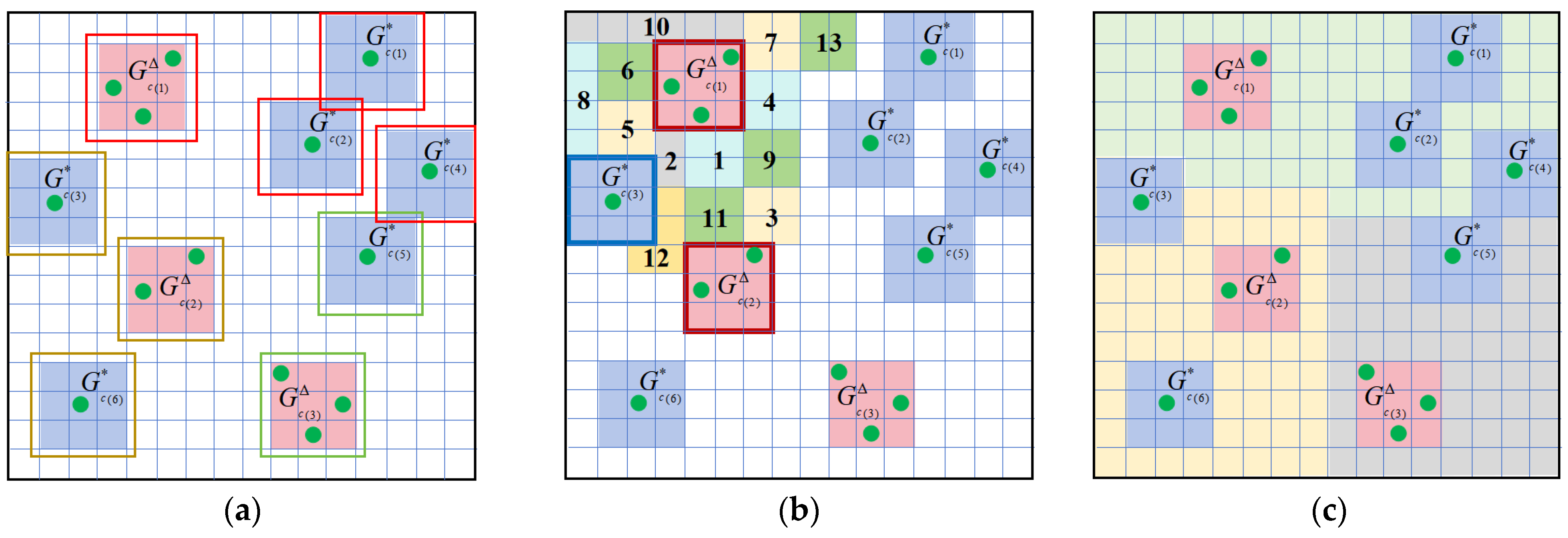
Determine the spatial positioning of cluster center cells $G_{c(i)}^{\mathrm{\Delta }}$ and cluster member cells $G_{c(i)}^{*}$ in matrix $M_{C(i)}$, as shown in Figure 5a. The red cell is cluster center cell $G_{c(i)}^{\mathrm{\Delta }}$, the blue cell is cluster member cell $G_{c(i)}^{*}$, and the red, brown, and green solid lines represent the regions and cells of the three clusters $C_{(i)}$.

(2)

Based on the constructed ISG spatial model and the $h^{*}$ number of neighborhood topological cells $G_{t(i)}$ in the second row of the cluster initial Open List, take the cluster center cells $G_{c(i)}^{\mathrm{\Delta }}$ and cluster member cells $G_{c(i)}^{*}$ as the centers, and search for the neighborhood topological cells $G_{t(i)}$. Figure 5b shows an example of generating topological cells $G_{t(i)}$ around $G_{c(1)}^{\mathrm{\Delta }}$, $G_{c(2)}^{\mathrm{\Delta }}$ and $G_{c(3)}^{\mathrm{\Delta }}$. The encoded $2\times 2$ area regions with different colors in the figure are the topological cells $G_{t(i)}$.

(3)

Include the topological cells $G_{t(i)}$ into the neighborhood clusters $C_{(i)}$ to form the tourism sub-regions, as shown in Figure 5c. The green, yellow, and gray areas in the figure are all the tourism sub-regions generated by the topological process of the cell clusters.

3.2. Tourism Hotel Recommendation Model Based on IDFST Optimal Route Algorithm

Tourism sub-regions divide the entire city region $S_c$ into the lower-dimensional spatial ranges, which can improve the efficiency of the recommendation algorithm and reduce the tourism transportation costs for tourists. When scenic spots within a certain tourism sub-region can meet tourists’ interests, recommending scenic spots within the sub-region can reduce transportation costs for tourists to travel between the scenic spots while meeting their interests and demands. In order to further improve tourism efficiency and reduce the cost of tourism transportation routes, it is also necessary to study the spatial relationship between hotels and scenic spots in sub-region and tour route costs starting from the hotels, then recommend hotels with the optimal spatial location for tourists [22,23,24,25]. To address this issue, we construct a tourism hotel recommendation model based on the IDFST optimal route algorithm, which includes three sub-models: the first one is a scenic spot recommendation model based on Attribute Closeness. Firstly, it explores tourists’ interests and recommends the most suitable scenic spots that match their interests based on the attributes of scenic spots in the sub-region, in order to ensure their satisfactions. The second one is a tourism sub-interval optimal route algorithm based on IDFST. It takes the candidate hotels and the recommended scenic spots within the sub-region as route nodes in the space, then $w$ number of feasible routes are formed between any two nodes. Tourist ferrying between two nodes will generate transportation costs, which is the key factor in generating tour route costs. The third one is a tourism hotel recommendation model based on the optimal route decision forest algorithm. Starting from each candidate hotel and taking the recommended scenic spots as route nodes, a decision forest is constructed to search for the route with the lowest transportation cost, and then it recommends the optimal hotel for tourists.

The theoretical and innovative analysis of the three models are as follows:

(1)

Scenic spot recommendation model based on attribute closeness. We collect tourists’ interests based on their current needs and interests as important data for recommending scenic spots within tourism sub-regions. It is a personalized scenic spot recommendation model based on tourists’ interests, with higher accuracy in matching tourists’ interests.

(2)

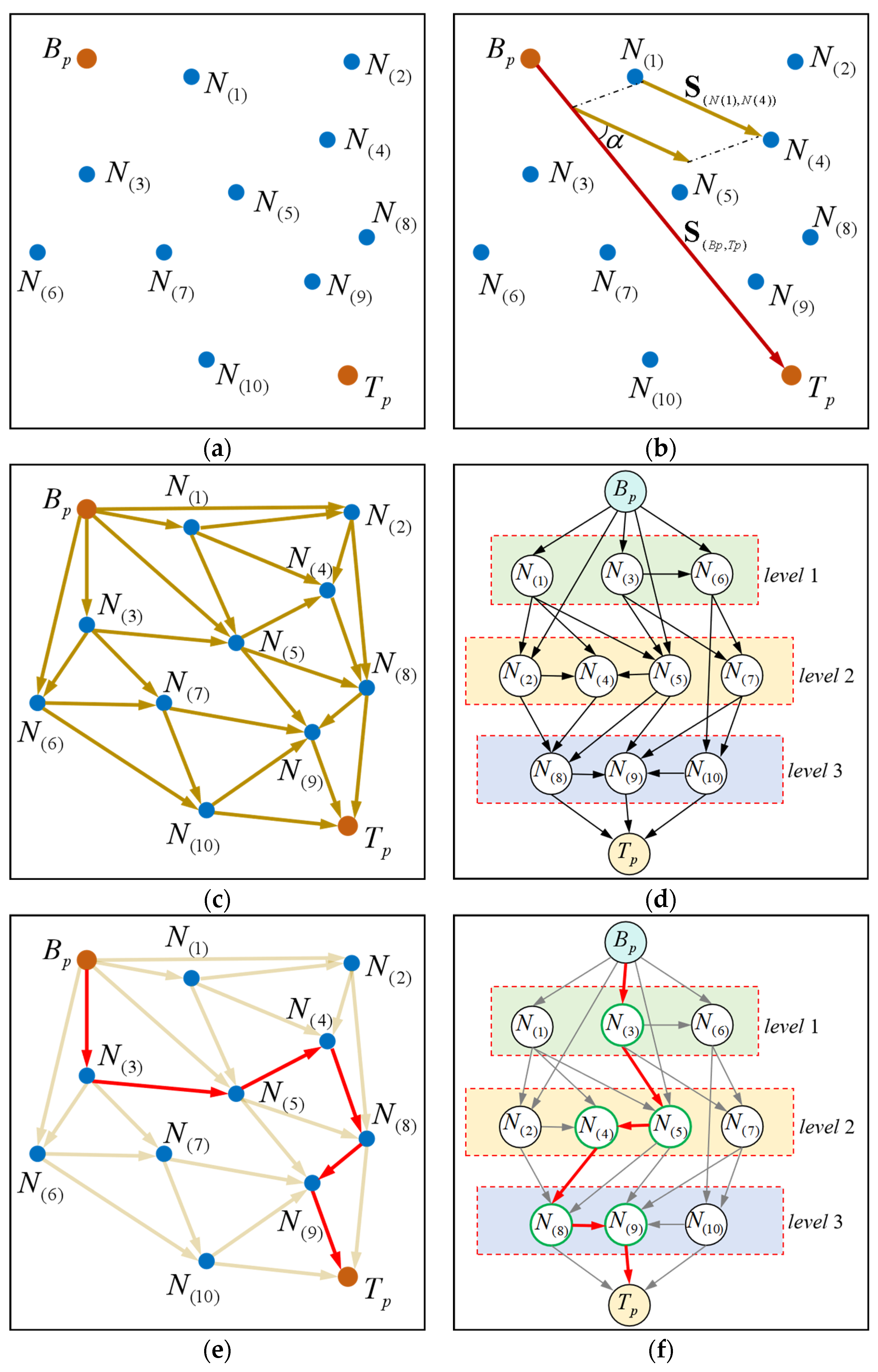
Tourism sub-interval optimal route algorithm based on IDFST. The constructed IDFST algorithm can output the global optimal route for each travel sub-interval, achieving optimization of the DFST algorithm. The traditional DFST algorithm integrates the idea of backtracking paths, which requires searching for the backtracking path of the current node and incorporating it into the search scope of the global path, resulting in a large computational cost. The constructed IDFST algorithm combines the actual urban geospatial conditions and the actual direction of tour routes, using an azimuth to remove the backtracking path of the current point, reducing the computational complexity.

(3)

Tourism hotel recommendation model based on the optimal route decision forest algorithm. The constructed hotel recommendation algorithm combines the idea of global optimal cost of tour routes. It starts from hotels within the tourism sub-region and uses the recommended scenic spots as route nodes to search for the global optimal tour routes and construct decision trees. Then, it constructs a decision forest from multiple hotels and searches for the optimal hotel from the decision forest. From the perspective of algorithm logic analysis, it is certain that the global optimal hotel with the lowest cost of tour route can be searched, reducing the travel cost of tourists to the lowest level.

3.2.1. Scenic Spot Recommendation Model Based on Attribute Closeness

We conduct the attribute mining on scenic spots within a tourism sub-region, and use attribute labels as interest items for tourists to choose from. By quantifying the attribute labels of scenic spots and interest items of tourists, we establish the closeness relationship model between the two, and it recommends scenic spots within the sub-region for tourists.

Definition 12.

Scenic spot attribute label  $A_{(i)}$ and tourist interest label  $I_{(i)}$. On the tourism server, describe the attributes of scenic spots in the urban region  $S_c$, establish several attribute labels  $A_{(i)}$  to quantify the tourism functions and service attributes of the scenic spots, including  $A_{(i)}$: {$A_{(1)}$: the duration of the visit;  $A_{(2)}$: the cost of the visit;  $A_{(3)}$: the star rating;  $A_{(4)}$: the popularity}. Normalize the labels  $A_{(i)}$  to obtain the quantitative labels that describe the attributes of scenic spots. At the tourist terminal, provide corresponding labels  $I_{(i)}$  for the tourists to evaluate and score, including  $I_{(i)}$: {$I_{(1)}$: the duration of the visit;  $I_{(2)}$: the cost of the visit;  $I_{(3)}$: the star rating;  $I_{(4)}$: the popularity}. Each label is set to 1–10 points, and after the tourists score each label, the system normalizes the scores to obtain the quantitative values of the tourists’ interests.

Definition 13.

Scenic spot recommendation objective function  $f(A_{(i)},I_{(i)})$. By constructing the closeness model between the attributes of scenic spots and tourists’ interests, we recommend the most suitable scenic spots that match tourists’ interests. There is a strong correlation between the attribute labels of scenic spots and the interest labels of tourists. We establish the scenic spot recommendation objective function based on the Euclidean distance model, as shown in Formula (5);  $\delta$  is the normalization factor.

$$f(A_{(i)},I_{(i)})=\delta \times {\left[{\displaystyle \sum _{i=1}^{\max i}{\left(A_{(i)}-I_{(i)}\right)}^2}\right]}^{-{\displaystyle \frac{1}{2}}}$$

(5)

Here is the explanation of the objective function for recommending scenic spots. Firstly, in order to match tourists’ interests with the attributes of scenic spots, we design tourist interest labels based on the attribute labels of scenic spots. We agree that the two have the same dimension and numerical distribution interval, and the quantified value of each label is distributed within the (0,1) interval to maintain consistency in the calculation dimension. Secondly, when the labels are determined, the attributes of scenic spots can be determined, and they are fixed numerical values used to express the unique features of scenic spots. The quantification process of tourists’ interest labels varies with changes in their interests and the labels are uncertain values. Each tourist has personalized interests, and based on their own needs and interests, they rate interest labels to obtain quantitative values that describe their interests. The higher the scores are, the higher the tourists’ needs and interests in the labels will be, while the lower the scores are, the lower the tourists’ needs and interests in the labels will be. Therefore, the designed interest labels can express tourists’ preferences. Thirdly, the constructed objective function here is not based on the interest data of historical tourists, nor is it based on the evaluation and preference data of historical tourists. Instead, it is based on the instantaneous interests and choices of the current tourists, expressing the tourists’ interests in scenic spots during a single evaluation. Therefore, it does not involve mining historical data and is not applicable to the empirical data and the historical feedback data.

3.2.2. Tourism Sub-Interval Optimal Route Algorithm Based on IDFST

In graph algorithms, the depth first search algorithm (DFSA) is an algorithm that searches in-depth direction from the starting point to the endpoint to obtain feasible routes. It can ensure the search for a route from the starting point to the endpoint, but the cost of the route may be an approximate optimal solution [26,27,28,29]. To build the optimal route and cost model between hotels and scenic spots, we construct an improved depth first search tree algorithm (IDFST) to search for the optimal routes in sub-intervals between hotels and scenic spots, in order to construct the route with the lowest transportation cost between two points. To improve algorithm efficiency, enhance algorithm performance, and ensure that the optimal solution in the sub-interval could be found, we make improvements to the DFSA in the following aspects.

(1)

Optimize the tree structure of the sub-interval, with the middle nodes of the tree set as the road nodes, the root node set as the starting point of the sub-interval, and the highest level node uniformly set as the endpoint of the sub-interval.

(2)

Due to the non-repetition of the tour routes, the routes that have been visited are not repeated and there is no need to turn back. We set the spatial direction line to determine the direction of the tourist movement, so we remove the backtracking path in the tree structure and only keep the forward search path.

(3)

To avoid the negative impact of backtracking on the optimal solution, we collect all nodes and roads within a sub-interval, covering all levels of roads within the urban area. Under the condition of consistent urban scale and distance dimension, including backtracking paths will inevitably increase the cost of the current route, making the route that could have been the optimal solution become the sub-optimal solution. In addition, the backtracking path may increase the cost for a certain route A, but it may be a forward and reasonable path for another route B. Therefore, when route B appears as a candidate route for the optimal solution in the maximum heap, it contains the backtracking path. From this perspective, the deleted backtracking path is the reverse and cost-increasing path, rather than the path itself, ensuring the exhaustiveness and completeness of the route search within the sub-interval, enabling the algorithm to output the optimal solution. Meanwhile, due to the removal of the reverse backtracking path search, the time complexity of the constructed IDFST algorithm is superior to the traditional algorithm.

(4)

To ensure that the optimal solution in the sub-interval could be found, the algorithm searches for all the feasible routes and their costs, and stores the costs of all feasible routes in the maximum heap. Thus, it can cover all possible solutions and keep the exhaustiveness and completeness of the algorithm.

Definition 14.

Tourism sub-interval  $S_{I(i)}$, sub-interval starting point $B_p$, sub-interval ending point $T_p$, sub-interval node $N_{(i)}$. The movement interval generated by tourists’ ferrying between hotels and scenic spots by certain transportation methods within a tourism sub-region is defined as tourism sub-interval $S_{I(i)}$. The starting point of the sub-interval is a hotel or scenic spot, defined as sub-interval starting point $B_p$; the ending point of the sub-interval is also a hotel or scenic spot, defined as sub-interval ending point $T_p$; the road nodes that tourists pass through for ferrying within the sub-interval are defined as sub-interval node $N_{(i)}$. Figure 6a shows the examples of starting point $B_p$, ending point $T_p$, and nodes $N_{(i)}$ within a sub-interval $S_{I(i)}$.

Definition 15.

Sub-interval direction vector  $S_{(Bp,Tp)}$, sub-interval node direction vector $S_{(N(i),N(j))}$, node direction angle $\alpha$. The vector from the starting point $B_p$ to the endpoint $T_p$ within a sub-interval $S_{I(i)}$ is defined as sub-interval direction vector $S_{(Bp,Tp)}$. For any adjacent node $\forall N_{(i)}$ and $\forall N_{(j)}$, the vector from node $N_{(i)}$ to node $N_{(j)}$ is defined as sub-interval node direction vector $S_{(N(i),N(j))}$. The angle between vector $S_{(Bp,Tp)}$ and $S_{(N(i),N(j))}$ is defined as node direction angle $\alpha$. Figure 6b shows the examples of the vector $S_{(Bp,Tp)}$, vector $S_{(N(i),N(j))}$, and angle $\alpha$ between $S_{(Bp,Tp)}$ and $S_{(N(1),N(4))}$. For the definition, vectors and angle $\alpha$ satisfy the following conditions:

(1) 

When  $0<\alpha \le {\displaystyle \frac{\pi }{2}}$, the vector  $S_{(N(i),N(j))}$  is the search edge, preserved;

(2) 

When  ${\displaystyle \frac{\pi }{2}}<\alpha \le \pi$, the vector  $S_{(N(i),N(j))}$  is a backtracking edge, delete.

Definition 16.

Depth first search tree  $D_{Tre{e}_{(i)}}$. For a tourism sub-interval  $S_{I(i)}$, we establish a tree structure for the depth first search, with the starting point  $B_p$, ending point  $T_p$, and nodes  $N_{(i)}$  of the sub-interval  $S_{I(i)}$  as key nodes for constructing the search tree, and define the tree as a depth first search tree  $D_{Tre{e}_{(i)}}$. Its storage structure meets the following conditions:

(1) 

Delete the backtracking edges between tree nodes;

(2) 

The root node  $t_{(1,1)}$  of the tree stores the starting point  $B_p$, the middle node  $t_{(x,y)}$  stores the road node  $N_{(i)}$, and the highest level node  $t_{(\max x,y)}$  stores the endpoint  $T_p$;

(3) 

The search direction of the tree is from the root node  $t_{(1,1)}$  along the middle node  $t_{(x,y)}$  to the highest level node  $t_{(\max x,y)}$;

(4) 

When the layer numbers  $x$  of nodes are identical, the search edge can be established between different nodes  $t_{(x,y)}$  and  $t_{(x,z)}$,  $y\ne z$;

(5) 

When the layer number satisfies  $x>y$, any node  $\forall t_{(y,*)}$  in the layer  $y$  can establish a search edge to any node  $\forall t_{(x,*)}$  in the layer  $x$, but  $\forall t_{(x,*)}$  cannot establish a search edge to node  $\forall t_{(y,*)}$;

(6) 

There is no independent or disconnected node.

Definition 17.

Node path  $P_{(i)}$, path cost  $C_{P(i)}$, sub-interval feasible route  $Ro{u}_{(i)}$, sub-interval feasible route cost  $C_{Rou(i)}$, sub-interval feasible route cost index  ${\delta }_{Rou(i)}$. Two adjacent nodes in tree  $D_{Tre{e}_{(i)}}$  are connected by a search edge, which is defined as node path  $P_{(i)}$. In the urban geographic space, the minimum distance traveled by tourists on the node path  $P_{(i)}$  when they move from one node to an adjacent node is defined as path cost  $C_{P(i)}$. Within a sub-interval, the process of tourists starting from the starting point  $B_p$, passing through several nodes  $N_{(i)}$, and finally reaching the endpoint  $T_p$  forms a complete route, which is defined as the sub-interval feasible route  $Ro{u}_{(i)}$. According to the definition, the route  $Ro{u}_{(i)}$  is composed of multiple paths  $P_{(i)}$, and the total distance of the entire route formed by iterating the costs  $C_{P(i)}$  of multiple paths  $P_{(i)}$  is defined as sub-interval feasible route cost  $C_{Rou(i)}$, as shown in Formula (6). To represent the optimal sub-interval route through the maximum heap, we define the sub-interval feasible route cost index  ${\delta }_{Rou(i)}$, as shown in Formula (7).

$$C_{Rou(i)}={\displaystyle \sum _{i=1}^{\max i}{C}_{P(i)}}$$

(6)

$${\delta }_{Rou(i)}={\displaystyle \frac{1}{{\displaystyle \sum _{i=1}^{\max i}{C}_{P(i)}}}}$$

(7)

According to the geospatial relationships, each model in Definition 16 must meet the following conditions:

(1)

There is no closed interval or broken edge in $Ro{u}_{(i)}$, it must be a complete route;

(2)

When any path $\forall P_{(i)}$ changes, the route $Ro{u}_{(i)}$ immediately changes, resulting in a new route;

(3)

The included nodes $N(i)$ of $Ro{u}_{(i)}$ are the subset of all nodes within the sub-interval.

Definition 18.

Sub-interval route decision heap  $H_{Rou(i)}$. According to the geospatial conditions of sub-intervals, decision tree structure  $D_{Tre{e}_{(i)}}$, and principle of route  $Ro{u}_{(i)}$, one decision tree  $D_{Tre{e}_{(i)}}$  corresponds to several feasible routes  $Ro{u}_{(i)}$. When the number of feasible route is  $k$, construct the maximum heap containing  $k$  number of nodes, and define this maximum heap as the sub-interval route decision heap  $H_{Rou(i)}$. The heap  $H_{Rou(i)}$  conforms to a complete binary tree storage structure, and the data storage logic meets the requirements of the maximum heap.

According to Definition 14 to Definition 18, we construct a tourism sub-interval optimal route algorithm based on IDFST.

Step 1: Build sub-interval $S_{I(i)}$ containing the starting point $B_p$, the ending point $T_p$, and the nodes $N_{(i)}$, and construct sub-interval direction vector $S_{(Bp,Tp)}$. Take any adjacent nodes $\forall N_{(i)}$ and $\forall N_{(j)}$, construct node direction vector $S_{(\forall N(i),\forall N(j))}$. Store the starting point $B_p$, the endpoint $T_p$, and the nodes $N_{(i)}$ in the Open List.

Step 2: Calculate angle $\alpha$ between $S_{(Bp,Tp)}$ and $\forall S_{(\forall N(i),\forall N(j))}$. Determine the value $\alpha$ and remove the backtracking edge. Retain paths $P_{(i)}$ that only include the search edges. The sub-interval directed weighted edge graph is composed of the starting point $B_p$, the ending point $T_p$, the nodes $N_{(i)}$, and the paths $P_{(i)}$, with the edge weights $C_{P(i)}$ as shown in Figure 6c.

Step 3: Output a depth first search tree $D_{Tre{e}_{(i)}}$ based on the directed weighted edge graph, as shown in Figure 6d, where the blue circle is the starting point $B_p$, the yellow circle is the endpoint $T_p$, the white circle is the node $N_{(i)}$, and the black arrow is the search edge corresponding to the path $P_{(i)}$. Search for the first feasible route $Ro{u}_{(1)}$.

(1)

Start from the point $B_p$, randomly find $N_{(3)}$ in the first layer to form a path $P_{(1)}$: $S_{(Bp,N(3))}$, corresponding to the cost $C_{P(1)}$. Delete $B_p$ and $N_{(3)}$ from the Open List, and store in the Closed List.

(2)

Start from $N_{(3)}$, randomly find $N_{(5)}$ in the second layer to form a path $P_{(2)}$: $S_{(N(3),N(5))}$, corresponding to the cost $C_{P(2)}$. Delete $N_{(5)}$ from the Open List, and store in the Closed List.

(3)

Start from $N_{(5)}$, randomly find $N_{(4)}$ in the second layer to form a path $P_{(3)}$: $S_{(N(5),N(4))}$, corresponding to the cost $C_{P(3)}$. Delete $N_{(4)}$ from the Open List, and store in the Closed List.

(4)

Start from $N_{(4)}$, randomly find $N_{(8)}$ in the third layer to form a path $P_{(4)}$: $S_{(N(4),N(8))}$, corresponding to the cost $C_{P(4)}$. Delete $N_{(8)}$ from the Open List, and store in the Closed List.

(5)

Start from $N_{(8)}$, randomly find $N_{(9)}$ in the third layer to form a path $P_{(5)}$: $S_{(N(8),N(9))}$, corresponding to the cost $C_{P(5)}$. Delete $N_{(9)}$ from the Open List, and store in the Closed List.

(6)

Start from $N_{(9)}$, find the ending point $T_p$, form a path $P_{(6)}$: $S_{(N(9),Tp)}$, corresponding to the cost $C_{P(6)}$. Delete $T_p$ from the Open List, and store in the Closed List. complete the search.

(7)

Output the $Ro{u}_{(1)}$:{$S_{(Bp,N(3))}$, $S_{(N(3),N(5))}$, $S_{(N(5),N(4))}$, $S_{(N(4),N(8))}$, $S_{(N(8),N(9))}$, $S_{(N(9),Tp)}$}, the route cost $C_{Rou(1)}$ is ${\displaystyle {\sum }_{i=1}^6{C}_{P(i)}}$, calculate the route cost index ${\delta }_{Rou(1)}$. The feasible route $Ro{u}_{(1)}$ consists of the red vector set in Figure 6e, as well as the green nodes and red search edges labeled in the depth first search tree $D_{Tre{e}_{(i)}}$ in Figure 6f.

Step 4: Search for other feasible routes $Ro{u}_{(i)}$ by the same method as Step 3, calculate the route cost $C_{Rou(i)}$ and index ${\delta }_{Rou(i)}$, and obtain a total number of $k$ routes and their corresponding costs. Build a decision heap $H_{Rou(i)}$ with a node count of $k$, initialize $H_{Rou(i)}=0$, and record the nodes as $h_{(x,y)}$.

(1)

Take No. 1 route $Ro{u}_{(1)}$ and No. 2 route $Ro{u}_{(2)}$ and determine:

(i)

If ${\delta }_{Rou(1)}<{\delta }_{Rou(2)}$, store $Ro{u}_{(1)}$ and $Ro{u}_{(2)}$ into $h_{(2,1)}$ and $h_{(1,1)}$;

(ii)

If ${\delta }_{Rou(1)}\ge {\delta }_{Rou(2)}$, store $Ro{u}_{(1)}$ and $Ro{u}_{(2)}$ into $h_{(1,1)}$ and $h_{(2,1)}$;

(2)

Take No. 3 route $Ro{u}_{(3)}$ and determine:

(i)

When ${\delta }_{Rou(1)}<{\delta }_{Rou(2)}$:

①

If ${\delta }_{Rou(3)}\le {\delta }_{Rou(1)}<{\delta }_{Rou(2)}$, store $Ro{u}_{(1)}$, $Ro{u}_{(2)}$ and $Ro{u}_{(3)}$ into $h_{(2,1)}$, $h_{(1,1)}$ and $h_{(2,2)}$;

②

If ${\delta }_{Rou(1)}<{\delta }_{Rou(3)}\le {\delta }_{Rou(2)}$, store $Ro{u}_{(1)}$, $Ro{u}_{(2)}$ and $Ro{u}_{(3)}$ into $h_{(2,2)}$, $h_{(1,1)}$ and $h_{(2,1)}$;

③

If ${\delta }_{Rou(1)}<{\delta }_{Rou(2)}<{\delta }_{Rou(3)}$, store $Ro{u}_{(1)}$, $Ro{u}_{(2)}$ and $Ro{u}_{(3)}$ into $h_{(2,2)}$, $h_{(2,1)}$ and $h_{(1,1)}$;

(ii)

When ${\delta }_{Rou(1)}\ge {\delta }_{Rou(2)}$:

①

If ${\delta }_{Rou(3)}>{\delta }_{Rou(1)}\ge {\delta }_{Rou(2)}$, store $Ro{u}_{(1)}$, $Ro{u}_{(2)}$ and $Ro{u}_{(3)}$ into $h_{(2,1)}$, $h_{(2,2)}$ and $h_{(1,1)}$;

②

If ${\delta }_{Rou(1)}\ge {\delta }_{Rou(3)}\ge {\delta }_{Rou(2)}$, store $Ro{u}_{(1)}$, $Ro{u}_{(2)}$ and $Ro{u}_{(3)}$ into $h_{(1,1)}$, $h_{(2,2)}$ and $h_{(2,1)}$;

③

If ${\delta }_{Rou(1)}\ge {\delta }_{Rou(2)}>{\delta }_{Rou(3)}$, store $Ro{u}_{(1)}$, $Ro{u}_{(2)}$ and $Ro{u}_{(3)}$ into $h_{(1,1)}$, $h_{(2,1)}$ and $h_{(2,2)}$;

(3)

Take the No. $i$ route $Ro{u}_{(i)}$, compare cost index ${\delta }_{Rou(1)}$ to ${\delta }_{Rou(i)}$, store ${\delta }_{Rou(1)}$ to ${\delta }_{Rou(i)}$ into the maximum heap $H_{Rou(i)}$ in line with the storage rule, and traverse $i~(0,k]$.

(4)

When the traversal $i=k$ is complete, the index ${\delta }_{Rou(1)}$ to ${\delta }_{Rou(i)}$ are stored, and output the full ranked heap $H_{Rou(i)}$.

Step 5: Take the root node $h_{(1,1)}$ of the current heap $H_{Rou(i)}$, where the corresponding route cost index ${\delta }_{Rou(i)}$ is the maximum value and the route cost $C_{Rou(i)}$ is the minimum value, thus it stores the optimal route $Ro{u}_{(i)}^{opt}$ within the sub-interval $S_{I(i)}$.

Step 6: Construct all the sub-intervals $S_{I(i)}$ within tourism sub-region, and output the optimal route $Ro{u}_{(i)}^{opt}$, route cost $C_{Rou(i)}$, and route index ${\delta }_{Rou(i)}$ corresponding to all sub-intervals according to the algorithm from Step 1 to Step 5.

3.2.3. Tourism Hotel Recommendation Model Based on the Optimal Route Decision Forest Algorithm

Within a tourism sub-region, when the number of the recommended scenic spots $T_{(i)}$ is $m$, the number of the candidate hotels $H_{(i)}$ for tourists is $n$, then a large number of tourism sub-regions $S_{I(i)}$ and types of tour routes can be constructed. There will be $C_{m+1}^{m+1}$ kinds of sub-intervals $S_{I(i)}$ between the $m$ number of scenic spots $T_{(i)}$ and any hotel $\forall H_{(i)}$. When any hotel $\forall H_{(i)}$ is used as the starting and the ending point of a tour route, and tourists visit the $m$ number of scenic spots $T_{(i)}$, then the tour route is composed of $m+1$ number of sub-intervals $S_{I(i)}$. By calculating the tour route costs with different hotels as the starting and ending points and the recommended scenic spots as route nodes, the tour route with the lowest transportation cost can be obtained, then the optimal hotel for tourists can be recommended.

Therefore, the principle of the constructed tourism hotel recommendation model based on the optimal route decision forest algorithm is as follows. Firstly, select one arbitrary hotel within the tourism sub-region, with the hotel as the starting and ending points, and the recommended scenic spots as route nodes. According to the different travel orders, several feasible tour routes can be output. Establish a decision tree to store the cost indexes of the output tour routes, and iterate the sub-intervals of each tour route separately to obtain the tour route cost and cost index. Based on the decision tree, a maximum heap is constructed, and the cost indexes of each tour route are stored in the heap according to the maximum heap algorithm, resulting in a visualized decision tree in the form of maximum heap. The root node of the decision tree corresponds to the optimal tour route and cost index stored under the hotel condition. In line with the same algorithm, construct a decision tree and a maximum heap for each hotel, so that the root node of each decision tree stores the optimal tour route and cost index under each hotel condition, and then forms a decision forest from all decision trees. Take the cost index stored at the root node of each decision tree, and use the maximum heap algorithm to store the optimal cost indexes of all hotels in the heap. After iteration, the hotel corresponding to the cost index stored at the root node of the current maximum heap is the global optimal hotel, and it is recommended to the tourist.

The decision tree constructed in this algorithm has a strict correspondence with the maximum heap. Firstly, the decision tree and the maximum heap have the identical structure, both storing data in the form of complete binary tree. In this algorithm, one decision tree corresponding to a hotel within the sub-region corresponds to one maximum heap, with the same number of decision tree nodes and maximum heap nodes, and the same tree structure and heap structure. Secondly, the function of the maximum heap is to store the route cost indexes during the algorithm execution, and to achieve the maximum heap storage by the heap sorting algorithm. The cost indexes are stored in the heap structure in the form of maximum heap in descending order. After the final formation of the maximum heap structure, the cost indexes of the nodes in the maximum heap are stored in the corresponding decision tree to complete the storage of the route cost indexes in the decision tree.

From the perspective of algorithm logic analysis, the constructed hotel recommendation algorithm is reasonable and feasible, and can be explained from the following three aspects.

Firstly, from the perspective of decision tree, heap structure, and algorithm logic. For a decision tree and its corresponding maximum heap, the maximum heap ranking of each tour route and cost index corresponding to the hotel is performed. The logic and time complexity analysis of the heap ranking algorithm are as follows:

(1)

The maximum heap is a complete binary tree, stored in array order. The complete binary tree height with $n$ number of nodes is $h=⌈{\log }_2(n+1)⌉$.

(2)

Build a heap. Traverse all parent nodes forward from the last non-leaf node, perform sinking adjustments one by one, with a time complexity of $O(n)$.

(3)

Loop sinking. The loop is executed by a total of times $n-1$, with two fixed steps each time: swapping the maximum value at the top of the heap with the current tail element, and grouping the tail element into an ordered region. Reduce the heap length by 1 and perform the sinking adjustment on the new heap top to restore the maximum heap. The total cost is $O(n\log n)$.

(4)

Merge the heap building time and the loop sinking time to obtain the overall complexity: $T(n)=O(n)+O(n\log n)$. The asymptotic complexity takes the high-order dominant term, and the final complexity is $O(n\log n)$.

Secondly, from the perspective of hotel recommendation and selection. After obtaining the $n$ number of maximum heaps corresponding to all hotels, transfer and store them to the corresponding $n$ number of decision trees. Take the optimal route cost index of each decision tree root node, and finally obtain the $n$ number of optimal route cost indexes for all hotels. Perform one more maximum heap sorting algorithm on the $n$ number of optimal route cost indexes of the hotels. Based on the above analysis and the same logic of the maximum heap sorting algorithm, its time complexity is still $O(n\log n)$.

Thirdly, from the perspective of algorithm efficiency. When the number $n$ of route nodes composed of hotels and scenic spots is very small ($n\le 100$), the algorithm’s computation speed under the time complexity $O(n\log n)$ is extremely fast, belonging to the microsecond level. Therefore, the constructed algorithm is of very high quality and can definitely output the global optimal solution at an extremely high speed, and can recommend the best hotels for tourists.

Definition 19.

Sub-region tour route  $T_{Rou(i)}$. In tourism sub-region, the arbitrary candidate hotel $\forall H_{(i)}$ is set as the starting point and the ending point, $m$ number of scenic spots $T_{(i)}$ are set as route nodes. Tourists visit the scenic spots in a certain sequence and it forms a complete route, and the route is defined as the sub-region tour route $T_{Rou(i)}$. When the order of sightseeing changes, the order of the sub-intervals $S_{I(i)}$ that make up the route $T_{Rou(i)}$ also change accordingly. The sub-intervals generated by the hotel $H_{(i)}$ and $m$ number of scenic spots $T_{(i)}$ have $C_{m+1}^{m+1}$ types, and the generated tour routes have $A_m^m$ types, then for the route $T_{Rou(i)}$, there are $0<i\le A_m^m$, $i,A_m^m\in Z^{+}$.

Definition 20.

Tour route cost  $C_{T\cdot Rou(i)}$, tour route cost index  ${\delta }_{T\cdot Rou(i)}$. The transportation cost incurred by the tourists on any route  $\forall T_{Rou(i)}$  is defined as the tour route cost  $C_{T\cdot Rou(i)}$, which is the cost generated by the iteration of the  $m+1$  number of sub-intervals  $S_{I(i)}$  on the route, as shown in Formula (8),  $C_{Rou(i)}$  is the sub-interval  $S_{I(i)}$  cost. To represent the optimal tour route through the maximum heap, we define the tour route cost index  ${\delta }_{T\cdot Rou(i)}$  as shown in Formula (9).

$$C_{T\cdot Rou(i)}={\displaystyle \sum _{i=1}^{m+1}{C}_{Rou(i)}}$$

(8)

$${\delta }_{T\cdot Rou(i)}={\displaystyle \frac{1}{{\displaystyle \sum _{i=1}^{m+1}{C}_{Rou(i)}}}}$$

(9)

Definition 21.

Tour route decision tree  $R_{Tree(i)}$, tour route decision forest  $F_{R\cdot Tree(i)}$. The types of tour routes composed of any hotel  $\forall H_{(i)}$  as the starting and ending point and  $m$  number of scenic spots  $T_{(i)}$  as the nodes are  $A_m^m$, then a complete binary tree with the  $A_m^m$  number of nodes is constructed to build the maximum heap, which is used to store the cost index  ${\delta }_{T\cdot Rou(i)}$  of  $A_m^m$  types of tour routes. This tree is defined as tour route decision tree  $R_{Tree(i)}$. According to the definition, one hotel  $H_{(i)}$  corresponds to one decision tree  $R_{Tre{e}_{(i)}}$. When there are  $n$  candidate hotels  $H_{(i)}$  within the tourism sub-region, then  $n$  number of decision trees  $R_{Tre{e}_{(i)}}$  will be generated in the entire sub-region, collectively forming the tour route decision forest  $F_{R\cdot Tree(i)}$. By searching for the global optimal solution in the forest  $F_{R\cdot Tree(i)}$, the optimal tour route  $T_{Rou(i)}^{opt}$  and the hotel  $H_{(i)}^{opt}$  within the tourism sub-region can be obtained.

Definition 22.

Optimal hotel recommendation decision heap  $D_{H(i)}$. Search for the optimal cost index ${\delta }_{T\cdot Rou(i)}$ for $n$ number of decision trees $R_{Tre{e}_{(i)}}$ in the forest $F_{R\cdot Tree(i)}$, resulting in a total of $n$ local optimal cost indices ${\delta }_{T\cdot Rou(i)}$. By establishing a maximum heap to store the $n$ number of local optimal cost indices ${\delta }_{T\cdot Rou(i)}$, the global optimal cost index ${\delta }_{T\cdot Rou(i)}^{opt}$ is obtained. The corresponding tour route is the global optimal tour route $T_{Rou(i)}^{opt}$, which has the lowest cost $C_{T\cdot Rou(i)}$ and the highest cost index ${\delta }_{T\cdot Rou(i)}$. The hotel corresponding to the global optimal tour route $T_{Rou(i)}^{opt}$ is the best recommended hotel $H_{(i)}^{opt}$.

According to Definition 19 to Definition 22, we construct a tourism hotel recommendation model based on the optimal route decision forest algorithm.

Step 1: Determine the $m$ number of scenic spots $T_{(i)}$ and $n$ number of candidate hotels $H_{(i)}$ within the tourism sub-region, as well as all the sub-intervals $S_{I(i)}$ composed of hotels and scenic spots, and output the optimal route $Ro{u}_{(i)}^{opt}$ and optimal route cost $C_{Rou(i)}^{opt}$ for each sub-interval.

Step 2: Initialize the tour route decision tree $R_{Tree(1)}=0$. Select the first hotel $H_{(1)}$ and determine the $C_{m+1}^2$ number of sub-intervals composed of hotel $H_{(1)}$ and $m$ number of scenic spots $T_{(i)}$. Search for tour routes $T_{Rou(i)}$ formed by the hotel $H_{(1)}$.

(1)

Search to determine the tour route $T_{Rou(1)}$. Iteratively calculate the route cost $C_{T\cdot Rou(1)}$ and output the route cost index ${\delta }_{T\cdot Rou(1)}$;

(2)

Search to determine the tour route $T_{Rou(2)}$. Iteratively calculate the route cost $C_{T\cdot Rou(2)}$ and output the route cost index ${\delta }_{T\cdot Rou(2)}$;

(3)

Compare ${\delta }_{T\cdot Rou(1)}$ and ${\delta }_{T\cdot Rou(2)}$:

(i)

If ${\delta }_{T\cdot Rou(1)}\ge {\delta }_{T\cdot Rou(2)}$, store ${\delta }_{T\cdot Rou(1)}$ and ${\delta }_{T\cdot Rou(2)}$ into nodes $h_{(1,1)}$ and $h_{(2,1)}$ in tree $R_{Tree(1)}$;

(ii)

If ${\delta }_{T\cdot Rou(1)}<{\delta }_{T\cdot Rou(2)}$, store ${\delta }_{T\cdot Rou(1)}$ and ${\delta }_{T\cdot Rou(2)}$ into nodes $h_{(1,1)}$ and $h_{(2,1)}$ in tree $R_{Tree(1)}$.

(4)

Search to determine the tour route $T_{Rou(3)}$. Iteratively calculate the route cost $C_{T\cdot Rou(3)}$ and output the route cost index ${\delta }_{T\cdot Rou(3)}$; Compare ${\delta }_{T\cdot Rou(1)}$, ${\delta }_{T\cdot Rou(2)}$ and ${\delta }_{T\cdot Rou(3)}$:

(i)

If ${\delta }_{T\cdot Rou(1)}\ge {\delta }_{T\cdot Rou(2)}$:

①

If ${\delta }_{T\cdot Rou(3)}\ge {\delta }_{T\cdot Rou(1)}\ge {\delta }_{T\cdot Rou(2)}$, store ${\delta }_{T\cdot Rou(1)}$, ${\delta }_{T\cdot Rou(2)}$ and ${\delta }_{T\cdot Rou(3)}$ into nodes $h_{(2,1)}$, $h_{(2,2)}$ and $h_{(1,1)}$ in tree $R_{Tree(1)}$;

②

If ${\delta }_{T\cdot Rou(1)}>{\delta }_{T\cdot Rou(3)}\ge {\delta }_{T\cdot Rou(2)}$, store ${\delta }_{T\cdot Rou(1)}$, ${\delta }_{T\cdot Rou(2)}$ and ${\delta }_{T\cdot Rou(3)}$ into nodes $h_{(1,1)}$, $h_{(2,2)}$ and $h_{(2,1)}$ in tree $R_{Tree(1)}$;

③

If ${\delta }_{T\cdot Rou(1)}\ge {\delta }_{T\cdot Rou(2)}>{\delta }_{T\cdot Rou(3)}$, store ${\delta }_{T\cdot Rou(1)}$, ${\delta }_{T\cdot Rou(2)}$ and ${\delta }_{T\cdot Rou(3)}$ into nodes $h_{(1,1)}$, $h_{(2,1)}$ and $h_{(2,2)}$ in tree $R_{Tree(1)}$;

(ii)

If ${\delta }_{T\cdot Rou(1)}<{\delta }_{T\cdot Rou(2)}$:

①

If ${\delta }_{T\cdot Rou(3)}\le {\delta }_{T\cdot Rou(1)}<{\delta }_{T\cdot Rou(2)}$, store ${\delta }_{T\cdot Rou(1)}$, ${\delta }_{T\cdot Rou(2)}$ and ${\delta }_{T\cdot Rou(3)}$ into nodes $h_{(2,1)}$, $h_{(1,1)}$ and $h_{(2,2)}$ in tree $R_{Tree(1)}$;

②

If ${\delta }_{T\cdot Rou(1)}<{\delta }_{T\cdot Rou(3)}<{\delta }_{T\cdot Rou(2)}$, store ${\delta }_{T\cdot Rou(1)}$, ${\delta }_{T\cdot Rou(2)}$ and ${\delta }_{T\cdot Rou(3)}$ into nodes $h_{(2,2)}$, $h_{(1,1)}$ and $h_{(2,1)}$ in tree $R_{Tree(1)}$;

③

If ${\delta }_{T\cdot Rou(1)}<{\delta }_{T\cdot Rou(2)}\le {\delta }_{T\cdot Rou(3)}$, store ${\delta }_{T\cdot Rou(1)}$, ${\delta }_{T\cdot Rou(2)}$ and ${\delta }_{T\cdot Rou(3)}$ into nodes $h_{(2,2)}$, $h_{(2,1)}$ and $h_{(1,1)}$ in tree $R_{Tree(1)}$.

(5)

Search to determine the tour route $T_{Rou(i)}$. Iteratively calculate the route cost $C_{T\cdot Rou(i)}$ and output the route cost index ${\delta }_{T\cdot Rou(i)}$; Compare ${\delta }_{T\cdot Rou(1)}$~${\delta }_{T\cdot Rou(i)}$ and store ${\delta }_{T\cdot Rou(1)}$~${\delta }_{T\cdot Rou(i)}$ into the previous $i$ nodes of tree $R_{Tree(1)}$ according to the maximum heap storage rule.

(6)

Traverse $i~(0,A_m^m]$, when the traversal $i=A_m^m$ is completed, cost index ${\delta }_{T\cdot Rou(1)}$ to ${\delta }_{T\cdot Rou(i)}$ are stored, and a full ranked tree $R_{Tree(1)}$ is output. The tour route $T_{Rou(i)}$ stored at the root node $h_{(1,1)}$ of the current tree $R_{Tree(1)}$ is the optimal tour route of the tree and also the local optimal tour route of the forest $F_{R\cdot Tree(i)}$, denoted as $T_{Rou(i)}^{lopt-1}$, and its cost index is denoted as ${\delta }_{T\cdot Rou(i)}^{lopt-1}$.

Step 3: Initialize the tour route decision tree $R_{Tree(2)}=0$. Select the second hotel $H_{(2)}$ and output the local optimal tour route $T_{Rou(i)}^{lopt-2}$ of the tree $R_{Tree(2)}$ by using the same algorithm as Step 2, with the cost index of ${\delta }_{T\cdot Rou(i)}^{lopt-2}$, which is the second local optimal tour route of the forest $F_{R\cdot Tree(i)}$.

Step 4: Compare ${\delta }_{T\cdot Rou(i)}^{lopt-1}$ and ${\delta }_{T\cdot Rou(i)}^{lopt-2}$:

(1)

If ${\delta }_{T\cdot Rou(i)}^{lopt-1}\ge {\delta }_{T\cdot Rou(i)}^{lopt-2}$, store ${\delta }_{T\cdot Rou(i)}^{lopt-1}$ and ${\delta }_{T\cdot Rou(i)}^{lopt-2}$ into nodes $h_{(1,1)}$ and $h_{(2,1)}$ in heap $D_{H(i)}$;

(2)

If ${\delta }_{T\cdot Rou(i)}^{lopt-1}<{\delta }_{T\cdot Rou(i)}^{lopt-2}$, store ${\delta }_{T\cdot Rou(i)}^{lopt-1}$ and ${\delta }_{T\cdot Rou(i)}^{lopt-2}$ into nodes $h_{(2,1)}$ and $h_{(1,1)}$ in heap $D_{H(i)}$;

Step 5: Initialize the tour route decision tree $R_{Tree(3)}=0$. Select the third hotel $H_{(3)}$ and output the local optimal tour route $T_{Rou(i)}^{lopt-3}$ of the tree $R_{Tree(3)}$ by using the same algorithm as Step 2, with the cost index of ${\delta }_{T\cdot Rou(i)}^{lopt-3}$, which is the third local optimal tour route of the forest $F_{R\cdot Tree(i)}$. Compare ${\delta }_{T\cdot Rou(i)}^{lopt-1}$, ${\delta }_{T\cdot Rou(i)}^{lopt-2}$ and ${\delta }_{T\cdot Rou(i)}^{lopt-3}$:

(1)

If ${\delta }_{T\cdot Rou(i)}^{lopt-1}\ge {\delta }_{T\cdot Rou(i)}^{lopt-2}$:

(i)

If ${\delta }_{T\cdot Rou(i)}^{lopt-3}\ge {\delta }_{T\cdot Rou(i)}^{lopt-1}\ge {\delta }_{T\cdot Rou(i)}^{lopt-2}$, store ${\delta }_{T\cdot Rou(i)}^{lopt-1}$, ${\delta }_{T\cdot Rou(i)}^{lopt-2}$ and ${\delta }_{T\cdot Rou(i)}^{lopt-3}$ into nodes $h_{(2,1)}$, $h_{(2,2)}$ and $h_{(1,1)}$ in heap $D_{H(i)}$;

(ii)

If ${\delta }_{T\cdot Rou(i)}^{lopt-1}>{\delta }_{T\cdot Rou(i)}^{lopt-3}\ge {\delta }_{T\cdot Rou(i)}^{lopt-2}$, store ${\delta }_{T\cdot Rou(i)}^{lopt-1}$, ${\delta }_{T\cdot Rou(i)}^{lopt-2}$ and ${\delta }_{T\cdot Rou(i)}^{lopt-3}$ into nodes $h_{(1,1)}$, $h_{(2,2)}$ and $h_{(2,1)}$ in heap $D_{H(i)}$;

(iii)

If ${\delta }_{T\cdot Rou(i)}^{lopt-1}\ge {\delta }_{T\cdot Rou(i)}^{lopt-2}>{\delta }_{T\cdot Rou(i)}^{lopt-3}$, store ${\delta }_{T\cdot Rou(i)}^{lopt-1}$, ${\delta }_{T\cdot Rou(i)}^{lopt-2}$ and ${\delta }_{T\cdot Rou(i)}^{lopt-3}$ into nodes $h_{(1,1)}$, $h_{(2,1)}$ and $h_{(2,2)}$ in heap $D_{H(i)}$;

(2)

If ${\delta }_{T\cdot Rou(i)}^{lopt-1}<{\delta }_{T\cdot Rou(i)}^{lopt-2}$:

(i)

If ${\delta }_{T\cdot Rou(i)}^{lopt-3}\le {\delta }_{T\cdot Rou(i)}^{lopt-1}<{\delta }_{T\cdot Rou(i)}^{lopt-2}$, store ${\delta }_{T\cdot Rou(i)}^{lopt-1}$, ${\delta }_{T\cdot Rou(i)}^{lopt-2}$ and ${\delta }_{T\cdot Rou(i)}^{lopt-3}$ into nodes $h_{(2,1)}$, $h_{(1,1)}$ and $h_{(2,2)}$ in heap $D_{H(i)}$;

(ii)

If ${\delta }_{T\cdot Rou(i)}^{lopt-1}<{\delta }_{T\cdot Rou(i)}^{lopt-3}<{\delta }_{T\cdot Rou(i)}^{lopt-2}$, store ${\delta }_{T\cdot Rou(i)}^{lopt-1}$, ${\delta }_{T\cdot Rou(i)}^{lopt-2}$ and ${\delta }_{T\cdot Rou(i)}^{lopt-3}$ into nodes $h_{(2,2)}$, $h_{(1,1)}$ and $h_{(2,1)}$ in heap $D_{H(i)}$;

(iii)

If ${\delta }_{T\cdot Rou(i)}^{lopt-1}<{\delta }_{T\cdot Rou(i)}^{lopt-2}\le {\delta }_{T\cdot Rou(i)}^{lopt-3}$, store ${\delta }_{T\cdot Rou(i)}^{lopt-1}$, ${\delta }_{T\cdot Rou(i)}^{lopt-2}$ and ${\delta }_{T\cdot Rou(i)}^{lopt-3}$ into nodes $h_{(2,2)}$, $h_{(2,1)}$ and $h_{(1,1)}$ in heap $D_{H(i)}$.

Step 6: Initialize the tour route decision tree $R_{Tree(i)}=0$. Select the No. $i$ hotel $H_{(i)}$ and output the local optimal tour route $T_{Rou(i)}^{lopt-i}$ of the tree $R_{Tree(i)}$ by using the same algorithm as Step 2, with the cost index of ${\delta }_{T\cdot Rou(i)}^{lopt-i}$, which is the No. $i$ local optimal tour route of the forest $F_{R\cdot Tree(i)}$. Compare ${\delta }_{T\cdot Rou(i)}^{lopt-1}$~${\delta }_{T\cdot Rou(i)}^{lopt-i}$ and store ${\delta }_{T\cdot Rou(i)}^{lopt-1}$~${\delta }_{T\cdot Rou(i)}^{lopt-i}$ into the previous $i$ nodes in $D_{H(i)}$ according to the maximum heap storage rule.

Step 7: Traverse $i~(0,n]$. When the traversal $i=n$ is complete, the cost index ${\delta }_{T\cdot Rou(i)}^{lopt-1}$ to ${\delta }_{T\cdot Rou(i)}^{lopt-n}$ are stored, and the full ranked heap $D_{H(i)}$ is output. The cost index ${\delta }_{T\cdot Rou(i)}^{lopt-i}$ of the route stored in the root node $h_{(1,1)}$ of the current heap $D_{H(i)}$ is the global maximum index of the forest $F_{R\cdot Tree(i)}$, corresponding to the global minimum tour route cost. The hotel on the route is the global optimal hotel within the tourism sub-region.

4. Experimental Results and Analysis

4.1. Experimental Methods

To verify the feasibility and advantages of the constructed algorithm, we design experiments to analyze the ISG spatial topological model, the ISTING-AGNES clustering algorithm, and the optimal hotel recommendation. We also design comparative experiments to compare the constructed algorithm with the conventional algorithms. The basic ideas of the experiments are as follows: Select Chengdu, the capital city of Sichuan Province, China, as the research scope, and the specific research space is the main urban area of Chengdu city. Select representative scenic spots and hotels in Chengdu city as the research objects. Determine the geospatial coordinates of the scenic spots and the hotels. Generate spatial cell units, spatial operation matrix, scenic spot growth cells, and neighborhood topological cells through the constructed ISG spatial topological model, and finally output the ISG spatial model containing different cells. Based on the ISG spatial model, by using the constructed ISTING-AGNES clustering algorithm, the experiments output the clusters centered around scenic spot growth cells, and then absorb the neighborhood topological cells around the clusters to establish the tourism sub-region model. Taking a tourism sub-region as the scope of further research, identify the candidate hotels and scenic spots within the sub-region, then recommend scenic spots by collecting the interest data of the sample tourist, and then output the hotel and route with the lowest tour route cost by the constructed hotel recommendation algorithm. To verify the advantages of the algorithm, we design two sets of comparative experiments. The first group uses the commonly used Centroid Positioning Algorithm (CPA) in site selection methods to determine the optimal hotel, while the second group uses the Greedy Mountain Climbing Algorithm (GMCA) and Greedy Breadth First Search Algorithm (GBFSA) commonly used in the route planning to design routes, and compares them with the constructed algorithm.

4.2. Data Collection

For the experimental objectives, we collect the following data:

(1)

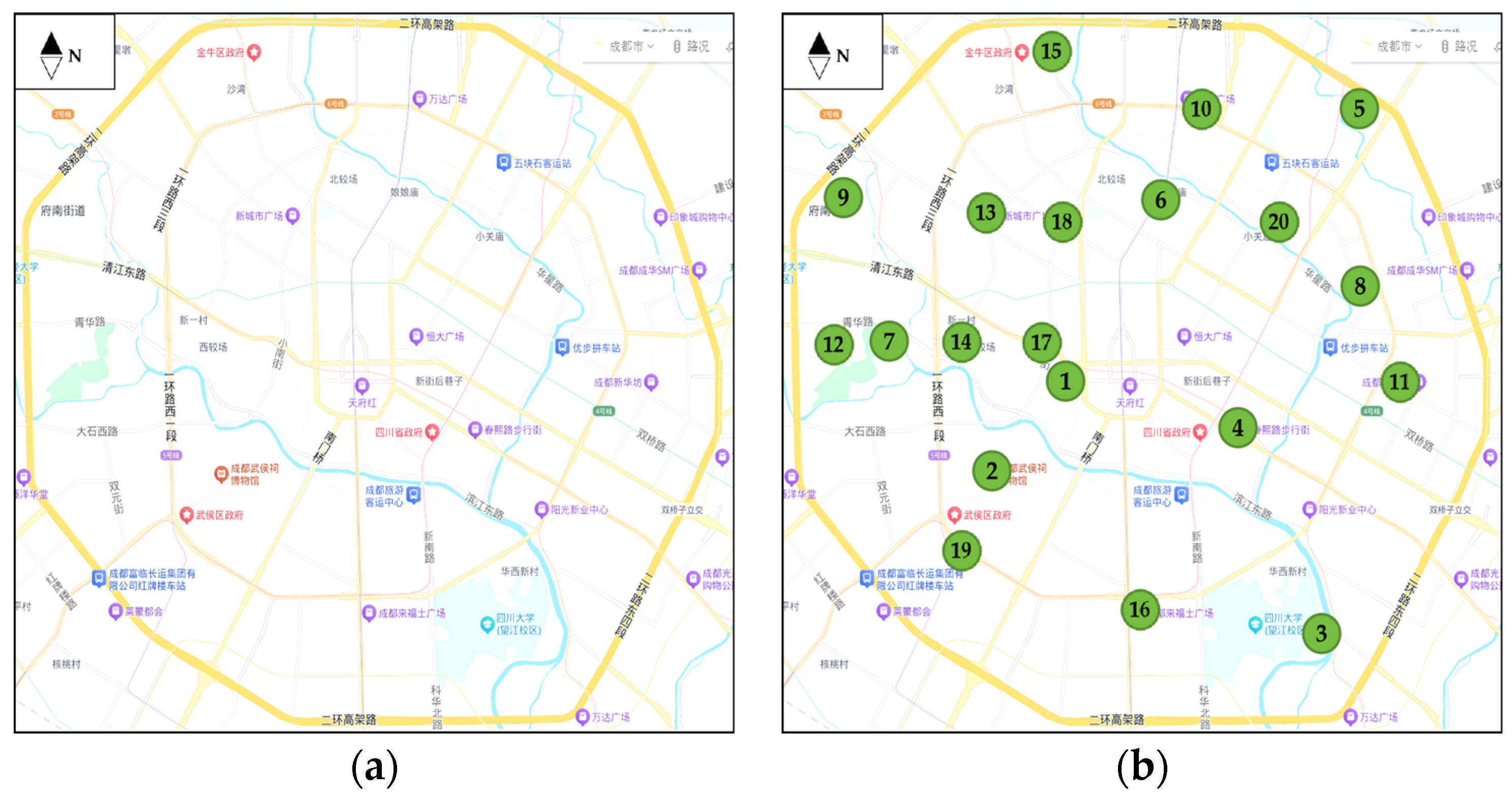
Based on the geospatial environment of Chengdu city, as well as the distribution status of hotels and scenic spots, the study area is divided by step size $a=1$ (unit: km), and a rectangular spatial range $S_c$ bounded by the Second Ring Road is collected. Figure 7a shows the selected research space range $S_c$. According to the modeling conditions, the dimension of region $S_c$ is obtained as $9\times 9$.

(2)

Collect 20 representative scenic spots (including commercial centers and other leisure destinations) within the Second Ring Road: $T_{(1)}$: People’s Park; $T_{(2)}$: Wuhou Temple; $T_{(3)}$: Wangjianglou Park; $T_{(4)}$: Chunxi Road; $T_{(5)}$: San Dong Gu Qiao Park; $T_{(6)}$: Wenshu Monastery; $T_{(7)}$: Sichuan Provincial Museum; $T_{(8)}$: Chenghua Park; $T_{(9)}$: Shi Ren Park; $T_{(10)}$: Jinniu Wanda Plaza; $T_{(11)}$: Xinhua Square; $T_{(12)}$: Du Fu Thatched Cottage; $T_{(13)}$: Yongling Museum; $T_{(14)}$: Qingyang Palace; $T_{(15)}$: Jiulidi Park; $T_{(16)}$: Raffles Square; $T_{(17)}$: Kuanzhai Alley; $T_{(18)}$: New City Square; $T_{(19)}$: Roman Holiday Plaza; $T_{(20)}$: Love Lane Cultural and Creative District. Figure 7b shows the distribution of scenic spots in region $S_c$.

Table 1. Representative scenic spots and their coordinates collected in the experiment.

	T(1)	T(2)	T(3)	T(4)	T(5)	T(6)	T(7)	T(8)	T(9)	T(10)
LT(i)	104.057	104.047	104.092	104.080	104.095	104.072	104.034	104.095	104.029	104.074
BT(i)	30.657	30.646	30.629	30.653	30.686	30.675	30.661	30.667	30.675	30.686
	T(11)	T(12)	T(13)	T(14)	T(15)	T(16)	T(17)	T(18)	T(19)	T(20)
LT(i)	104.105	104.028	104.047	104.042	104.056	104.068	104.053	104.057	104.042	104.085
BT(i)	30.656	30.660	30.674	30.660	30.691	30.631	30.663	30.673	30.637	30.674

shows the geospatial coordinates of scenic spots.

(3)

When tourism sub-regions are output in the experiment, select three representative hotels within each sub-region for candidate ones to recommend.

(4)

Select one sample tourist, and the interest labels provided by the tourist for scenic spots are $I_{(i)}$: {$I_{(1)}$: the duration of visit (2 h); $I_{(2)}$: the cost of visit (0 yuan); $I_{(3)}$: the star rating (4 A); $I_{(4)}$: the popularity (0.8 points)}. Collect and quantify attribute labels $A_{(i)}$ for the scenic spots.

(5)

Within the tourism sub-region, select candidate hotels and the recommended scenic spots as route nodes, collect the possible roads and road nodes between hotels and scenic spots within the sub-region, and also collect the travel distance between the road nodes. The collected travel distances must be the lowest level data that cannot be further divided.

4.3. Results and Analysis of the Scenic Spot ISG Spatial Model

Based on the designated region $S_c$ and scenic spots $T_{(i)}$ determined by the experiment, the urban area is divided into a spatial cell $C_{e(i,j)}$ array with $9\times 9$ dimension by step size $a=1$, and the tourist city spatial operation matrix ${\mathbf{M}}_{Sc}$ is constructed accordingly. Based on the cell $C_{e(i,j)}$ array and matrix ${\mathbf{M}}_{Sc}$, search and find the center cell, and then the constructed scenic spot growth cell algorithm is used to calculate the growth cells $G_{c(i)}$ and cell capacity $d_{(i)}$. On the basis of the growth cells in scenic spots, search for the neighborhood topological cells $G_{r(i)}$ within the search area $S_c$, and use the constructed cell topological algorithm to output the ISG spatial model corresponding to the area $S_c$. In the experiment, the dimension of the growth cell $G_{c(i)}$ of scenic spot is specified as $2\times 2$, and the dimension of the neighborhood topological cell $G_{t(i)}$ is specified as $1\times 1$. Figure 8a shows the calculated cell $C_{e(i,j)}$ array and matrix ${\mathbf{M}}_{Sc}$, with the brown area representing an example of the cell $C_{e(i,j)}$; Figure 8b shows the generated cell array containing scenic spots; Figure 8c shows the scenic spot growth cells $C_{t(i)}$ calculated by the algorithm, where the yellow area represents the scenic spot growth cells. To distinguish the boundaries, the different shades of yellow are used to represent the cells; Figure 8d shows the generated ISG space containing the neighborhood topological cells $G_{t(i)}$, where the $1\times 1$ blue area is an example of neighborhood topological cell, and the remaining white $1\times 1$ grids in the space are the neighborhood topological cells.

Table 2. The calculation results of the capacity of the scenic spot growth cells.

	Gc(1)	Gc(2)	Gc(3)	Gc(4)	Gc(5)	Gc(6)
Capacity d(i)	$d_{(1)}=1$	$d_{(2)}=2$	$d_{(3)}=2$	$d_{(4)}=1$	$d_{(5)}=2$	$d_{(6)}=2$
	Gc(7)	Gc(8)	Gc(9)	Gc(10)	Gc(11)	Gc(12)
Capacity d(i)	$d_{(7)}=4$	$d_{(8)}=1$	$d_{(9)}=2$	$d_{(10)}=1$	$d_{(11)}=1$	$d_{(12)}=1$

shows the calculation results of the capacity of the scenic spot growth cells $C_{e(i,j)}$.

Analyze the cell and ISG space output by the algorithm. In the result of Figure 8a, the urban area $S_c$ is divided into a spatial cell $C_{e(i,j)}$ array with dimension $9\times 9$ by step size $a=1$, which meets the requirements for constructing the scenic spot growth cells. Each cell unit is a grid with $1\times 1$ dimension covering a certain spatial range, providing the foundation for constructing the tourism sub-regions. In the result of Figure 8b, each scenic spot $T_{(i)}$ falls within one cell unit. The cell unit containing scenic spot is the center cell unit that constructs the scenic spot growth cell, while the cell unit without scenic spot is either absorbed into the growth cell or a neighborhood topological cell unit. In the result of Figure 8c, the algorithm generates a total of 12 scenic spot growth cells $G_{c(i)}$, and each cell has a different capacity, with a minimum capacity of $d_{(i)}=1$ and a maximum capacity of $d_{(i)}=4$. The cells with large capacity are the candidate center cells for generating clusters. In the result of Figure 8d, the algorithm generates a total of 31 neighborhood topological cells $G_{t(i)}$, represented by the white and blue grids in the figure with $1\times 1$ area. The neighborhood topological cells are distributed around scenic spot growth cells, which is the important factor in forming tourism sub-regions. From the number of scenic spot growth cells, the number of neighborhood topological cells, and the capacity of growth cells, it can be concluded that the constructed ISG algorithm can generate scenic spot growth cells and neighborhood topological cells with relatively balanced spatial distributions, and produce different cell capacities, indicating that the algorithm is reasonable and feasible.

4.4. Results and Analysis of the Clusters

According to the scenic spot growth cells $G_{c(i)}$ and the included scenic spots, the center positioning coordinates of each cell $G_{c(i)}$ are calculated as shown in

Table 3. Positioning coordinates of the scenic spots in cell and cell center.

Cell Gc(i)	The Contained Scenic Spot T(i)	LT(i)	BT(i)	LGc(i)	BGc(i)
Gc(1)	T(15)	104.056	30.691	104.056	30.691
Gc(2)	T(6)	104.072	30.675	104.073	30.681
	T(10)	104.074	30.686
Gc(3)	T(5)	104.095	30.686	104.090	30.680
	T(20)	104.085	30.674
Gc(4)	T(9)	104.029	30.675	104.029	30.675
Gc(5)	T(13)	104.047	30.674	104.052	30.674
	T(18)	104.057	30.673
Gc(6)	T(7)	104.034	30.661	104.031	30.661
	T(12)	104.028	30.66
G c(7)	T(1)	104.057	30.657	104.050	30.657
	T(2)	104.047	30.646
	T(14)	104.042	30.66
	T(17)	104.053	30.663
Gc(8)	T(4)	104.080	30.653	104.08	30.653
Gc(9)	T(8)	104.095	30.667	104.100	30.662
	T(11)	104.105	30.656
Gc(10)	T(19)	104.042	30.637	104.042	30.637
Gc(11)	T(16)	104.068	30.631	104.068	30.631
Gc(12)	T(3)	104.092	30.629	104.092	30.629

. Based on the result of the ISG space and the constructed ISTING-AGNES clustering algorithm, the calculated cluster center cells $G_{c(i)}^{\mathrm{\Delta }}$ in ISG space are as follows, with the number of clusters being $k=3$. The remaining cells $G_{c(i)}$ are cluster member cells $G_{c(i)}^{*}$.

(1)

The center cell $G_{c(i)}^{\mathrm{\Delta }}$ of cluster $C_{(1)}$ is $G_{c(2)}$.

(2)

The center cell $G_{c(i)}^{\mathrm{\Delta }}$ of cluster $C_{(2)}$ is $G_{c(7)}$.

(3)

The center cell $G_{c(i)}^{\mathrm{\Delta }}$ of cluster $C_{(3)}$ is $G_{c(9)}$.

Based on the latitude and longitude of each cell $G_{c(i)}$ output in Table 3, calculate the clustering objective function $f(G_{c(i)}^{*},G_{c(i)}^{\mathrm{\Delta }})$ between each cluster member cell $G_{c(i)}^{*}$ and cluster center cell $G_{c(i)}^{\mathrm{\Delta }}$, as shown in

Table 4. The clustering objective function values output by the algorithm.

	Gc(1)	Gc(3)	Gc(4)	Gc(5)	Gc(6)	Gc(8)	Gc(10)	Gc(11)	Gc(12)
Decision Tree	$Tre{e}_{(1)}$	$Tre{e}_{(2)}$	$Tre{e}_{(3)}$	$Tre{e}_{(4)}$	$Tre{e}_{(5)}$	$Tre{e}_{(6)}$	$Tre{e}_{(7)}$	$Tre{e}_{(8)}$	$Tre{e}_{(9)}$
Gc(2)	0.507	0.587	0.225	0.452	0.215	0.346	0.186	0.199	0.181
Gc(7)	0.290	0.217	0.362	0.584	0.515	0.330	0.464	0.316	0.198
Gc(9)	0.190	0.486	0.139	0.202	0.145	0.456	0.158	0.224	0.295

. Output the clustering decision tree $Tre{e}_{(u)}$ corresponding to each cluster member cell $G_{c(i)}^{*}$, as shown in Figure 9. The decision trees $Tre{e}_{(1)}$~$Tre{e}_{(9)}$ correspond to Figure 9a–i. Among them, the blue root nodes represent the center cell $G_{c(2)}$ as the maximum objective function value, the red root nodes represent the center cell $G_{c(7)}$ as the maximum objective function value, and the green root nodes represent the center cell $G_{c(9)}$ as the maximum objective function value.

Based on the calculation results of the clustering objective function values and the visualization results of the decision tree, we obtain clustering matrix $M_{C(i)}$, as well as the results of cell clusters $C_{(i)}$, cluster capacity $m_{(i)}$, cluster center cells $G_{c(i)}^{\mathrm{\Delta }}$, and cluster member cells $G_{c(i)}^{*}$, as shown in

Table 5. The experimental result of the output cluster matrix.

	Cluster Matrix ${\mathbf{M}}_{\mathit{C}(\mathit{i})}$		Cluster Capacity ${\mathit{m}}_{(\mathit{i})}$
Cluster	Cluster Center Cell ${\mathit{G}}_{\mathit{c}(\mathit{i})}^{\mathbf{\Delta }}$	Cluster Member Cell ${\mathit{G}}_{\mathit{c}(\mathit{i})}^{*}$
${\mathbf{C}}_{(1)}$	$G_{c(1)}^{\mathrm{\Delta }}$~$G_{c(2)}$	$G_{c(1)}$, $G_{c(3)}$	$m_{(1)}=3$
${\mathbf{C}}_{(2)}$	$G_{c(2)}^{\mathrm{\Delta }}$~$G_{c(7)}$	$G_{c(4)}$, $G_{c(5)}$, $G_{c(6)}$, $G_{c(10)}$, $G_{c(11)}$	$m_{(2)}=6$
${\mathbf{C}}_{(3)}$	$G_{c(3)}^{\mathrm{\Delta }}$~$G_{c(9)}$	$G_{c(8)}$, $G_{c(12)}$	$m_{(3)}=3$

. The left part of Table 5 represents the clustering matrix $M_{C(i)}$, and the right part represents the cluster capacity $m_{(i)}$. Based on the clustering results, using the constructed tourism sub-region model based on the cellular clusters $C_{(i)}$, each cluster absorbs the neighborhood topological cells $G_{t(i)}$ to form three tourism sub-regions.

Figure 10 shows the cell clusters $C_{(i)}$ and the tourism sub-regions generated by the clustering algorithm based on the constructed ISG spatial model. Figure 10a shows the calculated results of the cluster center cells $G_{c(i)}^{\mathrm{\Delta }}$ and the cluster member cells $G_{c(i)}^{*}$, with the brown area representing three cluster center cells $G_{c(i)}^{\mathrm{\Delta }}$ and the yellow area representing nine cluster member cells $G_{c(i)}^{*}$. Figure 10b shows the three cell clusters $C_{(i)}$ calculated by the clustering algorithm. The red dashed area represents the cluster $C_{(1)}$, the green dashed area represents the cluster $C_{(2)}$, and the blue dashed area represents the cluster $C_{(3)}$. Figure 10c shows the three tourism sub-regions output by the tourism sub-region algorithm. The red dashed area is the first tourism sub-region, the green dashed area is the second tourism sub-region, and the blue dashed area is the third tourism sub-region. Figure 10d shows the scope and the distribution of the tourism sub-regions including the urban blocks in the region $S_c$.

The following conclusions can be drawn from analyzing Table 3, Table 4 and Table 5 and Figure 9 and Figure 10:

(1)

In Table 3, the calculated center points and positioning coordinates of cells are different. When the number of scenic spot in a cell is 1, the positioning point of the cell is the scenic spot. When the number of scenic spots in a cell is greater than 1, the positioning point of the cell is the centroid of the scenic spots. As the goal of the clustering is to achieve the spatial gathering of scenic spots in the urban area $S_c$, the cellular localization algorithm uses the coordinates of scenic spots in the cell as the calculation standard, so that the calculation results of the clustering objective function are also based on the coordinates of scenic spots, and the clustering results are accurate and reasonable.

(2)

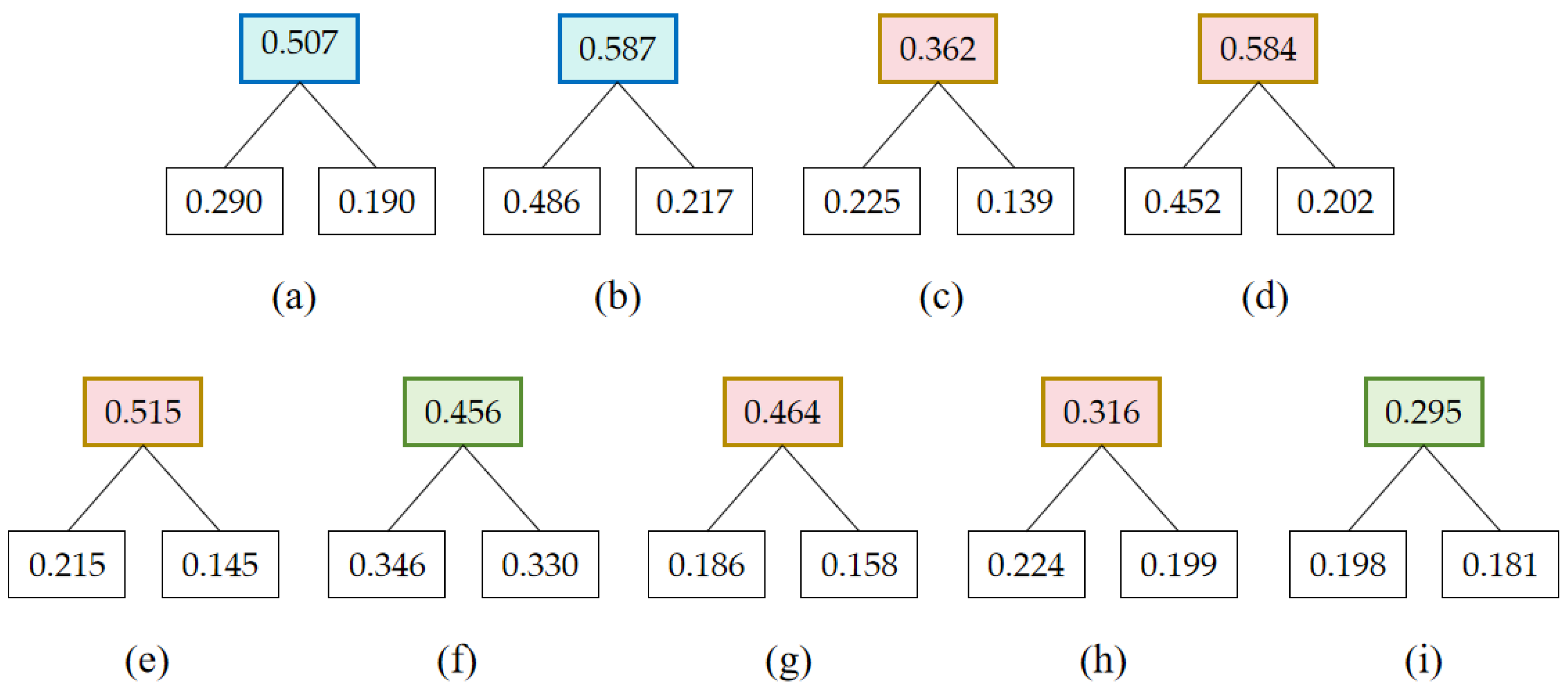
In Table 4, there are significant differences in the calculated clustering objective function values. For the same cluster center cell, the clustering objective function values generated by each cluster member cell show a fluctuating trend. The smaller the objective function value is, the more the cluster member cell deviation from the center cell will be, and vice versa, the closer it is to the center cell. For the same cluster member cell, the clustering objective function values generated by each cluster center cell vary greatly. The cluster center cell corresponding to the maximum objective function value is the cluster where the member cell is located.

(3)

Figure 9 shows the generated clustering decision trees based on the clustering algorithm from the results in Table 4. The number of the nodes in each decision tree is equal to the number of the center cells, and the cluster center cell corresponding to the root node is the cluster where the cluster member cell is located. Different colored root nodes represent the different clusters, with two blue root nodes, five red root nodes, and two green root nodes. This indicates that the distribution of cluster centers is relatively balanced compared to the entire decision tree, and there is no significant difference, demonstrating that the constructed clustering algorithm has spatial rationality. The number of red root nodes is relatively large, corresponding to the largest number of member cells in the cluster, while the other two root nodes correspond to relatively fewer member cells in the cluster.

(4)

In Table 5, the clustering algorithm outputs a cluster matrix with a reasonable storage structure. Each row in the matrix corresponds to one cluster, in which the cluster $C_{(1)}$ result is {$G_{c(2)}$| $G_{c(1)}$, $G_{c(3)}$}, the center cell of the cluster is $G_{c(2)}$, and the capacity is $m_{(1)}=3$; the cluster result $C_{(2)}$ is {$G_{c(7)}$| $G_{c(4)}$, $G_{c(5)}$, $G_{c(6)}$, $G_{c(10)}$, $G_{c(11)}$}, the center cell of the cluster is $G_{c(7)}$, and the capacity is $m_{(2)}=6$; the cluster $C_{(3)}$ result is {$G_{c(9)}$| $G_{c(8)}$, $G_{c(12)}$}, the center cell of the cluster is $G_{c(9)}$, and the capacity is $m_{(3)}=3$. From the results, it can be concluded that the constructed clustering algorithm can generate clusters with a relatively balanced number of cell members, and there is no significant difference in cluster capacity, indicating that the clustering effect of the clustering algorithm is fine.

(5)

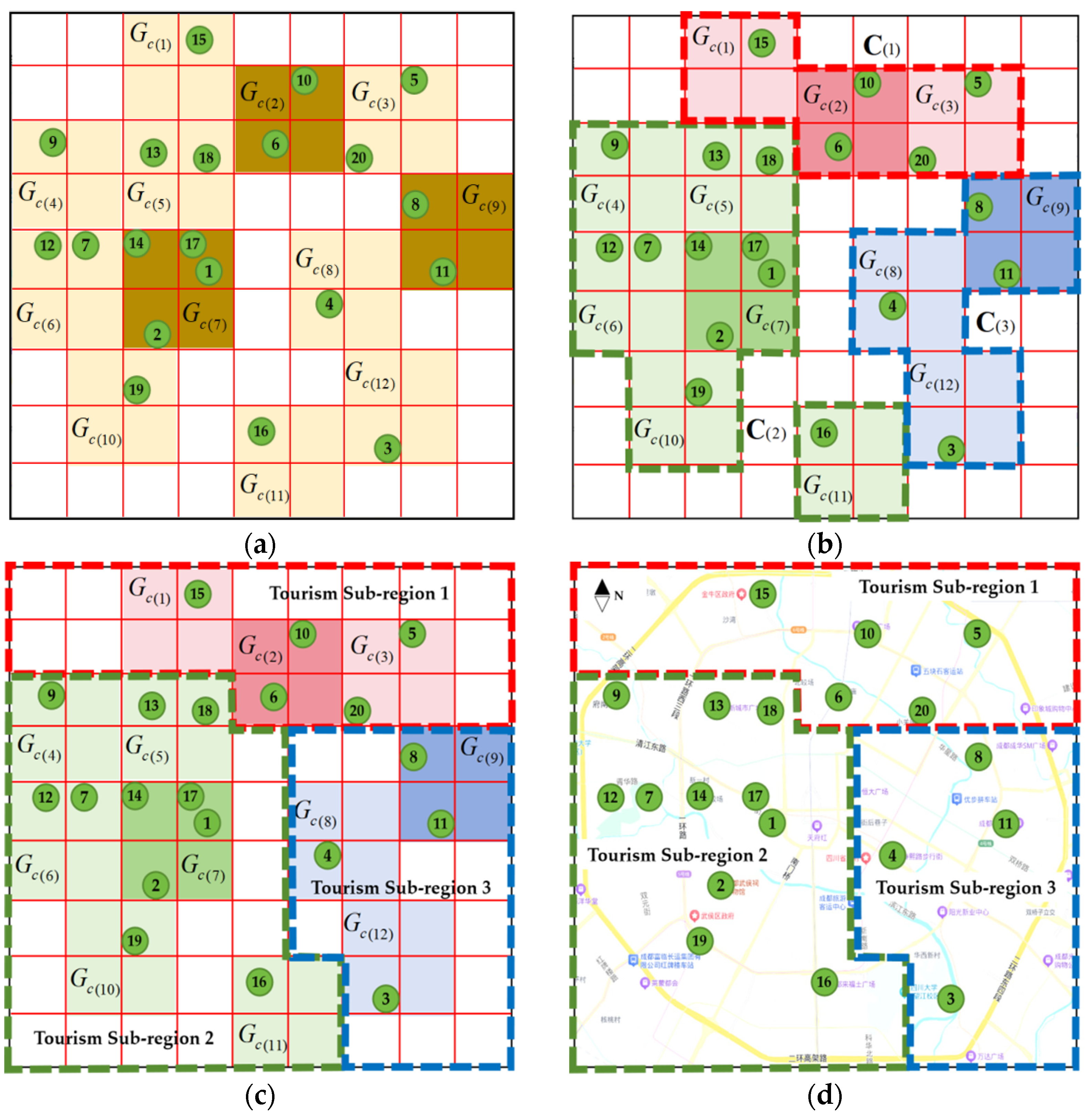
In Figure 10a, the distribution of cluster center cells in urban area $S_c$ is relatively discrete and balanced, and the distribution of cluster member cells is also relatively balanced, indicating that the clustering algorithm’s searching for cluster centers is logically reasonable and produces the high-quality cluster centers. The three clusters generated in Figure 10b contain different member cells, and the positions, ranges, and areas of the coverage areas are all different, indicating that the clustering algorithm can generate cluster spatial ranges with reasonable discrepancies, which conforms to the distribution law of relatively discrete and gathered scenic spots within a certain range in a city. The algorithm is reasonable. In Figure 10c,d, three clusters absorb neighborhood topological cells, and the number and capacity of each cluster’s absorption are balanced, resulting in three tourism sub-regions with relatively balanced areas, different location distributions, covering cluster cells, and a certain number of scenic spots. The first tourism sub-region contains 5 scenic spots, the second tourism sub-region contains 11 scenic spots, and the third tourism sub-region contains 4 scenic spots. The number of scenic spots in each tourism sub-region is relatively balanced with reasonable discrepancies, indicating that the constructed tourism sub-region model is reasonable and feasible.

(6)

Analysis of the granularity of the clustering algorithm. The constructed ISTING-AGNES clustering algorithm is a coarse-grained model that takes into account the number and types of scenic spots within the cluster. Firstly, from the perspective of algorithm logic analysis, the algorithm firstly forms the cluster center cells, which contain a relatively larger number of scenic spots compared to other non-central cells. The number of center cells is limited to 2–4 to constrain the number of clusters within 2–4, avoiding overly fine granularity and ensuring that each cluster contains a sufficient number and variety of scenic spots. Secondly, the distribution of each cluster is uniform and could be connected to cover the entire urban space. Each cluster represents the distribution of scenic spots in a certain direction and area within the city, so the selection of center cells needs to take into account the spatial location of clusters, and the number should not be too large. In the algorithm, we select three center cells distributed in different directions in the city, with a total of three clusters and sub-regions, which meet the constraints of the algorithm. The generated clusters contain a sufficient number and variety of scenic spots, and fully cover the urban area, with reasonable area and shape. Because the clusters generated by the algorithm have reasonable granularity and spatial distributions, they can recommend scenic spots that meet the interests, types, and quantities of tourists’ needs in sub-regions, and ultimately output the most cost-effective tour routes and hotel recommendations. Thirdly, according to the constructed hotel recommendation algorithm, there is no direct correlation between the cost of tour routes, hotel recommendation results and granularity of clustering algorithm, that is, the cost of tour routes and hotel recommendation results are not sensitive to the granularity of clustering. Under the condition of reasonable granularity, the route cost and hotel recommendation results are determined by the specific conditions such as the locations of scenic spots, road nodes, and road distances.

4.5. Results and Analysis of the Hotel Recommendation

Based on the tourism sub-region results generated in Figure 10, we select the second tourism sub-region as the research scope of the hotel recommendation algorithm. Taking the collected tourist sample as an example, the interest labels provided by the tourist for scenic spots are $I_{(i)}$: {$I_{(1)}$: the duration of visit (2 h); $I_{(2)}$: the cost of visit (0 yuan); $I_{(3)}$: the star rating (4 A); $I_{(4)}$: the popularity (0.8 points)}. The number of the selected candidate hotels is $n=3$ in the tourism sub-region. The specific hotels are $H_{(i)}$: {$H_{(1)}$: Hilton Garden Inn (South Third Section of First Ring Road); $H_{(2)}$: Ji Hotel (Chengdu Kuanzhai Alley West Branch); $H_{(3)}$: Tianyou International Hotel (Chengdu Jinli Branch).}

Based on tourist interest labels, we calculate the recommendation objective function values $f(A_{(i)},I_{(i)})$ for scenic spots within the research scope, and obtain the results in

Table 6. Recommendation objective function values for scenic spots within the research scope.

	T(1)	T(2)	T(7)	T(9)	T(12)	T(13)
$f(A_{(i)},I_{(i)})$	0.556	0.198	0.329	0.151	0.197	0.248
	T(14)	T(16)	T(17)	T(18)	T(19)
$f(A_{(i)},I_{(i)})$	0.408	0.330	0.490	0.333	0.333

. We sort the results in descending order. The larger the objective function value is, the higher the matching degree between the scenic spot and the tourists’ interests will be. We select the top four scenic spots with the highest objective function values as the recommended scenic spots, namely, $T_{(1)}$: People’s Park (0.556); $T_{(17)}$: Kuanzhai Alley (0.490); $T_{(14)}$: Qingyang Palace (0.408); $T_{(19)}$: Roman Holiday Plaza (0.333).

Starting and ending at each hotel $H_{(i)}$, with the recommended scenic spots $T_{(i)}$ as route nodes, we determine the roads and road nodes $N_{(i)}$ between each node to form tourism sub-intervals $S_{I(i)}$. We collect node paths $P_{(i)}$ and path costs $C_{P(i)}$ within the sub-intervals on the map, and calculate and output the optimal feasible route $Ro{u}_{(i)}^{opt}$, the optimal route cost $C_{Rou(i)}^{opt}$, and the optimal cost index ${\delta }_{Rou(i)}^{opt}$ for each sub-interval $S_{I(i)}$ by IDFST algorithm.

Table 7. The calculated optimal cost index ${\delta }_{Rou(i)}^{opt}$ for each sub-interval.

	H(1)	H(2)	H(3)	T(1)	T(14)	T(17)	T(19)
H(1)	--	--	--	0.294	0.270	0.256	0.714
H(2)	--	--	--	0.323	0.556	0.385	0.238
H(3)	--	--	--	0.233	0.323	0.222	0.370
T(1)	0.294	0.323	0.233	--	0.400	0.909	0.303
T(14)	0.270	0.556	0.323	0.400	--	0.455	0.345
T(17)	0.256	0.385	0.222	0.909	0.455	--	0.233
T(19)	0.714	0.238	0.370	0.303	0.345	0.233	--

shows the calculated optimal cost index ${\delta }_{Rou(i)}^{opt}$ for each sub-interval, with the corresponding rows and columns indicating the starting and ending points of sub-intervals.

In a tourism sub-region, it is assumed that the tourist departs from the hotel he stays at, visits the recommended four scenic spots in a certain transportation mode and order, and finally returns to the hotel. This process forms a complete and closed tour route, which consists of five different sub-intervals. According to this principle, when the hotel or the tour sequence changes, the travel itinerary will also change. We search for all feasible routes $T_{Rou(i)}$ starting from three hotels and iteratively calculate route cost $C_{T\cdot Rou(i)}$ and cost index ${\delta }_{T\cdot Rou(i)}$.

Table 8. All feasible routes, route costs $C_{T\cdot Rou(i)}$ (km), and cost indices ${\delta }_{T\cdot Rou(i)}$ output starting from each hotel.

$T_{Rou(i)}$	$C_{T\cdot Rou(i)}$	${\delta }_{T\cdot Rou(i)}$	$T_{Rou(i)}$	$C_{T\cdot Rou(i)}$	${\delta }_{T\cdot Rou(i)}$	$T_{Rou(i)}$	$C_{T\cdot Rou(i)}$	${\delta }_{T\cdot Rou(i)}$
h1-1,14,17,19-h1	13.800	0.072	h2-1,14,17,19-h2	16.300	0.061	h3-1,14,17,19-h3	16.000	0.063
h1-1,14,19,17-h1	17.000	0.059	h2-1,14,19,17-h2	15.400	0.065	h3-1,14,19,17-h3	18.500	0.054
h1-1,17,14,19-h1	11.000	0.091	h2-1,17,14,19-h2	13.500	0.074	h3-1,17,14,19-h3	13.200	0.076
h1-1,17,19,14-h1	15.400	0.065	h2-1,17,19,14-h2	13.200	0.076	h3-1,17,19,14-h3	15.700	0.064
h1-1,19,14,17-h1	15.700	0.064	h2-1,19,14,17-h2	14.100	0.071	h3-1,19,14,17-h3	17.200	0.058
h1-1,19,17,14-h1	16.900	0.059	h2-1,19,17,14-h2	14.700	0.068	h3-1,19,17,14-h3	17.200	0.058
h1-14,1,17,19-h1	13.000	0.077	h2-14,1,17,19-h2	13.900	0.072	h3-14,1,17,19-h3	13.700	0.073
h1-14,1,19,17-h1	17.700	0.056	h2-14,1,19,17-h2	14.500	0.069	h3-14,1,19,17-h3	17.700	0.056
h1-14,17,1,19-h1	11.700	0.085	h2-14,17,1,19-h2	12.600	0.079	h3-14,17,1,19-h3	12.400	0.081
h1-14,17,19,1-h1	16.900	0.059	h2-14,17,19,1-h2	14.700	0.068	h3-14,17,19,1-h3	17.200	0.058
h1-14,19,1,17-h1	14.900	0.067	h2-14,19,1,17-h2	11.700	0.085	h3-14,19,1,17-h3	14.900	0.067
h1-14,19,17,1-h1	15.400	0.065	h2-14,19,17,1-h2	13.200	0.076	h3-14,19,17,1-h3	15.700	0.064
h1-17,1,14,19-h1	11.800	0.085	h2-17,1,14,19-h2	13.300	0.075	h3-17,1,14,19-h3	13.700	0.073
h1-17,1,19,14-h1	14.900	0.067	h2-17,1,19,14-h2	11.700	0.085	h3-17,1,19,14-h3	14.900	0.067
h1-17,14,1,19-h1	13.300	0.075	h2-17,14,1,19-h2	14.800	0.068	h3-17,14,1,19-h3	15.200	0.066
h1-17,14,19,1-h1	15.700	0.064	h2-17,14,19,1-h2	14.100	0.071	h3-17,14,19,1-h3	17.200	0.058
h1-17,19,1,14-h1	17.700	0.056	h2-17,19,1,14-h2	14.500	0.069	h3-17,19,1,14-h3	17.700	0.056
h1-17,19,14,1-h1	17.000	0.059	h2-17,19,14,1-h2	15.400	0.065	h3-17,19,14,1-h3	18.500	0.054
h1-19,1,14,17-h1	13.300	0.075	h2-19,1,14,17-h2	14.800	0.068	h3-19,1,14,17-h3	15.200	0.066
h1-19,1,17,14-h1	11.700	0.085	h2-19,1,17,14-h2	12.600	0.079	h3-19,1,17,14-h3	12.400	0.081
h1-19,14,1,17-h1	11.800	0.085	h2-19,14,1,17-h2	13.300	0.075	h3-19,14,1,17-h3	13.700	0.073
h1-19,14,17,1-h1	11.000	0.091	h2-19,14,17,1-h2	13.500	0.074	h3-19,14,17,1-h3	13.200	0.076
h1-19,17,1,14-h1	13.000	0.077	h2-19,17,1,14-h2	13.900	0.072	h3-19,17,1,14-h3	13.700	0.073
h1-19,17,14,1-h1	13.800	0.072	h2-19,17,14,1-h2	16.300	0.061	h3-19,17,14,1-h3	16.000	0.063

shows all feasible routes, route costs, and cost indexes output starting from each hotel, in which h1-1,14,17,19-h1 represent route $H_{(1)}$-$T_{(1)}$-$T_{(14)}$-$T_{(17)}$-$T_{(19)}$-$H_{(1)}$. The tour route decision forest $F_{R\cdot Tree(i)}$ output by the algorithm is shown in Figure 11, in which Figure 11a–c are the tour route decision trees $R_{Tree(1)}$~$R_{Tree(2)}$ generated by hotels $H_{(1)}$~$H_{(3)}$.

Based on the results in Table 8 and Figure 11, we can obtain the local optimal solution of each decision tree from the generated tour route decision forest, and obtain the global optimal solution in the decision forest by constructing the optimal hotel recommendation decision heap $D_{H(i)}$.

Table 9. The local and global optimal routes in the decision forest output by the algorithm, as well as the cost $C_{T\cdot Rou(i)}$ (km) and cost index ${\delta }_{T\cdot Rou(i)}$ of each route.

	Hotel ${\mathit{H}}_{(\mathit{i})}$:Decision Tree ${\mathit{R}}_{\mathit{T}\mathit{r}\mathit{e}\mathit{e}(\mathit{i})}$	Route ${\mathit{T}}_{\mathit{R}\mathit{o}\mathit{u}(\mathit{i})}$	Route Cost ${\mathit{C}}_{\mathit{T}\cdot \mathit{R}\mathit{o}\mathit{u}(\mathit{i})}$	Route Cost Index ${\mathit{\delta }}_{\mathit{T}\cdot \mathit{R}\mathit{o}\mathit{u}(\mathit{i})}$
Global optimal route	$H_{(1)}$:$R_{Tree(1)}$	h1-1,17,14,19-h1	11.000	0.091
		h1-19,14,17,1-h1	11.000	0.091
Local optimal route	$H_{(2)}$:$R_{Tree(2)}$	h2-14,19,1,17-h2	11.700	0.085
		h2-17,1,19,14-h2	11.700	0.085
Local optimal route	$H_{(3)}$:$R_{Tree(3)}$	h3-14,17,1,19-h3	12.400	0.081
		h3-19,1,17,14-h3	12.400	0.081

shows the local and global optimal routes in the decision forest output by the algorithm, as well as cost $C_{T\cdot Rou(i)}$ and cost index ${\delta }_{T\cdot Rou(i)}$ of each route.

The following conclusions are drawn from the analysis of the experimental results:

(1)

Analyze the scenic spot recommendation objective function values as shown in Table 6. When the interest labels $I_{(i)}$ of the sample tourist are determined, the matching degrees between the tourist and scenic spots in the research area are different, showing a fluctuating trend, reflecting the different abilities of each scenic spot attribute to meet the tourist’s interests. The larger the objective function value is, the more the scenic spot matches the tourist’s interests, and the higher the probability of being recommended, and vice versa. From the results, the recommendation objective function values in descending order are $T_{(1)}$: People’s Park (0.556); $T_{(17)}$: Kuanzhai Alley (0.490); $T_{(14)}$: Qingyang Palace (0.408); $T_{(19)}$: Roman Holiday Plaza (0.333); $T_{(18)}$: New City Plaza (0.333); $T_{(16)}$: Raffles Square (0.330); $T_{(7)}$: Sichuan Provincial Museum (0.329); $T_{(13)}$: Yongling Museum (0.248); $T_{(2)}$: Wuhou Temple (0.198); $T_{(12)}$: Du Fu Thatched Cottage (0.197); $T_{(9)}$: Shi Ren Park (0.151). The calculation results indicate that the constructed scenic spot recommendation model based on attribute closeness can recommend scenic spots with high interest matching for tourists, and the algorithm is reasonable.

(2)

Analyze the results in Table 7; each sub-interval has different optimal cost index ${\delta }_{Rou(i)}^{opt}$, which are determined by the path costs $C_{P(i)}$ generated by the different roads and road nodes within the sub-interval. When there are multiple feasible routes $Ro{u}_{(i)}$ within a sub-interval, the constructed IDFST algorithm can find the optimal solution within the sub-interval and obtain the optimal route cost $C_{Rou(i)}$ and route cost index ${\delta }_{Rou(i)}$. When constructing IDFST algorithm for sub-intervals, the collected node paths and path costs are the lowest dimensional values that cannot be further divided. The algorithm can output the optimal route within the sub-intervals, and each cost index is the maximum value, corresponding to the minimum route cost, which proves the rationality of the constructed IDFST algorithm.

(3)

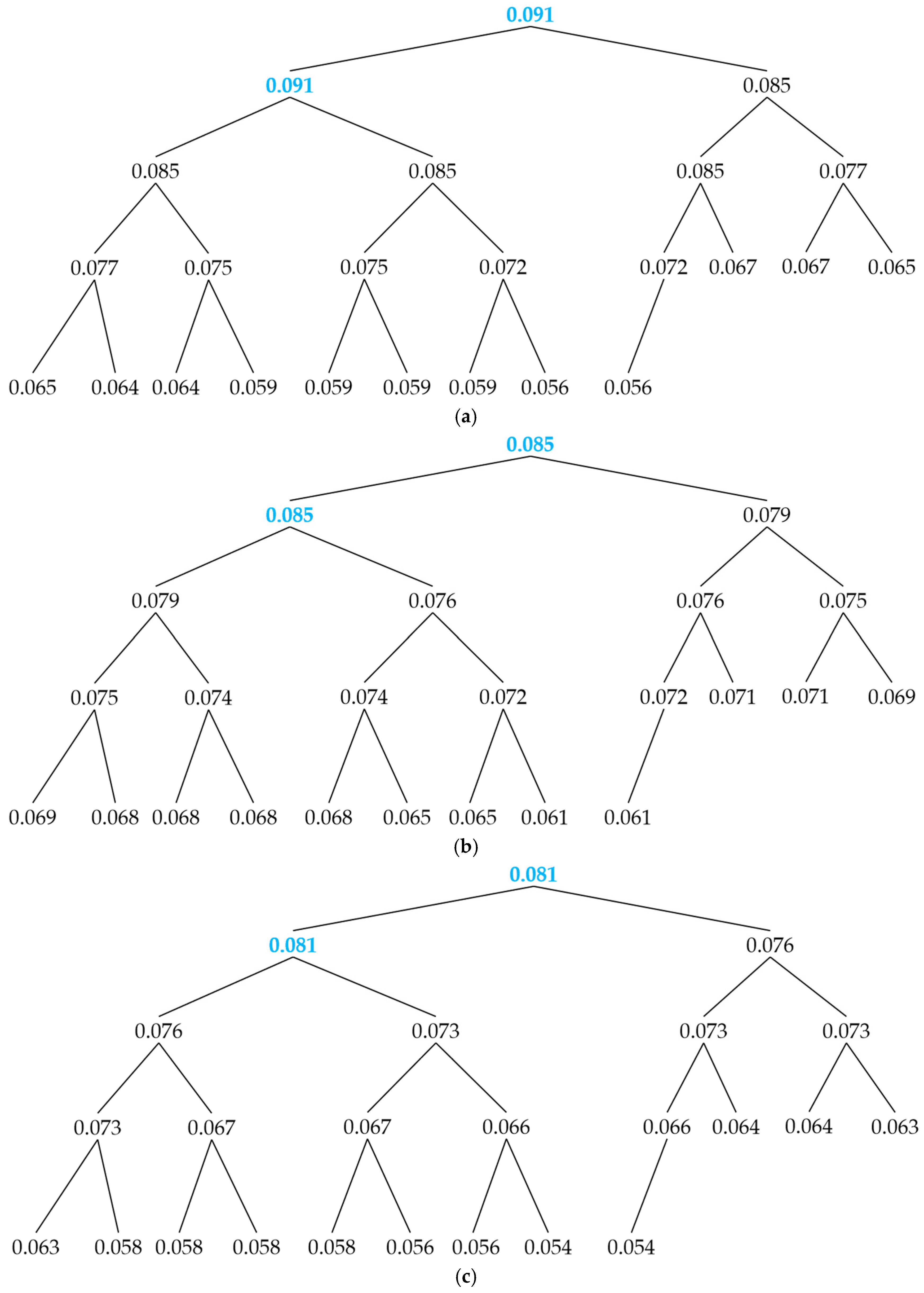
Analyze Table 8, Figure 11 and Table 9; it can be concluded that the experiment generates three tour route decision trees under the proposed experimental conditions, forming a tour route decision forest. Each decision tree corresponds to one sample hotel and contains 24 nodes, that is, 24 tour routes. In arbitrary decision tree, the traveling orders of the 24 tour routes are different, and the costs of sub-intervals are also different, resulting in the significant differences in the costs and cost indexes of tour routes, showing a fluctuating trend. Among them:

Figure 11a corresponds to the local optimal solutions of the first decision tree, which are routes $H_{(1)}$-$T_{(1)}$-$T_{(17)}$-$T_{(14)}$-$T_{(19)}$-$H_{(1)}$ and $H_{(1)}$-$T_{(19)}$-$T_{(14)}$-$T_{(17)}$-$T_{(1)}$-$H_{(1)}$, with the local optimal route cost of 11.000 km and the cost index of 0.091.

Figure 11b corresponds to the local optimal solutions of the second decision tree, which are routes $H_{(2)}$-$T_{(14)}$-$T_{(19)}$-$T_{(1)}$-$T_{(17)}$-$H_{(2)}$ and $H_{(2)}$-$T_{(17)}$-$T_{(1)}$-$T_{(19)}$-$T_{(14)}$-$H_{(2)}$, with the local optimal route cost of 11.700 km and the cost index of 0.085.

Figure 11c corresponds to the local optimal solutions of the third decision tree, which are routes $H_{(3)}$-$T_{(14)}$-$T_{(17)}$-$T_{(1)}$-$T_{(19)}$-$H_{(3)}$ and $H_{(3)}$-$T_{(19)}$-$T_{(1)}$-$T_{(17)}$-$T_{(14)}$-$H_{(3)}$, with the local optimal route cost of 12.400 km and the cost index of 0.081.

From the results, it can be concluded that among the three decision trees, the local optimal solution of the first decision tree is the global optimal solution in the decision forest, and its optimal tour route has the lowest cost. The tourist’s traveling along this route will generate the lowest transportation cost. Therefore, the most geographically optimal hotel recommended for the tourist is $H_{(1)}$: Hilton Garden Inn (South Third Section of the First Ring Road), and the optimal routes are $H_{(1)}$-$T_{(1)}$-$T_{(17)}$-$T_{(14)}$-$T_{(19)}$-$H_{(1)}$ and $H_{(1)}$-$T_{(19)}$-$T_{(14)}$-$T_{(17)}$-$T_{(1)}$-$H_{(1)}$, which proves the rationality of the constructed hotel recommendation algorithm and its ability to output the global optimal solution.

(4)

Through the experiment, we analyze the generalization and convergence performance of the decision forest algorithm, as well as the aggregation mechanism of route costs in the decision forest. Firstly, the constructed decision forest algorithm can adapt to any tourist interest conditions to output scenic spots, with good generalization performance. One tree in the decision forest represents one hotel within a tourism sub-region. When any tourist provides interests, the constructed matching algorithm can recommend precise scenic spots, and the IDFST algorithm can output the optimal routes within sub-intervals. Through linear iteration of sub-intervals and linear aggregation of route costs, the overall costs of different tour routes corresponding to the hotel are finally output, and then a decision tree corresponding to the hotel is generated. The nodes on the decision tree store the cost indexes of different tour routes. Thus, when there are changes in the city condition or tourists’ interests, the different decision forests within tourism sub-regions can all be output, and the optimal decision tree and hotel recommendation can be selected from the decision forest. Secondly, based on the constructed decision forest algorithm, the iteration of sub-intervals within each decision tree is linear, and the iteration of route costs is also linear. Therefore, when hotels and scenic spots are determined, they must be able to output the overall cost and cost index of each tour route, and then output the optimal solution of the decision tree through the decision tree sorting algorithm. Then, the optimal solution of the decision forest will be obtained when the optimal solutions of decision trees are obtained. The analysis of the decision forest algorithm logic shows that the algorithm ensures convergence to the global optimal solution, and the convergence rate is linear.

4.6. Results and Analysis of the Comparative Experiment

4.6.1. Experimental Conditions

The constructed hotel recommendation algorithm is based on the scenic spot recommendation and the optimal route planning, and it recommends the lowest transportation cost route and corresponding hotel to tourists. To verify the advantages of the constructed algorithm, we design comparative experiments to compare the hotel recommendation algorithm (PRA, Proposed Algorithm) with the conventional classical algorithms. Two sets of comparative experiments are designed, with the following experimental conditions:

(1)

To compare the results of the experimental group and the control group, we introduce the optimization rate model, as shown in Formula (10), in which $C_{\exp .}$ is the cost generated by the experimental group and $C_{con.}$ is the cost generated by the control group. The model represents the optimization degree of the experimental group compared to the control group. When ${\mu }_{(\exp .,con.)}>0$, it indicates that the experimental group is superior to the control group; when ${\mu }_{(\exp .,con.)}=0$, it indicates that the experimental group is equivalent to the control group; when ${\mu }_{(\exp .,con.)}<0$, it indicates that the control group is superior to the experimental group.

$${\mu }_{(\exp .,con.)}={\displaystyle \frac{C_{con.}-C_{\exp .}}{C_{con.}}}\times 100\%$$

(10)

(2)

The design of the first comparative experiment: The experimental group is set as the PRA. The centroid of the points distributed in space should be referenced to the coordinates of the most gathered points, or given higher weights. For points that are too discrete, their influencing weights should be reduced, or they should be directly removed as the noise data. The distribution of the scenic spots in the urban space is not linear or uniform, so the relatively gathered scenic spots should be the main factors in calculating the centroid, while the deviated scenic spots should be considered as the secondary factors. The control group uses the weighted centroid positioning algorithm (WCPA) to calculate the centroid of scenic spots, and then calculates the spatial closeness with the coordinates of each hotel to obtain the optimal hotel recommendation. We use the scenic spots and their coordinates as the initial data for calculating the optimal hotel location, and use WCPA to calculate the weighted centroid of the scenic spots. Then, by constructing the spatial closeness model between hotel and the centroid of scenic spots, the optimal hotel can be calculated. Formula (11) is the constructed weighted centroid positioning model, in which $L_c$ is the longitude of the weighted centroid of scenic spots, $B_c$ is the latitude of the weighted centroid of scenic spots, $l_{T(i)}$ is the longitude of the recommended scenic spot, $b_{T(i)}$ is the latitude of the recommended scenic spot, and ${\epsilon }_{T(i)}$ is the gathering weight of scenic spots. In this experiment, we set the weights ${\epsilon }_{T(i)}$ based on the degree of gathering of the recommended scenic spots, satisfying Formula (12), and set that the more gathered the scenic spots are, the higher the weights will be, and the more deviated the scenic spots are, the lower the weights will be. Formula (13) is the constructed spatial closeness model $f(H_{(i)},C_{T(i)})$ between the hotel and the weighted centroid of scenic spots, in which $L_{H(i)}$ and $B_{H(i)}$ are the latitude and longitude of the hotel, $L_{C_{T(i)}}$ and $B_{C_{T(i)}}$ are the latitude and longitude of the weighted centroid of scenic spots, and $\delta$ is the normalized parameter.

$$L_c={\displaystyle \sum _{i=1}^{\max i}{\epsilon }_{T(i)}\times l_{T(i)}}, B_c={\displaystyle \sum _{i=1}^{\max i}{\epsilon }_{T(i)}\times b_{T(i)}}$$

(11)

$${\displaystyle \sum _{i=1}^{\max i}{\epsilon }_{T(i)}}=1$$

(12)

$$f(H_{(i)},C_{T(i)})=\delta \times {\displaystyle \frac{1}{\sqrt{{\left(L_{H_{(i)}}-L_{C_{T(i)}}\right)}^2+{\left(B_{H_{(i)}}-B_{C_{T(i)}}\right)}^2}}}$$

(13)

(3)

The second comparative experiment: When recommending hotels, we use routes and route costs generated by hotels and scenic spots as the standard, and the core algorithm for constructing tour routes is the IDFST algorithm. Among the conventional algorithms for route planning, the greedy algorithm is a classic method that generates a path connecting the starting and ending points by local greedy search. The shortest path generated by the greedy algorithm may be a global optimal solution or a local optimal solution. In the comparative experiment, we use the tour route algorithm in constructing the hotel recommendation model as the experimental group (PRA, Proposed Algorithm), and the greedy mountain climbing algorithm (GMCA) and greedy breadth first search algorithm (GBFSA) as the control group. The constructed sub-intervals with the same hotel and scenic spots are used as the data conditions to calculate sub-interval route cost $C_{Rou(i)}$ and cost index ${\delta }_{Rou(i)}$ under each algorithm condition. The optimal tour route is used as the standard to calculate the tour route cost $C_{T\cdot Rou(i)}$ and cost index ${\delta }_{T\cdot Rou(i)}$ of each algorithm.

4.6.2. Results and Analysis of the First Comparative Experiment

According to Figure 7, among the four recommended scenic spots, $T_{(1)}$: People’s Park, $T_{(14)}$: Qingyang Palace, and $T_{(17)}$: Kuanzhai Alley have a high degree of gathering, while $T_{(19)}$: Roman Holiday Plaza is relatively scattered and far away. According to the agreement on the gathering weight ${\epsilon }_{T(i)}$ of scenic spots, we set the weight of each scenic spot as ${\epsilon }_{T(1)}={\epsilon }_{T(14)}={\epsilon }_{T(17)}=0.3$, ${\epsilon }_{T(19)}=0.1$. We output the weighted centroid $C_{T(i)}$ of scenic spots with latitude and longitude by the weighted centroid positioning algorithm, and then calculate the closeness between hotel $H_{(i)}$ and the weighted centroid. The candidate hotels are $H_{(i)}$: {$H_{(1)}$: Hilton Garden Inn (South Third Section of the First Ring Road); $H_{(2)}$: Ji Hotel (Chengdu Kuanzhai Alley West Branch); $H_{(3)}$: Tianyou International Hotel (Chengdu Jinli Branch).

Table 10. The latitude and longitude of the weighted centroid of scenic spots output by the algorithm, as well as the closeness between the hotels and the weighted centroid of scenic spots.

	Candidate Hotel			Recommended Scenic Spot				Weighted Centroid	Hotel Closeness Degree f (H(i),CT(i))
	H(1)	H(2)	H(3)	T(1)	T(14)	T(17)	T(19)	CT(i)
$L$	104.054	104.030	104.022	104.057	104.042	104.053	104.042	104.050	H(1)	H(2)	H(3)
$B$	30.633	30.669	30.646	30.657	30.660	30.663	30.637	30.658	0.399	0.439	0.332

shows the latitude and longitude of the weighted centroid of scenic spots output by the algorithm, as well as the closeness between the hotels and the weighted centroid of scenic spots. According to the results in Table 10, the hotel with the highest degree of closeness with the weighted centroid is the $H_{(2)}$: Ji Hotel (Chengdu Kuanzhai Alley West Branch).

We set the optimal hotels output by the experimental group and the control group as the starting point and the ending point, respectively, and use the four recommended scenic spots as route nodes. The experiment outputs the optimal tour routes, respectively. It is stipulated that all feasible route costs $C_{Rou(i)}$ and feasible route cost indexes ${\delta }_{Rou(i)}$ within the tourism sub-regions of the experimental group and the control group are identical.

Table 11. The comparison of the sub-interval optimal route costs and the optimal tour route costs between the experimental group and the control group.

	Optimal Tour Route	Sub-Interval Optimal Tour Route Cost ${\mathit{C}}_{\mathit{R}\mathit{o}\mathit{u}(\mathit{i})}^{\mathit{o}\mathit{p}\mathit{t}}$ (km)					Optimal Tour Route Cost ${\mathit{C}}_{\mathit{T}\cdot \mathit{R}\mathit{o}\mathit{u}(\mathit{i})}^{\mathit{o}\mathit{p}\mathit{t}}$ (km)	Optimization Rate
		${\mathit{S}}_{\mathit{I}(1)}$	${\mathit{S}}_{\mathit{I}(2)}$	${\mathit{S}}_{\mathit{I}(3)}$	${\mathit{S}}_{\mathit{I}(4)}$	${\mathit{S}}_{\mathit{I}(5)}$	${\mathit{T}}_{\mathit{R}\mathit{o}\mathit{u}(\mathit{i})}$	${\mathit{\mu }}_{(\mathbf{PRA},\mathbf{WCPA})}$
PRA	h1-1,17,14,19-h1	3.4	1.1	2.2	2.9	1.4	11.0	5.98%
	h1-19,14,17,1-h1	1.4	2.9	2.2	1.1	3.4	11.0
WCPA	h2-14,19,1,17-h2	1.8	2.9	3.3	1.1	2.6	11.7
	h2-17,1,19,14-h2	2.6	1.1	3.3	2.9	1.8	11.7

shows the comparison of sub-interval optimal route costs and the optimal tour route costs between the experimental group and the control group.

Table 12. The comparison of sub-interval optimal route cost indexes between the experimental group and the control group, as well as the comparison of cost indexes for the optimal tour routes.

	Optimal Tour Route	Sub-Interval Optimal Tour Route Cost Index ${\mathit{\delta }}_{\mathit{R}\mathit{o}\mathit{u}(\mathit{i})}^{\mathit{o}\mathit{p}\mathit{t}}$					Optimal Tour Route Cost Index ${\mathit{\delta }}_{\mathit{T}\cdot \mathit{R}\mathit{o}\mathit{u}(\mathit{i})}^{\mathit{o}\mathit{p}\mathit{t}}$
		${\mathit{S}}_{\mathit{I}(1)}$	${\mathit{S}}_{\mathit{I}(2)}$	${\mathit{S}}_{\mathit{I}(3)}$	${\mathit{S}}_{\mathit{I}(4)}$	${\mathit{S}}_{\mathit{I}(5)}$	${\mathit{T}}_{\mathit{R}\mathit{o}\mathit{u}(\mathit{i})}$
PRA	h1-1,17,14,19-h1	0.294	0.909	0.455	0.345	0.714	0.091
	h1-19,14,17,1-h1	0.714	0.345	0.455	0.909	0.294	0.091
WCPA	h2-14,19,1,17-h2	0.556	0.345	0.303	0.909	0.385	0.085
	h2-17,1,19,14-h2	0.385	0.909	0.303	0.345	0.556	0.085

shows the comparison of the sub-interval optimal route cost indexes between the experimental group and the control group, as well as the comparison of cost indexes for the optimal tour routes.

Figure 12 shows the cost trend and cost index trend of the optimal tour routes for the experimental group and the control group. Figure 12a–d show the trend comparison of the route costs between the experimental group and the control group. Figure 12a,b, respectively, show the sub-interval optimal route costs (blue data bars) and the optimal tour route costs (green data bars) of the two optimal routes in the experimental group. Figure 12c,d, respectively, show the sub-interval optimal route costs (brown data bars) and the optimal tour route costs (green data bars) of the two optimal routes in the control group. Figure 12e–h show the trend comparison of the route cost indexes between the experimental group and the control group. Figure 12e,f, respectively, show the sub-interval optimal route cost indexes (blue data bar) and the optimal tour route cost indexes (green data bar) of the two optimal routes in the experimental group. Figure 12g,h, respectively, show the sub-interval optimal route cost indexes (brown data bar) and the optimal tour route cost indexes (green data bar) of the two optimal routes in the control group.

The following conclusions are drawn from the analysis of the first set of comparative experiments:

(1)

According to the analysis of Table 10, the optimal hotel recommended by WCPA for the control group is the $H_{(2)}$: Ji Hotel (Chengdu Kuanzhai Alley West Branch). Its basic logic is reasonable and feasible, which measures the aggregation and deviation degree of scenic spots to be visited, and determines the weight of each scenic spot, then calculates the weighted centroid positioning point of the scenic spots. This method can bring the weighted centroid closer to the gathered scenic spots, taking into account the geographical advantages of most gathered scenic spots. On this basis, it calculates the closeness between hotels and the centroid. The higher the closeness degrees are, the higher the closeness between hotels and the gathered scenic spots will be. That is, the optimal hotel is located closer to most scenic spots, which is in line with the common habit of tourists when traveling. The tourists usually book a hotel that is closer to most scenic spots. However, this method has limitations as it determines the centroid and hotel closeness degree from the perspective of spatial average distance without considering the transportation distance between hotels and various scenic spots, as well as the route costs incurred by tourists when visiting scenic spots in certain sequence. When measured from the perspective of tour route costs, a hotel recommended by the centroid positioning method may not be the global optimal solution.

(2)

According to the analysis of the data in Table 11 and Table 12, the constructed algorithm measures the cost of tour routes between hotels and scenic spots, as well as the overall cost of tour routes, considering the order of tourists’ visits, with the goal of minimizing tourism transportation costs to the greatest extent possible. When analyzing the comparison of route costs, the overall costs of the two optimal tour routes in the experimental group are lower than those of the control group, and cost indexes are higher than those of the control group. Compared with the control group, the optimization rate of route costs in the experimental group reaches 5.98%. The optimal routes output by the experimental group are $H_{(1)}$-$T_{(1)}$-$T_{(17)}$-$T_{(14)}$-$T_{(19)}$-$H_{(1)}$ and $H_{(1)}$-$T_{(19)}$-$T_{(14)}$-$T_{(17)}$-$T_{(1)}$-$H_{(1)}$, with a route cost of 11.0 km and a cost index of 0.091. The optimal routes output by the control group are $H_{(2)}$-$T_{(14)}$-$T_{(19)}$-$T_{(1)}$-$T_{(17)}$-$H_{(2)}$ and $H_{(2)}$-$T_{(17)}$-$T_{(1)}$-$T_{(19)}$-$T_{(14)}$-$H_{(2)}$, with a route cost of 11.7 km and a cost index of 0.085. The results indicate that the constructed algorithm can generate the lowest tourism transportation cost, which is better than the control group algorithm.

(3)

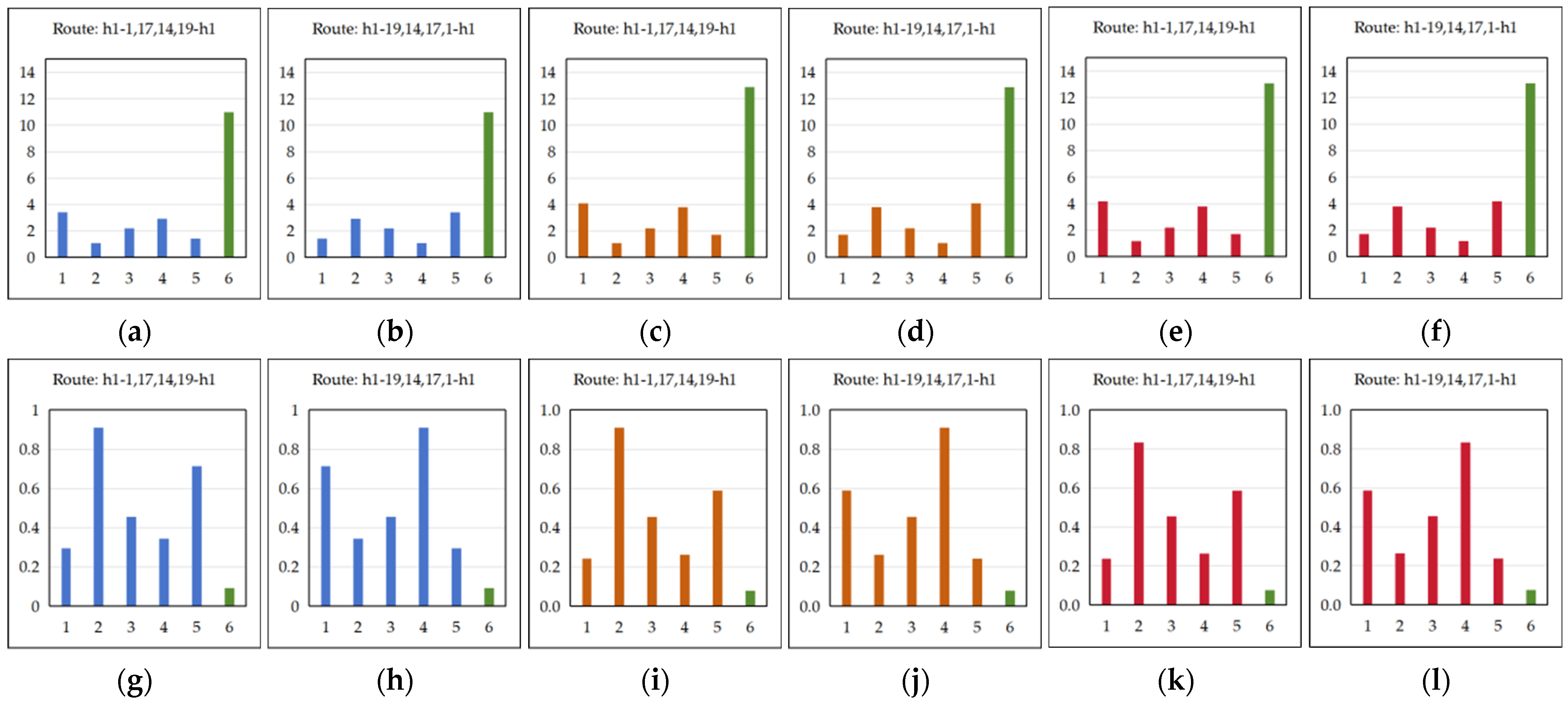
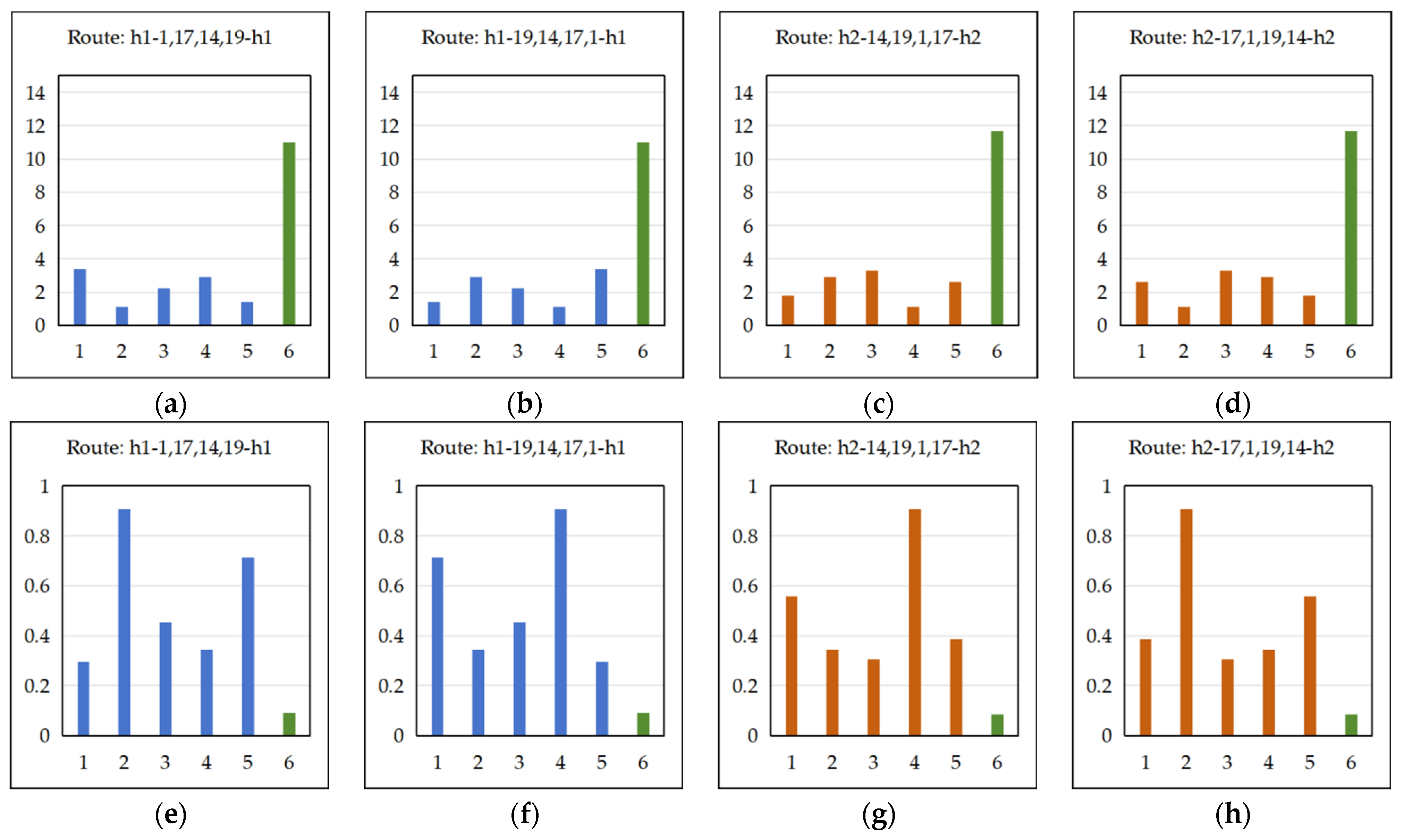
From the results in Figure 12, it can be concluded that the experimental group and the control group generate different optimal tour routes, and the optimal costs and cost indexes generated by each route within sub-intervals show a fluctuating trend. This indicates that the constructed algorithm is based on the different sub-interval orders and combinations when generating tour routes, which conforms to the habit of tourist visiting scenic spots in a certain order. By comparison, it can be concluded that the green data bars in Figure 12a,b are lower than those in Figure 12c,d, indicating that the costs of tour routes in the experimental group are lower than those in the control group. Compared to Figure 12g,h, Figure 12e,f show higher green data columns, indicating that the cost indexes of tour routes in the experimental group are higher than those in the control group. From the analysis and comparison chart, it can be concluded that the constructed algorithm is superior to the control group algorithm.

4.6.3. Results and Analysis of the Second Comparative Experiment

We use the hotel recommendation algorithm based on IDFST as the experimental group (PRA), and the commonly used greedy mountain climbing algorithm (GMCA) and greedy BFS algorithm (GBFSA, Greedy Breadth First Search Algorithm) for route planning as the control group. To ensure fairness of the experiment, the optimal hotel, $H_{(1)}$: Hilton Garden Inn (South Third Section of the First Ring Road), is selected as the starting and the ending points of the tour route, while the recommended scenic spots remain unchanged. The experimental setup is as follows: the experimental group and the control group search for the cost and cost index of each sub-interval, and then search for the cost and cost index of the optimal tour route. The cost and cost index of each sub-interval are compared to obtain the optimization rate. Then, the cost and cost index of the optimal tour route are compared to obtain the optimization rate.

Table 13. The sub-interval route costs, sub-interval route cost indexes, and optimization rates output by the experimental group and the control group.

	Sub-Interval Route Cost ${\mathit{C}}_{\mathit{R}\mathit{o}\mathit{u}(\mathit{i})}$			Sub-Interval Route Cost Index ${\mathit{\delta }}_{\mathit{R}\mathit{o}\mathit{u}(\mathit{i})}$			μ(PRA,GMCA)	μ(PRA,GBFSA)
	PRA	GMCA	GBFSA	PRA	GMCA	GBFSA
H(1)T(1)	3.4	4.1	4.2	0.294	0.244	0.238	17.07%	19.05%
H(1)T(14)	3.7	4.7	4.6	0.270	0.213	0.217	21.28%	19.57%
H(1)T(17)	3.9	4.4	4.8	0.256	0.227	0.208	11.36%	18.75%
H(1)T(19)	1.4	1.7	1.7	0.714	0.588	0.588	17.65%	17.65%
T(1)T(14)	2.5	2.6	2.7	0.400	0.385	0.370	3.85%	7.41%
T(1)T(17)	1.1	1.1	1.2	0.909	0.909	0.833	0.00%	8.33%
T(1)T(19)	3.3	4	3.7	0.303	0.250	0.270	17.50%	10.81%
T(14)T(17)	2.2	2.2	2.2	0.455	0.455	0.455	0.00%	0.00%
T(14)T(19)	2.9	3.8	3.8	0.345	0.263	0.263	23.68%	23.68%
T(17)T(19)	4.3	4.7	4.3	0.233	0.213	0.233	8.51%	0.00%

shows the sub-interval route costs, sub-interval route cost indexes, and the optimization rates output by the experimental group and the control group.

Figure 13 shows the fluctuation trend of the costs, cost indexes, and the optimization rates in each sub-interval of the experimental group and the control group. Figure 13a shows the trend and comparison of the route costs between the experimental group and the control group in each sub-interval, while Figure 13b shows the trend and comparison of the route cost indexes between the experimental group and the control group in each sub-interval. The blue data column represents PRA, the orange data column represents GMCA, and the green data column represents GBFSA. Figure 13c shows the cost optimization rates of the experimental group PRA compared to the control group GMCA in each sub-interval, and Figure 13d shows the cost optimization rates of the experimental group PRA compared to the control group GBFSA in each sub-interval.

Starting from $H_{(1)}$: Hilton Garden Inn (South Third Section of the First Ring Road), the four recommended scenic spots are used as route nodes. The experimental group algorithm and the control group algorithm are used to output the global optimal tour routes, respectively. The sub-interval route costs, sub-interval route cost indexes, tour route costs, and tour route cost indexes of the optimal tour routes are compared, and the route cost optimization rates are obtained.

Table 14. The sub-interval route costs, optimal tour route costs, and route cost optimization rates of the optimal tour routes output by the experimental group and the control group.

	Optimal Tour Route	Sub-Interval Route Cost ${\mathit{C}}_{\mathit{R}\mathit{o}\mathit{u}(\mathit{i})}^{\mathit{o}\mathit{p}\mathit{t}}$					Optimal Tour Route Cost ${\mathit{C}}_{\mathit{T}\cdot \mathit{R}\mathit{o}\mathit{u}(\mathit{i})}^{\mathit{o}\mathit{p}\mathit{t}}$	Route Cost Optimization Rate
		${\mathit{S}}_{\mathit{I}(1)}$	${\mathit{S}}_{\mathit{I}(2)}$	${\mathit{S}}_{\mathit{I}(3)}$	${\mathit{S}}_{\mathit{I}(4)}$	${\mathit{S}}_{\mathit{I}(5)}$	${\mathit{T}}_{\mathit{R}\mathit{o}\mathit{u}(\mathit{i})}$	μ(PRA,GMCA)	μ(PRA,GBFSA)
PRA	h1-1,17,14,19-h1	3.4	1.1	2.2	2.9	1.4	11.0	14.73%	16.03%
	h1-19,14,17,1-h1	1.4	2.9	2.2	1.1	3.4	11.0
GMCA	h1-1,17,14,19-h1	4.1	1.1	2.2	3.8	1.7	12.9
	h1-19,14,17,1-h1	1.7	3.8	2.2	1.1	4.1	12.9
GBFSA	h1-1,17,14,19-h1	4.2	1.2	2.2	3.8	1.7	13.1
	h1-19,14,17,1-h1	1.7	3.8	2.2	1.2	4.2	13.1

shows the sub-interval route costs, the optimal tour route costs, and route cost optimization rates of the optimal tour routes output by the experimental group and the control group.

Table 15. The sub-interval cost indexes and optimal tour route cost indexes of the optimal tour routes output by the experimental group and the control group.

	Optimal Tour Route	Sub-Interval Route Cost Index ${\mathit{\delta }}_{\mathit{R}\mathit{o}\mathit{u}(\mathit{i})}^{\mathit{o}\mathit{p}\mathit{t}}$					Optimal Tour Route Cost Index ${\mathit{\delta }}_{\mathit{T}\cdot \mathit{R}\mathit{o}\mathit{u}(\mathit{i})}^{\mathit{o}\mathit{p}\mathit{t}}$
		${\mathit{S}}_{\mathit{I}(1)}$	${\mathit{S}}_{\mathit{I}(2)}$	${\mathit{S}}_{\mathit{I}(3)}$	${\mathit{S}}_{\mathit{I}(4)}$	${\mathit{S}}_{\mathit{I}(5)}$	${\mathit{T}}_{\mathit{R}\mathit{o}\mathit{u}(\mathit{i})}$
PRA	h1-1,17,14,19-h1	0.294	0.909	0.455	0.345	0.714	0.091
	h1-19,14,17,1-h1	0.714	0.345	0.455	0.909	0.294	0.091
GMCA	h1-1,17,14,19-h1	0.244	0.909	0.455	0.263	0.588	0.078
	h1-19,14,17,1-h1	0.588	0.263	0.455	0.909	0.244	0.078
GBFSA	h1-1,17,14,19-h1	0.238	0.833	0.455	0.263	0.588	0.076
	h1-19,14,17,1-h1	0.588	0.263	0.455	0.833	0.238	0.076

shows the sub-interval cost indexes and the optimal tour route cost indexes of the optimal tour routes output by the experimental group and the control group. Figure 14 shows the cost trend and cost index trend of the optimal tour routes for the experimental group and the control group. Figure 14a–f show the sub-interval route costs and tour route costs of the optimal tour routes output by the experimental group and the control group. Among them, Figure 14a,b correspond to the experimental group PRA, in which the blue data columns represent sub-interval costs and the green data columns represent tour route costs; Figure 14c,d correspond to GMCA of the control group, in which the orange data columns represent sub-interval costs and the green data columns represent tour route costs; Figure 14e,f correspond to the control group GBFSA, in which the red data columns represent sub-interval costs and the green data columns represent tour route costs. Figure 14g–l show sub-interval cost indexes and tour route cost indexes of the optimal tour routes output by the experimental group and the control group. Among them, Figure 14g,h correspond to the experimental group PRA, with the blue data columns representing sub-interval cost indexes and green data columns representing tour route cost indexes; Figure 14i,j correspond to the GMCA of the control group, in which the orange data columns represent sub-interval cost indexes and the green data columns represent tour route cost indexes; Figure 14k,l correspond to the control group GBFSA, with the red data columns representing sub-interval cost indexes and the green data columns representing tour route cost indexes.

The following conclusions are drawn from the analysis of the second set of comparative experiments:

(1)

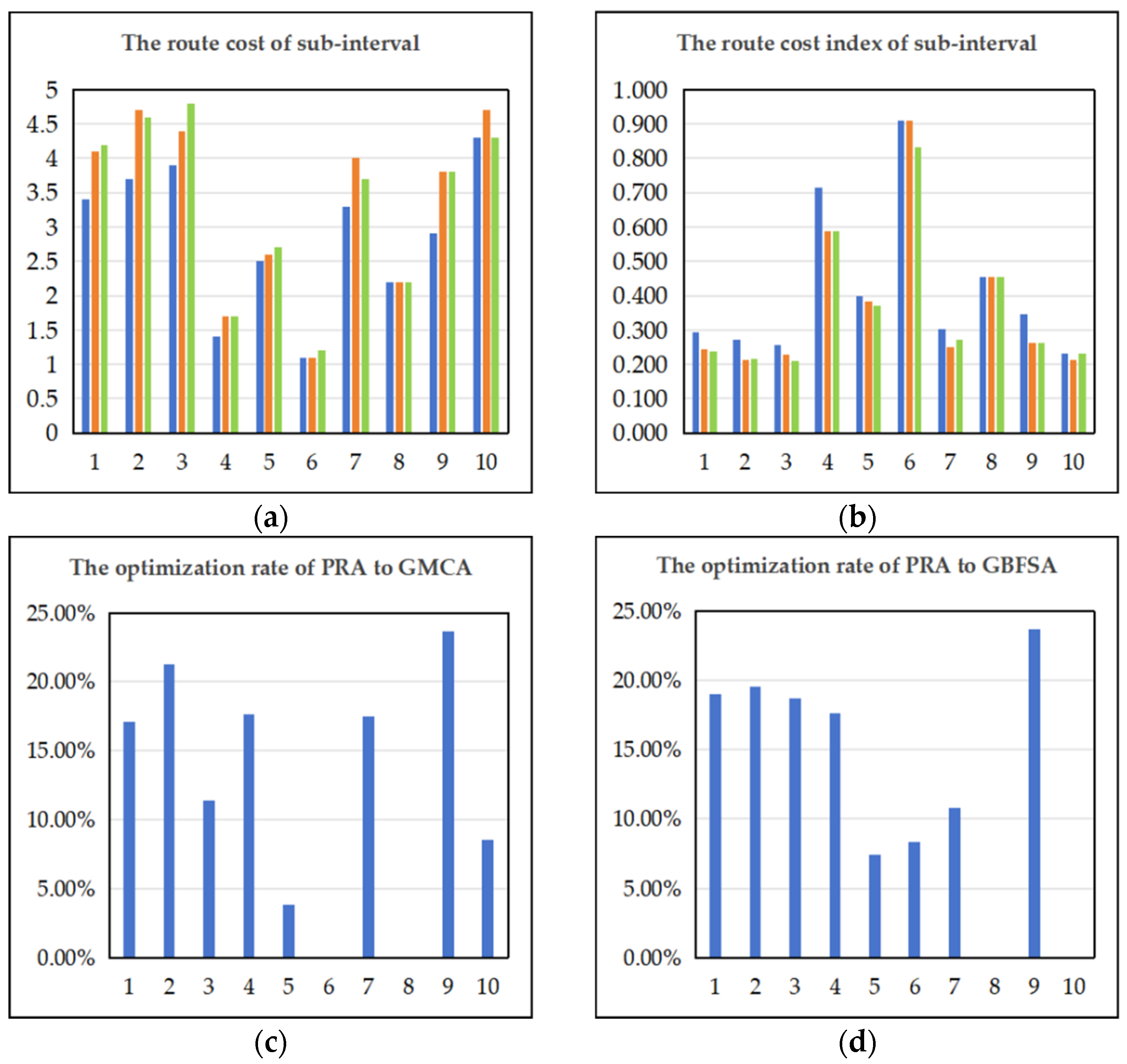
According to the analysis of Table 13 and Figure 13, it can be concluded that the experimental group and the control group generate different route costs in each sub-interval, and the bar charts all show the fluctuating trend. After comparison, it can be concluded that the experimental group algorithm generates lower route costs and higher route cost indexes in each sub-interval compared to the control group algorithms, indicating that the constructed algorithm is superior in searching for the lowest cost route compared to the traditional algorithms. From the perspective of optimization rate, PRA has the highest optimization rate of 23.68% in sub-interval $T_{(14)}{T}_{(19)}$ compared to GMCA, and the lowest optimization rate of 0% in sub-intervals $T_{(1)}{T}_{(17)}$ and $T_{(14)}{T}_{(17)}$. However, overall, the optimization rates are greater than 0. Compared to GBFSA, PRA has the highest optimization rate on sub-interval $T_{(14)}{T}_{(19)}$, at 23.68%, and the lowest optimization rate on sub-intervals $T_{(14)}{T}_{(17)}$ and $T_{(17)}{T}_{(19)}$, at 0%. However, overall, the optimization rates are greater than 0. PRA costs, represented by the blue data columns in Figure 13a, are lower than or equal to GMCA (orange) and GBFSA (green), while PRA cost indexes, represented by the blue data columns in Figure 13b, are higher than or equal to GMCA (orange) and GBFSA (green). The optimization rates of Figure 13c,d are all values greater than or equal to 0, and there are no negative values. Therefore, in terms of cost and optimization rate, the constructed algorithm is superior to the control group.

(2)

According to the analysis of Table 14 and Table 15, and Figure 14, it can be concluded that when the starting point, ending point, and nodes of tour route are determined, the optimal routes output by the experimental group and the control group are all $H_{(1)}$-$T_{(1)}$-$T_{(17)}$-$T_{(14)}$-$T_{(19)}$-$H_{(1)}$ and $H_{(1)}$-$T_{(19)}$-$T_{(14)}$-$T_{(17)}$-$T_{(1)}$-$H_{(1)}$, but, due to the different algorithm principles and search methods, tour route costs and cost indexes output by the experimental group and the control group are different. Among them, PRA outputs the route cost of 11.0 km and cost index of 0.091 in the experimental group, GMCA outputs route cost of 12.9 km and cost index of 0.078 in the control group, and GBFSA outputs route cost of 13.1 km and cost index of 0.076 in the control group. From the perspective of tour route cost optimization rate, the optimization rate of PRA compared to GMCA is 14.73%, and the optimization rate of PRA compared to GBFSA is 16.03%. In Figure 14, costs and cost indexes of sub-intervals as well as tour routes output by the experimental group and the control group are different. The green data columns in Figure 14a,b represent lower route costs than those in Figure 14c–f, and the green data columns in Figure 14g,h represent higher route cost indexes than those in Figure 14i–l. This indicates that the constructed algorithm generates lower costs and higher cost indexes for tour routes compared to the control group algorithms, and is superior to the control group algorithms.

(3)

We analyzed the reasons for the differences between the experimental group and the control group. As the constructed algorithm optimizes the DFS algorithm, removes backtracking edges (negative edges), and traverses all feasible routes to ultimately output sub-interval optimal solution, the resulting route is the global optimal solution. The control group algorithms are the commonly used methods for route search, based on the greedy idea of finding the edge with the lowest cost or the point closest to the endpoint every time when the next node is searched. This method cannot guarantee that the searched route will always be the global optimal solution; it may be a local optimal solution. Based on the above analysis, the constructed algorithm can find the global optimal solution, ensure the optimal hotel recommendation result, minimize the route cost, effectively reduce tourists’ traveling costs, and improve tourists’ satisfaction.

4.6.4. Analysis of Algorithm Scalability and Structural Performance

In this experiment, we chose specific experimental conditions (e.g., one sample city and one tourist providing interest data) to demonstrate the rationality and advantages of the algorithm. The main reasons are as follows:

(1)

Analysis from the perspective of algorithmic logic. The goal of both the experimental group and the control group is to recommend hotels, but the algorithm logics are fundamentally different. Firstly, the weighted centroid positioning algorithm (WCPA) sets weights based on the degree of scenic spot gathering, and outputs hotel location near the gathering of scenic spots with higher weights. It considers the distance between tourists and important scenic spots and ignores the overall route cost generated during the tour process. Essentially, it does not model the transportation cost of tourists’ traveling, and the recommended hotel is not the optimal solution. Secondly, compared to the Greedy Mountain Climbing Algorithm (GMCA) and the Greedy Breadth First Search Algorithm (GBFSA), the constructed IDFST algorithm is more logically superior. The routes output in each sub-interval are better than the two algorithms, and the cost of the entire tour route is also the lowest, corresponding to the optimal solution. When the city conditions change, only external conditions such as roads, road nodes, and distances between nodes in the city change, while the algorithm logics of the experimental and control groups do not change. The experimental group still has the characteristics and ability to output the optimal solution, and is superior to the control group algorithms. Therefore, implementing the constructed algorithm in any city can output the lowest cost tour routes and the optimal hotel recommendation results, unaffected by the changes in the city’s geospatial environment.

(2)

Analysis from the perspective of tourists. In the constructed algorithm, the influence of tourists on the algorithm is reflected in the fact that different tourists’ interests may output different scenic spots. However, from the perspective of the constructed hotel recommendation algorithm, the algorithm logic of the IDFST algorithm remains unchanged in outputting the optimal route and recommending the optimal hotel. In the same urban geographic environment, external conditions such as urban roads, road nodes, and distances between nodes remain unchanged. When recommending different scenic spots to different tourists within the same tourism sub-region, it is certain to output the corresponding scenic spot recommendation results and the optimal hotel recommendation results under the tourists’ interest conditions, while ensuring the lowest cost of tour route. Under this condition, the algorithm logics of the experimental group and the control group remain unchanged, and hotel as well as tour routes output by the experimental group must also be the optimal, which is determined by the underlying logic of the algorithm and is not affected by changes in tourists. Based on the above analysis, the constructed algorithm also has advantages compared to the control group when there are changes in tourists.

(3)

The constructed hotel recommendation algorithm is fundamentally different from the traditional recommendation algorithms, as it achieves the optimal hotel recommendations by two modules: the spatial clustering to form tourism sub-regions and the optimal route costs within tourism sub-regions. Therefore, the goal of the constructed ISTING-AGNES clustering algorithm is to generate tourism sub-regions, rather than aiming to improve the performance of clustering algorithm itself. That is, as long as the reasonable tourism sub-regions required for generating the hotel recommendation models are generated, the ISTING-AGNES clustering algorithm is feasible without the need for benchmark testing, ablation experiments, etc., to verify the performance of the clustering algorithm.

(4)

Based on the above analysis, the constructed algorithm has high scalability. When there are changes in the city conditions or tourists, the algorithm is superior to the control group algorithms in terms of underlying logic design, and can still obtain better results than the control group when external conditions change. Therefore, the advantages of the constructed algorithm can be demonstrated merely through specific experimental conditions, without the need to change the experimental environment for repeated experiments. Also, the statistical significance analysis and the validation on multiple datasets are not needed.

(5)

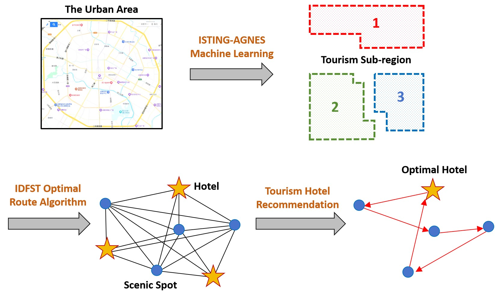
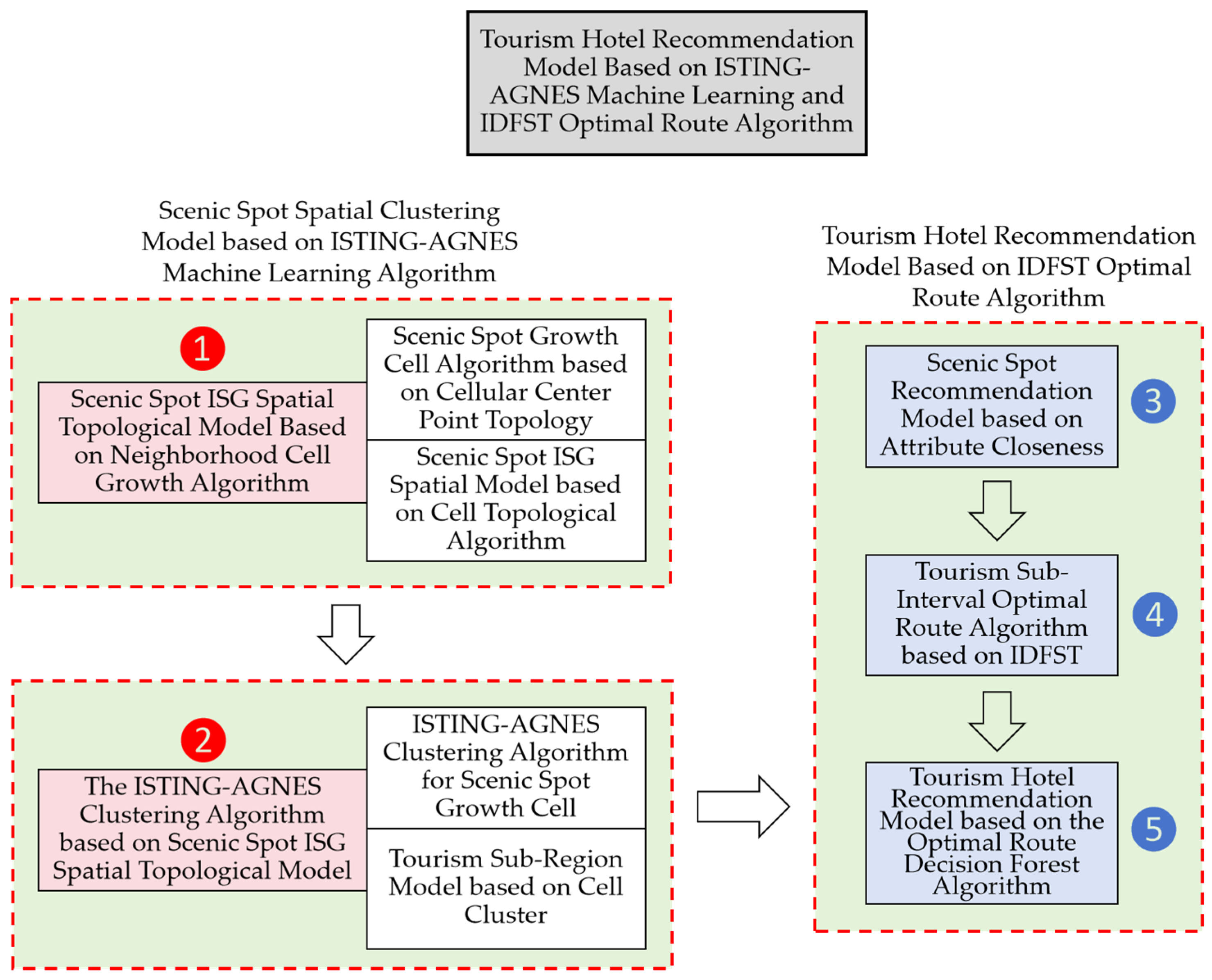
Analysis of the algorithm structural performance. The constructed algorithm model consists of the ISG spatial topological model, the ISTING-AGNES clustering algorithm, the scenic spot recommendation model based on attribute closeness, the IDFST route optimization algorithm, and the hotel recommendation model based on decision forest. Each module is the precondition for the next module, and the algorithm logic cannot be reversed or skipped. The process must be executed in the order shown in Figure 15, and each module has an irreplaceable role. Deleting any module or changing the algorithm process will affect the final hotel recommendation result, resulting in the output hotel not being the global optimal solution. Therefore, the constructed complete algorithm process is a pattern of “series connection” of the modules, as well as one-way flow of algorithms, and then outputting the final result, rather than the “parallel connection” of the modules and mutual interaction between modules to output the result. Each module is equally important and has the same contribution to the final result.

5. Conclusions

5.1. Summary of the Work

In response to the problem of hotel recommendation in tourism activities and research background, we construct a tourism hotel recommendation model based on ISTING-AGNES machine learning and the IDFST optimal route algorithm from a new research perspective. The recommendation model no longer uses traditional hotel attributes and service evaluation as the recommendation indicators, but, instead, takes the spatial cost generated between a hotel and scenic spots as the standard, establishing a hotel recommendation model with the optimal spatial location and the lowest travel route cost. We firstly construct a scenic spot spatial clustering model based on the ISTING-AGNES machine learning algorithm, which includes a scenic spot ISG spatial topological model based on the neighborhood cell growth algorithm and an ISTING-AGNES clustering algorithm based on scenic spot ISG spatial topological model. The city is divided into sub-regions to reduce computational and tourism cost dimensions. Then, within a tourism sub-region, we construct a tourism hotel recommendation model based on the IDFST optimal route algorithm, including a scenic spot recommendation model based on attribute closeness algorithm, a tourism sub-interval optimal route algorithm based on IDFST, and a tourism hotel recommendation model based on the optimal route decision forest algorithm, achieving the best geographical location and hotel recommendation with the lowest tour route cost. The experimental results show that the constructed algorithm can output hotel with the best geographical location and the lowest travel route cost. Under the set experimental conditions, compared with hotels recommended by the weight centroid positioning method, the cost optimization rate reaches 5.98%. Compared with greedy mountain climbing algorithm and greedy BFS algorithm, the cost optimization rates reach 14.73% and 16.03%, respectively. This proves that the constructed algorithm is feasible and advantageous.

5.2. Future Work

The constructed hotel recommendation algorithm is to perform dimensionality reduction on urban space, divide it into tourism sub-regions, and recommend hotels within sub-regions. In the next step of research, we will carry out the following tasks. Firstly, as candidate hotels and scenic spots are provided when constructing the hotel recommendation algorithm, the selection of hotels and scenic spots is not studied. We will further conduct research studies on the selection of candidate hotels and scenic spots in the modeling conditions, to determine hotels and scenic spots that better meet the needs and interests of tourists, and to improve adaptability of the algorithm. Secondly, in order to improve computational efficiency and reduce travel costs for tourists, we perform dimensionality reduction on the urban space during modeling, dividing it into multiple tourism sub-regions. When certain tourists might be interested in scenic spots outside a certain sub-region and the interested scenic spots are included in the list of scenic spots to be visited, it is necessary to include them in the modeling scope of the hotel recommendation algorithm. The modeling conditions, spatial range, sub-interval span, route span, etc., will all change. Therefore, further optimization of the model is needed to meet the new needs of potential tourists. Thirdly, when constructing the hotel recommendation algorithm, we use the universal cost of tour routes as the standard. Under the actual tourism conditions, tourists could have diverse forms of transportation choices. In the next step of research, different transportation modes could be used as modeling conditions to provide more suitable data conditions for hotel recommendations in the tourism scenario. Fourthly, the constructed scenic spot recommendation algorithm is based on the current interests and needs of tourists, while the route algorithms and hotel recommendation algorithms are constructed based on the static road traffic data as conditions, which can help tourists get recommendations on the best scenic spots and hotels to a certain extent. The algorithm does not take into account the possible changes in traffic conditions and the changing interests of tourists. When there are changes in transportation, congestion, etc., tourists may change their travel routes in real time. When tourists’ interests change, the recommended scenic spots and hotels may also change. Therefore, in the next step of the application research and system development of the algorithm, we will use the possible changes in traffic conditions and the real-time interests of tourists as the modeling conditions to design a real-time recommendation model and provide better services for tourists.

References

- Lv, L.; Zhang, Y.; Liao, J.; Chen, J.; Dai, G. How personalized recommendations influence customers’ sustainable hotels booking: The role of environmental identity label perception. Int. J. Hosp. Manag. 2026, 137, 104701. [Google Scholar] [CrossRef] [Scilit]
- Saeed, A.S.; Alamgir, Z. FCASR: A feature and content-aware service recommender for personalized hotel recommendations using big data. J. Big Data 2025, 12, 259. [Google Scholar] [CrossRef] [Scilit]
- Prakash, A.; Shukla, R. Enhancing hotel consumer recommendation decisions: A rough set approach for predictive analysis of online reviews. Inf. Sci. 2025, 719, 122456. [Google Scholar] [CrossRef] [Scilit]
- Remountakis, M.; Kotis, K.; Kourtzis, B.; Tsekouras, G.E. Using ChatGPT and Persuasive Technology for Personalized Recommendation Messages in Hotel Upselling. Information 2023, 14, 504. [Google Scholar] [CrossRef] [Scilit]
- Puttinaovarat, S.; Arayalert, C.S.; Saetang, W. GIS-Based Personalized Tourism Recommendation Using Association Rule Mining to Support Sustainable Tourism. Sustainability 2026, 18, 3145. [Google Scholar] [CrossRef] [Scilit]
- Hsieh, Y.C.; Lu, L.C.; Ku, Y.F. Review Evaluation for Hotel Recommendation. Electronics 2023, 12, 4673. [Google Scholar] [CrossRef] [Scilit]
- Wang, X.; Wang, S.; Zhang, H.; Wang, J.Q.; Li, L. The Recommendation Method for Hotel Selection Under Traveller Preference Characteristics: A Cloud-Based Multi-Criteria Group Decision Support Model. Group Decis. Negot. 2021, 30, 1433–1469. [Google Scholar] [CrossRef] [Scilit]
- Wu, L.; Wang, Z.; Liao, Z.; Xiao, D.; Han, P.; Li, W.; Chen, Q. Multi-day tourism recommendations for urban tourists considering hotel selection: A heuristic optimization approach. Omega 2024, 126, 103048. [Google Scholar] [CrossRef] [Scilit]
- Liu, P.D.; Dang, R.; Wang, P.; Xu, Y.C.; Zhang, Y.F. Online–offline combined adaptive hotel recommendation system considering attribute importance and group consensus. Decis. Support Syst. 2025, 196, 114503. [Google Scholar] [CrossRef] [Scilit]
- Alghamdi, A. Leveraging Spectral Clustering and Long Short-Term Memory Techniques for Green Hotel Recommendations in Saudi Arabia. Sustainability 2025, 17, 2328. [Google Scholar] [CrossRef] [Scilit]
- Alam, S.M.F.; Shamsul, M.A.; Kayes, A.S.M.; Ahmed, K.; Chowdhury, M.J.M.; Kumara, I. An Effective Hotel Recommendation System through Processing Heterogeneous Data †. Electronics 2021, 10, 1920. [Google Scholar] [CrossRef] [Scilit]
- Barliza, S.A.; Valls, A.; Moreno, A.; Dujmovic, J.; Acosta-Coll, M.; Escorcia-Gutierrez, J.; De-La-Hoz-Franco, E. Personalized Hotel Recommender System Based on Graded Logic with Asymmetric Criteria. Procedia Comput. Sci. 2024, 246, 2864–2873. [Google Scholar] [CrossRef] [Scilit]
- Wang, E.W.; Chen, Y.Y.; Li, Y.M. Research on a Hotel Collaborative Filtering Recommendation Algorithm Based on the Probabilistic Language Term Set. Mathematics 2023, 11, 4106. [Google Scholar] [CrossRef] [Scilit] [PubMed]
- Hasane, S.A.; Sandeep, D.; Rahul, J.; Madhav, B.T.P.; Poorna Priya, P.; Faragallah, O.S.; Eid, M.M.A.; Rashed, A.N.Z. Social media reviews based hotel recommendation system using collaborative filtering and big data. Multimed. Tools Appl. 2023, 83, 29569–29582. [Google Scholar] [CrossRef] [Scilit]
- Cui, C.S.; Wei, M.; Che, L.B.; Wu, S.W.; Wang, E.W. Hotel recommendation algorithms based on online reviews and probabilistic linguistic term sets. Expert Syst. With Appl. 2022, 210, 118503. [Google Scholar] [CrossRef] [Scilit]
- Shambour, Y.Q.; Abualhaj, M.M.; Kharma, M.Q.; Taweel, F.M. A fusion multi-criteria collaborative filtering algorithm for hotel recommendations. Int. J. Comput. Sci. Math. 2022, 16, 399–410. [Google Scholar] [CrossRef] [Scilit]
- Kato, H. Spatial patterns and geographic characteristics of tourism-accommodation intensity hotspots in Kyoto city. Ann. Tour. Res. Empir. Insights 2025, 6, 100178. [Google Scholar] [CrossRef] [Scilit]
- Xu, Y.; Zhang, X.; Zhang, K.; Yu, J.; Liu, J. Spatial Pattern and Influencing Factors of Tourist Attractions in Coastal Cities: A Case Study of Qingdao. ISPRS Int. J. Geo-Inf. 2024, 13, 444. [Google Scholar] [CrossRef] [Scilit]
- Ji, X.; Chen, J.; Zhang, H. Smart city construction empowers tourism: Mechanism analysis and spatial spillover effects. Humanit. Soc. Sci. Commun. 2024, 11, 1210. [Google Scholar] [CrossRef] [Scilit]
- Zhou, J.; Yang, C.; Liu, D.; Wang, Y.; Zhong, Z.; Wu, Y. A three-stage geospatial network optimal location decision model for urban green logistics centers from a sustainable perspective. Sustain. Cities Soc. 2025, 128, 106481. [Google Scholar] [CrossRef] [Scilit]
- Xiang, J.; Xiang, Z. Tourist attraction recommendation method combining graph attention network and clustering algorithm. Discov. Artif. Intell. 2025, 5, 157. [Google Scholar] [CrossRef] [Scilit]
- Nicolajsen, H.; Geys, B. Scenic tourism routes and local economic conditions. Tour. Manag. 2026, 115, 105418. [Google Scholar] [CrossRef] [Scilit]
- Emek, S.; Ildırar, G.; Gürbüzer, Y. Application of Long Short-Term Memory and XGBoost Model for Carbon Emission Reduction: Sustainable Travel Route Planning. Sustainability 2025, 17, 10802. [Google Scholar] [CrossRef] [Scilit]
- Cao, J.; Deng, F. Tourism route planning recommendation algorithm based on attention mechanism and multi-dimensional portrait scenarios. Discov. Comput. 2025, 28, 220. [Google Scholar] [CrossRef] [Scilit]
- Devraj, V.; Hasana, U.; Swain, S.; Kamalapathy, R. Navigating Heritagescapes: A spatial-cognitive mapping approach for optimal tour route recommendations. J. Herit. Tour. 2025, 20, 623–641. [Google Scholar] [CrossRef] [Scilit]
- Hu, S.; Wen, W.; Ling, D.; Li, J.; Liao, Z.; Li, R.; Yin, M. A large neighborhood search with deep optimization for the weighted total domination problem in massive graphs. Knowl.-Based Syst. 2026, 346, 116140. [Google Scholar] [CrossRef] [Scilit]
- Liu, Q.; Zhan, X. Research on Domestic Tourism Route Planning Based on Dynamic Programming and Heuristic Search. Acad. J. Comput. Inf. Sci. 2024, 7, 16–23. [Google Scholar] [CrossRef] [Scilit]
- Kondra, A.; Savchuk, V.; Pasichnyk, S.; Kunanets, N.; Mashika, H. Development of information system for planning personalized tourist routes. Technol. Audit Prod. Reserv. 2024, 1, 45–52. [Google Scholar] [CrossRef] [Scilit]
- Hulya, C.K.; Deniz, A. GIS-based Georoute Design for Using in Geotourism by Using Network Analysis: A Case Study from Safranbolu in Türkiye. Geoheritage 2023, 15, 99. [Google Scholar] [CrossRef] [Scilit]