Standalone and Hybrid Deep Learning Approaches for Groundwater Level Projection in a Drought-Affected Region of Bangladesh

Abstract

Accurate forecasting of groundwater level (GWL) fluctuations in drought-prone and data-limited regions remains a major challenge for sustainable groundwater management. The complexity of nonlinear and dynamic groundwater systems, influenced by spatiotemporal variability and limited observational data, further complicates the development of reliable predictive models. Groundwater is a critical resource for irrigation and domestic use in drought-prone northwestern Bangladesh, requiring accurate forecasting of GWL dynamics for sustainable management. To address this challenge, the present study evaluates seven deep learning (DL) approaches: GRU, LSTM, hybrid LSTM–GRU, and their Genetic Algorithm (GA)- and Particle Swarm Optimization (PSO)-variants, using time-series data from nine observation wells. The developed models were benchmarked against the widely used univariate time-series forecasting model, ARIMA. Model performance varied spatially. The GA-LSTM model performed best at Bagha–Arani (R = 0.879, IOA = 0.906, NRMSE = 0.149), while the standalone LSTM achieved superior results at Bagmara–Auchpara (R = 0.940, IOA = 0.958, NRMSE = 0.155). All DL models outperformed the benchmark ARIMA model across all locations. Overall, the best models achieved R = 0.724–0.940, IOA = 0.707–0.958, NRMSE = 0.149–0.285, and MAD = 0.369–1.369 m, indicating strong predictive skill. Optimization (GA, PSO) improved accuracy, particularly for GRU-based models, though LSTM remained competitive in several sites. Hybrid and optimized models required higher computational cost due to iterative tuning but often yielded improved accuracy. A CRITIC–EDAS multi-criteria decision-making framework, based on six statistical metrics, identified no universally superior model; instead, optimal choices varied by location. Selected models successfully forecasted future GWL trends, capturing temporal variability. The integrated modelling–ranking framework provides a robust, scalable approach for groundwater management in data-limited, drought-affected regions.

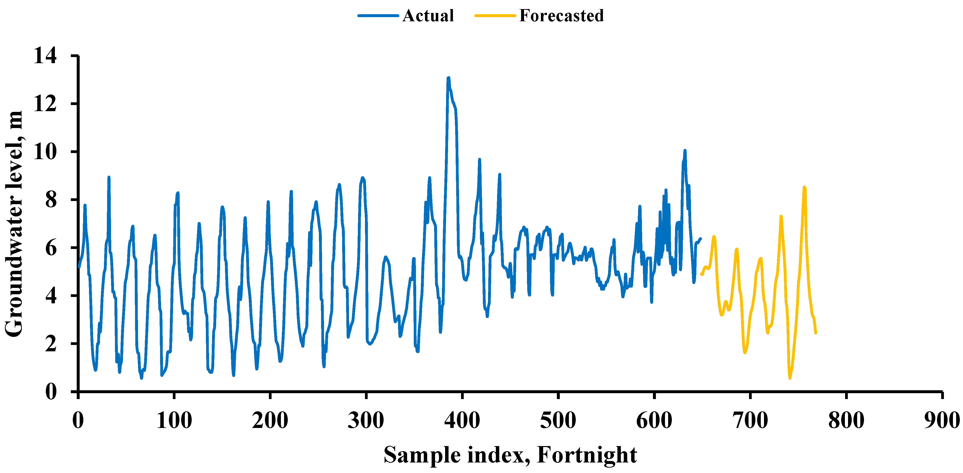
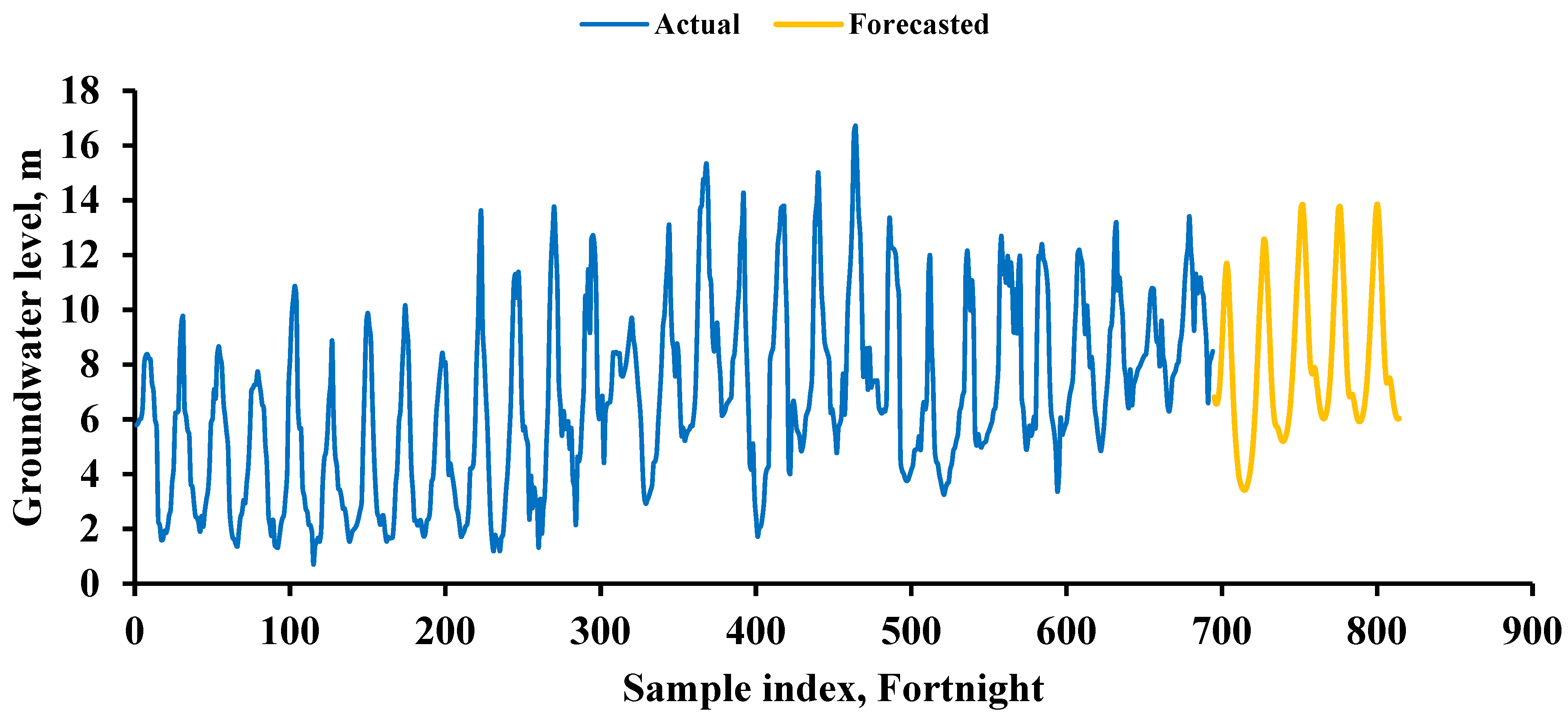
1. Introduction

Groundwater has become a cornerstone of global water security, sustaining agricultural production, domestic supply, ecosystem services, and economic activities. In many regions where surface water resources are insufficient or unreliable, groundwater acts as a critical buffer that supports human and environmental needs. However, unlike surface water, groundwater systems, particularly intergranular and fractured aquifers, are generally characterized by slow recharge processes, making them inherently vulnerable to overexploitation, whereas karst aquifers may exhibit much faster and more heterogeneous recharge behavior due to their unique hydrogeological structure. As a result, the sustainable management of subsurface water resources has become a central challenge for long-term development [1]. Increasing anthropogenic pressures including climate change, urban expansion, agricultural intensification, industrial growth, and population increase have significantly elevated groundwater demand worldwide [2,3]. Additional stressors such as unregulated abstraction, land-use transformations, and inefficient water use practices have further intensified depletion risks [4]. Consequently, groundwater resources are finite and increasingly strained across many parts of the world [1], with particularly acute implications for water-scarce regions such as northwestern Bangladesh.

The northwestern region of Bangladesh, especially the “Barind Tract”, is widely recognized for its susceptibility to water scarcity due to its semi-arid climatic conditions and challenging hydrogeological characteristics. Groundwater plays a dominant role in meeting irrigation and domestic water demands in this region, where surface water availability is limited and highly seasonal. However, recent trends indicate that groundwater abstraction has surpassed natural recharge rates, largely driven by the rapid expansion of irrigated agriculture [5]. The ‘Barind Tract’, distinguished by elevated topography with undulating terrain (27–47 m above mean sea level), high drainage density, and inefficient rainwater retention, experiences significant surface runoff losses [5]. Hydrogeologically, the area is constrained by areas with low hydraulic permeability (57%) [6] and low infiltration rates (2–3 mm/d) due to the presence of ‘Pleistocene-aged Barind clay’ soils [7], which significantly restrict aquifer recharge potential [8,9]. These factors, combined with erratic rainfall, frequent droughts, and insufficient soil moisture, result in persistent water shortages, particularly during the dry and pre-monsoon seasons. In this context, groundwater, extracted primarily through shallow and deep tube wells, remains the principal source for irrigation and potable use [8].

Understanding and predicting groundwater level (GWL) fluctuations is therefore essential for effective water resource management in such vulnerable settings. GWL dynamics are integral to the hydrogeological cycle and influence a wide range of hydrological and environmental processes. Accurate forecasting of GWL trends enables better planning, allocation, and sustainable utilization of groundwater resources. Traditionally, numerical and empirical models have been employed to simulate groundwater behavior using physical principles and statistical relationships [10,11]. Numerical models, in particular, have been widely used to analyze aquifer systems and quantify groundwater resources [12]. However, these models often require extensive datasets, detailed parameterization, and significant computational effort, while also being constrained by simplifying assumptions regarding complex subsurface processes [13,14]. Empirical models, on the other hand, may struggle to capture the nonlinear and dynamic nature of groundwater systems, limiting their adaptability and predictive accuracy under changing conditions [15]. Despite decades of advancements, challenges remain in achieving reliable and efficient groundwater predictions, particularly in data-scarce environments. Accurate short- and medium-term forecasting of GWL is critical for adaptive water management, especially in regions experiencing intensive groundwater extraction or ecological sensitivity [16,17]. A major limitation in this regard is the lack of consistent, high-quality datasets, which hinders the performance of conventional modelling approaches. Therefore, developing robust and data-driven modelling frameworks capable of effectively capturing groundwater dynamics remains an urgent priority for sustainable water resource management.

Due to the inherently dynamic and stochastic nature of subsurface water systems, the development of credible and dependable predictive models is instrumental in effectively addressing associated challenges. Furthermore, compared with mathematical modelling techniques, Machine Learning (ML) approaches achieve higher accuracy; therefore, it is recommended that researchers adopt advanced ML techniques for predicting GWL changes [18]. In this context, recent advances in ML have demonstrated significant potential for capturing the time-varying and uncertain nature of subsurface hydrological systems [12]. In the past few years, ML has gained prominence as a leading approach for GWL predictions. For instance, ref. [19] provided a comparison of Random Forest (RF) and Support Vector Machine (SVM) with Simple Recurrent Neural Network (RNN) and Long Short-Term Memory (LSTM) models for simulating GWL variations in an aquifer system of South Africa. The study found that SVM provided the smallest Root Mean Squared Error (RMSE), while RF achieved the best results with regard to Mean Absolute Error (MAE). In another study, ref. [20] evaluated several ML approaches, including Multiple Linear Regression (MLR), Multivariate Adaptive Regression Splines (MARS), Artificial Neural Networks (ANN), RF, and Gradient Boosting Regression (GBR), and reported that GBR outperformed the other models. In a different investigation, ref. [21] investigated the capability of Group Method of Data Handling (GMDH), Bayesian Network (BN), and ANN to predict GWL in the Birjand aquifer, and reported that GMDH provided the most accurate results among the tested approaches. Previous studies have reported that commonly applied ML approaches include Decision Trees (DT) [4,19], Improved Reptile Search Algorithm-based ANN (IRSA-ANN) [20], Fuzzy Logic models [21,22], IRSA-ANFIS [20], Linear Regression (LR) [4], Gaussian Process Regression (GPR) [4,23], Non-Linear Autoregressive Network with Exogenous Inputs (NARX) [4,5], Prophet forecasting model [24,25,26], and Radial Basis Function (RBF) networks [27,28], and Nonlinear Autoregressive Exogenous Neural Network (NARX–NN) [29,30]. A comprehensive overview of ML techniques applied for GWL prediction can be found in [31] and is therefore not repeated here. Additionally, refs. [32,33] presented comprehensive reviews of ML-based models for GWL prediction. However, a substantial body of existing literature has already demonstrated the limitations of classical statistical and traditional ML approaches such as linear models, ARIMA-type models, and tree-based regressors in capturing the highly nonlinear, non-stationary, and complex temporal dynamics typically observed in groundwater systems [34,35,36].

Another line of research has demonstrated that cutting-edge approaches such as deep neural networks with multiple hidden layers have demonstrated strong strength in representing complicated and nonlinear associations in datasets (e.g., [37]), leading to improved accuracy in environmental prediction tasks. Deep learning (DL) models employ advanced computational algorithms to detect complex patterns that are often difficult to capture using traditional physics-based approaches, particularly in cases where the governing physical processes are highly complex, not fully understood, or when simplified physical models are insufficient [38]. Considering this context, DL algorithms have been broadly investigated and employed in classification and regression tasks together, providing an effective approach for GWL prediction [13]. As an example, ref. [39] investigated an LSTM model to predict GWL that has significant practical importance in groundwater management. In a related study, ref. [40] contrasted LSTM, Multilayer Perceptron (MLP), and Gated Recurrent Unit (GRU) models for GWL prediction and reported that the GRU outperformed the other approaches. Similarly, ref. [41] evaluated Graph Neural Networks (GNN), LSTM, and GRU for GWL projection in British Columbia, Canada, and reported that the GNN demonstrated superior overall performance relative to the other approaches. In another study, ref. [10] compared Convolutional Neural Networks (CNN) and LSTM models for the forecasting of GWLs and found that CNNs provided higher accuracy, whereas LSTM models performed better in multi-step forecasting simulations. In a subsequent study, ref. [22] compared CNN, RNN, and Generative Adversarial Network (GAN), and reported that the CNN technique achieved superior overall efficiency amongst all the methods considered. Ref. [42] developed MLP and LSTM models for GWL forecasting and reported that MLP performed better during the pre-monsoon period, whereas LSTM showed superior performance for post-monsoon predictions. Ref. [43] developed an LSTM-based neural network for GWL forecasting using only historical groundwater data as input, applied to the Edwards Aquifer in Texas. The findings showed that LSTM consistently surpassed a CNN model and provided accurate predictions across short- and long-term horizons, including forecasts from one up to 26 time steps ahead. These studies indicate that different modelling approaches perform better at different locations, highlighting that model efficiency is strongly driven by the characteristics of training data.

To improve predictive performance, recent studies have increasingly focused on hybrid modelling approaches, which have demonstrated strong potential in reducing the shortcomings of standalone models and in producing more robust and reliable predictions [44]. For instance, ref. [45] developed an integrated framework combining gradient boosting models (XGBoost and LightGBM) and neural network approaches (LSTM and MLP) with Basin Hopping Optimization (BHO) to enhance GWL forecasting accuracy and reported that the XGBoost–BHO model achieved the best overall performance. In a different study, ref. [46] proposed a novel hybrid DL framework, CNN-BP, which combines CNN with Backpropagation Neural Networks (BPNN) to predict GWLs up to three days ahead across several observation wells. The study established that the proposed hybrid model surpassed the standalone BPNN model. Similarly, ref. [47] proposed a hybrid CEEMDAN–GA–DBN model compounding data decomposition (CEEMDAN), feature selection (GA), and a Deep Belief Network (DBN), along with quantile regression for uncertainty analysis, to forecast one-, two-, and three months ahead GWLs in the Jiuquan Basin, China. The proposed model outperformed both the CEEMDAN–DBN hybrid and standalone DBN across all lead periods and monitoring locations. Later, ref. [48] developed a hybrid LSTM–Grey Wolf Optimization (GWO) model for GWL estimation and compared its performance with a GWO-optimized ANN (ANN–GWO) and a standalone ANN. The results show that the LSTM–GWO approach provided more accurate GWL predictions than both alternative models. Ref. [49] proposed a hybrid GWL forecasting framework, STL–IWOA–GRU, which integrates LOESS-based seasonal trend decomposition (STL), an Improved Whale Optimization Algorithm (IWOA), and a GRU model. The results indicate that the improved optimization strategy enhanced the rate of convergence and global exploration capability, improving overall model performance. Ref. [50] formulated a novel hybrid framework that integrates LSTM with Empirical Mode Decomposition (EMD) and Wavelet Transform (WT) to improve GWL predictions. The results indicate that the EMD–LSTM model delivers better results than both the Wavelet–LSTM and the conventional standalone LSTM, particularly in cases where prediction errors are primarily driven by underlying trend components. Ref. [51] developed a novel ensemble ML model that combines both shallow (RBF, ANFIS, ANN) and deep learning (RNN, LSTM, CNN) approaches, optimized using the Coronavirus Herd Immunity Optimizer (CHIO), for GWL prediction. Their results show that the suggested ensemble model surpassed all individual standalone models.

In a different study, ref. [52] proposed a hybrid LSTM–Lion Algorithm (LSTM–LA) model for GWL forecasting using historical groundwater and precipitation information from a monitoring well in Karnataka, India. The findings revealed that the fusion LSTM–LA model achieved better prediction precision than both standalone LSTM and Feedforward Neural Network (FFNN) models. Ref. [53] developed an Augmented Artificial Ecosystem Optimization-based Multi-Layer Perceptron (AAEO-MLP) for one-month-ahead GWL forecasting. When evaluated against 17 benchmark models, AAEO-MLP demonstrated superior accuracy, convergence, and stability, highlighting the effectiveness of AAEO as an optimization technique for ML models such as MLP. Ref. [54] introduced a multi-step modelling approach for GWL simulation that integrates WT with an LSTM network (WT-MLSTM). Comparative analysis with a SVM model showed that the proposed hybrid framework provides superior performance. Ref. [55] developed a DL framework for GWL prediction that remains effective even with limited data. Their hybrid CNN–LSTM–ML model combines convolutional and LSTM networks to capture temporal relationships between GWLs and meteorological variables, while a meta-learning strategy enhances performance under data-scarce conditions. The results indicate that this model surpasses other approaches in both short-duration (one-month) and long-duration (twelve months) settings forecasting accuracy. Ref. [56], in a review of multiple studies, highlighted that DL models such as LSTM and CNN substantially enhance prediction accuracy across various temporal and spatial scales. They further emphasized that coupling these models with optimization techniques improves reliability. Consequently, hybrid approaches tailored to specific hydrological and hydrogeological settings can significantly strengthen GWL prediction and support more effective water resources management. Given the promise of DL and hybrid models in earlier studies, this research aims to develop standalone and hybrid GRU and LSTM models, along with optimized GRU and LSTM models using Genetic Algorithm (GA) and Particle Swarm Optimization (PSO).

Another notable concern is that model evaluation in groundwater studies often yields inconsistent outcomes when different statistical metrics are applied. A model that performs well in terms of Correlation Coefficient (R) may not necessarily demonstrate superior performance when assessed using error-based measures such as RMSE. For instance, ref. [19] reported that in GWL prediction, the SVM model achieved the lowest RMSE, while the RF model performed best in terms of MAE, highlighting inconsistencies in model ranking across different evaluation metrics. Such inconsistencies make it difficult to identify a single best-performing model based on any individual criterion. Therefore, a comprehensive assessment framework that incorporates multiple performance indicators is essential for robust model selection. In this regard, multi-criteria decision-making approaches provide a systematic means of integrating diverse evaluation metrics. Among these, Shannon’s Entropy (SE) method [57,58] has been widely adopted to determine the contribution level (weights) of various performance indices [59]. In addition, the CRITIC (Criteria Importance Through Intercriteria Correlation) technique introduced by [60] is an “objective weighting” technique that determines the importance of criteria grounded in both their variability (standard deviation) and the level of criterion conflict based on correlation. Another effective technique is the Evaluation based on Distance from Average Solution (EDAS), proposed by [61], which has demonstrated strong applicability in addressing multiple-criteria decision-making issues [62]. By combining CRITIC and EDAS, a more balanced and objective model ranking framework can be established. In this study, CRITIC is employed to compute the weights of selected evaluation criteria, while EDAS utilizes these weights to rank competing models, thereby enabling a more reliable identification of the most suitable model for GWL prediction.

In addition, a key overarching issue is that despite the widespread application of ML and DL techniques for simulating GWL variations across diverse hydrogeological settings, relatively limited attention has been given to forecasting beyond the range of existing historical observations. For example, ref. [63] applied a state-space approach in continuous time to estimate GWL at designated observation wells in Bangladesh and demonstrated its capability to reproduce historical trends while extending predictions beyond the training period. In another study, ref. [31] provided projections of GWL oscillations in an aridity-affected area of Bangladesh by comparing DL and dynamic system response models, including LSTM, ARMA, and state-space approaches, to support improved water resources management and long-term planning. They reported only the performance results of the LSTM-based DL models. Similarly, ref. [4] implemented a NARX model to generate forecasts up to one year ahead, reporting satisfactory predictive performance. Nonetheless, the trained models used in their projections remained limited. These gaps highlight the need for developing more advanced modelling frameworks capable of producing longer-term GWL forecasts while enabling rigorous comparison among different modelling strategies.

In response to these limitations, the present study explores the application of advanced DL and hybrid modelling approaches, including LSTM networks, GRU, Hybrid LSTM-GRU, and optimization algorithm-tuned GRU and LSTM models, for GWL projections in an aridity-prone area of Bangladesh. The performance of the developed models was evaluated against that of the well-established univariate time-series forecasting model ARIMA. The models primarily learn temporal correlations embedded within historical groundwater observations. The principal objective of this study is to evaluate the capability of standalone, hybrid, and optimization-based DL frameworks for data-driven GWL forecasting in a drought-affected and data-limited region where long-term and spatially consistent hydro-meteorological, abstraction, and recharge datasets are limited or unavailable. In many practical groundwater management situations in developing regions, reliable continuous records of pumping rates, recharge fluxes, irrigation withdrawals, and aquifer properties are often not accessible. Under such constraints, time-series-based DL approaches provide a practical alternative for capturing temporal groundwater fluctuations and generating future projections. Through systematically juxtaposing these techniques and identifying the most effective models, the research intends to establish a reliable predictive framework for groundwater planning and decision-making. As far as the authors are aware, the integration of these modelling techniques for long-term GWL projection has not been previously investigated in this region. Therefore, the particular aims of this research are: (i) to develop DL and hybrid DL-based models for simulating GWL fluctuations; (ii) to evaluate and rank model performance using a CRITIC–EDAS-based multi-criteria decision framework incorporating multiple statistical indicators; and (iii) to apply the top-performing DL models at individual monitoring locations to generate impending GWL projections, thereby supporting informed groundwater planning and decision-making. It is noted that the proposed framework is intended to support groundwater planning and decision-making rather than provide a complete groundwater management solution. The novelty of the study does not claim the invention of a completely new algorithm. Rather, it stems from: (i) the development and comparison of multiple standalone, hybrid, and metaheuristic-optimized DL frameworks under a consistent modelling environment; (ii) the incorporation of a CRITIC–EDAS-based multi-criteria ranking framework to address inconsistencies associated with single-metric model evaluation; and (iii) the implementation of recursive long-term GWL projection beyond the available observation period.

The remainder of this paper is structured as follows. Section 2 presents the methodology, including the description of the study area and dataset (Section 2.1), the standalone DL models, hybrid architectures, and optimization algorithm-tuned DL models employed in this study (Section 2.2), model configurations and tunable parameters (Section 2.3), model training and hyperparameter optimization procedures (Section 2.4), computational time analysis (Section 2.5), model performance evaluation metrics (Section 2.6), and the framework for identifying the best-performing model (Section 2.7). Section 3 presents experimental results and comparative evaluation of model performance across different observation wells. Section 4 discusses the implications of the findings for sustainable groundwater management. Finally, Section 5 summarizes the major conclusions of the study and Section 6 highlights future research directions.

2. Methodology

2.1. Study Area and Dataset Overview

The study region lies in the Rajshahi District of the Rajshahi Division in northwestern Bangladesh, encompassing approximately 2425.37 km². Geographically, the region extends between latitudes 24°07′ N to 24°43′ N and longitudes 88°17′ E to 88°58′ E. This area is largely part of the ‘Barind Tract’, a distinctive geomorphological unit characterized by elevated, dome-shaped undulating terrain ranging from 27 to 47 m above mean sea level. The uneven terrain and relatively dense fluvial network limit effective rainwater retention, causing substantial surface runoff that ultimately drains into major river systems [5]. Underground water constitutes the principal supply of irrigation water in this area and is extensively extracted through both shallow and deep groundwater boreholes [8]. Nonetheless, the hydrogeological conditions are constrained by a significant proportion (approximately 58%) of low to very low groundwater potential associated with poor hydraulic properties [6]. In addition, the presence of ‘Pleistocene-aged Barind clay’ as the dominant topsoil layer results in very low infiltration rates (2–3 mm/day), thereby limiting natural recharge processes [7,8,9].

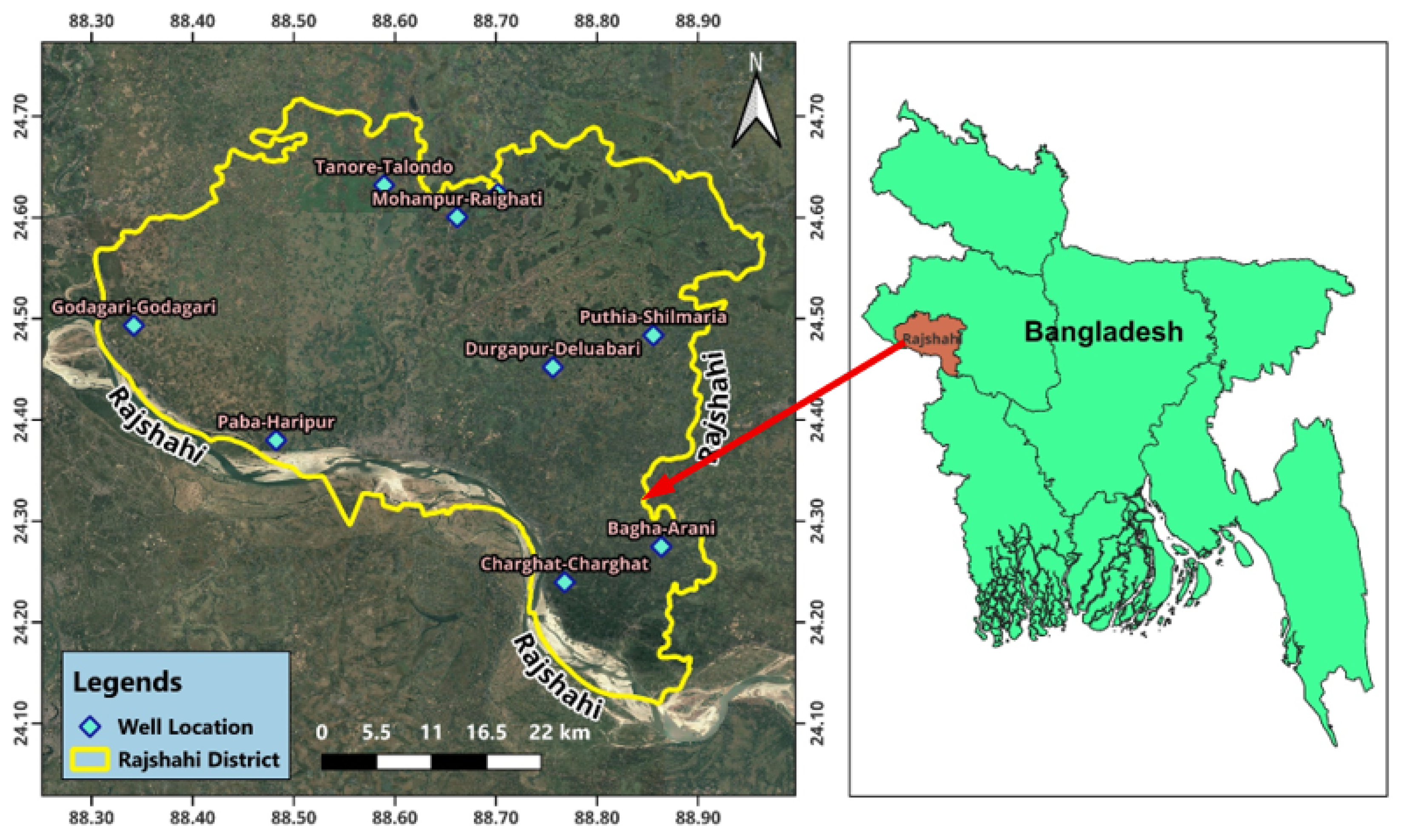
For this research, time-series data of GWLs were collected from nine observation bores distributed across nine upazilas (sub-districts) within the study region. Figure 1 presents the spatial distribution of the study area, highlighting the locations of the observation wells used in the analysis.

The following paragraphs describe the data sources, preprocessing procedures, and modelling framework adopted for analyzing GWL dynamics and generating future projections. Historical GWL records were used to develop predictive models and simulate future conditions at selected observation wells, with the objective of producing five-year forecasts. The dataset consists of fortnightly GWL measurements obtained from the Barind Multipurpose Development Authority (BMDA). BMDA is responsible for regional water resource management and operates approximately 8728 groundwater boreholes, each having a flow rate of two cusecs [64]. The dataset comprises manually recorded measurements representing the depth of groundwater below the land surface. A rigorous screening process was applied to the available datasets, and nine observation wells distributed across nine upazilas in the Rajshahi district were selected based on the criterion of minimal missing data. To enhance data reliability and ensure consistency in model development, a comprehensive data quality control procedure was implemented. This included range and limit checks to verify that all observations fell within physically plausible bounds, with any values outside the acceptable range treated as invalid. Only validated data points were utilized for subsequent modelling and long-term projections.

Although a small proportion of missing data (approximately 0.35–0.60%) was identified, these gaps were filled employing the Piecewise Cubic Hermite Interpolating Polynomial technique [65], which preserves the shape and monotonicity of the data. Outliers were detected and addressed through the Generalized Extreme Studentized Deviate test [66]. Following data cleaning and preprocessing, descriptive statistical analysis was conducted, as summarized in

Table 1. Statistical characteristics of groundwater level (GWL) data (m above mean sea level) at the selected observation wells.

Observation Well	Mean	STD	Skewness	Kurtosis
Bagha–Arani	4.571	1.545	0.488	0.058
Bagmara–Auchpara	10.210	5.447	0.576	−0.670
Charghat–Charghat	4.990	2.167	0.354	0.849
Durgapur–Deluabari	0.813	0.813	0.813	0.813
Godagari–Godagari	19.009	4.060	−0.579	−0.482
Mohanpur–Raighati	10.464	4.828	0.290	−0.721
Paba–Haripur	9.36	3.48	0.29	−0.40
Puthia–Shilmaria	5.15	3.09	0.55	−0.25
Tanore–Talondo	11.726	4.004	−0.268	−1.092

. The descriptive statistics of GWL data across the selected observation wells presented in Table 1 reveal substantial spatial variability in both magnitude and distributional characteristics.

The mean GWL values vary considerably among the wells, reflecting spatial differences in groundwater recharge conditions, aquifer properties, and the intensity of groundwater abstraction for irrigation. The lowest mean value at Durgapur–Deluabari (0.813 m) indicates persistently shallow groundwater conditions, likely influenced by strong local recharge from precipitation and surface water interaction. In contrast, the highest mean at Godagari–Godagari (19.009 m) suggests deeper water tables, which may be associated with lower recharge efficiency, higher abstraction demand, or less permeable aquifer materials limiting recharge. Other locations such as Tanore–Talondo (11.726 m), Mohanpur–Raighati (10.464 m), and Bagmara–Auchpara (10.210 m) also reflect relatively deeper groundwater conditions, potentially indicating moderate recharge rates combined with sustained groundwater pumping for irrigation. Conversely, Bagha–Arani (4.571 m) and Charghat–Charghat (4.990 m) exhibit comparatively shallow groundwater levels, likely supported by higher recharge contribution from rainfall and proximity to surface water bodies.

The standard deviation values represent temporal variability in groundwater levels, which is strongly influenced by seasonal precipitation recharge and groundwater extraction for irrigation. The highest variability was observed at Bagmara–Auchpara (5.447 m), followed by Mohanpur–Raighati (4.828 m) and Godagari–Godagari (4.060 m), suggesting strong seasonal fluctuations driven by alternating monsoon recharge and dry-season pumping stress. In contrast, Durgapur–Deluabari (0.813 m) shows relatively stable conditions, likely due to consistent recharge inputs and/or hydraulic buffering effects of local hydrogeological settings. Moderate variability at wells such as Paba–Haripur (3.48 m) and Puthia–Shilmaria (3.09 m) indicates balanced recharge–discharge dynamics.

The skewness values provide additional insight into how episodic hydrological processes such as intense rainfall events or seasonal pumping influence groundwater dynamics. Positive skewness in wells such as Bagha–Arani (0.488), Bagmara–Auchpara (0.576), and Puthia–Shilmaria (0.55) indicates occasional high groundwater levels likely resulting from strong recharge events. The pronounced positive skewness at Durgapur–Deluabari suggests frequent shallow conditions with occasional recharge-driven peaks. In contrast, negative skewness at Godagari–Godagari (−0.579) and Tanore–Talondo (−0.268) may reflect sustained groundwater abstraction and delayed or limited recharge response, resulting in more frequent lower water level occurrences.

The kurtosis values describe the influence of extreme hydrological events on groundwater variability. Negative kurtosis in wells such as Bagmara–Auchpara (−0.670), Mohanpur–Raighati (−0.721), and Tanore–Talondo (−1.092) indicates relatively dampened responses to extreme recharge or pumping events, suggesting more buffered aquifer systems. Conversely, positive kurtosis at Charghat–Charghat (0.849) and Durgapur–Deluabari (0.813) reflects greater sensitivity to extreme hydrological conditions, such as episodic heavy rainfall recharge or intensive short-term pumping. Bagha–Arani (0.058) approximates a normal distribution, indicating relatively balanced recharge and discharge conditions over time.

Overall, Table 1 highlights substantial spatial heterogeneity in groundwater level dynamics, governed by the interplay of precipitation-driven recharge, irrigation-induced abstraction, and site-specific hydrogeological characteristics. These processes collectively explain the observed variations in central tendency, variability, and distribution shape, underscoring the need for location-specific modelling approaches for reliable groundwater prediction and sustainable management.

2.2. Deep Learning Models

Before describing LSTM and GRU models, it is important to first outline the structure of the RNN, as both are extensions of this basic framework. An RNN is composed of repeating modules that share the same structure across time steps. Its output at any given time depends not only on the current input but also on information carried from the previous hidden state [67]. In principle, RNNs can utilize information from long input sequences; however, in practice, their performance is limited by vanishing and exploding gradient issues, particularly for long sequences. To overcome these limitations, more advanced architectures such as LSTM and GRU were introduced [68].

2.2.1. Long Short-Term Memory (LSTM) Networks

LSTM networks are an advanced form of RNNs specifically developed to model and retain long-range dependencies within sequential data [69]. LSTM models incorporate a specialized internal structure with gating mechanisms that regulate the flow of information through the network. LSTM networks share a sequential chain structure similar to traditional RNNs, but their internal architecture is more sophisticated, enabling them to learn temporal dependencies at both short and long scales. In contrast to standard RNNs, LSTMs incorporate an additional cell state that acts as a memory component for storing information over time. This memory is governed by three gates: the “forget gate”, “input gate”, and “output gate”. These gates function as filters that control information flow [70]: the forget gate removes irrelevant information from the cell state, the input gate governs the addition of new information, and the output gate controls the portion of the cell state that is passed forward to the next layer as output. Through this gating system, LSTM networks are able to effectively capture complex temporal relationships, offering a significant improvement over conventional RNNs [67].

The LSTM architecture is a complex neural network design that is specifically engineered to effectively store, control, and transmit information across long input sequences. Its improved capability arises from multiple interconnected components that work together to regulate information flow and maintain relevant temporal dependencies:

(i)

Cell State ($C_t$): The cell state functions as the internal memory component of the LSTM network, responsible for preserving and transmitting relevant information across successive time steps. It is progressively updated throughout the sequence, enabling the model to retain important contextual information over long temporal horizons. This mechanism allows the LSTM to maintain past information with minimal degradation, thereby supporting effective long-term dependency learning.

(ii)

Hidden State ($h_t$): The hidden state represents the output generated by the LSTM at each time step (t) and is typically used for downstream prediction tasks. It aggregates and summarizes the information contained in the input sequence up to the current time step and is propagated forward to the next LSTM unit. Functionally, the hidden state can be viewed as a selectively filtered representation of the cell state, retaining only the most relevant features required for the current prediction. This adaptive behavior enables the model to continuously update its output based on the evolving temporal context of the input sequence.

(iii)

Gates: LSTM networks incorporate three gating mechanisms that regulate the flow of information through the network, with each gate serving a specific functional role:

Input Gate ($i_t$): The input gate controls the extent to which new information from the current input is allowed to update the cell state. It employs a sigmoid activation function to produce values in the range of 0 to 1, thereby acting as a selective filter that determines how much of the incoming information should be retained. The mathematical expression for the input gate is given as follows:

$$i_t=\sigma \left(W_i·\left[h_{t-1},x_t\right]+b_i\right)$$

(1)

Here, $i_t$ is the input gate activation, and $\sigma$ is the sigmoid activation function, which outputs values in the range (0, 1), $W_i$ is the weight matrix, $h_{t-1}$ is the hidden state from the previous time step, $x_t$ is the current input, and $b_i$ is the bias term.

Forget Gate ($f_t$): The forget gate is responsible for determining which information from the previous cell state should be retained or removed. It uses a sigmoid activation function to generate values between 0 and 1, where values close to 0 indicate that information should be discarded, and values close to 1 indicate that it should be preserved. The mathematical formulation of the forget gate is expressed as follows:

$$f_t=\sigma \left(W_f·\left[h_{t-1},x_t\right]+b_f\right)$$

(2)

In this formula, $f_t$ is the forget gate activation, $W_f$ is the weight matrix, and $b_f$ is the bias term.

Output Gate ($o_t$): The output gate regulates the portion of the cell state that is exposed as the hidden state and passed to the next time step. It determines which information is relevant for producing the current output of the network. This gate also employs a sigmoid activation function to control the flow of information. The mathematical formulation of the output gate is given as follows:

$$o_t=\sigma \left(W_o·\left[h_{t-1},x_t\right]+b_o\right)$$

(3)

Here, $o_t$ is the output gate activation, $W_o$ is the weight matrix, and $b_o$ is the bias term.

The evolution of both the cell state and hidden state is determined through a set of coupled update equations that integrate the effects of the input, forget, and output gates. These equations define how new information is incorporated, irrelevant information is discarded, and the final output representation is produced at each time step. The corresponding mathematical expressions are given as follows:

$$\overline{C_t}=\tanh \left(W_C·\left[h_{t-1},x_t\right]+b_C\right)$$

(4)

Here, $\overline{C_t}$ represents the candidate values for the cell state, $W_C$ is the weight matrix, and $b_C$ is the bias term.

$$C_t=f_t\otimes C_{t-1}+i_t\otimes \overline{C_t}$$

(5)

Here, $C_t$ is the updated cell state, $C_{t-1}$ is the previous cell state, and $\otimes$ denotes element-wise multiplication.

$$h_t=o_t\otimes \mathrm{t}\mathrm{a}\mathrm{n}\mathrm{h}\left(C_t\right)$$

(6)

Here, $h_t$ is the updated hidden state.

A graphical representation of the LSTM network is available in the study by [71] and is therefore not reproduced here. Readers interested in a comprehensive description of LSTM architectures and their operational mechanisms are referred to [71].

2.2.2. Gated Recurrent Unit (GRU)

A GRU neural network is designed to capture long-term dependencies and model highly nonlinear temporal relationships, particularly when the dataset size is moderate. Structurally, GRU shares conceptual similarities with LSTM networks, as both are based on gated mechanisms that regulate information flow through sequential data. However, GRU adopts a more streamlined architecture, making it computationally more efficient and easier to train. Due to its simplified structure, it contains fewer parameters than LSTM, which reduces model complexity while maintaining strong predictive capability. This compact design allows GRU to learn effectively with faster convergence and improved computational efficiency compared with more complex recurrent architectures [72].

Originally introduced in 1997 for language modelling tasks, LSTM networks are widely recognized for their strong ability to capture long-term dependencies in sequential data [73]. However, their relatively complex architecture often leads to longer training times. To address this limitation, the GRU model was later proposed as a simplified variant of LSTM, designed to retain similar performance while reducing computational complexity and accelerating the training process [74]. The GRU is an RNN variant developed to mitigate “vanishing and exploding” gradient problems during training. Via its internal gating structure and streamlined memory design, it effectively models temporal dependencies in time-series data and exhibits strong generalization ability. Compared with LSTM, GRU integrates the cell state and gating operations into a more compact structure, allowing more efficient information flow with fewer parameters. As a result, it is easier and faster to train while still capturing long-term dependencies and nonlinear relationships, making it a practical alternative to LSTM, particularly for moderately sized datasets [72].

In contrast to LSTM, the GRU architecture does not employ a separate memory cell. Instead, it uses a single hidden state ($h_t$) to carry and update information across time steps. Moreover, the traditional input and forget gates are merged into a single update gate ($z$), while the reset gate ($r_t$) controls how much past information from $h_{t-1}$ is incorporated when forming the candidate activation. Through this simplified gating structure, the GRU updates its hidden representation using both the current input at time ($t$) and the previous hidden state at time ($t-1$), resulting in a more compact and computationally efficient formulation. The GRU mechanism is defined by the following set of equations [74]:

$$z_t=\sigma \left(W_z{x}_t+U_z{h}_{t-1}+b_z\right)$$

(7)

$$r_t=\sigma \left(W_r{x}_t+U_r{h}_{t-1}+b_r\right)$$

(8)

$$\widetilde{h_t}=\tanh \left(W\tilde{h}{x}_t+U\tilde{h}\left(r_t\times {\tilde{h}}_{t-1}\right)+b\tilde{h}\right)$$

(9)

$$h_t=\left(1-z_t\right)\times h_{t-1}+z_t\times \widetilde{h_t}$$

(10)

In these equations, $\mathrm{t}\mathrm{a}\mathrm{n}\mathrm{h}$ and $\sigma$ denote the hyperbolic tangent and logistic sigmoid activation functions, respectively. The symbol “×” represents element-wise multiplication, while $b$ refers to the bias vector. All associated weights and biases are learnable parameters that are optimized during the training process. Due to the use of the sigmoid function, the outputs of the gating mechanisms are constrained within the range (0,1), enabling them to act as adaptive information filters. When the reset gate ($r_t$) is effectively closed (i.e., close to zero), the model relies primarily on the current input ($x_t$), whereas the update gate ($z_t$) regulates how much information from the previous hidden state ($h_{t-1}$) is retained and carried forward into the new hidden state ($h_t$).

Graphical representations of the GRU network are presented in [75] and are therefore not repeated here. Interested readers are referred to [75] for further details.

2.2.3. Genetic Algorithm-Tuned Gated Recurrent Unit (GA-GRU)

A GA–GRU model is developed to improve the accuracy of GWL time-series forecasting. The GRU network is an efficient RNN architecture designed to model nonlinear time-based reliance in time-series data by alleviating “vanishing gradient” issues through gating mechanisms [44]. However, the predictive performance of GRU models is highly sensitive to the selection of hyperparameters, the hidden layer size, learning rate, and training epochs. To address this limitation, a GA is employed in this study to optimize the GRU hyperparameters and enhance forecasting accuracy [76,77].

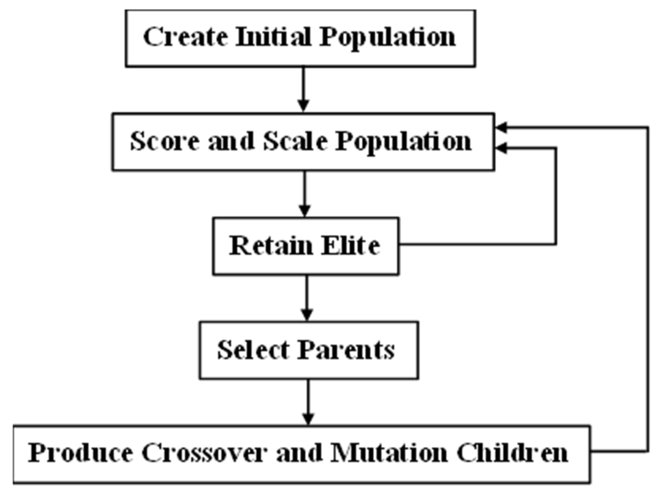
A GA is an optimization technique inspired by the principles of natural evolution and survival of the fittest. It is widely used to solve both constrained and unconstrained optimization problems. The algorithm begins with a population of candidate solutions and iteratively improves them through evolutionary operations such as selection, crossover, and mutation. During each iteration, individuals with better fitness are more likely to be chosen as parents to generate offspring for the subsequent generation. Through this evolutionary process, the population gradually converges toward an optimal or near-optimal solution. Genetic algorithms are particularly effective for complex optimization problems where traditional optimization approaches may perform poorly. These include problems characterized by discontinuous, nondifferentiable, stochastic, or highly nonlinear objective functions. In addition, GA can efficiently handle mixed-integer optimization problems in which certain decision variables are required to take integer values. The following flowchart (Figure 2) illustrates the principal steps of the proposed algorithm.

At each iteration, the genetic algorithm applies three primary operations to generate a new population from the existing set of candidate solutions. Selection: Selection operators identify the individuals, referred to as parents, that will contribute to the next generation. This process is typically probabilistic and is often influenced by the fitness values of the individuals. Crossover: Crossover operators create offspring by combining the characteristics of two parent solutions, thereby promoting the exchange of useful traits between individuals. Mutation: Mutation operators introduce random alterations to individual solutions, helping maintain population diversity and improving the algorithm’s ability to explore the search space.

In the GA–GRU framework, GA is used as a global optimization strategy to search for the optimal combination of GRU hyperparameters that minimizes the prediction error on training data. The optimization process recursively updates a “population of candidate solutions” using selection, crossover, and mutation operators until convergence. The GA is used to optimize the GRU hyperparameters by minimizing a predefined fitness function representing the prediction error. Each candidate solution (chromosome) consists of three decision variables: number of hidden GRU units, learning rate, and number of training epochs. The search space is defined within the following bounds: hidden units: 20–200, learning rate: ${10}^{-4}$ to ${10}^{-2}$, epochs: 100–1000. The GA evolves an initial “population of candidate solutions” using “selection”, “crossover”, and “mutation operators” over a fixed number of generations. In this study, a population size of 100 and a maximum of 1000 generations are used, with parallel computing enabled to enhance computational efficiency. The GA optimizes the GRU model by curtailing the Mean Squared Error (MSE) between the actual and predicted values. The objective function is defined as:

$$J(\theta )={\displaystyle \frac{1}{N}}{\displaystyle {\sum }_{i=1}^N}(y_i-{\widehat{y}}_i{)}^2$$

(11)

where $J\left(\theta \right)$ denotes the fitness function, $N$ is the total number of training samples, $y_i$ denotes the observed values, and ${\widehat{y}}_i$ quantifies the GRU-predicted outputs. The parameter vector $\theta$ corresponds to the GRU hyperparameters, i.e., number of units, learning rate, and epochs.

The optimal hyperparameter set is selected based on the smallest magnitude of the objective function, resulting in improved model generalization and forecasting performance. After convergence of the GA, the best-performing solution is extracted as: optimal number of GRU hidden units, optimal learning rate, and optimal number of epochs. These optimized parameters are subsequently used to train the final GA–GRU model for GWL prediction.

2.2.4. Genetic Algorithm-Tuned Long Short-Term Memory Networks (GA-LSTM)

In this study, a GA–LSTM model is developed to improve the accuracy of GWL forecasting. The LSTM network is a specialized RNN designed to capture both short- and long-term dependencies in sequential data through memory cells and gating mechanisms, including the input, forget, and output gates [73]. Despite its strong predictive capability, the effectiveness of LSTM models is greatly affected by hyperparameter settings including the number of hidden units, learning rate, and training epochs. To address this limitation, GA is employed as a global optimization technique to determine the optimal LSTM configuration [76,77]. The same hyperparameter optimization strategy and objective function formulation used in the GA–GRU model were also applied in this case. Specifically, the identical search space, including the number of hidden units, learning rate, and number of training epochs, was considered for tuning the model parameters. Similarly, the optimization process aimed to minimize the MSE-based objective function to evaluate model performance and guide the search for optimal solutions. This consistency ensures a fair comparison between different hybrid modelling approaches by maintaining uniform optimization criteria across all experiments.

After convergence of the GA, the best hyperparameter set was extracted and used to train the final GA–LSTM model. The optimized parameters include the optimal number of LSTM hidden units, the optimal learning rate, and the optimal number of training epochs. These optimized parameters were subsequently used to train the final GA–LSTM model for GWL prediction.

2.2.5. Hybrid Long Short-Term Memory-Gated Recurrent Unit (LSTM-GRU)

In this study, a hybrid LSTM–GRU model is developed to enhance the precision of GWL forecasts. The proposed architecture integrates the synergistic characteristics of LSTM and GRU networks to better capture complex temporal dependencies in sequential data. LSTM networks are effective in learning long-term dependencies through gated memory cells, while GRU networks provide a simplified gating mechanism that reduces computational complexity while preserving strong sequence learning capability [73,74]. By combining these two architectures in a single framework, the hybrid model leverages the feature learning capability of LSTM and the efficient time-based refinement capability of GRU.

The developed hybrid LSTM–GRU structure is implemented using the following steps: (a) A sequence input layer serves to accept univariate time-series data, (b) An LSTM layer with 128 hidden units is applied to extract high-level temporal features from the input sequence, (c) A GRU layer with 64 hidden units is used to refine and further learn temporal dependencies from the LSTM output, (d) A fully connected layer links the extracted feature representation to the output space, and (e) A regression layer is used for continuous value prediction. In the proposed framework, the LSTM layer first processes the input sequence and captures long-term temporal dependencies by maintaining internal memory states. The resulting feature sequence is then passed to the GRU layer, which further processes and refines temporal representations using its efficient gating mechanism. This sequential hybridization allows the model to benefit from both deep memory retention (LSTM) and computational efficiency (GRU), improving the ability to model nonlinear and non-stationary time-series dynamics. The fully connected layer transforms the learned features into the final prediction output, while the regression layer computes the loss for continuous variable estimation. The model is trained using backpropagation through time, minimizing the prediction error between observed and simulated values.

A graphical representation of the hybrid LSTM–GRU architecture is available in [78] and is therefore not reproduced in this study. Readers seeking a detailed visual illustration of the hybrid model are referred to [78].

2.2.6. Particle Swarm Optimization-Tuned Gated Recurrent Unit (PSO-GRU)

PSO is a population-based optimization technique in which a group of candidate solutions, referred to as particles, explores the search space by moving in iterative steps. At each iteration, the objective function is evaluated for every particle, after which their velocities and positions are updated based on the best solutions found. The method is inspired by the collective behavior of swarms such as flocks of birds or schools of fish. Each particle adjusts its movement by considering both its own best-known position and the best-known position discovered by the entire swarm. Through this collaborative search process, the particles gradually converge toward one or more promising regions of the solution space. Since PSO operates on a population of solutions rather than a single point, it shares conceptual similarities with genetic algorithms in terms of population-based global search.

At iteration $n$, each particle in the swarm is characterized by a velocity $v\left(n\right)$, which is influenced by three key components: its own best-known position $s\left(n\right)$, the best position identified within its neighborhood $g\left(n\right)$, and its previous velocity $v(n-1)$.

The particle position is then updated using the relation:

$$x(n+1)=x\left(n\right)+v\left(n\right),$$

(12)

with appropriate constraints applied to ensure that the updated position remains within the defined search boundaries.

The velocity update is typically expressed as:

$$v(n+1)=W\left(n\right)v\left(n\right)+r_1\left(s\right(n)-x(n\left)\right)+r_2\left(g\right(n)-x(n\left)\right),$$

(13)

where $r_1$ and $r_2$ are randomly generated scalar values in the interval $\left[0,1\right]$, and $W\left(n\right)$ denotes an inertia weight that may vary over iterations to balance exploration and exploitation.

In practice, the algorithm may incorporate dynamic neighborhood structures and additional adjustments when improved solutions are encountered, further enhancing its global search capability.

A PSO–GRU model is developed to enhance the predictive accuracy of time-series forecasting. GRU performance is highly dependent on hyperparameter configuration, particularly the number of hidden units, learning rate, and number of training epochs. Therefore, PSO is employed as a population-based global optimization technique to identify the optimal GRU hyperparameters [79]. In the PSO framework, each particle represents a candidate GRU configuration defined by three decision variables: number of hidden GRU units, learning rate, and number of training epochs. The search space is defined as: hidden units: 20–200, learning rate: ${10}^{-4}$ to ${10}^{-2}$, epochs: 100–1000. Each particle has a position and velocity that are progressively refined using each particle’s personal best and the global best solution of the swarm. The optimization is performed using a swarm size of 100 particles over 1000 iterations. A similar fitness function as in the case of GA-GRU was employed for the PSO-GRU model.

The PSO algorithm begins by initializing a particle population randomly within the defined bounds. Each particle’s initial velocity is set to zero, and its cost is evaluated using the GRU objective function. The personal best and global best positions are then identified. During each iteration, particle velocities are updated using “inertia weight” ($w=0.7$), “cognitive coefficient” ($c_1=1.5$), “social coefficient” ($c_2=1.5$). The velocity and position updates follow the standard PSO updating mechanism, and boundary constraints are enforced to ensure feasibility of solutions. After updating positions, the GRU model is retrained and evaluated to compute the new fitness values. The best solution is selected based on the minimum MSE achieved across all particles and iterations. The final outputs of the PSO optimization include optimal number of GRU hidden units, optimal learning rate, and optimal number of training epochs. These optimized parameters are then used to train the final PSO–GRU model for GWL prediction.

Details of the PSO implementation are provided in [34] and are therefore not repeated in this work. Readers are referred to [34] for a detailed description of the implementation.

2.2.7. Particle Swarm Optimization-Tuned Long Short-Term Memory Networks (PSO-LSTM)

A PSO–LSTM model is developed to improve the predictive performance of GWL forecasting. PSO is employed to optimally tune the hyperparameters instead of a GA [49]. Similar hyperparameters and objective function as in the case of the GA-LSTM were employed to tune the optimal LSTM parameters. The same hyperparameter set and objective function used in the PSO–GRU framework were also adopted for optimizing the LSTM model. Specifically, the LSTM architecture was tuned using identical decision variables, including the number of hidden units, learning rate, and training epochs, while the same error-based objective function was used to evaluate model performance. This ensures consistency in the optimization process and allows a fair comparison between the PSO–GRU and PSO–LSTM models under identical evaluation criteria. These optimized parameters are then used to train the final PSO–LSTM model, improving its generalization capability and forecasting accuracy for time-series applications such as GWL prediction.

The incorporation of GA and PSO in this study is not intended to introduce methodological novelty in the optimization algorithms themselves. Rather, the primary objective is to systematically examine whether metaheuristic-based hyperparameter tuning can enhance the predictive accuracy, stability, and robustness of DL models for GWL forecasting when compared with their corresponding non-optimized configurations. By employing GA and PSO as complementary search strategies, the study evaluates the extent to which automated hyperparameter optimization can improve model generalization across spatially heterogeneous and data-limited hydrogeological settings.

The proposed models were benchmarked against ARIMA, a widely recognized univariate time-series forecasting model. Given that ARIMA is a well established and extensively documented approach in scientific literature, a detailed description of the model is not provided in this study; instead, interested readers are referred to relevant published research for comprehensive methodological details.

2.3. Model Architecture and Tunable Parameters

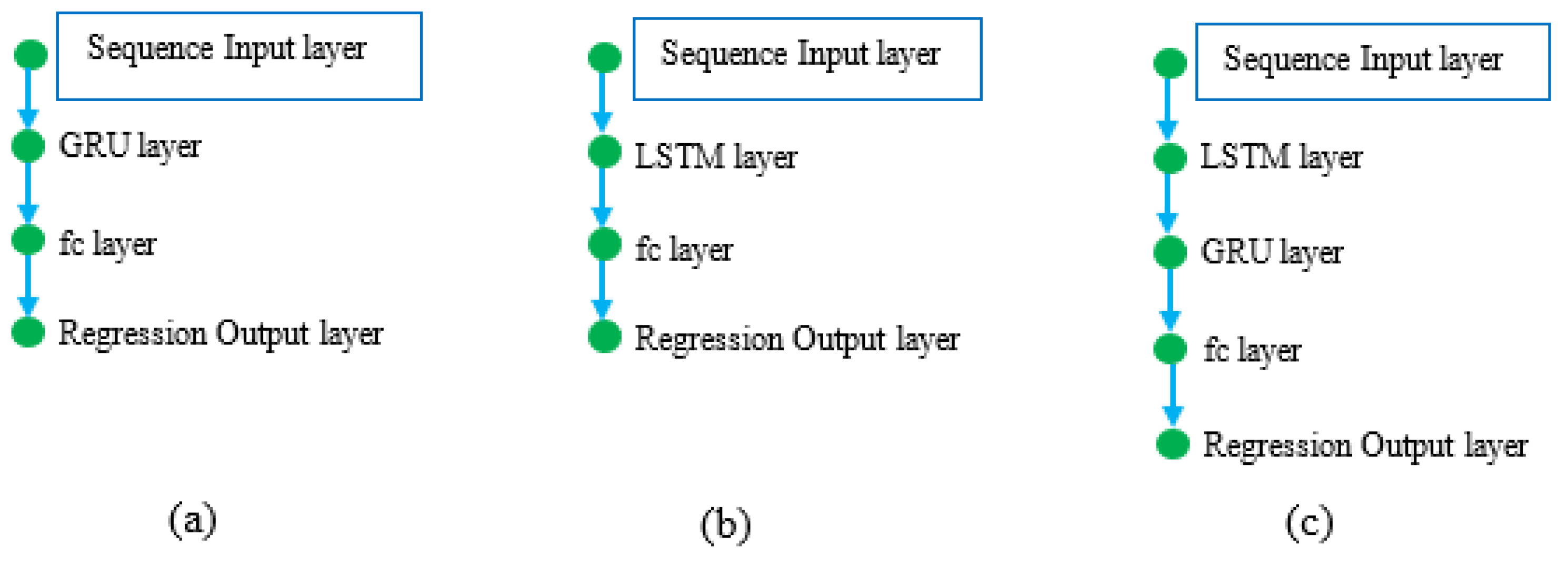
The GRU-based models were constructed using a sequential architecture designed to process the univariate GWL time series, with an input dimension of one corresponding to the single-variable nature of the dataset. The network consisted of an input layer, followed by a GRU layer, and a fully connected output layer with one neuron to generate the final prediction. Similarly, the LSTM models followed an analogous architecture, where the input layer accepted the univariate GWL series (input size = 1), followed by an LSTM layer and a dense output layer consisting of one neuron.

For the hybrid GRU–LSTM framework, a stacked architecture was implemented in which the input sequence was first processed through an LSTM layer, followed by a GRU layer, and finally a fully connected output layer with one neuron. This hybrid design aims to harness the synergistic strengths of both recurrent units in capturing temporal dependencies at different scales. In the case of the GA- and PSO-optimized GRU and LSTM models, the same baseline architectures were retained. Model architectures for the GRU, LSTM, and hybrid GRU-LSTM are illustrated in Figure 3.

The subsequent sections provide a thorough description of the network architectures developed for the Bagha–Arani station, including layer-wise configurations and the total number of trainable (learnable) parameters associated with each model. These details offer insights into the structural complexity and capacity of the implemented models. It is important to note that certain architectural attributes such as activation functions, the number of learnable parameters, and state dimensions vary across models developed for other observation wells. These variations arise due to differences in data characteristics and the outcomes of model-specific tuning procedures. For clarity and consistency in presentation, this section focuses exclusively on the configurations corresponding to the Bagha–Arani station. The reported parameters are therefore intended to serve as a representative example of the model structures employed in this effort.

The model layer information of the standalone GRU, LSTM, and hybrid GRU-LSTM are presented in

Table 2. Layer information of the GRU model developed at Bagha–Arani station (Total learnable parameters are 50,000).

Layer Number	Layer Name	Layer Type	Activations	Learnable Sizes	State Sizes
1	‘sequenceinput’ (Sequence input with 1 dimension	Sequence Input	1 (C) × 1 (B) × 1 (T)	-
2	‘gru’ (GRU with 128 hidden units)	GRU	128 (C) × 1 (B) × 1 (T)	Input Weights: 384 × 1 Recurrent Weights: 384 × 128 Bias: 384 × 1	Hidden State: 128 × 1
3	‘fc’ (1 fully connected layer)	Fully Connected	1 (C) × 1 (B) × 1 (T)	Weights: 1 × 128 Bias: 1 × 1	-
4	‘regressionoutput’ (mean-squared-error with response ‘Response’)	Regression Output	1 (C) × 1 (B) × 1 (T)	-	-

,

Table 3. Layer information of the LSTM model developed at Bagha–Arani station (Total learnable parameters are 66,600).

Layer Number	Layer Name	Layer Type	Activations	Learnable Sizes	State Sizes
1	‘sequenceinput’ (Sequence input with 1 dimension	Sequence Input	1 (C) × 1 (B) × 1 (T)	-
2	‘lstm’ (LSTM with 128 hidden units)	LSTM	128 (C) × 1 (B) × 1 (T)	Input Weights: 512 × 1 Recurrent Weights: 512 × 128 Bias: 512 × 1	Hidden State: 128 × 1 Cell State: 128 × 1
3	‘fc’ (1 fully connected layer)	Fully Connected	1 (C) × 1 (B) × 1 (T)	Weights: 1 × 128 Bias: 1 × 1	-
4	‘regressionoutput’ (mean-squared-error with response ‘Response’)	Regression Output	1 (C) × 1 (B) × 1 (T)	-	-

and

Table 4. Layer information of the GRU-LSTM model developed at Bagha–Arani station (Total learnable parameters are 1,03,600).

Layer Number	Layer Name	Layer Type	Activations	Learnable Sizes	State Sizes
1	‘sequenceinput’ (Sequence input with 1 dimension	Sequence Input	1 (C) × 1 (B) × 1 (T)	-	-
2	‘lstm’ (LSTM with 128 hidden units)	LSTM	128 (C) × 1 (B) × 1 (T)	Input Weights: 512 × 1 Recurrent Weights: 512 × 128 Bias: 512 × 1	Hidden State: 128 × 1 Cell State: 128 × 1
3	‘gru’ (GRU with 64 hidden units)	GRU	64 (C) × 1 (B) × 1 (T)	Input Weights: 192 × 128 Recurrent Weights: 192 × 64 Bias: 192 × 1	Hidden State: 64 × 1
4	‘fc’ (1 fully connected layer)	Fully Connected	1 (C) × 1 (B) × 1 (T)	Weights: 1 × 64 Bias: 1 × 1	-
5	‘regressionoutput’ (mean-squared-error with response ‘Response’)	Regression Output	1 (C) × 1 (B) × 1 (T)	-	-

. The model layer information of the GA- and PSO-tuned GRU and LSTM models are presented in Supplementary Information (Tables S1–S4). Table 2 presents the layer information of the developed GRU model.

The GRU model developed for the Bagha–Arani station is a compact yet effective DL architecture designed for sequence-based regression tasks. It consists of four layers with a total of approximately 50,000 learnable parameters, indicating a moderately complex network able to identify temporal dependencies in the dataset. The first layer is a sequence input layer, which accepts a univariate time-series input. The activation size of 1 (C) × 1 (B) × 1 (T) indicates that the model processes one feature (channel), one observation per batch, and one time step at a time. This structure is suitable for sequential environmental or hydrological data where each time step contains a single variable. The second layer is a GRU layer with 128 hidden units, which forms the core of the model. This layer maps the input to a higher-dimensional feature space with an activation size of 128 × 1 × 1, facilitating the model’s learning of complex temporal patterns. The GRU layer includes three sets of parameters corresponding to its gating mechanisms: (a) Input weights of size 384 × 1, (b) Recurrent weights of size 384 × 128, and (c) Bias vectors of size 384 × 1.

These dimensions arise because a GRU has three gates (update, reset, and candidate), each contributing 128 units (i.e., 3 × 128 = 384). The hidden state size of 128 × 1 represents the memory retained through successive time steps, facilitating the capture of both short-range and long-range dependencies efficiently. The third layer is a fully connected (dense) layer, which maps the 128-dimensional output of the GRU layer to a single output value. The activation size is reduced to 1 × 1 × 1, corresponding to a scalar prediction. This layer contains 128 weights (1 × 128) and a single bias term, effectively performing a linear transformation of the extracted embeddings. The terminal network layer is a regression output layer, which determines the loss using the MSE between the model-predicted and observed values. This layer does not contain learnable parameters and serves as the objective function for training the model. The GRU layer provides strong temporal feature extraction, while the fully connected and regression layers ensure accurate prediction of the target variable.

Table 3 presents the layer information of the standalone LSTM developed at the Bagha–Arani observation well. The LSTM developed for the Bagha–Arani site is a structured DL architecture designed to capture temporal dynamics in time-series data with enhanced memory capability. With a total of approximately 66,600 learnable parameters, the model is more complex than the GRU counterpart, primarily due to the additional gating mechanism and cell state in the LSTM unit.

The first layer is a sequence input layer, which accepts a univariate time-series input. The activation size of 1 (C) × 1 (B) × 1 (T) indicates that the model processes a single feature (channel), with one observation per batch and one time step at a time. This configuration is appropriate for sequential datasets such as hydrological or meteorological variables. The second layer is the LSTM layer with 128 hidden units, serving as the core component of the model. It produces an activation size of 128 × 1 × 1, transforming the input into a higher-dimensional feature space for learning temporal dependencies. The learnable parameters in this layer include: (a) Input weights of size 512 × 1, (b) Recurrent weights of size 512 × 128, and (c) Bias vectors of size 512 × 1.

These dimensions arise because the LSTM comprises four gates (input, forget, output, and candidate cell state), each with 128 units, resulting in 4 × 128 = 512 parameters per weight category. In addition to the hidden state (128 × 1), the LSTM maintains a cell state (128 × 1), which acts as a long-term memory pathway. This dual-state mechanism enables the LSTM to better preserve and regulate information over long sequences, reducing issues such as vanishing gradients and improving learning of long-term dependencies compared with simpler recurrent architectures. The third layer is a fully connected (dense) layer, which maps the 128-dimensional output from the LSTM layer to a single scalar output. The activation size becomes 1 × 1 × 1, representing the predicted value. This layer contains 128 weights (1 × 128) and a single bias term, performing a linear transformation of the extracted temporal features. The final layer is a regression output layer, which determines the loss using the MSE between predicted and observed values. This layer does not include learnable parameters and is used solely for model optimization during training. The LSTM architecture is well suited for complex time-series regression problems where long-term dependencies are significant. Its additional cell state and gating mechanisms provide improved memory retention and control over information flow, which explains the higher number of parameters and potentially enhanced predictive performance compared with the GRU model.

Table 4 presents the layer information of the hybrid GRU-LSTM developed for the Bagha–Arani observation well. The GRU–LSTM developed for the Bagha–Arani observation well represents a fusion DL structure that integrates the advantages offered by each LSTM and GRU models. With a total of approximately 103,600 learnable parameters, this model is more sophisticated than the individual GRU and LSTM networks, enabling improved learning of both immediate and extended temporal patterns in time-sequence data.

The first layer is a sequence input layer, which accepts a univariate time-series input. The activation size of 1 (C) × 1 (B) × 1 (T) indicates that the model processes a single feature at each time step, making it suitable for sequential environmental or hydrological datasets. The second layer is an LSTM layer with 128 hidden units, which serves as the initial temporal feature extractor. It transforms the input into a higher-dimensional representation with an activation size of 128 × 1 × 1. The learnable parameters include: (a) Input weights of size 512 × 1, (b) Recurrent weights of size 512 × 128, and (c) Bias vectors of size 512 × 1.

These dimensions arise from the four internal gates of the LSTM (input, forget, output, and candidate), each contributing 128 units. The layer maintains both a hidden state (128 × 1) and a cell state (128 × 1), allowing it to effectively capture long-term dependencies and retain important historical information. The third layer is a GRU layer with 64 hidden units, which further processes the features extracted by the LSTM layer. The activation size is reduced to 64 × 1 × 1, enabling dimensionality reduction while preserving essential temporal patterns. The learnable parameters of this layer include: (a) Input weights of size 192 × 128, (b) Recurrent weights of size 192 × 64, and (c) Bias vectors of size 192 × 1. These dimensions correspond to the three gates of the GRU (update, reset, and candidate), where 3 × 64 = 192. The hidden state size of 64 × 1 represents the compressed temporal representation passed to the next layer. The use of a GRU after the LSTM allows the model to refine and simplify the learned features, improving computational efficiency while maintaining predictive capability. The fourth layer is a fully connected (dense) layer, which maps the 64-dimensional output from the GRU layer to a single scalar output. The activation size becomes 1 × 1 × 1, corresponding to the final prediction. This layer contains 64 weights (1 × 64) and a single bias term, performing a linear transformation of the derived feature set. The final layer is a regression output layer, which determines the loss using the MSE between predicted and observed values. This layer has no learnable parameters and is used solely for model training and performance evaluation.

The GRU–LSTM hybrid architecture effectively combines long-range memory capability of LSTM with the computational efficiency and feature refinement of GRU. This layered design allows the model to first extract deep temporal features and then compresses and optimize them for accurate prediction, rendering it especially effective for complex time-series regression problems in hydrology and environmental modelling.

2.4. Model Training and Hyperparameter Tuning

For model development, the GWL data was partitioned into training and test subsets, with 90 percent of the observations allocated for training and the remaining 10 percent reserved for validation. Given the sequential and time-dependent structure of the dataset, random sampling was avoided to preserve temporal continuity. Although no universally accepted guideline exists for selecting an optimal data split ratio [80,81], the 90:10 division was ultimately adopted based on comparative trials that indicated improved model performance. This consistent partitioning strategy was applied across all models developed in this study to ensure comparability of results. The selection of a single hold-out split was guided by both methodological consistency and the practical constraints of limited hydrological time-series length at individual observation wells. In GWL forecasting studies, especially in data-scarce regions such as northwestern Bangladesh, maintaining sufficient training data is critical for DL models to effectively learn long-term temporal dependencies and nonlinear system behavior. The 90:10 split therefore represents a balance between maximizing training information while retaining an independent test set for unbiased evaluation. However, time-series model evaluation can be sensitive to the choice of the test period, and approaches such as rolling-origin or multiple temporal cross-validation can provide additional robustness. Nevertheless, in this study, the primary objective is comparative model assessment under a consistent experimental design rather than exhaustive uncertainty quantification across multiple temporal partitions. Applying a uniform hold-out strategy across all models ensures that performance differences are attributable to model structure and optimization rather than variations in training–testing configurations.

Prior to model training, both the training and test datasets were normalized using the z-score standardization technique. This transformation was performed employing the average ($\mu$) and standard deviation ($\sigma$) of the training data, as expressed by:

$${data}_s=\left(data-\mu \right)/\sigma$$

(14)

where $\mu$ denotes the mean value and $\sigma$ represents the corresponding standard deviation.

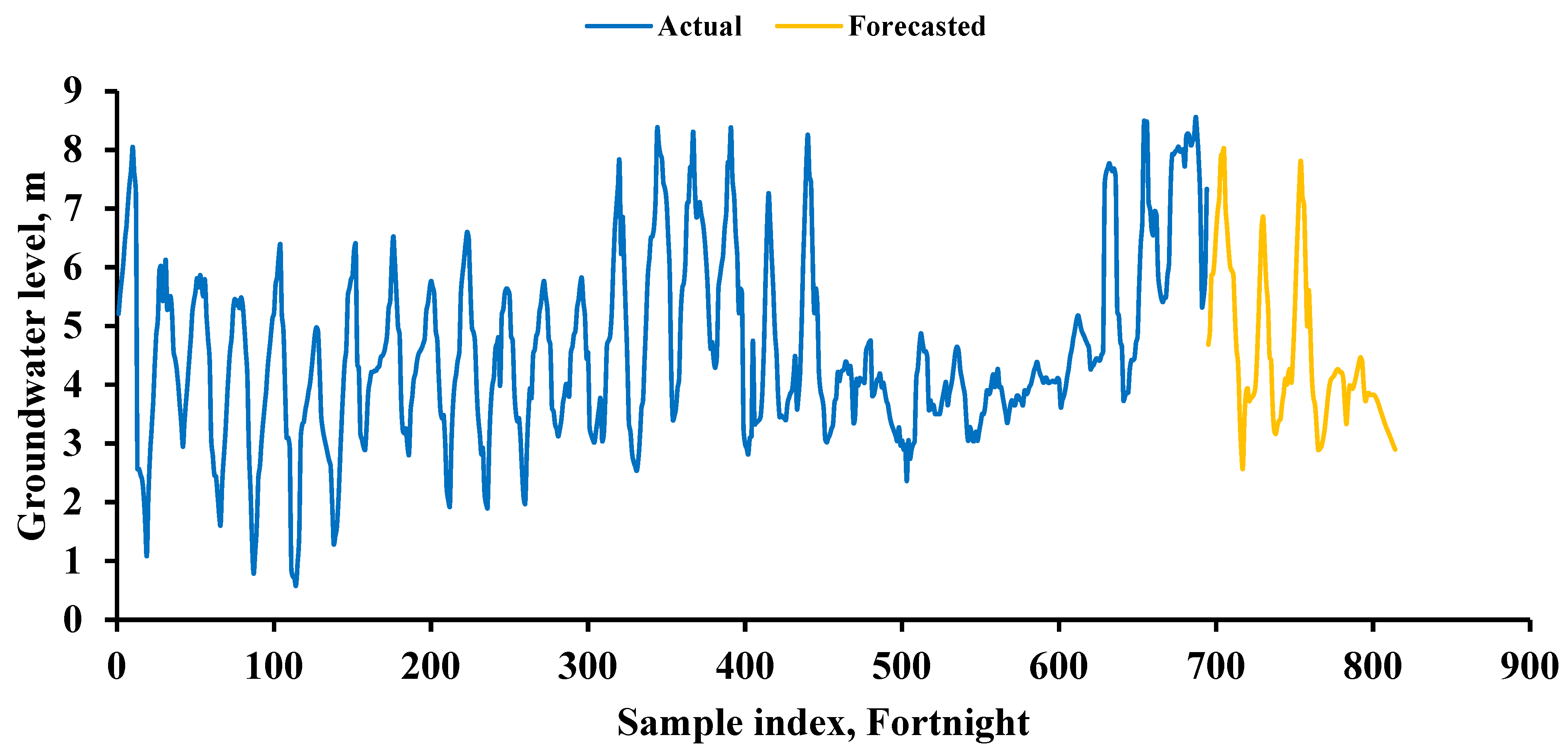
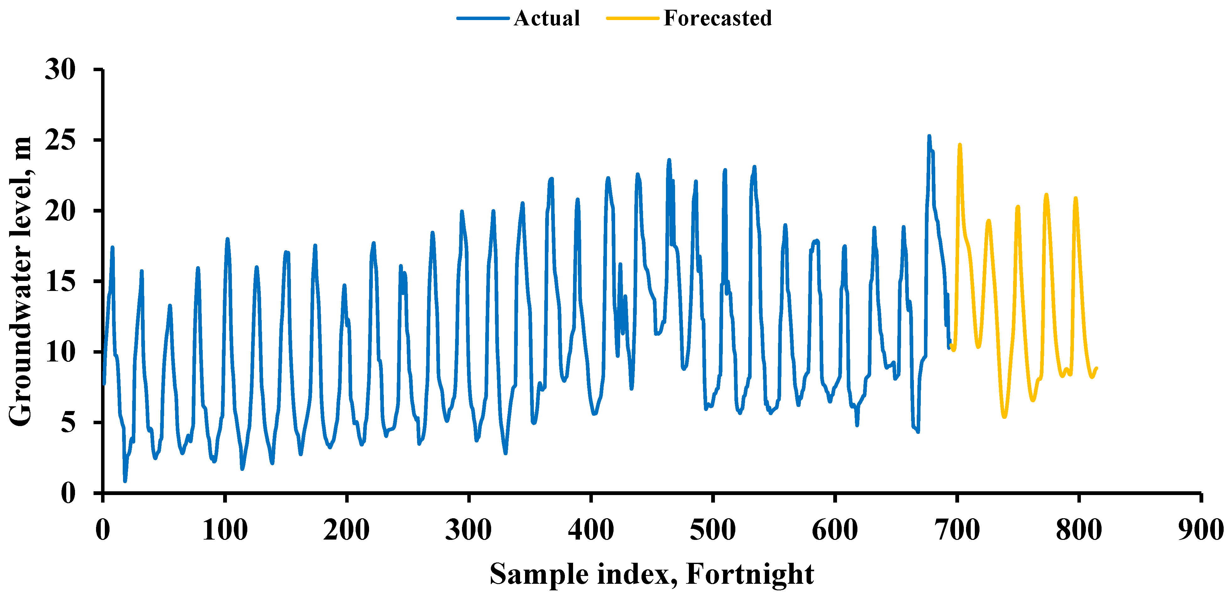
This study implemented standalone GRU and LSTM models, a hybrid GRU–LSTM architecture, as well as GA- and PSO-optimized variants of GRU and LSTM to forecast future values of a time-ordered GWL dataset using lagged observations as predictors. The forecasting problem was formulated as a regression task with a sequential prediction structure. A single lag of one time interval (15 days) was adopted to construct the input–output mapping. Accordingly, the target sequence was constructed by advancing the original time series by one step, whereas the input variables were formed from the same series with the final data point removed. In this setup, each model successfully learned how to estimate the subsequent time-step value based on the preceding observation. For out-of-sample multiple-step projection outside the observed record, a closed-loop (recursive) prediction strategy was adopted. In this approach, future values were generated by iteratively using previously predicted outputs as inputs, eliminating the need for actual observations during the forecasting horizon. Specifically, for predicting values from time $t$ to $t + k$ based on observations from time 1 to $t - 1$, the prediction at time $i -1$ was used as the input to estimate the value at time $i$. This recursive framework is particularly suitable for generating long-term forecasts when true future observations are unavailable. To implement this procedure, the network states were first reinitialized using a state-reset operation, after which initial predictions were produced using the early portion of the predictor sequence. Subsequently, the internal model state was adjusted using the complete input sequence to ensure temporal consistency. Subsequent forecasts were generated in an iterative loop using the prediction function, with the internal state updated after each step. Using this strategy, a 5-year (120-time-step) projection was generated through repeatedly reinjecting the most recent prediction into the model. This framework allows flexible extension of predictions to any desired forecasting horizon, as no additional external inputs are required once the model is initialized. Notably, the first forecasted value corresponds to the last observed time step used for initialization. To enhance numerical stability and convergence performance, both predictors and outputs were normalized to have zero mean and unit variance. During evaluation, the test dataset was transformed using the same scaling parameters learned from the training data to ensure consistency between training and inference phases.

The GRU architecture comprised a layer with 128 hidden units. The number of hidden units defines the model’s representational capacity; while a larger number of units can enhance the ability to capture complex nonlinear relationships, it may also increase the risk of overfitting if not properly regularized. All GRU models were trained using the “Adam” optimization algorithm with a starting learning rate of 1 × 10⁻³ and a maximum of 500 training epochs. Similarly, the LSTM architecture included a layer with 128 hidden units. The same considerations regarding hidden unit selection and model complexity apply to the LSTM configuration. The training settings were consistent with those used for the GRU models, employing the “Adam” optimizer with a learning rate of 1 × 10⁻³ and 500 epochs. The hybrid GRU–LSTM model consisted of an LSTM layer with 128 hidden units, followed by a GRU layer with 64 hidden units. The training settings remained consistent with those used for the standalone GRU models, utilizing the “Adam” optimizer with a learning rate of 1 × 10⁻³ and 500 epochs. The GA- and PSO-tuned GRU and LSTM models employed configurations similar to the standalone GRU and LSTM models; however, key hyperparameters including the number of hidden units, learning rate, and number of epochs were optimized using GA and PSO techniques to enhance predictive performance.

The comparative results of optimized model parameters are reported in

Table 5. Optimum hyperparameters of the GA- and PSO-tuned GRU and LSTM models at Bagha–Arani station.

Models	Used Parameters	Optimal Parameters
GA-GRU	Population size = 100 Maximum generations = 1000	Best hidden units = 175 Best learning rate = 0.00311 Best epochs = 493
GA-LSTM	Population size = 100 Maximum generations = 1000	Best hidden units = 177 Best learning rate = 0.00438 Best epochs = 493
PSO-GRU	Population size = 100 Maximum iterations = 1000 w = 0.7; c1 = 1.5; c2 = 1.5	Best hidden units: 166 Best learning rate: 0.01000 Best epochs: 600
PSO-LSTM	Population size = 100 Maximum iterations = 1000 w = 0.7; c1 = 1.5; c2 = 1.5	Best hidden units: 108 Best learning rate: 0.01000 Best epochs: 600

.

Table 5 summarizes the optimized hyperparameters obtained from the GA and PSO tuning processes for the GRU and LSTM models at the Bagha–Arani station. In all four optimized configurations, a population size of 100 was consistently used to ensure a sufficient search space for candidate solutions. For the GA-based models (GA-GRU and GA-LSTM), the optimization process was conducted over a maximum of 1000 generations, whereas for the PSO-based models (PSO-GRU and PSO-LSTM), a maximum of 1000 iterations was employed. In the case of PSO, the “inertia weight” (w) was set to 0.7, while the “cognitive” and “social” acceleration coefficients (c1 and c2) were both assigned a value of 1.5, maintaining an appropriate balance between “exploration” and “exploitation” in the search process. The GA-GRU configuration identified an optimal network structure consisting of 175 hidden units, a learning rate of 0.00311, and 493 training epochs. Similarly, the GA-LSTM model yielded a comparable architecture with 177 hidden units, a slightly higher optimal learning rate of 0.00438, and the same number of epochs (493). These results indicate that the GA-based optimization converged toward relatively similar network complexities for both GRU and LSTM architectures, with minor variation in learning rate reflecting model-specific training dynamics. For the PSO-optimized models, the PSO-GRU configuration selected 166 hidden units with a learning rate of 0.01000 and 600 epochs, while the PSO-LSTM model identified a smaller network comprising 108 hidden units, also paired with a learning rate of 0.01000 and 600 epochs. Compared with the GA-based models, PSO resulted in a higher learning rate and longer training duration, suggesting a different convergence behavior characterized by more aggressive parameter updates and extended optimization cycles. Notably, the PSO-LSTM model required fewer hidden units than its GRU counterpart, indicating a simpler optimal internal representation for capturing the temporal patterns in the dataset. Overall, Table 5 highlights that both GA and PSO were effective in tuning key hyperparameters, namely the number of hidden units, learning rate, and number of epochs, though they converged to distinct optimal configurations. This variation reflects differences in the search mechanisms of GA and PSO and their influence on model complexity and training dynamics.

During model training, all sequences within each mini-batch were standardized to a uniform length using left-padding. This strategy ensured consistent input dimensions across batches while minimizing the risk of the recurrent neural network learning from padded values at the terminal portion of sequences. Following training, the models were evaluated using independent test data.

2.5. Computation Time

Table 6. Computation time of the model development process at Bagha–Arani station.

Model	Computation Time, s
GRU	41
LSTM	24
GRU-LSTM	57
GA-GRU	925
GA-LSTM	524
PSO-GRU	809
PSO-LSTM	456

presents the computation time required for developing different DL and metaheuristic-optimized models at the Bagha–Arani station. The results show a clear contrast between the relatively low computational cost of standalone DL models and the substantially higher processing time associated with the hybrid metaheuristic-optimized configurations.

Among the standalone models, the LSTM model required the least computation time (24 s), followed by the GRU model (41 s), while the hybrid GRU–LSTM architecture exhibited a moderately higher runtime of 57 s. This increase reflects the additional computational complexity introduced by combining two recurrent architectures within a single framework. In contrast, the GA- and PSO-tuned models required significantly higher computation times due to the iterative nature of the optimization procedures. The GA-GRU model recorded the highest computational cost among GA-based configurations at 925 s, followed by GA-LSTM with 524 s. Similarly, PSO-based optimization also led to substantial increases in runtime, with PSO-GRU requiring 809 s and PSO-LSTM requiring 456 s. The higher computation time in these cases is attributed to repeated model training across multiple candidate solutions during the evolutionary and swarm-based search processes. Table 6 highlights that while standalone GRU, LSTM, and hybrid models are computationally efficient, the integration of GA and PSO optimization significantly increases processing time due to iterative hyperparameter tuning and repeated evaluations of model performance. Importantly, it is noted that the computation time followed a similar trend across other study stations, with only slight variations in the absolute numerical values, indicating consistent computational behavior across different datasets.

Despite the increased computational cost, the optimized models generally yielded improved predictive performance compared with their standalone counterparts, particularly in terms of error reduction and correlation enhancement at several observation wells. However, the magnitude of improvement was not always proportional to the increase in computational effort, indicating a clear trade-off between accuracy gain and computational efficiency. From a practical perspective, standalone LSTM and GRU models offer a favorable balance for real-time or operational forecasting applications where computational resources and response time are critical. In contrast, GA- and PSO-optimized models are more suitable for offline modelling and strategic planning purposes, where higher accuracy is prioritized over computational cost. Importantly, the computation time followed a consistent pattern across all observation wells, with only minor variations in absolute values, confirming the robustness and scalability of the computational behavior across different datasets.

2.6. Performance Evaluation Metrics

The following statistical performance evaluation indices were employed to evaluate the performances of the proposed models:

Mean Absolute Error (MAE):

$$MAE=\mathrm{m}\mathrm{e}\mathrm{a}\mathrm{n}\left[\left|{GWL}_{i,A}-{GWL}_{i,P}\right|\right]$$

(15)

Root Mean Squared Error (RMSE) [82]

$$RMSE=\sqrt{{\displaystyle \frac{1}{n}}{\displaystyle \sum _{i=1}^n}{\left({GWL}_{i,A}-{GWL}_{i,P}\right)}^2}$$

(16)

Normalized RMSE [83]

$$NRMSE={\displaystyle \frac{RMSE}{\overline{{GWL}_A}}}$$

(17)

Correlation Coefficient (R) [84]

$$R={\displaystyle \frac{{\displaystyle {\sum }_{i=1}^n}\left({GWL}_{i,A}-\overline{{GWL}_A}\right)\left({GWL}_{i,A}-\overline{{GWL}_P}\right)}{\sqrt{{\displaystyle {\sum }_{i=1}^n}{\left({GWL}_{i,A}-\overline{{GWL}_A}\right)}^2}\sqrt{{\displaystyle {\sum }_{i=1}^n}{\left({GWL}_{i,P}-\overline{{GWL}_P}\right)}^2}}}$$

(18)

a²⁰ index:

$$a^{20}-index={\displaystyle \frac{K^{20}}{n}}$$

(19)

Index of Agreement (IOA) [85]

$$IOA=1-{\displaystyle \frac{{\displaystyle {\sum }_{i=1}^n}{\left({GWL}_{i,A}-{GWL}_{i,P}\right)}^2}{{\displaystyle {\sum }_{i=1}^n}{\left(\left|{GWL}_{i,P}-\overline{{GWL}_A}\right|+\left|{GWL}_{i,A}-\overline{{GWL}_A}\right|\right)}^2}}$$

(20)

Median Absolute Deviation (MAD) [86]

$$\begin{array}{l}MAD\left({GWL}_A,{GWL}_P\right)\\ =median\left(\left|{GWL}_{A,i=1}-{GWL}_{P,i=1}\right|,\left|{GWL}_{A,i=2}-{GWL}_{P,i=2}\right|,\dots ,\left|{HGW}_{A,i=n}-{GWL}_{P,i=n}\right|\right) for i\\ =1,2,\dots ,n\end{array}$$

(21)

where ${GWL}_{i,A}$ = observed GWL, ${GWL}_{i,P}$ = predicted GWL, $\overline{{GWL}_A}$ = mean of the actual GWL values, $\overline{{GWL}_P}$ = average of the projected GWL, $SD$ exemplifies the standard deviation of the recorded data, $n$ = quantity of GWL data, $K^{20}$ = quantity of test samples that have a ${GWL}_{i,A}/{GWL}_{i,P}$ value ranging between 0.80 and 1.20.

2.7. Identification of the Best Models

Model selection across the observation wells was performed using a combined CRITIC and EDAS framework. The CRITIC method was applied to derive the weighting coefficients of the selected evaluation metrics whereas EDAS technique utilized these weighting coefficients to determine the ranking of the competing models. The CRITIC–EDAS framework was employed as a systematic multi-criteria decision-making (MCDM) approach to objectively integrate multiple complementary performance indicators into a unified evaluation structure. Although this ranking procedure does not directly influence or improve predictive accuracy, its main contribution lies in improving the interpretability, consistency, and decision-support value of the model assessment process. In this study, the CRITIC–EDAS framework was implemented as a post-evaluation tool rather than a predictive modelling technique, providing an organized mechanism for synthesizing diverse statistical metrics into a single, transparent ranking of competing models. Importantly, the value of this framework did not stem from modifying or enhancing model outputs, but from offering a rigorous and transparent way to aggregate multi-metric performance information into an interpretable decision index. This is particularly relevant in groundwater modelling applications, where inherent trade-offs among accuracy, bias, and correlation-based metrics are common. In such contexts, the framework supports the selection of the most appropriate operational model by providing a clear, defensible, and reproducible basis for decision-making in complex, multi-objective evaluation scenarios.

A brief overview of both methodologies is presented in the following paragraphs.

2.7.1. CRiteria Importance Through Intercriteria Correlation (CRITIC) Method

In MCDM problems, deciding on the relative significance of evaluation criteria plays a fundamental role in ensuring robust and reliable decisions. A range of weighting strategies has been proposed in the literature, which are generally classified into subjective, objective, and hybrid approaches. Among these, objective weighting methods derive criterion importance directly from the structure of the decision matrix, thereby avoiding reliance on expert judgment [87]. One of the most widely adopted objective weighting techniques is the CRITIC approach, originally introduced by [60]. This approach determines criterion weights by simultaneously considering two key aspects: the degree of contrast or variability pertaining to every criterion, typically represented by its statistical dispersion (standard deviation), and the level of conflict or correlation among criteria [88]. By integrating these two components, CRITIC generates weights that reflect both the discriminatory power and the informational redundancy of each criterion.

Due to its robustness and data-driven nature, the CRITIC method has been extensively applied in various decision-making contexts, including corporate performance evaluation [60], cross-country e-government assessment [89], water resources management [90], and supplier or contract manufacturer selection problems [91]. Before implementing the CRITIC approach, it is assumed that the decision framework consists of $m$ alternative prediction models evaluated against $n$ performance criteria. Under this formulation, the CRITIC procedure is executed through a series of systematic computational steps as described in prior studies [91,92].

Step 1: Construct the “decision matrix” $X$, which represents the performance of each prediction model in relation to all assessment criteria. In the matrix, prediction models are arranged as rows, while criteria (objectives) are organized as columns.

$$X={\left[x_{ij}\right]}_{m\times n}=\left[\begin{array}{c}\begin{array}{ccc}{x}_{11}& x_{12}& \dots \\ x_{21}& x_{22}& \dots \\ ⋮& ⋮& \ddots \end{array}\\ \begin{array}{ccc}{x}_{m1}& x_{m2}& \dots \end{array}\end{array}\begin{array}{c}\begin{array}{c}{x}_{1n}\\ x_{2n}\end{array}\\ ⋮\\ x_{mn}\end{array}\right],i=1,2,\dots ,m and j=1,2,\dots ,n$$

(22)

$x_{ij}$ represents the performance of the $i\mathrm{t}\mathrm{h}$ prediction model on $j\mathrm{t}\mathrm{h}$ criterion.

Step 2: Normalize the “decision matrix” according to the equations below:

For beneficial criteria:

$$X_{ij}^{\mathrm{*}}={\displaystyle \frac{x_{ij}-\mathrm{m}\mathrm{i}\mathrm{n}\left(x_{ij}\right)}{\max \left(x_{ij}\right)-\min \left(x_{ij}\right)}},i=1,2,\dots ,m and j=1,2,\dots ,n$$

(23)

For non-beneficial (cost) criteria:

$$X_{ij}^{\mathrm{*}}={\displaystyle \frac{\mathrm{m}\mathrm{a}\mathrm{x}(x_{ij)}-x_{ij}}{\max \left(x_{ij}\right)-\min \left(x_{ij}\right)}},i=1,2,\dots ,m and j=1,2,\dots ,n$$

(24)

$X_{ij}^{\mathrm{*}}$ represents the normalized performance value of the $i\mathrm{t}\mathrm{h}$ prediction model on $j\mathrm{t}\mathrm{h}$ criterion.

Step 3: Derive the criteria weight based on both the statistical dispersion (standard deviation) of each criterion and its relationship with the remaining criteria. The weight ($w_j$) of the $j\mathrm{t}\mathrm{h}$ criterion is computed as:

$$w_j={\displaystyle \frac{C_j}{{\displaystyle {\sum }_{j=1}^n}{C}_j}}$$

(25)

where

$$C_j={\sigma }_j{\displaystyle \sum _{\acute{\mathsf{ȷ}}=1}^n}\left(1-r_{j\acute{\mathsf{ȷ}}}\right)$$

(26)

where, $C_j$ represents amount of data associated with $j\mathrm{t}\mathrm{h}$ criterion, ${\sigma }_j$ denotes the statistical dispersion (standard deviation) of the $j\mathrm{t}\mathrm{h}$ criterion, $r_{j\acute{\mathsf{ȷ}}}$ represents the correlation coefficient between $j\mathrm{t}\mathrm{h}$ and $\acute{\mathsf{ȷ}}\mathrm{t}\mathrm{h}$ criteria. To evaluate the contrast among criteria, the statistical dispersion (standard deviation) of the standardized values within each column and the correlation coefficients between every pair of columns are considered [93]. A criterion is assigned a larger weight when it shows higher variability, as indicated by a greater standard deviation, and when it has weaker correlations with the remaining criteria [94]. In essence, a larger value of $C_j$ indicates that the criterion contributes more unique information to the decision formulation procedure, thereby justifying a higher weight for that criterion.

2.7.2. Evaluation Based on Distance from Average Solution (EDAS)

The EDAS approach was proposed by [95]. The central concept of this approach is the assessment of each alternative based on its deviation from the central (mean) solution as opposed to the ideal case or anti-ideal reference points [96]. In this framework, two key measures are defined: the Positive Distance from Average (PDA), which represents the extent to which an alternative performs better than the mean solution, and the Negative Distance from Average (NDA), which quantifies the degree to which an alternative shows inferior performance to the mean value [95]. The final ranking of alternatives is obtained by simultaneously considering these two measures to identify the most favorable option.

Owing to its simplicity and effectiveness, the EDAS method has been widely applied in various decision-making contexts. Applications include inventory classification as well as comparative evaluations against other established MCDM techniques such as COPRAS, TOPSIS, VIKOR, and SAW [95]. It has also been effectively employed in contractor selection problems [97] and in the selection of material handling equipment [98].

The procedural phases of the EDAS method are systematically outlined in the subsequent section, as described in prior studies [95].

Step 1: Given a set of $m$ candidate prediction models [$A_i\left(i=1,2,\dots ,m\right)$] and $n$ performance measures [$C_j\left(j=1,2,\dots ,n\right)$] in the context, construct the assessment table similar to one presented in Equation (22).

Step 2: The mean or average solution (AV) is computed by accounting for every criterion.

$$AV={\left[{AV}_j\right]}_{1\times n}$$

(27)

where

$${AV}_j={\displaystyle \frac{{\displaystyle {\sum }_{i=1}^m}{x}_{ij}}{m}}$$

(28)

Step 3: Compute the PDA and NDA matrices based on whether the criterion is classified as benefit or cost. PDA and NDA reflect how much every available option differs from the mean or average solution.

$$PDA={\left[{PDA}_{ij}\right]}_{m\times n}$$

(29)

$$NDA={\left[{NDA}_{ij}\right]}_{m\times n}$$

(30)

For beneficial $j\mathrm{t}\mathrm{h}$ criterion,

$${PDA}_{ij}={\displaystyle \frac{\mathrm{m}\mathrm{a}\mathrm{x}\left(0,\left(x_{ij}-{AV}_j\right)\right)}{{AV}_j}}$$

(31)

$${NDA}_{ij}={\displaystyle \frac{\mathrm{m}\mathrm{a}\mathrm{x}\left(0,\left({AV}_j-x_{ij}\right)\right)}{{AV}_j}}$$

(32)

For non-beneficial (cost) $j\mathrm{t}\mathrm{h}$ criterion,

$${PDA}_{ij}={\displaystyle \frac{\mathrm{m}\mathrm{a}\mathrm{x}\left(0,\left({AV}_j-x_{ij}\right)\right)}{{AV}_j}}$$

(33)

$${NDA}_{ij}={\displaystyle \frac{\mathrm{m}\mathrm{a}\mathrm{x}\left(0,\left(x_{ij}-{AV}_j\right)\right)}{{AV}_j}}$$

(34)

${PDA}_{ij}$ and ${NDA}_{ij}$ denotes the higher and lower deviation of the $i\mathrm{t}\mathrm{h}$ prediction models from the mean or average solution from the perspective of $j\mathrm{t}\mathrm{h}$ criterion. The best option is the one that demonstrates a higher PDA quantity and a smaller NDA quantity compared with the other available options [96].

Step 4: The PDA weighted total (${SP}_i$) and the NDA weighted total (${SN}_i$) for all prediction models are computed.

$${SP}_i={\displaystyle \sum _{j=1}^n}{w}_j{PDA}_{ij}$$

(35)

$${SN}_i={\displaystyle \sum _{j=1}^n}{w}_j{NDA}_{ij}$$

(36)

$w_j$ is the weight of the $j\mathrm{t}\mathrm{h}$ criterion. $w_j$ is obtained from the CRITIC method (Equation (13)).

Step 5: The SP and SN values are normalized by considering all prediction models.

$$N{SP}_i={\displaystyle \frac{{SP}_i}{{\mathrm{m}\mathrm{a}\mathrm{x}}_i\left({SP}_i\right)}}$$

(37)

$$N{SN}_i={\displaystyle \frac{{SN}_i}{{\mathrm{m}\mathrm{a}\mathrm{x}}_i\left({SN}_i\right)}}$$

(38)

$N{SP}_i$ and $N{SN}_i$ denote normalized $SP$ and $SN$ values of the $i\mathrm{t}\mathrm{h}$ prediction models, in that order.

Step 6: In this final step, the appraisal scores ($AS$) of all prediction models are computed.

$${AS}_i={\displaystyle \frac{1}{2}}\left(N{SP}_i+N{SN}_i\right) 0\le {AS}_i\le 1$$

(39)

${AS}_i$ is the “appraisal score” of the $i\mathrm{t}\mathrm{h}$ prediction models. Finally, the prediction models are ordered based on their appraisal scores in descending order.

3. Results and Discussion

This section provides a thorough assessment of the proposed DL models, focusing on their predictive performance using the independent test dataset. The precision and robustness of the GRU, LSTM, hybrid GRU–LSTM, and GA- and PSO-tuned GRU and LSTM models were assessed through multiple statistical metrics to ensure reliable comparison. To identify the most suitable model, a MCDM framework according to the CRITIC–EDAS approach was employed, integrating various performance indicators into a unified ranking system. In addition, the capability of the selected optimal model was examined for forecasting beyond the available training and testing data, demonstrating its potential for reliable long-term prediction in practical applications.

3.1. Model Performance on Test Dataset

Following the training phase of the proposed modelling frameworks, their predictive performance was validated using an independent test dataset to ensure unbiased evaluation. The effectiveness and reliability of the models were examined through a comprehensive set of statistical indicators. These performance measures included the R and IOA to assess the strength and consistency of predictions, the a²⁰ index to evaluate acceptable deviation levels, and error-based metrics such as NRMSE, MAE, and MAD. The evaluation results of the DL models at Bagha–Arani station are presented in this subsection, while the evaluation results of the DL models at the other eight stations are provided in the Supplementary Information.

Table 7. Performances of prediction models on unseen test dataset (Bagha–Arani).

Models	Performance Indices
	R	IOA	a20	NRMSE	MAE, m	MAD, m
ARIMA	0.366	0.495	0.357	0.348	1.869	1.213
GA-GRU	0.749	0.771	0.507	0.252	1.299	0.769
GA-LSTM	0.879	0.906	0.739	0.149	0.735	0.433
GRU	0.724	0.707	0.290	0.285	1.630	0.624
LSTM	0.820	0.872	0.652	0.176	0.894	0.479
LSTM-GRU	0.809	0.858	0.667	0.189	0.934	0.482
PSO-GRU	0.846	0.891	0.725	0.153	0.737	0.369
PSO-LSTM	0.721	0.810	0.710	0.211	0.987	0.466

presents the evaluation results of the developed DL models on the unseen test dataset for the Bagha–Arani observation well. The DL models were assessed using a combination of correlation-based, agreement-based, and error-based statistical indices.

Among all models, the GA–LSTM model exhibited the best overall performance, attaining the highest values of R (0.879) and IOA (0.906) among all models, along with the largest a²⁰ index (0.739). Additionally, it yielded the smallest error values, including NRMSE (0.149), MAE (0.735 m), and MAD (0.433 m), indicating its strong predictive capability and robustness. The PSO-GRU model also performed competitively, with relatively high R (0.846) and IOA (0.891) values, and low error metrics (NRMSE = 0.153, MAE = 0.737 m, MAD = 0.369 m), suggesting that optimization techniques significantly enhance GRU performance. The standalone DL models exhibited comparatively lower performance. The LSTM model showed moderate accuracy (R = 0.820, IOA = 0.872), outperforming the basic GRU model (R = 0.724, IOA = 0.707), which also recorded the highest prediction errors (NRMSE = 0.285, MAE = 1.630 m). The hybrid LSTM-GRU model achieved intermediate performance, indicating that combining architectures does not necessarily guarantee superior results without effective parameter optimization. The GA-GRU and PSO-LSTM models exhibited mixed performances. While GA-GRU improved over the basic GRU in terms of accuracy, it still lagged behind optimized LSTM-based models. Similarly, PSO-LSTM showed acceptable agreement (IOA = 0.810) and a relatively high a²⁰ index (0.710) but suffered from comparatively higher error values. The benchmark ARIMA model exhibited the poorest predictive performance among all models, with an R value of 0.366, an IOA of 0.495, an a²⁰ of 0.357, an NRMSE of 0.348, and error magnitudes of 1.869 m (MAE) and 1.213 m (MAD), consistently underperforming all DL models across the evaluated metrics.

The results clearly indicate that model optimization significantly contributes to enhancing prediction accuracy. The outstanding predictive performance of the GA-LSTM suggests that integrating GA-based hyperparameter tuning with LSTM significantly improves the model’s capacity to learn intricate chronological dependencies and nonlinear patterns within the data. The comparatively strong performance of PSO-GRU further supports the importance of optimization techniques, demonstrating that even simpler architectures like GRU can achieve high accuracy when properly tuned. In contrast, the relatively weaker performance of standalone GRU and LSTM models highlights their limitations when default or non-optimized parameters are used. Interestingly, the hybrid LSTM-GRU model did not outperform the optimized individual models, implying that architectural complexity alone does not guarantee better results. Instead, appropriate calibration and optimization of model parameters appear to be more influential factors. The findings suggest that the GA-LSTM model is the most reliable and accurate approach for predicting the target variable at the Bagha–Arani station. Its superior statistical performance across all evaluation metrics exhibits effective generalization ability and robust performance, indicating its suitability for real-world applications and future forecasting tasks.

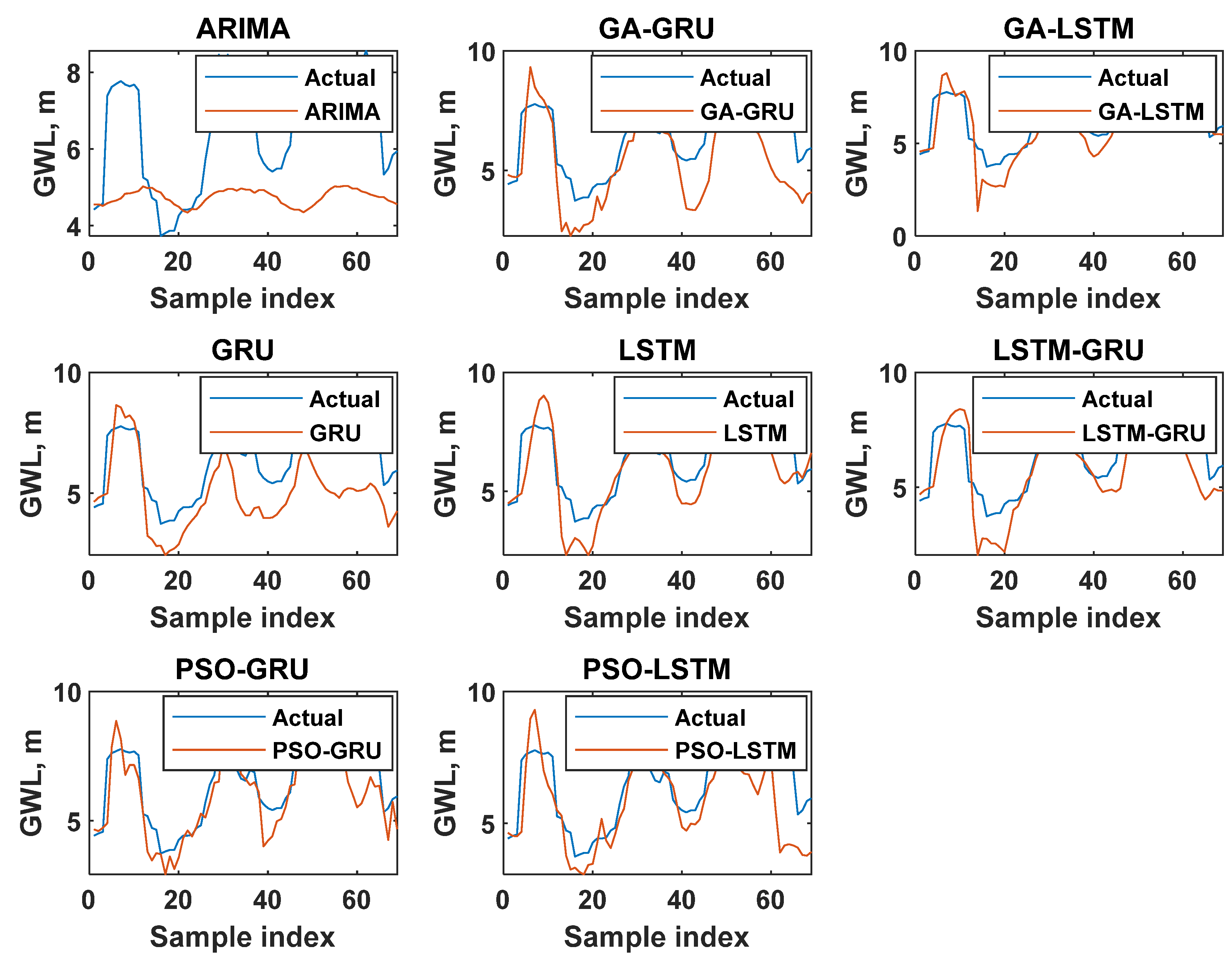
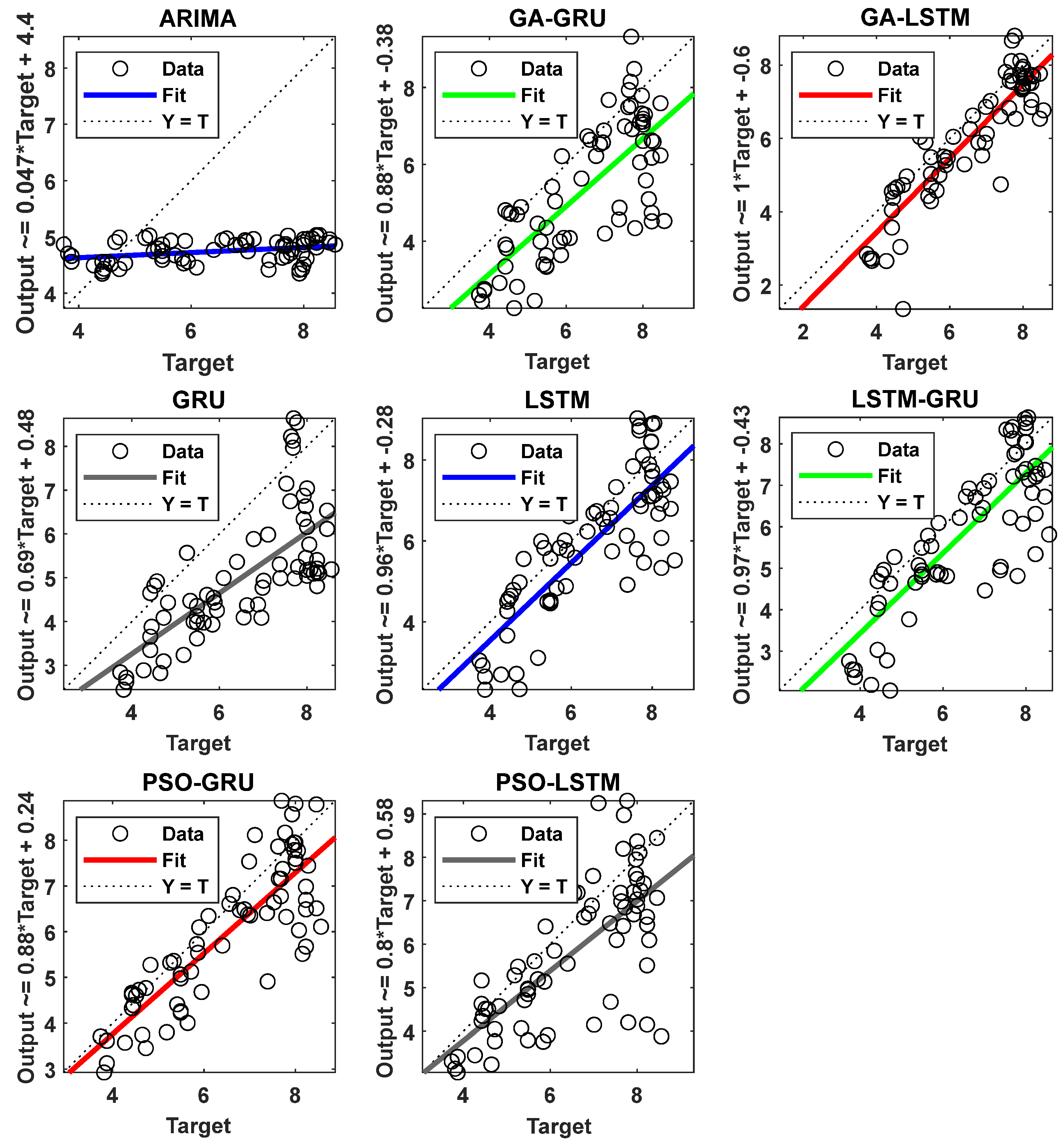
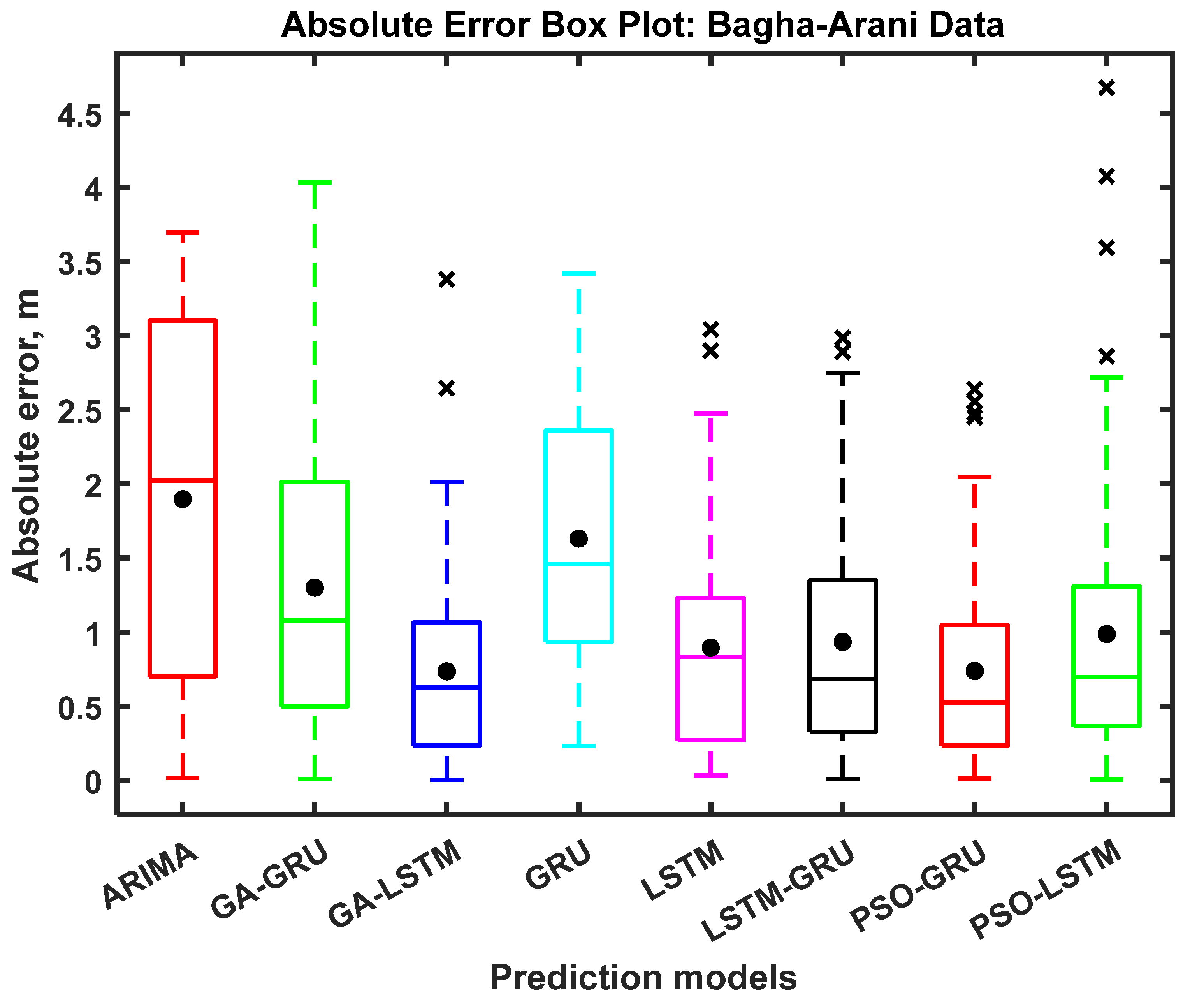
The model performance is further illustrated through a set of graphical analyses to provide deeper insight into prediction accuracy and error characteristics. Specifically, actual versus predicted time-series line graphs are used to visually compare the temporal alignment between observed and simulated values, highlighting the models’ ability to capture trends and fluctuations. In addition, regression plots are presented to examine the strength of the relationship between observed and predicted data, offering a clear indication of correlation and goodness-of-fit. Furthermore, absolute error box plots are included to depict the distribution, spread, and variability of prediction errors, allowing identification of median performance, dispersion, and potential outliers. These visual representations, shown in Figure 4, Figure 5 and Figure 6, complement the statistical evaluation and offer a thorough insight into the models’ predictive behavior.

Figure 4 presents a relationship between observed (actual) and model-predicted GWLs for the unseen test data at the Bagha–Arani monitoring well. The figure presents time-series line plots where the observed GWLs are plotted alongside the predictions generated by the DL models.

The plotted results show that the model predicted GWLs closely track the overall trend of the observed GWLs, indicating that the models are capable of capturing the underlying temporal patterns. Periods of rising and falling GWLs are reasonably well reproduced, suggesting that the models successfully learn the seasonal and short-term variations present in the dataset. However, slight deviations between observed and predicted values can be noticed at certain time steps, particularly during peak and low extremes, where some models tend to either underestimate or overestimate the GWLs. The strong agreement between the actual and model-predicted curves for the better-performing models (e.g., GA-LSTM and PSO-GRU, as indicated in the statistical analysis) demonstrates their strong ability to generalize on unseen data. These models exhibit minimal lag and reduced amplitude differences, indicating accurate tracking of both magnitude and timing of GWL changes. In contrast, comparatively weaker models (such as the standalone GRU) show more noticeable discrepancies, including larger deviations during extreme events and less consistent tracking of fluctuations. This suggests limitations in capturing complex nonlinear relationships and temporal dependencies when model parameters are not optimized. The figure also highlights that prediction accuracy is generally higher during stable periods, while larger errors tend to occur during abrupt changes or extreme conditions. This behavior is common in time-series modelling and indicates the inherent difficulty in predicting sudden variations in GWLs. Nevertheless, this graphical analysis confirms the findings from the statistical metrics, reinforcing that optimized and hybrid models provide more reliable and consistent predictions.

Figure 5 presents the regression plots illustrating the relationship between observed (actual) and model-predicted GWLs for the unseen test data at the Bagha–Arani observation well.

The regression plots clearly demonstrate variations in predictive accuracy among the different models. Models such as GA-LSTM and PSO-GRU show a strong linear relationship between observed and predicted values, as evidenced by the close grouping of points along the 1:1 line. This indicates high correlation, low bias, and strong generalization ability on unseen data. On the other hand, models like the standalone GRU display greater dispersion of points, reflecting weaker agreement and higher prediction errors. The spread of points away from the 1:1 line suggests the presence of both underestimation and overestimation across different GWLs. Another important observation is that prediction accuracy tends to decrease at extreme values, where the scatter becomes more pronounced. This indicates that while the models perform well for moderate GWLs, capturing extreme highs and lows remains more challenging. The regression analysis reinforces the statistical findings by visually confirming that optimized models outperform their non-optimized counterparts.

Figure 6 shows box plots of the absolute prediction errors for the evaluated models using the unseen test data at the Bagha–Arani observation well. The box plots provide a statistical summary of the distribution of absolute errors (i.e., absolute difference between actual and model-predicted GWLs) for each model. Key components of the box plot include the median (central line), interquartile range (IQR, represented by the box), whiskers indicating the spread of most data points, and potential outliers. This graphical representation enables a clear comparison of the central tendency, variability, and dispersion of prediction errors across all models. Models with smaller box sizes and lower median values indicate more accurate and consistent predictions, while larger boxes and longer whiskers reflect higher variability and less reliable performance.

The box plots presented in Figure 6 reveal notable differences in the error characteristics of the models. The GA-LSTM and PSO-GRU models exhibit relatively lower median absolute errors and narrower interquartile ranges, indicating high prediction accuracy and consistency. Their compact box structures suggest that most of the prediction errors are small and less variable, which aligns with their superior statistical performance. In contrast, models such as the standalone GRU show larger median errors and wider spreads, indicating less accurate and more inconsistent predictions. The presence of longer whiskers and potential outliers further suggests that these models occasionally produce large prediction errors, particularly under complex or extreme conditions. The LSTM and LSTM-GRU models demonstrate moderate performance, with reasonably low median errors but slightly wider distributions compared with the best-performing models. This indicates that while these models are generally reliable, their predictions exhibit greater variability. Another important observation is the presence of outliers in some models, which indicates occasional large deviations between observed and predicted values. These outliers are often associated with extreme GWL conditions, where prediction becomes more challenging. The box plot analysis confirms that optimized models (especially GA-LSTM and PSO-GRU) provide more stable and accurate predictions, with lower error dispersion and fewer extreme deviations. This graphical assessment complements the numerical performance metrics and highlights the robustness of the selected models for GWL prediction.

3.2. Selection of the Best Models

This section presents the adoption of a hybrid CRITIC–EDAS-based MCDM framework for the systematic evaluation and ranking of the developed predictive models. By integrating CRITIC and EDAS, this framework ensures that the model evaluation process is both objective in criterion weighting and robust in decision ranking, leading to a more reliable identification of the most suitable predictive model for each study location.

Table 8. Criteria weights of different performance evaluation indices calculated using CRITIC method.

Stations	Criteria Weight (CRITIC Method)
	R	IOA	a20	NRMSE	MAE	MAD
Bagha–Arani	0.176	0.167	0.170	0.174	0.169	0.144
Bagmara–Auchpara	0.153	0.187	0.185	0.200	0.142	0.133
Charghat–Charghat	0.174	0.166	0.179	0.157	0.160	0.164
Durgapur–Deluabari	0.190	0.171	0.169	0.154	0.141	0.175
Godagari–Godagari	0.190	0.229	0.169	0.127	0.127	0.157
Mohanpur–Raighati	0.187	0.168	0.163	0.163	0.164	0.154
Paba–Haripur	0.213	0.186	0.141	0.172	0.148	0.140
Puthia–Shilmaria	0.195	0.188	0.172	0.155	0.149	0.140
Tanore–Talondo	0.138	0.192	0.176	0.183	0.168	0.143

presents the objective weighting of different performance evaluation criteria derived using the CRITIC method for nine observation stations. The evaluated criteria include correlation-based and error-based indices, namely the R, IOA, a²⁰ index, NRMSE, MAE, and MAD. The CRITIC approach assigns weights in relation to both the variability of each criterion and the degree of conflict (correlation) among them, thereby ensuring an unbiased and data-driven importance ranking of evaluation metrics for each station.

The results show that the assigned weights vary slightly across stations, reflecting differences in model behavior and performance sensitivity at each location. In general, R and IOA consistently receive relatively higher weights, indicating their strong contribution to distinguishing model performance. For example, at the Paba–Haripur station, R attains the highest weight (0.213), while IOA also remains influential (0.186), suggesting that correlation and agreement measures are highly informative at this site. Similarly, at Godagari–Godagari, IOA achieves the highest weight (0.229), highlighting its dominant role in performance discrimination for that station. Error-based metrics such as NRMSE, MAE, and MAD also show notable contributions, particularly in stations where model errors vary significantly. For instance, NRMSE receives relatively higher importance at Bagmara–Auchpara (0.200) and Tanore–Talondo (0.183), indicating that normalized error plays a key role in differentiating model performance in these locations. Conversely, MAD generally receives comparatively lower weights across most stations, suggesting a relatively lower discriminatory power compared with other indices.

The CRITIC-based weighting results highlight that not all performance indices contribute equally to model evaluation, and their importance varies slightly across spatial locations. This confirms that model assessment is inherently site-dependent, influenced by variability and correlation structure of performance metrics at each station. Overall, R and IOA emerge as the most influential criteria, reflecting their strong ability to capture agreement and linear association between observed and predicted values. However, error-based indicators such as NRMSE and MAE also play a significant role in ensuring that magnitude-based prediction accuracy is adequately represented in the decision-making process. The relatively lower weights assigned to MAD across most stations suggest that it provides less unique information compared with other error metrics, possibly due to redundancy with MAE and NRMSE. Meanwhile, the variation in criterion weights across stations indicates that the contribution of each metric is not fixed but adapts to local data characteristics and model performance variability. In summary, the CRITIC method provides an objective and robust framework for determining the relative importance of evaluation criteria, ensuring a balanced integration of multiple performance indices in the subsequent EDAS-based model ranking process.

Table 9. Model weights and ranking calculated using EDAS method.

Models	Model Weights and Ranking
	Bagha-Arani		Bagmara-Auchpara		Charghat-Charghat		Durgapur-Deluabari		Godagari-Godagari		Mohanpur-Raighati		Paba-Haripur		Puthia-Shilmaria		Tanore-Talondo
	Weights	Rank	Weights	Rank	Weights	Rank	Weights	Rank	Weights	Rank	Weights	Rank	Weights	Rank	Weights	Rank	Weights	Rank
GA-GRU	0.179	6	0.837	3	0.000	7	0.237	5	0.724	3	0.694	2	0.000	7	0.000	7	0.556	3
GA-LSTM	0.997	2	0.000	7	1.000	1	0.264	6	0.579	5	1.000	1	0.553	4	0.234	6	0.718	2
GRU	0.000	7	0.112	5	0.450	4	1.000	1	1.000	1	0.637	3	0.915	3	0.958	2	1.000	1
LSTM	0.716	3	1.000	1	0.427	5	0.742	2	0.347	6	0.561	4	0.964	2	0.243	5	0.000	7
LSTM-GRU	0.663	4	0.887	2	0.490	3	0.062	7	0.729	2	0.557	5	0.413	5	1.000	1	0.506	4
PSO-GRU	1.000	1	0.737	5	0.419	6	0.304	4	0.022	7	0.000	7	0.344	6	0.594	3	0.130	6
PSO-LSTM	0.589	5	0.004	6	0.546	2	0.487	3	0.669	4	0.434	6	1.000	1	0.464	4	0.345	5

summarizes the ranking outcomes of the different predictive models across multiple observation well locations, as obtained using the CRITIC–EDAS multi-criteria decision-making framework. This table provides a comparative assessment of seven DL-based models evaluated over nine observation wells, integrating multiple performance indicators into a single ranking scheme. As the ARIMA consistently demonstrated inferior performance relative to all DL models across all observation wells and evaluation metrics, it was excluded from the model-ranking procedure. For each location, the models are assigned ranks ranging from 1 to 7, where a rank of 1 denotes the most effective and reliable model, while a rank of 7 corresponds to the lowest-performing alternative. This ranking structure facilitates a clear and systematic comparison of model performance across spatially distributed sites, enabling the identification of the most suitable modelling approach for each observation well.

It is observed from Table 9 that across the Bagha–Arani station, PSO-GRU achieved the highest weight (1.000), indicating superior performance, while GRU performed the weakest with a weight of 0.000. In contrast, for the Bagmara–Auchpara site, LSTM emerged as the best-performing model (weight = 1.000, rank = 1), followed closely by LSTM-GRU, while GA-LSTM performed poorly with a weight of 0.000. At the Charghat–Charghat location, GA-LSTM and PSO-LSTM demonstrated strong performance, with GA-LSTM achieving the top rank (weight = 1.000, rank = 1), whereas PSO-GRU showed relatively lower suitability. For the Durgapur–Deluabari well, GRU ranked first with a perfect weight (1.000), highlighting its strong predictive capability at this site, while LSTM-GRU performed the weakest. At Godagari–Godagari, GRU again dominated with the highest weight (1.000), whereas PSO-GRU showed the lowest performance. A similar pattern of variability is observed at Mohanpur–Raighati, where GA-LSTM achieved the highest score (1.000), indicating strong adaptability, while PSO-GRU performed poorly. At the Paba–Haripur site, PSO-LSTM ranked highest (weight = 1.000), suggesting that PSO-based optimization significantly improved LSTM performance at this location, whereas GA-GRU showed comparatively lower performance. In the case of Puthia–Shilmaria, LSTM-GRU emerged as the best-performing model (weight = 1.000), indicating strong hybrid model capability at this site, while GA-GRU performed the weakest. Finally, for the Tanore–Talondo station, GRU achieved the highest rank (weight = 1.000), whereas LSTM recorded the lowest performance.

The EDAS-based ranking results reveal a clear spatial variability in model performance across observation wells, indicating that no individual model continually outperforms others at all locations. Instead, the most suitable model varies depending on site-specific hydrogeological and data characteristics. Overall, GRU and LSTM-based models provided reliable performances across the stations, suggesting that recurrent neural networks are generally effective for capturing temporal dependencies in the dataset. However, their performance is not uniform across all sites, highlighting the sensitivity of model accuracy to local conditions. The results also demonstrate that hybrid and optimized models (e.g., GA-LSTM, PSO-GRU, LSTM-GRU) can achieve superior performance at specific locations, confirming the importance of parameter optimization and architectural enhancement. For instance, PSO-GRU and LSTM-GRU achieved top rankings in certain wells, indicating their ability to adapt better to complex nonlinear patterns in those cases. Interestingly, some optimized models such as GA-GRU and PSO-LSTM showed inconsistent performance, performing very well in certain locations but poorly in others. This suggests that optimization algorithms may enhance model performance in some datasets but may not guarantee universal improvement across heterogeneous spatial conditions. In summary, the findings emphasize that model performance is highly location-dependent, and therefore, a site-specific model selection strategy is essential. The variability in model ranking across stations underscores the necessity of site-specific model selection and evaluation, rather than relying on a single modelling approach for all locations. This is congruent with the findings reported by [99], who stated that the model is less impacted by the specific algorithm selected and more by the informational quality of the input variables.

The observed spatial variability in model performance across the nine observation wells can be attributed to differences in local hydrogeological conditions and groundwater dynamics. Wells exhibiting deeper GWLs and higher fluctuation amplitudes, typically influenced by intensive abstraction and variable recharge conditions, tend to present more nonlinear and non-stationary temporal patterns. In such cases, optimized and more complex architectures such as GA-LSTM and hybrid LSTM–GRU models demonstrate superior performance due to their enhanced ability to capture long-term dependencies and abrupt changes in GWL dynamics. Conversely, in wells with relatively stable groundwater regimes and lower variability, standalone models such as LSTM or GRU perform comparably well, as the underlying temporal structure is less complex and more autocorrelation-driven. These results suggest that model suitability is not uniform across the study area but is instead conditioned by site-specific hydrogeological behavior. Areas with stronger seasonal variability, irrigation-induced stress, and rapid drawdown–recovery cycles benefit more from optimized and hybrid DL structures, whereas relatively stable aquifer zones can be adequately represented by simpler architectures. This spatially differentiated performance highlights the importance of considering local groundwater depth and fluctuation characteristics when selecting forecasting models, rather than relying on a single globally optimal model for all observation wells.

3.3. Forecasting Performance of the Models Beyond the Available Data

The long-term predictive capability of the calibrated DL models was further assessed using time-series plots that compare observed GWLs with model-generated future projections. These graphical analyses provide a visual evaluation of each model’s ability not only to reproduce the historical dynamics of GWL fluctuations, but also to extend those patterns beyond the available observation period for long-range forecasting. By comparing observed and projected hydrographs, the figures illustrate how effectively the selected models captured temporal behavior, including declining or rising trends, seasonal oscillations, and broader variability in groundwater responses. Forecasts of Bagha–Arani, Bagmara–Auchpara, Charghat–Charghat, and Durgapur–Deluabari observation wells are presented in Figure 7, Figure 8, Figure 9 and Figure 10, respectively, while forecasts for the other five observation wells are provided in Figures S25–S29 of the Supplementary Information.

Figure 7 depicts the observed and forecasted GWL series at the Bagha–Arani observation well employing the PSO-GRU, found to be the top-performing model for this location. The projected hydrograph indicates that the PSO-GRU effectively preserved the dominant temporal structure embedded in the historical record and produced physically reasonable future groundwater trajectories. The close continuity between actual and projected values suggests that the PSO-GRU model effectively learned the nonlinear relationships governing groundwater dynamics at this site and was able to extrapolate those relationships over the forecasting horizon. The projected series further indicates the persistence of long-term groundwater behavior, while reflecting the model’s capability to maintain trend stability during recursive forecasting.

At Bagmara–Auchpara station (Figure 8), the LSTM model yielded the highest predictive performance and produced future projections that closely follow the historical groundwater evolution. The forecast results suggest that the model captured both the long-term movement and recurrent temporal fluctuations in GWL, thereby providing credible estimates of future groundwater conditions. The alignment between observed and projected hydrographs also demonstrates the capability of the LSTM model to represent intricate time-based dependencies and maintain predictive consistency over extended forecasting periods. Such performance is particularly important in regions where groundwater systems are influenced by interacting climatic and anthropogenic stresses.

Figure 9 presents the observed and projected GWL comparison for the Charghat–Charghat station using the GA-LSTM model, which outperformed all other candidate models at this site. The forecasted hydrograph indicates that the model successfully retained the underlying trend and variability structure of the observed data while extending predictions into the future. The incorporation of genetic algorithm optimization appears to have enhanced the model’s capacity to identify suitable parameter combinations, thereby improving its generalization ability for long-term prediction. As a result, the projected groundwater trajectories generated by the GA-LSTM model exhibit stability and realism, supporting its effectiveness for sustained forecasting applications.

Similarly, Figure 10 provides an illustration of the GRU model’s forecasting performance at the Durgapur–Deluabari station, where it was identified as the optimal model. The projected GWLs show strong continuity with the historical observations and indicate that the GRU architecture effectively captured site-specific groundwater dynamics. The results also highlight the ability of the GRU model to generate reliable multi-step forecasts while maintaining temporal coherence throughout the projection period. This robustness is particularly valuable for long-term groundwater planning, where forecasting uncertainty tends to increase as the prediction horizon extends.

Collectively, the forecasting plots reveal that the selected DL models were able to reproduce the major features of historical groundwater variability across different hydrogeological settings and generate plausible long-term projections for all observation wells. Although some short-term fluctuations and abrupt transitional noise were not fully captured, the models consistently tracked the broader system dynamics, including long-term trends and seasonal responses. This behavior is expected in recursive multi-step forecasting, where uncertainty accumulates over time, yet the models maintained sufficient stability to preserve physically meaningful groundwater trajectories.

The consistency of these projections across multiple stations demonstrates the robustness of the proposed modelling framework and confirms the suitability of DL-based approaches for extended groundwater forecasting under data-driven conditions. More importantly, the projected GWL trends provide valuable insight into potential future groundwater availability and associated risks under continued climatic variability and groundwater extraction pressures. These findings underscore the practical value of the developed models as decision-support tools for climate-resilient irrigation scheduling, sustainable groundwater abstraction planning, drought preparedness, and adaptive water resources management in the study region.

The five-year GWL projections presented in this study are intended primarily to demonstrate the potential applicability of the developed DL frameworks for indicative long-term groundwater trend assessment rather than to provide exact deterministic predictions of future GWLs. While the developed models showed promising predictive capability, it is acknowledged that recursive forecasting approaches may lead to error accumulation and increased uncertainty over extended prediction horizons. Therefore, it is important to adopt more rigorous validation strategies in future studies to improve the robustness and reliability of long-horizon groundwater forecasting. Therefore, the five-year recursive forecasts presented in this study are intended to provide an indicative assessment of possible groundwater level trends rather than precise deterministic long-term predictions. It is acknowledged that recursive forecasting approaches may introduce cumulative errors over extended prediction horizons, which can increase uncertainty in long-term outputs. In the absence of rolling-origin validation, horizon-wise error decomposition, or explicit uncertainty quantification, the projected results should be interpreted with caution. Accordingly, the findings are presented as a supportive tool for understanding general groundwater level tendencies rather than for direct operational groundwater planning and management decisions.

4. Implications for Groundwater Management

This study’s results carry significant implications for sustainable groundwater management, specifically in drought-prone regions of Bangladesh where underground water acts as a main supply of irrigation water and domestic use. The demonstrated capability of standalone and hybrid DL models to accurately forecast GWLs provides a valuable decision-support tool for water managers and policymakers. Reliable forecasts enable proactive planning of groundwater abstraction, irrigation scheduling, and drought mitigation strategies, mitigating the probability of excessive abstraction and longer-term aquifer depletion. Recent studies have highlighted that DL models can effectively capture complex hydro-climatic interactions and significantly improve predictive accuracy, thereby enhancing water resource planning and management under changing climatic conditions [100,101].

Furthermore, the integration of advanced forecasting models into groundwater management frameworks can support early warning systems for groundwater droughts and water scarcity, which are increasingly critical under climate variability and intensifying anthropogenic pressures. In Bangladesh, where groundwater resources are under severe stress due to agricultural demand and climate change, predictive modelling can facilitate adaptive management approaches by identifying future deficits and enabling timely interventions. For instance, spatial and temporal predictions of GWLs can assist in optimizing well operation, artificial recharge planning, and conjunctive use of surface and groundwater resources. Such data-driven approaches are essential for improving resilience and contributing to the sustainable management of water resources over the long term, as emphasized in recent ML-based groundwater and drought assessment studies [100,102].

In addition, the spatial heterogeneity in model performance among various locations observed in this research highlights the requirement for site-specific groundwater management policies instead of a one-size-fits-all strategy. The application of hybrid and optimized models allows for tailored forecasting solutions that account for local hydrogeological and climatic factors. This is especially critical in heterogeneous regions like Bangladesh, where groundwater dynamics vary significantly across spatial scales. Overall, the adoption of DL-based forecasting frameworks can enhance evidence-based policymaking, improve water allocation efficiency, and contribute to sustainable groundwater governance in drought-affected regions.

The regional significance of this study extends beyond northwestern Bangladesh, as many semi-arid and drought-prone regions worldwide face similar challenges of groundwater depletion, climate variability, and limited monitoring data. The proposed integrated framework combining DL models, optimization algorithms, and multi-criteria decision analysis offers a scalable and transferable methodology for groundwater forecasting in other data-scarce regions. In South Asian agricultural systems, where groundwater irrigation sustains food production and rural livelihoods, improved forecasting can support climate adaptation planning, sustainable agricultural water management, and regional water security initiatives. Moreover, the findings provide useful insights for policymakers and water management agencies seeking to integrate artificial intelligence-driven tools into national groundwater monitoring and decision-support systems. By enabling more accurate and location-specific groundwater predictions, the proposed framework can contribute to achieving long-term sustainability goals, particularly in regions increasingly vulnerable to droughts, groundwater stress, and climate change impacts.

5. Conclusions

This study evaluated the performance of standalone and hybrid DL models, including GRU, LSTM, LSTM–GRU, and their optimized variants (GA- and PSO-based), for GWL forecasting in a drought-affected region of Bangladesh. The results demonstrate that model performance varies across locations, highlighting the importance of site-specific analysis. Among the evaluated models, optimized approaches, particularly GA-LSTM and PSO-GRU, consistently exhibited superior predictive capability at several observation wells, achieving higher correlation and agreement indices along with lower error values. However, in some locations, standalone models such as LSTM and GRU also outperformed optimized and hybrid configurations, indicating that increased model complexity does not always guarantee improved performance. The baseline ARIMA model demonstrated moderate predictive capability but consistently underperformed compared with the proposed DL models across all locations. To provide a classical benchmark for comparison, the ARIMA model was included in this study. It should be noted that this comparison is limited to ARIMA as a representative traditional time-series forecasting method. Therefore, while the DL models demonstrated superior performance over ARIMA in this case, the results should not be interpreted as a general superiority over all conventional forecasting approaches, but rather as evidence within the context of the selected benchmark.

The application of the CRITIC–EDAS framework further enabled a robust and objective ranking of models by integrating multiple performance criteria, confirming that the best-performing model differs depending on local hydrogeological conditions. This work makes a major contribution through the integration of DL techniques with a MCDM framework for comprehensive model evaluation. The use of CRITIC for objective weighting of performance indices and EDAS for ranking provides a systematic and unbiased approach to model selection. Additionally, the study demonstrates the effectiveness of hybrid and optimization-based DL models in capturing complex temporal dynamics of groundwater systems. The inclusion of multiple observation wells enhances the generalizability of the findings and provides valuable insights into spatial variability in model performance. The principal contribution of this study lies not in the development of entirely new DL algorithms, but in the integration and systematic evaluation of standalone, hybrid, and metaheuristic-optimized DL frameworks using a CRITIC–EDAS-based multi-criteria decision-making approach for GWL forecasting in a drought-affected and data-limited region. The study further demonstrates the applicability of these approaches for long-term recursive GWL projection to support informed groundwater planning and monitoring.

From a practical and policy perspective, the findings underscore the potential of DL-based forecasting tools to support sustainable groundwater management in drought-prone regions. Accurate predictions of GWLs can facilitate informed decision-making related to irrigation planning, groundwater abstraction, and drought mitigation. The exhibited capability of the models to forecast beyond the available data further enhances their applicability in long-term water resource planning and climate adaptation strategies. Importantly, the study highlights the need for adopting site-specific modelling approaches to improve prediction reliability and optimize resource management.

6. Future Research Directions

The present study adopts a streamlined and data-efficient modelling framework by utilizing GWL time series as the primary input, which can be viewed as a practical strength rather than a constraint. This approach enhances the transferability and applicability of the models in data-scarce regions, where comprehensive hydro-climatic datasets are often unavailable. By relying on readily accessible groundwater observations, the developed models remain computationally efficient and easier to implement across multiple observation wells. At the same time, this design provides a flexible foundation that can be readily expanded to incorporate additional variables in future work, thereby offering opportunities to further improve predictive performance and process representation. Similarly, the use of optimized and hybrid DL models demonstrates strong predictive capability, although their relatively higher computational demand highlights the importance of balancing model complexity with operational feasibility in real-world applications.

Building on this foundation, future studies could prioritize multi-source data integration to better capture the complex drivers of groundwater variability. Incorporating climatic variables such as rainfall, temperature, and evapotranspiration, along with land use patterns and groundwater abstraction data, can significantly enhance model robustness and physical relevance. The use of satellite-based observations, such as those provided by the National Aeronautics and Space Administration and the European Space Agency, offers a promising avenue for improving spatial and temporal data coverage, particularly in regions with limited ground-based measurements. Recent studies have demonstrated that combining remote sensing products with ML models can substantially improve hydrological predictions and water resource assessments [103,104].

Another important direction is the exploration of next-generation DL architectures, including attention-based models and transformer networks, which have shown enhanced capability to model long-range dependencies in time-series data. These models can potentially overcome some of the limitations of recurrent architectures such as GRU and LSTM. In addition, the integration of physics-informed or hybrid modelling approaches, which combine data-driven techniques with physically based groundwater models, can improve interpretability and ensure consistency with underlying hydrogeological processes. Such approaches are increasingly recognized for their ability to enhance both prediction accuracy and scientific understanding [105,106].

Despite the promising predictive performance achieved in this study, a few limitations should be acknowledged. The developed models were trained primarily using historical GWL time-series data, and the inclusion of additional hydro-meteorological and anthropogenic factors, such as rainfall variability, evapotranspiration, land use change, pumping intensity, and river–aquifer interactions, could further improve forecasting reliability and interpretability. In addition, although the optimized and hybrid DL models generally enhanced prediction accuracy, they also required higher computational resources and longer training times due to iterative hyperparameter optimization processes. The recursive forecasting strategy adopted for future prediction may also accumulate uncertainties over longer forecasting horizons. Therefore, future studies should explore uncertainty quantification, ensemble modelling, explainable artificial intelligence techniques, and hybrid physics-informed DL frameworks to improve model robustness, transparency, and long-term forecasting capability. Expanding the modelling framework using larger datasets and transfer learning approaches across different hydrogeological settings could also enhance the generalizability of the proposed approach.

Furthermore, future studies should focus on developing more robust long-term groundwater forecasting frameworks by incorporating rolling-origin validation, horizon-wise performance assessment, ensemble forecasting, and uncertainty quantification techniques. The integration of probabilistic prediction intervals and explainable artificial intelligence approaches could further enhance the reliability, transparency, and interpretability of DL-based groundwater prediction models. Additionally, incorporating hydro-meteorological, climatic, and anthropogenic variables into forecasting frameworks may improve model generalizability and support more effective groundwater management under changing environmental conditions.

Finally, extending the proposed framework to larger spatial scales and diverse hydrogeological settings will be crucial for assessing its generalizability and practical utility. Applying the models at basin or national scales, along with incorporating uncertainty analysis and ensemble modelling techniques, can provide more reliable and actionable forecasts for water resource management. These advancements will contribute to the development of more comprehensive, scalable, and decision-oriented groundwater forecasting systems, supporting sustainable management in drought-affected regions.