Benchmarking AstroCLIP for Galaxy Property Estimation: Reproduction, Robustness, and Embedding Analysis

Abstract

Large imaging and spectroscopic surveys now produce heterogeneous data at a scale that challenges supervised approaches which depend on scarce labels and task-specific retraining. In this paper, we conduct a systematic evaluation and analysis of AstroCLIP, a cross-modal self-supervised model that aligns galaxy images and optical spectra within a shared embedding space. Our overarching aim is to extend the released benchmark with a more fine-grained assessment of robustness and embedding behaviour. Using the released DESI and DESI Legacy Imaging Survey evaluation suite, we first reproduce the main downstream galaxy-property regression results and then extend the evaluation in two novel ways: (i) by stratifying predictive performance across a neighbour-count proxy for local environment density, and (ii) by comparing the suite’s observational categories labelled Low-z (Bright) and High-z (Faint). We further inspect the embedding space using UMAP and unsupervised clustering, and quantify cluster–property agreement using the adjusted mutual information (AMI). Across tasks, spectral embeddings consistently outperform image embeddings; for example, zero-shot prediction reaches $R^2=0.87$ for $log\left(M_{*}\right)$ and $R^2=0.63$ for $log\left(\mathrm{sSFR}\right)$. Under our environment proxy, moderate-density bins often yield the strongest predictive performance, while very sparse or crowded bins tend to underperform. Image-based predictions benefit substantially from the Low-z (Bright) subset, whereas spectral embeddings are more stable across the observational split. At the same time, UMAP and clustering reveal only weak discrete separation by individual physical properties, so the results are most consistent with useful information being encoded in a largely continuous rather than sharply clustered form.

1. Introduction

The rapid expansion of astronomical data from large-scale sky surveys has transformed observational astronomy. Instruments such as the Dark Energy Spectroscopic Instrument (DESI) now catalogue millions of celestial objects, producing vast quantities of data such as photometric images and spectroscopic observations [1]. The DESI Legacy Imaging Surveys provide wide-area optical imaging, while DESI itself supplies large public collections of calibrated galaxy spectra and associated catalogues [2,3]. This abundance of data offers major opportunities for discovery but also creates pressure on analysis methods that require labels, substantial manual curation, or retraining for each downstream task.

Conventional supervised learning approaches in astronomy face clear limitations in this setting. A major constraint is the need for large volumes of high-quality labelled data, which remain scarce and expensive to obtain [1]. Spectroscopic follow-up observations, which are required in order to determine properties such as redshift, stellar mass, and metallicity, are resource-intensive. In addition, many supervised models are designed for a single downstream target and as such offer limited flexibility when the scientific question changes [1].

Self-supervised learning (SSL) offers a plausible alternative. SSL methods learn useful representations from unlabelled data by solving auxiliary training objectives that encourage the model to capture structure without explicit supervision. In astronomy, SSL has been used for tasks including galaxy morphology classification [4], gravitational lens detection [5], and spectral analysis [6,7]. These methods suggest that informative latent representations can be learned directly from raw data, reducing dependence on curated labels.

However, most astronomical SSL work has focused on a single modality. Prior to AstroCLIP, image- and spectrum-based pipelines were typically developed separately [1]. This is important because images and spectra contain complementary information; images capture morphology, structure, and local context, whereas spectra more directly encode line features and information on stellar populations. A model that aligns both modalities may therefore support downstream inference more flexibly than a model restricted to one input type. AstroCLIP addresses this problem by learning a shared representation space for galaxy images and spectra [1]. The model first pretrains each modality separately using self-supervised objectives, then aligns the resulting encoders through cross-modal contrastive learning. The aligned embedding space can then be probed for downstream tasks such as galaxy property estimation and cross-modal retrieval.

The overall shape of this paper’s conceptual core is as follows. First, we evaluate how well frozen AstroCLIP embeddings support the prediction of four galaxy properties, namely, $log\left(M_{*}\right)$, $log\left(Z_{\mathrm{MW}}\right)$, $t_{\mathrm{age}}$, and $log\left(\mathrm{sSFR}\right)$. We then examine how the performance changes across two practically relevant stratifications: the local environment as approximated through a neighbour-count proxy, and the observational split labelled Low-z (Bright) versus High-z (Faint). Our primary metric is $R^2$, adopted for consistency with the released evaluation suite and because it facilitates comparison across targets with different scales. Lastly, we evaluate the frozen embeddings using a linear zero-shot model and a lightweight nonlinear few-shot model.

Scope and Contributions

Our aim is to clarify the empirical value and the practical limits of AstroCLIP by separating (i) a baseline reproduction of the released evaluation suite from (ii) targeted extensions that additionally examine robustness and representation structure. Concretely, we make three contributions: first, we reproduce the released AstroCLIP evaluation for galaxy property estimation, including comparisons against the corresponding unaligned encoders; second, we extend the baseline by stratifying predictive performance across a simple proxy for local environment density and across the observational categories labelled Low-z (Bright) and High-z (Faint); third, we analyse the embedding space using dimensionality reduction and clustering, including quantification of the agreement with binned physical properties using the adjusted mutual information. Throughout, we focus on predictive robustness and embedding behaviour rather than on attributions of causality concerning galaxy evolution or physical explainability.

2. Related Work and Background Summary

2.1. Astronomical Surveys and Paired Modalities

Astronomical datasets are rapidly increasing in size and complexity. DESI is a large spectroscopic survey that has publicly released calibrated optical spectra and derived catalogues [2]. Complementing this, the DESI Legacy Imaging Surveys provide wide-area optical imaging and associated catalogues for use in target selection and cross-matching [3]. In the present context, the important point is not the detailed instrument design but the availability of naturally paired galaxy images and spectra, which makes cross-modal representation learning feasible.

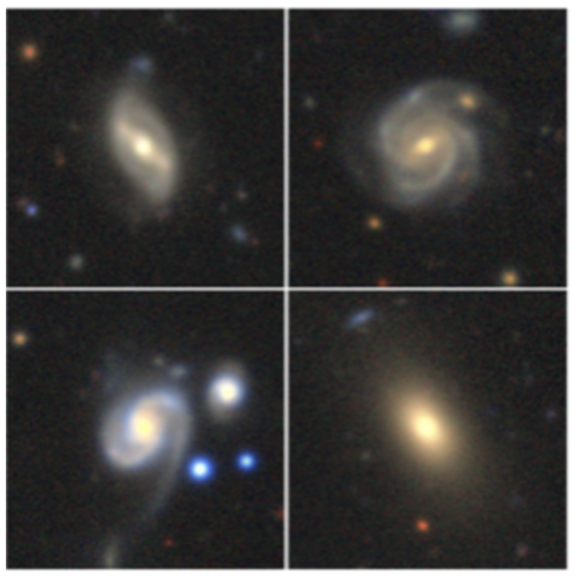
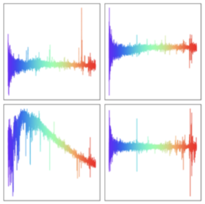
The modalities are illustrated in Figure 1 and Figure 2, which respectively show representative salient image detail and representative spectra.

2.2. Self-Supervised Learning in Astronomy

Self-supervised learning has already shown promise in several astronomical settings. Image-based work has used contrastive or self-distillation objectives to learn transferable representations for morphology and lensing [4,5,8]. Spectral work has used auto-encoding and unsupervised mapping to summarise large collections of spectra while preserving meaningful variation [6,7,9]. These lines of work suggest that compact latent representations can support downstream tasks even when explicit labels are scarce. However, while the released benchmark provides good empirical evidence of the model’s overall performance, it leaves a number of important questions unresolved, such as how sensitive that performance is to the observational setting and how the embedding space representation ought to be interpreted.

2.3. AstroCLIP in Relation to Prior Work

AstroCLIP combines separate self-supervised encoders for galaxy images and spectra with a contrastive alignment stage that brings both modalities into a shared latent space [1]. The aligned model can then be probed in zero-shot or few-shot settings for downstream property estimation. Note that in the present paper, “unaligned” does not refer to a different multimodal model; rather, it refers to the unimodal encoders prior to the cross-modal alignment step. Therefore, the comparison isolates the effect of cross-modal alignment, since both models start from the same unimodally pretrained encoders.

3. Methodology and Data

3.1. Data Sources

We use public galaxy data from DESI and the DESI Legacy Imaging Surveys (DESI-LS) [2,3]. Each galaxy in our evaluation set has both a DESI optical spectrum and a corresponding multi-band image cutout from DESI-LS, allowing for evaluation within each modality as well as through the cross-modal alignment learned by AstroCLIP [1]. The broader pretraining corpora described by Parker et al. [1] are large, with the DESI-LS image corpus containing tens of millions of non-stellar sources, whereas the paired image–spectrum subset used for alignment and downstream evaluation is far smaller. Therefore, the aim of the two-stage training scheme is to enable each encoder to first benefit from a much larger unimodal corpus before learning alignment on the paired subset.

3.2. Evaluation Targets and Protocol

For galaxy property estimation, we follow the evaluation protocol in the released suite. The downstream targets are $log\left(M_{*}\right)$, $log\left(Z_{\mathrm{MW}}\right)$, $t_{\mathrm{age}}$, and $log\left(\mathrm{sSFR}\right)$. “Zero-shot” results correspond to the supplied linear regressor applied to frozen embeddings. “Few-shot” results correspond to training a lightweight multilayer perceptron (MLP) on top of frozen embeddings using the suite’s 90/10 train/test split. Unless otherwise stated, all tables in Section 4 report test set performance. We use $R^2$ as the primary metric because it is the metric reported by the released AstroCLIP evaluation suite and because it allows comparison across target variables with different units and scales. For the stratified environment and brightness analyses, we evaluate both a k-nearest neighbours (KNN) regressor and an MLP regressor on frozen embeddings, as specified in the corresponding sections.

Considering that the aim of the present work is first to independently reproduce and verify the originally reported results and second to provide a further understanding of the method as released, by extending the depth of the analysis we purposefully do not introduce additional tuning beyond the released setup; hence, the few-shot MLP uses a single hidden layer of width 32, matching the configuration used in the evaluation suite.

For reproducibility,

Table 1. Model architecture and training infrastructure for each stage of the AstroCLIP pipeline.

Property	Image (DINOv2)	Spectra Transformer	AstroCLIP (CLIP)
Architecture	ViT-L (24 layers, 16 heads)	6-layer Transformer (6 heads)	Dual encoder + cross-attention
Parameters	∼307 M	∼43 M	—
Patch Size	$12\times 12$	20 (overlap 10)	—
Input Resolution	$144\times 144\times 3$	7514-d spectrum	Paired image–spectrum
Loss Function	DINO + iBOT + KoLeo	MSE (masked reconstruction)	InfoNCE
Hardware	16 × H100 GPUs	4 × H100 GPUs	1 × H100 GPU
Training Time	∼48 h	∼24 h	∼48 h

summarises the model architecture and training infrastructure for each stage of the AstroCLIP pipeline, while

Table 2. Training hyperparameters for each stage of the AstroCLIP pipeline [1].

Hyperparameter	Image (DINOv2)	Spectra Transformer	AstroCLIP (CLIP)
Training Length	200 epochs	500k steps	100 epochs
Batch Size	1536 (72/GPU × 16)	64	256
Embedding Dim.	1024	768	512
Optimiser	AdamW	AdamW ($\beta$: 0.9, 0.95)	AdamW
Learning Rate	2 × 10−4 (warmup + cosine)	1 × 10−5 (warmup + cosine)	1 × 10−4 (cosine)
Weight Decay	0.001 → 0.01	0.1	0.05
Gradient Clipping	3.0	1.0	1.0
EMA Momentum	0.992 → 1.0	—	—
Masking Strategy	iBOT ($\mathcal{U}(0.1, 0.5)$)	6 segments of length 30	None
Logit Scale	—	—	15.5 (fixed)
Drop Path Rate	0.3	—	—
Dropout	—	0.0	—

lists the corresponding training hyperparameters.

We also examine the released 90/10 train/test split at the level of the downstream target variables. At a coarse descriptive level, the train and test subsets show similar ranges and central tendencies across $log\left(M_{*}\right)$, $log\left(Z_{\mathrm{MW}}\right)$, $t_{\mathrm{age}}$, and $log\left(\mathrm{sSFR}\right)$, with no indication of a significant distributional mismatch that would cast doubt on the test set results. Hence, the test performance can be taken to reflect model behaviour under the released evaluation setting.

3.3. Embeddings and Baselines

We use the released frozen AstroCLIP encoders to compute fixed-length embeddings for images and spectra. Furthermore, we evaluate the corresponding unaligned encoders as a baseline. Here, “unaligned” means that the encoders have been pretrained within each modality but have not undergone the subsequent cross-modal alignment stage. This approach makes the baseline directly comparable to the aligned model and isolates the effect of cross-modal contrastive alignment rather than conflating it with the benefits of unimodal self-supervised pretraining.

3.4. Environment Proxy

To study robustness to local environment, we adopt the neighbour-count proxy implemented in Section 4.5. For each galaxy, we compute the nearest-neighbour angular separation, define a neighbourhood radius using an interquartile-range rule, count companions within this radius, and bin galaxies into ‘few’, ‘moderate’, and ‘many’ companions. Because this estimate is based on angular separations rather than full three-dimensional positions, it can be affected by projection effects, redshift-space distortions, and the selection properties of a flux-limited sample. Therefore, we interpret environment-linked differences as data illuminating robustness properties under this proxy, and do not claim that the differences provide evidence of causal environmental mechanisms.

3.5. Brightness Categories

The evaluation suite reports a two-way split labelled Low-z (Bright) and High-z (Faint). We adopt these subsets as given and interpret differences as sensitivity to observational setting, recognising that redshift, apparent brightness, and signal-to-noise are entangled in flux-limited samples; in other words, this split does not isolate a single factor, and any performance difference is likely driven by a combination of apparent brightness, redshift-dependent observational effects, and signal quality.

3.6. Embedding Space Analysis

To examine how physical properties are organised in embedding space, we apply dimensionality reduction (UMAP) for visual inspection and run clustering in the original embedding space. We quantify agreement between unsupervised clusters and binned physical properties using the adjusted mutual information (AMI). These analyses are intended to illuminate the understanding of the relevant representations rather than to provide evidence of physical organisation. We specifically highlight that weak separation in a two-dimensional projection does not imply the absence of relevant information in the full embedding; similarly, low AMI does not contradict good regression performance if the relevant information is encoded in a continuous rather than discretely clustered form.

3.7. Metrics

This section presents the metrics used for evaluation. Experiment-specific implementation details are described at the start of the relevant result subsections.

3.7.1. Coefficient of Determination ($R^2$)

The coefficient of determination, written as $R^2$, measures how much variation in a target variable Y is accounted for by predictions $\widehat{Y}$ relative to the sample mean baseline [10]. It is defined through the total and residual sums of squares, as follows:

$$S{S}_{\mathrm{tot}}=\sum _{i=1}^n{\left(Y_i-\overline{Y}\right)}^2,$$

(1)

where $\overline{Y}$ denotes the sample mean of the response variable Y. The residual sum of squares is

$$S{S}_{\mathrm{res}}=\sum _{i=1}^n{\left(Y_i-{\widehat{Y}}_i\right)}^2,$$

(2)

where ${\widehat{Y}}_i$ is the predicted value of $Y_i$ obtained from the regression model. The coefficient of determination is then

$$R^2=1-{\displaystyle \frac{S{S}_{\mathrm{res}}}{S{S}_{\mathrm{tot}}}}.$$

(3)

A higher $R^2$ indicates that predictions track the variation in the target more closely than the sample-mean baseline. In this paper, $R^2$ is used as an evaluation metric for both linear and nonlinear downstream regressions. As the benchmark metric used by the released AstroCLIP evaluation suite, this allows for the most consistent reproduction and comparison across targets.

3.7.2. Adjusted Mutual Information

The adjusted mutual information (AMI) is used to compare two partitions [11]. AMI adjusts mutual information for chance agreement, which makes it more suitable than raw mutual information when the number of clusters changes. In the present context, it measures the agreement between unsupervised cluster labels and bins derived from physical galaxy properties. It is defined as follows:

$$AMI(U,V)={\displaystyle \frac{MI(U,V)-\mathbb{E}\left[MI\right(U,V\left)\right]}{\mathrm{avg}\left(H\right(U),H(V\left)\right)-\mathbb{E}\left[MI\right(U,V\left)\right]}},$$

(4)

where $MI(U,V)$ denotes the mutual information between partitions U and V and where $H(·)$ denotes entropy. The AMI is symmetric and invariant to permutations of label identities [11]. In the present paper, low AMI should be interpreted as indicating weak agreement between discrete clusters and discretised target properties, not necessarily as the absence of predictive information in the embeddings.

4. Results

4.1. Galaxy Property Estimation (Baseline Reproduction)

In this subsection we reproduce the primary regression results reported for AstroCLIP [1], including comparisons against the corresponding unaligned encoders, setting the benchmark baseline for the rest of the paper. The later subsections extend this analysis by considering how performance changes across observational settings and by examining what insights the embedding space can reveal.

Here, our evaluation considers two experimental settings: zero-shot inference using the released linear probe, and few-shot learning using a single-hidden-layer MLP with width $w=32$. In both cases, evaluation is performed separately for image-derived and spectrum-derived embeddings. The baseline “Unaligned Transformer” refers to the respective image or spectrum encoder prior to cross-modality alignment. All values in

Table 3. Galaxy property estimation $R^2$ performance.

Source	Method	$\mathit{log}\left({\mathit{M}}_{*}\right)$	$\mathit{log}\left({\mathit{Z}}_{\mathit{MW}}\right)$	${\mathit{t}}_{\mathit{age}}$	$log\left(\mathbf{sSFR}\right)$
Images	AstroCLIP Zero-Shot	0.74	0.44	0.27	0.44
	AstroCLIP Few-Shot	0.73	0.43	0.26	0.42
	Unaligned Trans. Zero-Shot	0.65	0.40	0.16	0.25
	Unaligned Trans. Few-Shot	0.72	0.43	0.23	0.40
Spectra	AstroCLIP Zero-Shot	0.87	0.57	0.43	0.63
	AstroCLIP Few-Shot	0.88	0.58	0.43	0.64
	Unaligned Trans. Zero-Shot	0.84	0.57	0.38	0.62
	Unaligned Trans. Few-Shot	0.88	0.64	0.47	0.69

correspond to test set $R^2$.

For completeness, in 

Table 4. Galaxy property estimation $R^2$ performance on the training set.

Source	Method	$\mathit{log}\left({\mathit{M}}_{*}\right)$	$\mathit{log}\left({\mathit{Z}}_{\mathit{MW}}\right)$	${\mathit{t}}_{\mathit{age}}$	$log\left(\mathbf{sSFR}\right)$
Images	AstroCLIP Zero-Shot	0.77	0.47	0.27	0.48
	AstroCLIP Few-Shot	0.77	0.45	0.28	0.48
	Unaligned Trans. Zero-Shot	0.64	0.39	0.17	0.24
	Unaligned Trans. Few-Shot	0.73	0.42	0.21	0.39
Spectra	AstroCLIP Zero-Shot	0.88	0.57	0.41	0.63
	AstroCLIP Few-Shot	0.88	0.61	0.43	0.68
	Unaligned Trans. Zero-Shot	0.84	0.58	0.34	0.62
	Unaligned Trans. Few-Shot	0.89	0.65	0.47	0.70

we summarise the corresponding training set $R^2$ values for the same models and target properties. Taken together with Table 3, these values do not suggest a major train–test gap.

The results in Table 3 show that spectral embeddings produce the strongest overall predictive performance. In the zero-shot setting, the aligned spectral model attains $R^2=0.87$ for $log\left(M_{*}\right)$, $0.57$ for $log\left(Z_{\mathrm{MW}}\right)$, $0.43$ for $t_{age}$, and $0.63$ for $log\left(\mathrm{sSFR}\right)$, all of which exceed the corresponding image-based zero-shot scores. This is consistent with the intuition that spectra encode several of the target properties more directly than images.

In the few-shot setting, the gains are modest and uneven. For aligned spectra, the MLP regressor improves $log\left(M_{*}\right)$ and $log\left(\mathrm{sSFR}\right)$ slightly, while age remains unchanged. For aligned images, the changes are very small and can even be slightly negative, as for $log\left(M_{*}\right)$. For this reason, the few-shot improvements should be interpreted with due caution given that the observed benefits are small and uneven across targets even with bootstrap confidence intervals.

Compared with the unaligned encoders, cross-modal alignment is most clearly beneficial in the zero-shot image setting, with AstroCLIP improving $log\left(M_{*}\right)$ by 0.09 $R^2$ and $t_{\mathrm{age}}$ by 0.11 $R^2$ relative to the image-based baseline. On the spectral side the picture is more mixed, with zero-shot aligned embeddings slightly outperforming the zero-shot unaligned baseline on some properties but with the unaligned few-shot spectral model still exceeding the aligned one for $log\left(Z_{\mathrm{MW}}\right)$ and $log\left(\mathrm{sSFR}\right)$. The overall picture that emerges is that while cross-modal alignment does provide benefit, this benefit is not uniform across targets, modalities, and settings.

4.2. Confidence Intervals for Aligned vs. Unaligned Comparisons

To quantify the reliability of the performance differences reported above, bootstrap 95% confidence intervals (CIs) are computed for the $R^2$ scores of both aligned and unaligned models as well as for the difference $\Delta R^2$ between them.

Table 5. Bootstrap 95% confidence intervals for $R^2$ and $\Delta R^2$ (AstroCLIP minus unaligned baseline) using image embeddings.

Property	Model	Zero-Shot		Few-Shot
		${\mathit{R}}^{\mathbf{2}}$/$\Delta {\mathit{R}}^{\mathbf{2}}$	95% CI	${\mathit{R}}^{\mathbf{2}}$/$\Delta {\mathit{R}}^{\mathbf{2}}$	95% CI
$log\left(M_{*}\right)$	AstroCLIP	0.74	[0.732, 0.748]	0.73	[0.722, 0.738]
	Unaligned	0.65	[0.639, 0.661]	0.72	[0.710, 0.730]
	$\Delta R^2$	0.09	[0.083, 0.097]	0.01	[0.004, 0.017]
$log\left(Z_{\mathrm{MW}}\right)$	AstroCLIP	0.44	[0.425, 0.455]	0.43	[0.414, 0.446]
	Unaligned	0.40	[0.385, 0.415]	0.43	[0.414, 0.446]
	$\Delta R^2$	0.04	[0.032, 0.049]	0.00	[−0.008, 0.008]
$t_{\mathrm{age}}$	AstroCLIP	0.27	[0.256, 0.284]	0.26	[0.245, 0.275]
	Unaligned	0.16	[0.147, 0.173]	0.23	[0.214, 0.246]
	$\Delta R^2$	0.11	[0.100, 0.120]	0.03	[0.018, 0.042]
$log\left(\mathrm{sSFR}\right)$	AstroCLIP	0.44	[0.429, 0.451]	0.42	[0.407, 0.432]
	Unaligned	0.25	[0.239, 0.261]	0.40	[0.387, 0.413]
	$\Delta R^2$	0.19	[0.180, 0.200]	0.02	[0.010, 0.030]

and 

Table 6. Bootstrap 95% confidence intervals for $R^2$ and $\Delta R^2$ (AstroCLIP minus unaligned baseline) using spectral embeddings.

Property	Model	Zero-Shot		Few-Shot
		${\mathit{R}}^{\mathbf{2}}$/$\Delta {\mathit{R}}^{\mathbf{2}}$	95% CI	${\mathit{R}}^{\mathbf{2}}$/$\Delta {\mathit{R}}^{\mathbf{2}}$	95% CI
$log\left(M_{*}\right)$	AstroCLIP	0.87	[0.865, 0.875]	0.88	[0.876, 0.884]
	Unaligned	0.84	[0.835, 0.845]	0.88	[0.876, 0.884]
	$\Delta R^2$	0.03	[0.027, 0.033]	0.00	[−0.003, 0.003]
$log\left(Z_{\mathrm{MW}}\right)$	AstroCLIP	0.57	[0.556, 0.583]	0.58	[0.567, 0.593]
	Unaligned	0.57	[0.556, 0.583]	0.64	[0.628, 0.652]
	$\Delta R^2$	0.00	[−0.005, 0.005]	−0.06	[−0.066, −0.054]
$t_{\mathrm{age}}$	AstroCLIP	0.43	[0.413, 0.447]	0.43	[0.412, 0.448]
	Unaligned	0.38	[0.367, 0.393]	0.47	[0.452, 0.488]
	$\Delta R^2$	0.05	[0.042, 0.058]	−0.04	[−0.049, −0.032]
$log\left(\mathrm{sSFR}\right)$	AstroCLIP	0.63	[0.620, 0.640]	0.64	[0.631, 0.649]
	Unaligned	0.62	[0.610, 0.630]	0.69	[0.680, 0.700]
	$\Delta R^2$	0.01	[0.005, 0.015]	−0.05	[−0.057, −0.044]

report these intervals for zero-shot and few-shot evaluation on frozen embeddings.

For image embeddings, all $\Delta R^2$ confidence intervals under zero-shot evaluation exclude zero. The largest improvement appears for $log\left(\mathrm{sSFR}\right)$ ($\Delta R^2=0.19$, 95% CI $[0.180, 0.200]$), while the smallest, though still clearly positive, is for $log\left(Z_{\mathrm{MW}}\right)$ ($\Delta R^2=0.04$, 95% CI $[0.032, 0.049]$). Under few-shot evaluation, the interval for $log\left(Z_{\mathrm{MW}}\right)$ is around zero ($\Delta R^2=0.00$, 95% CI $[-0.008, 0.008]$), but the remaining three properties retain positive gaps.

For spectral embeddings, the results are different. Under zero-shot evaluation, AstroCLIP retains a significant advantage for $log\left(M_{*}\right)$ ($\Delta R^2=0.03$, 95% CI $[0.027, 0.033]$), $t_{\mathrm{age}}$ ($\Delta R^2=0.05$, 95% CI $[0.042, 0.058]$), and $log\left(\mathrm{sSFR}\right)$ ($\Delta R^2=0.01$, 95% CI $[0.005, 0.015]$), while the interval for $log\left(Z_{\mathrm{MW}}\right)$ is around zero ($\Delta R^2=0.00$, 95% CI $[-0.005, 0.005]$), indicating no benefit for metallicity in this setting. Under few-shot evaluation, the unaligned SpecFormer baseline slightly but consistently outperforms AstroCLIP, with all four $\Delta R^2$ intervals falling below zero. This is in line with the few-shot result in Table 3.

4.3. Embedding Space Analysis

In this section we examine what insights can be garnered from the embedding space as well as the limits of those insights. We do not hypothesise that physically meaningful information necessarily clusters neatly; instead, we are interested in the question of whether qualitative projections and simple clustering procedures are consistent with the downstream regression behaviour observed previously.

4.3.1. Dimensionality Reduction of Embeddings

Experimental Setup

UMAP was applied to reduce the high-dimensional embeddings to two dimensions for visualisation. The procedure followed the approach described by Hayat et al. [8]. Two sets of UMAP projections were generated: one using embeddings from the contrastive training with alignment, and another using embeddings from an unaligned baseline model.

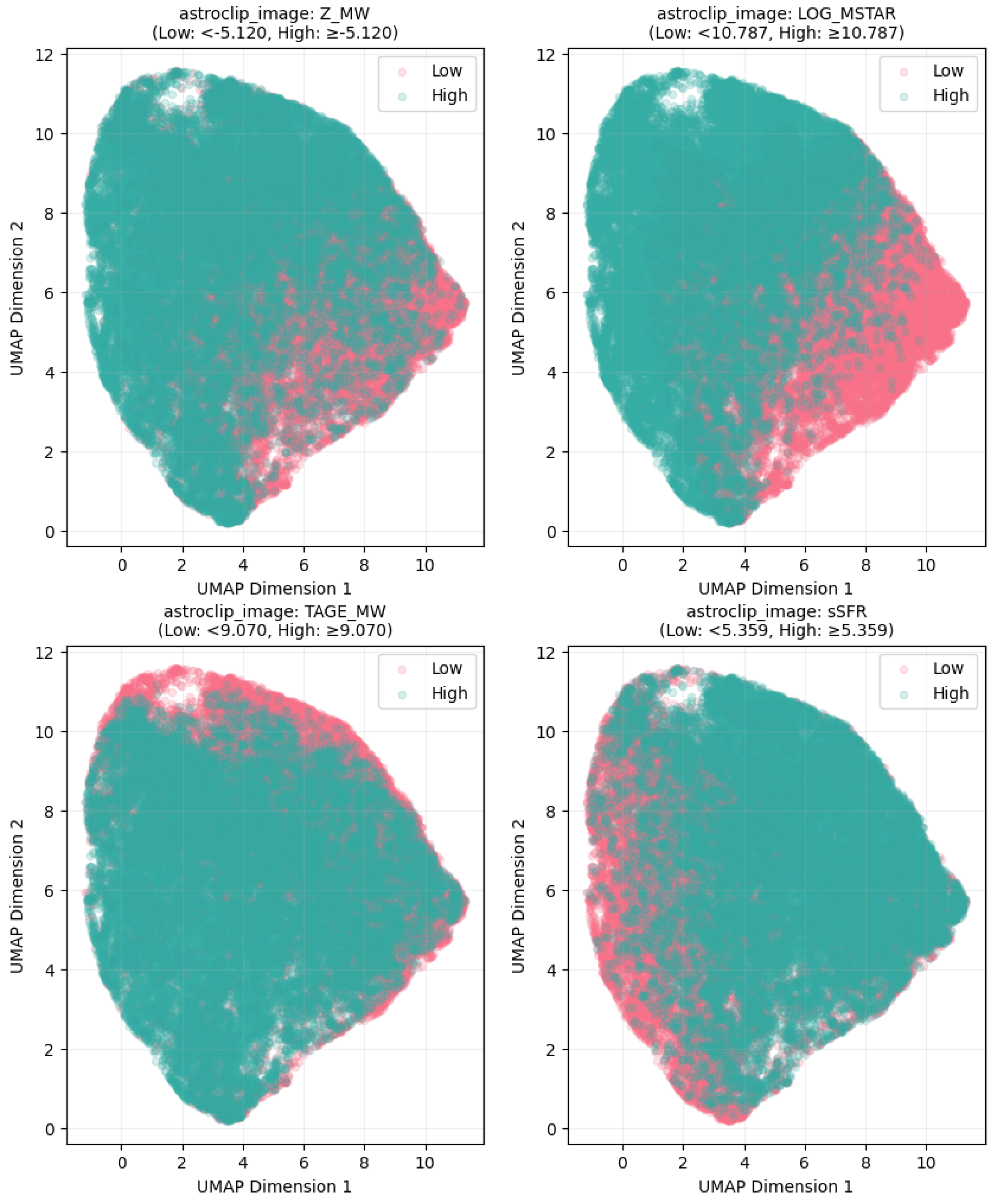
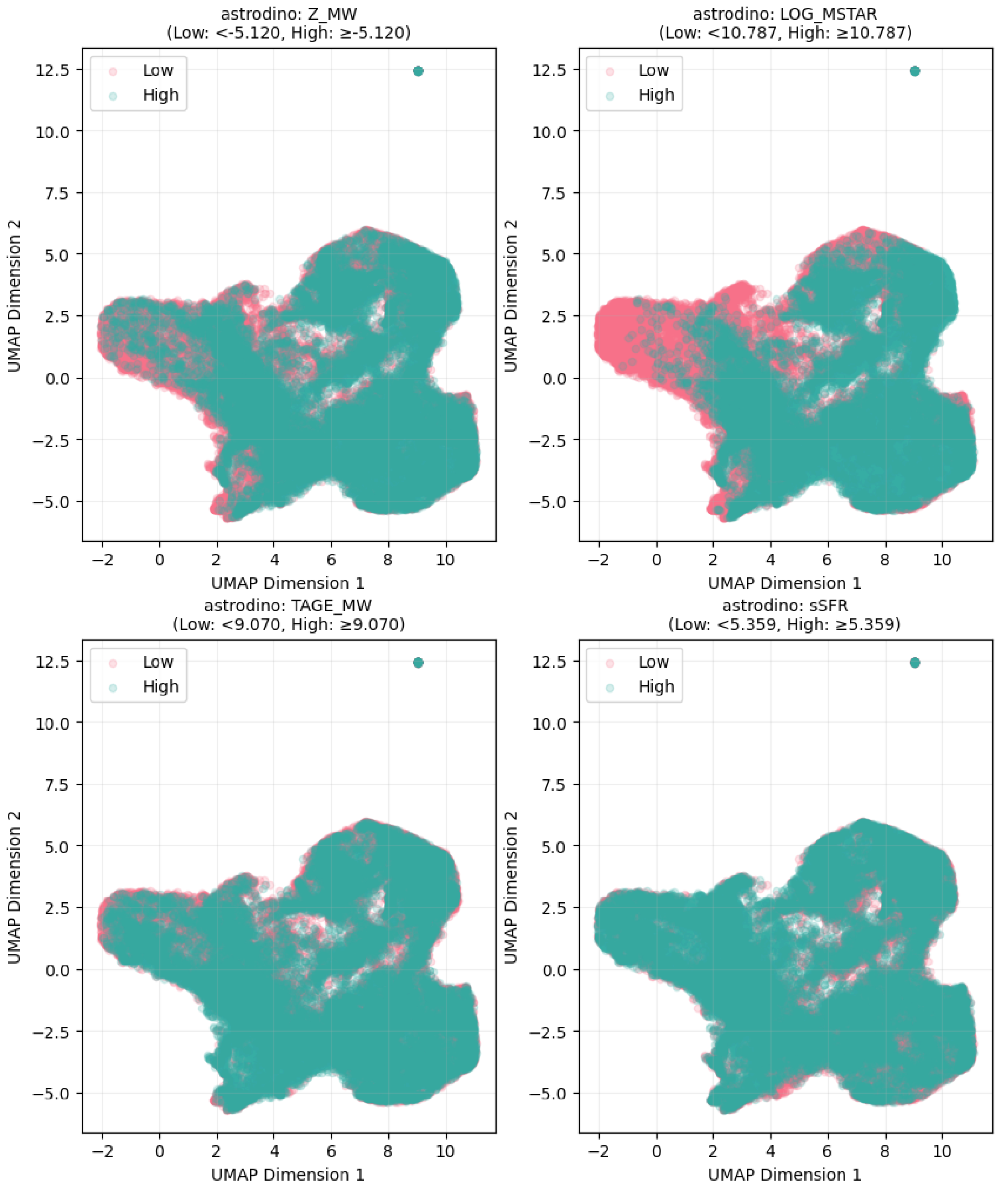
Embeddings were generated for both image-based and spectrum-based modalities. For each modality, galaxies were colour-coded according to binned physical properties. Continuous properties such as $log\left(M_{*}\right)$ and $log\left(\mathrm{sSFR}\right)$ were divided into low and high categories using quantile-based thresholds to ensure balanced class representation. We use these plots only as qualitative aids, and stress that apparent proximity or separation in two dimensions should not be treated as definitive evidence about the full embedding geometry.

Visualisation of Embeddings

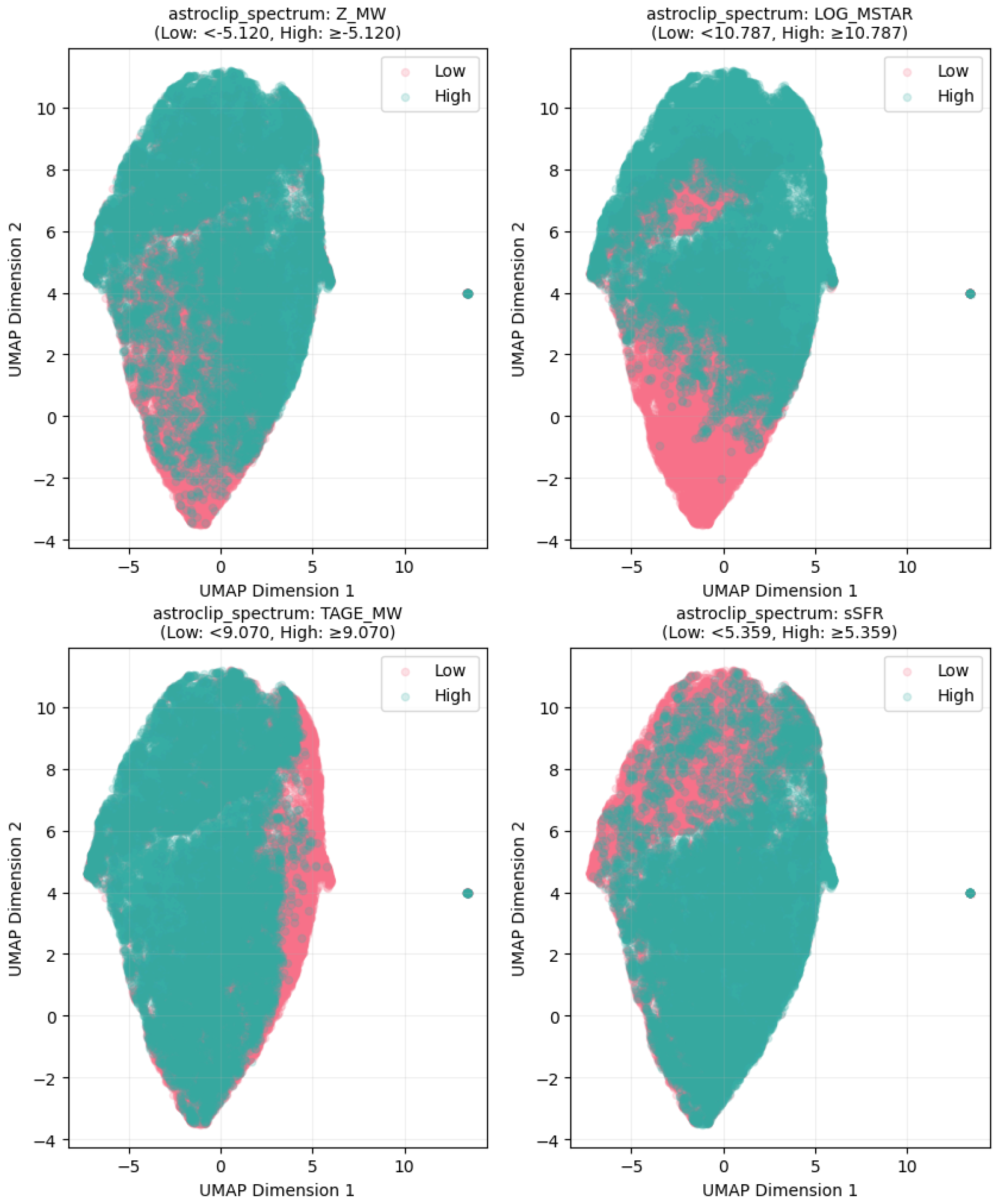
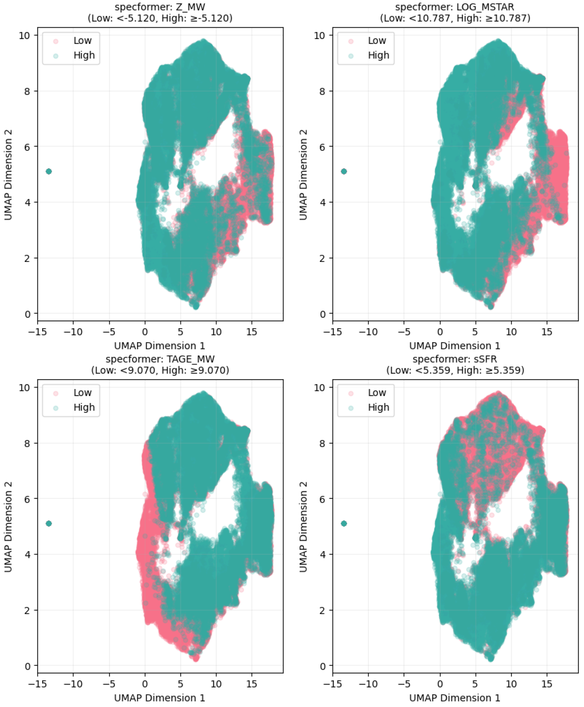
Figure 3 and Figure 4 show the aligned and unaligned image embeddings, respectively, while Figure 5 and Figure 6 show the corresponding spectral embeddings. For the image embeddings, the UMAP projections do not display sharply separated clusters in either the aligned or the unaligned plots. A partial concentration of high-mass points appears in restricted regions, especially for stellar mass; however, the overall separation between physical property bins remains weak. The projections suggest some degree of organisation, particularly for stellar mass, but do not support a claim that the learned image embeddings form neat property-specific clusters.

A similar pattern is observed for the spectrum embeddings. Again, stellar mass shows the strongest visual tendency towards local organisation, but the plots do not reveal neat discrete partitions. Taken together, our results show the embeddings can produce strong regression without yielding strong low-dimensional cluster separation. Therefore, the clustering analyses we present next are pursued as an examination of whether any discrete grouping is present at all, rather than as a necessary condition for downstream usefulness.

4.3.2. Clustering Analysis of Image Embeddings

Experimental Setup

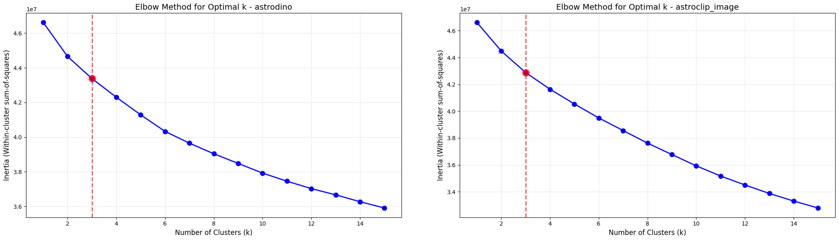
To assess whether image embeddings exhibit any useful discrete clustering, K-means clustering was applied to standardised embedding vectors for both the unaligned transformer (AstroDino) and AstroCLIP. The number of clusters k was varied from 1 to 15 and inertia was computed at each step. The corresponding inertia curves for the image embeddings are shown in Figure 7. The inertia curves do not show a sharp elbow, so the value $k=3$ was selected as a pragmatic choice adopted to enable direct comparison across models.

Quantitative Results

Table 7. Mean physical properties and cluster frequencies for AstroDino and AstroCLIP image embedding clusters ($k=3$).

Cluster	${\mathit{t}}_{\mathit{age}}$	$log\left({\mathit{Z}}_{\mathbf{MW}}\right)$	$log\left({\mathit{M}}_{*}\right)$	$log\left(\mathbf{sSFR}\right)$	Count
AstroDino 0	8.82	−4.96	11.00	4.04	15,100
AstroDino 1	8.63	−5.15	10.82	4.47	19,279
AstroDino 2	8.28	−5.97	10.12	5.67	11,148
AstroCLIP 0	8.47	−5.77	10.31	4.97	9408
AstroCLIP 1	8.77	−5.20	10.81	4.31	21,307
AstroCLIP 2	8.45	−5.11	10.82	4.86	14,812

summarises the mean values of selected physical galaxy properties in each of the three clusters identified for both models. The clusters show some variation in mean properties, especially in $log\left(M_{*}\right)$, but the separation is limited.

To quantify the relation between cluster assignments and physical properties, AMI scores were computed after binning each property into low, medium, and high categories.

Table 8. AMI scores between cluster labels and binned physical properties.

Model	Property	AMI Score
AstroCLIP	$t_{age}$	0.012
	$Z_{MW}$	0.014
	$log\left(M_{*}\right)$	0.038
	$log\left(\mathrm{sSFR}\right)$	0.003
AstroDino	$t_{age}$	0.007
	$Z_{MW}$	0.017
	$log\left(M_{*}\right)$	0.093
	$log\left(\mathrm{sSFR}\right)$	0.021

shows that all values are low, indicating weak agreement between discrete cluster assignments and individual physical properties. This finding suggests that whatever information the embeddings contain is not well captured by a simple partition into three clusters.

4.3.3. Clustering Analysis of Spectral Embeddings

Experimental Setup

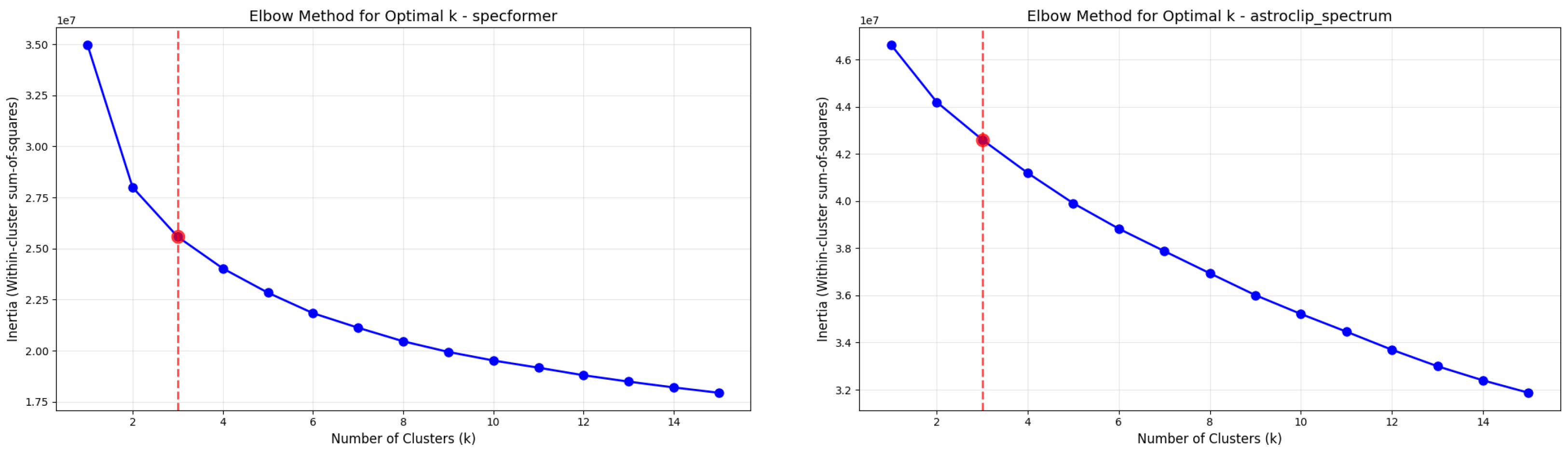
The same clustering procedure was repeated for spectral embeddings derived from the unaligned spectrum transformer (SpecFormer) and the aligned AstroCLIP model. Standardisation and the same exploratory choice of $k=3$ were used, as illustrated in Figure 8.

Quantitative Results

Table 9. Mean physical properties and cluster frequencies for SpecFormer and AstroCLIP spectral embedding clusters ($k=3$).

Cluster	${\mathit{t}}_{\mathit{age}}$	$log\left({\mathit{Z}}_{\mathbf{MW}}\right)$	$log\left({\mathit{M}}_{*}\right)$	$log\left(\mathbf{sSFR}\right)$	Frequency
SpecFormer 0	8.94	−4.95	10.96	2.88	14,400
SpecFormer 1	8.45	−5.20	10.81	5.33	21,978
SpecFormer 2	8.44	−6.05	10.07	5.66	9149
AstroCLIP 0	8.97	−5.42	10.67	4.77	10,538
AstroCLIP 1	8.45	−5.16	10.76	4.74	19,015
AstroCLIP 2	8.55	−5.36	10.68	4.38	15,974

reports the mean physical properties within each cluster. The differences between clusters are generally modest. An exception appears in the SpecFormer model, where $log\left(\mathrm{sSFR}\right)$ for Cluster 0 is notably lower than for Clusters 1 and 2.

AMI scores for the spectral models are provided in

Table 10. Adjusted mutual information scores between cluster labels and binned physical properties for spectral embeddings.

Model	Property	AMI Score
AstroCLIP	$t_{age}$	0.013
	$log\left(Z_{\mathrm{MW}}\right)$	0.009
	$log\left(M_{*}\right)$	0.006
	$log\left(\mathrm{sSFR}\right)$	0.002
SpecFormer	$t_{age}$	0.024
	$log\left(Z_{\mathrm{MW}}\right)$	0.079
	$log\left(M_{*}\right)$	0.093
	$log\left(\mathrm{sSFR}\right)$	0.062

. As with the image embeddings, all of the values are low, indicating weak agreement between discrete cluster labels and individual properties. SpecFormer shows somewhat stronger AMI than AstroCLIP for several targets. This suggests that alignment does not make the embedding space more discretely clusterable by these individual properties, even though the aligned embeddings remain strongly predictive features for regression. Again, this is compatible with a continuous encoding of relevant information.

4.3.4. HDBSCAN Clustering of Image Embeddings

Experimental Setup

This subsection examines whether a density-based clustering method can identify meaningful structures within the image embedding space. The clustering was performed using the HDBSCAN algorithm. The Euclidean distance metric was used for all clustering experiments. The min_cluster_size and min_samples parameters were varied during preliminary tests. A min_samples value of 5 was selected to encourage less conservative clustering, increasing the probability of assigning data points to clusters rather than labelling them as noise.

Quantitative Results

Table 11. Cluster frequencies for AstroCLIP image embeddings using HDBSCAN.

Cluster	Count
−1	16,705
0	28,816
1	6

and 

Table 12. Cluster frequencies for AstroDino image embeddings using HDBSCAN.

Cluster	Count
−1	8404
0	37,050
1	73

show the resulting cluster frequencies for the AstroCLIP and AstroDino embeddings, respectively. For both models, the majority of points were either grouped into a single large cluster or labelled as noise.

Our results indicate that despite adjusting clustering parameters, HDBSCAN assigns most points either to noise or to a dominant single cluster, reinforcing the conclusion from the AMI analysis that the image embeddings do not exhibit strong evidence of stable and well-separated density-based clusters.

4.4. Sky Position Partitions and Model Performance

This section examines whether large-scale sky position, defined by right ascension (RA) and declination (DEC), is associated with differences in predictive performance. In the context of the present work, we treat this as an auxiliary robustness analysis rather than as a central contribution.

4.4.1. Experimental Setup

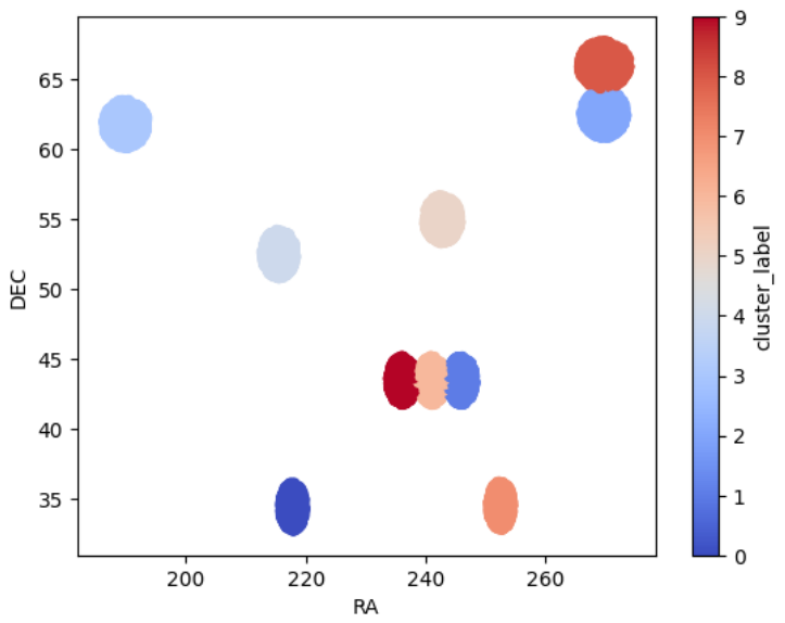
Visual inspection of the scatter plot of the RA and DEC suggested the presence of several broad sky partitions. To assign a label to each sample, the K-means algorithm was applied to the coordinate pairs. We emphasise that this should not be treated as a physical clustering analysis but rather as a pragmatic partition of the survey aimed at examining whether predictive performance varies systematically across the sky.

4.4.2. Quantitative Results

Figure 9 shows the spatial distribution of the samples colour-coded by their assigned cluster labels. Each colour indicates a distinct cluster identified by K-means. The cluster sizes are relatively balanced, with the largest cluster (label 5) comprising approximately 11.8% of all samples (

Table 13. Distribution of samples by cluster label assigned by K-means.

Cluster Label	Frequency	Proportion (%)
5	16,776	11.8
1	16,696	11.8
3	15,144	10.7
2	14,472	10.2
7	14,080	9.9
8	13,568	9.6
9	13,344	9.4
6	13,272	9.3
0	12,896	9.1
4	11,872	8.4

).

Table 14. $R^2$ scores for Z_MW by cluster label using KNN and MLP models: (a) AstroCLIP image embeddings and (b) AstroCLIP spectra embeddings.

(a)
Cluster Label	${\mathit{R}}_{\mathbf{KNN}}^{\mathbf{2}}$	${\mathit{R}}_{\mathbf{MLP}}^{\mathbf{2}}$
0	0.438	0.445
1	0.377	0.377
2	0.405	0.407
3	0.471	0.491
4	0.415	0.419
5	0.427	0.431
6	0.401	0.387
7	0.417	0.415
8	0.405	0.416
9	0.434	0.453
(b)
Cluster Label	${\mathit{R}}_{\mathbf{KNN}}^{\mathbf{2}}$	${\mathit{R}}_{\mathbf{MLP}}^{\mathbf{2}}$
0	0.584	0.641
1	0.523	0.593
2	0.555	0.608
3	0.601	0.640
4	0.573	0.622
5	0.561	0.615
6	0.571	0.613
7	0.581	0.630
8	0.536	0.586
9	0.621	0.669

presents the $R^2$ scores for $log\left(Z_{\mathrm{MW}}\right)$ across clusters for the KNN and MLP models using image and spectral embeddings.

For the image embeddings, $R^2$ varies moderately across sky partitions. The MLP model generally outperforms KNN and clusters 3 and 9 perform relatively well, whereas cluster 1 remains weak. For the spectral embeddings, the same broad pattern is visible, with the MLP again outperforming KNN across all partitions. We note that these differences should be interpreted cautiously. A sky position partition mixes many effects, including region-dependent differences, local observing conditions, and real astrophysical variation. Hence, the main value of the analysis in this section is the demonstration that performance is not perfectly uniform across the sky, which motivates the more targeted environment proxy analysis that follows.

4.5. Impact of Environment on Model Performance

This section investigates the relationship between local galaxy density and model performance. It outlines the methodology for estimating neighbour density, describes how galaxies were categorised into density bins, and reports the predictive accuracy of image- and spectrum-based models across these environmental conditions.

4.5.1. Experimental Setup

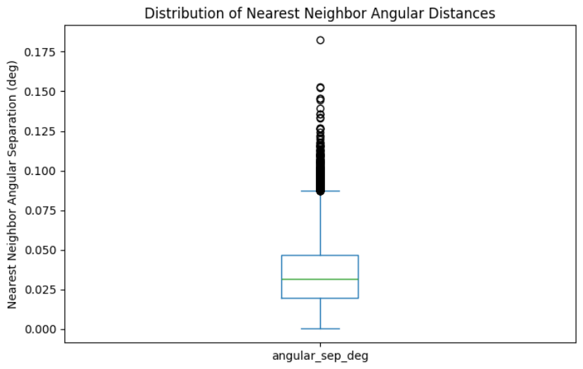
To quantify local density, the angular distance between each galaxy and its neighbours was calculated. Right ascension (RA) and declination (DEC) coordinates were transformed into sky positions and pairwise angular separations were computed while excluding self-matches. For each galaxy, the nearest-neighbour distance was recorded, resulting in a single scalar value per object. The distribution of these values is shown in Figure 10.

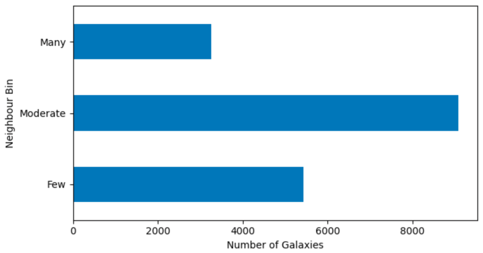
A threshold for the local neighbourhood distance was set as 1.5 times the interquartile range above the upper quartile of the nearest-neighbour distribution. A pairwise search was then conducted for all neighbours within this angular threshold. Each galaxy’s number of companions was counted and used as a proxy for local density. Based on this count, galaxies were grouped into three bins: few (up to three companions), moderate (four to seven companions), and many (more than seven companions). The bin-wise distribution is shown in Figure 11.

The use of angular neighbours makes this proxy straightforward to compute, but also introduces limitations. Most importantly, apparent crowding on the sky generally does not correspond to three-dimensional proximity, and redshift-space distortions can further complicate interpretation. Therefore, the results should be taken as showing how performance varies with this angular neighbour count and not as a three-dimensional characterisation of local environment.

4.5.2. Quantitative Results

The predictive performance of both KNN and MLP models was evaluated using $R^2$ across all neighbour bins for each property.

Table 15. $R^2$ scores for galaxy properties across neighbour bins for KNN and MLP models using image and spectra embeddings.

Embedding Type	Property	Neighbour Bin	KNN (${\mathit{R}}^2$)	MLP (${\mathit{R}}^2$)
Image	$log\left(M_{*}\right)$	Few	0.687	0.711
		Moderate	0.698	0.722
		Many	0.663	0.704
	$t_{age}$	Few	0.220	0.245
		Moderate	0.217	0.240
		Many	0.195	0.210
	$log\left(Z_{\mathrm{MW}}\right)$	Few	0.414	0.431
		Moderate	0.436	0.445
		Many	0.391	0.406
	$log\left(\mathrm{sSFR}\right)$	Few	0.313	0.367
		Moderate	0.346	0.403
		Many	0.339	0.386
Spectra	$log\left(M_{*}\right)$	Few	0.845	0.873
		Moderate	0.855	0.879
		Many	0.841	0.857
	$t_{age}$	Few	0.418	0.511
		Moderate	0.393	0.464
		Many	0.363	0.441
	$log\left(Z_{\mathrm{MW}}\right)$	Few	0.576	0.630
		Moderate	0.579	0.624
		Many	0.540	0.605
	$log\left(\mathrm{sSFR}\right)$	Few	0.580	0.647
		Moderate	0.618	0.674
		Many	0.625	0.683

reports results separately for models using image and spectrum embeddings.

For image embeddings, the moderate-density bin yields the strongest $R^2$ scores for three of the four targets. The MLP achieves its best results in this bin for $log\left(M_{*}\right)$, $log\left(Z_{\mathrm{MW}}\right)$, and $log\left(\mathrm{sSFR}\right)$. In contrast, performance in the many-neighbours bin is generally lower. The most obvious exception is $t_{age}$, for which the few-neighbours bin performs best. Spectral embeddings show a similar pattern. The best $log\left(M_{*}\right)$ performance again occurs in the moderate bin, whereas $log\left(\mathrm{sSFR}\right)$ increases toward the many-neighbours bin. For $t_{age}$, the strongest performance is found in the few-neighbours bin, consistent with the image-based results.

We briefly connect this to prior work which provides useful context for these findings. Stellar mass and star-formation history are known to vary with environment, and quenching processes are more common in denser regions [12,13]. Even so, our results do not provide direct evidence of those mechanisms because the environment measure here is only a neighbour-count proxy; thus, caution should be exercised. The conclusion we draw is a practical one, namely, that performance is not uniform across this proxy and is particularly good in regions that correspond to our intermediate-density bins.

4.6. Impact of Brightness on Model Performance

This section examines predictive performance across the two observational categories supplied by the released evaluation suite, namely, Low-z (Bright) and High-z (Faint). Given that redshift, apparent brightness, and signal-to-noise are entangled in flux-limited data, this split does not isolate brightness alone; instead, it provides insight into sensitivity to observational setting as a whole.

Quantitative Results

Table 16. $R^2$ scores by brightness category and property for KNN and MLP models using image and spectral embeddings.

Embedding	Property	Brightness Category	KNN (${\mathit{R}}^2$)	MLP (${\mathit{R}}^2$)
Image	$log\left(Z_{\mathrm{MW}}\right)$	High-z (Faint)	0.276	0.276
	$log\left(M_{*}\right)$	High-z (Faint)	0.606	0.630
	$t_{age}$	High-z (Faint)	0.120	0.150
	$log\left(\mathrm{sSFR}\right)$	High-z (Faint)	0.283	0.350
	$log\left(Z_{\mathrm{MW}}\right)$	Low-z (Bright)	0.510	0.527
	$log\left(M_{*}\right)$	Low-z (Bright)	0.733	0.775
	$t_{age}$	Low-z (Bright)	0.187	0.219
	$log\left(\mathrm{sSFR}\right)$	Low-z (Bright)	0.349	0.405
Spectra	$log\left(Z_{\mathrm{MW}}\right)$	High-z (Faint)	0.603	0.649
	$log\left(M_{*}\right)$	High-z (Faint)	0.867	0.888
	$t_{age}$	High-z (Faint)	0.305	0.366
	$log\left(\mathrm{sSFR}\right)$	High-z (Faint)	0.591	0.664
	$log\left(Z_{\mathrm{MW}}\right)$	Low-z (Bright)	0.515	0.578
	$log\left(M_{*}\right)$	Low-z (Bright)	0.817	0.863
	$t_{age}$	Low-z (Bright)	0.415	0.531
	$log\left(\mathrm{sSFR}\right)$	Low-z (Bright)	0.635	0.683

summarises the $R^2$ scores for the KNN and MLP models across brightness categories and embedding types. For image embeddings, the Low-z (Bright) group consistently achieves higher $R^2$ scores than the High-z (Faint) group for all properties. For example, metallicity improves from 0.276 to 0.510 for KNN and from 0.276 to 0.527 for MLP.

The difference in $R^2$ scores between categories is presented in

Table 17. $R^2$ score differences between the Bright and Faint categories for KNN and MLP models using image and spectral embeddings.

Embedding	Property	$\Delta {\mathit{R}}_{\mathbf{KNN}}^2$	$\Delta {\mathit{R}}_{\mathbf{MLP}}^2$
Image	$log\left(Z_{\mathrm{MW}}\right)$	0.234	0.251
	$log\left(M_{*}\right)$	0.127	0.145
	$t_{age}$	0.067	0.069
	$log\left(\mathrm{sSFR}\right)$	0.066	0.055
Spectra	$log\left(Z_{\mathrm{MW}}\right)$	0.090	0.070
	$log\left(M_{*}\right)$	0.050	0.030
	$t_{age}$	−0.110	−0.170
	$log\left(\mathrm{sSFR}\right)$	−0.040	−0.020

. For image embeddings, $log\left(Z_{\mathrm{MW}}\right)$ shows the largest gain, with improvements exceeding 0.23 for both models. Smaller but still notable gains appear for $log\left(M_{*}\right)$ and $log\left(\mathrm{sSFR}\right)$.

In contrast, the spectral embeddings do not show a uniform advantage for the Low-z (Bright) category. For $t_{\mathrm{age}}$ and $log\left(\mathrm{sSFR}\right)$, the High-z (Faint) subset even performs better. This finding suggests that the spectral representation is less sensitive than the image representation to this particular observational split for some targets.

These results resonate with what has been reported in previous work. The accuracy of metallicity predictions generally improves with higher signal-to-noise (S/N) data, which is often associated with brighter galaxies or can be improved through spectral stacking [14]. In spectral analysis, the precision of metallicity and age retrieval declines with lower S/N and improves with higher S/N [14]. Predictions of mass-weighted age and $log\left(\mathrm{sSFR}\right)$ from spectra also require adequate S/N [15]. Nevertheless, because the present split conflates S/N, redshift, and apparent brightness, it is not possible to attribute the observed performance differences to any one of these factors in isolation.

4.7. Residual Analysis for Image Embeddings

This section presents auxiliary investigations of residual behaviour for image embeddings in support of the comparative analyses presented in the previous section.

4.7.1. Experimental Setup

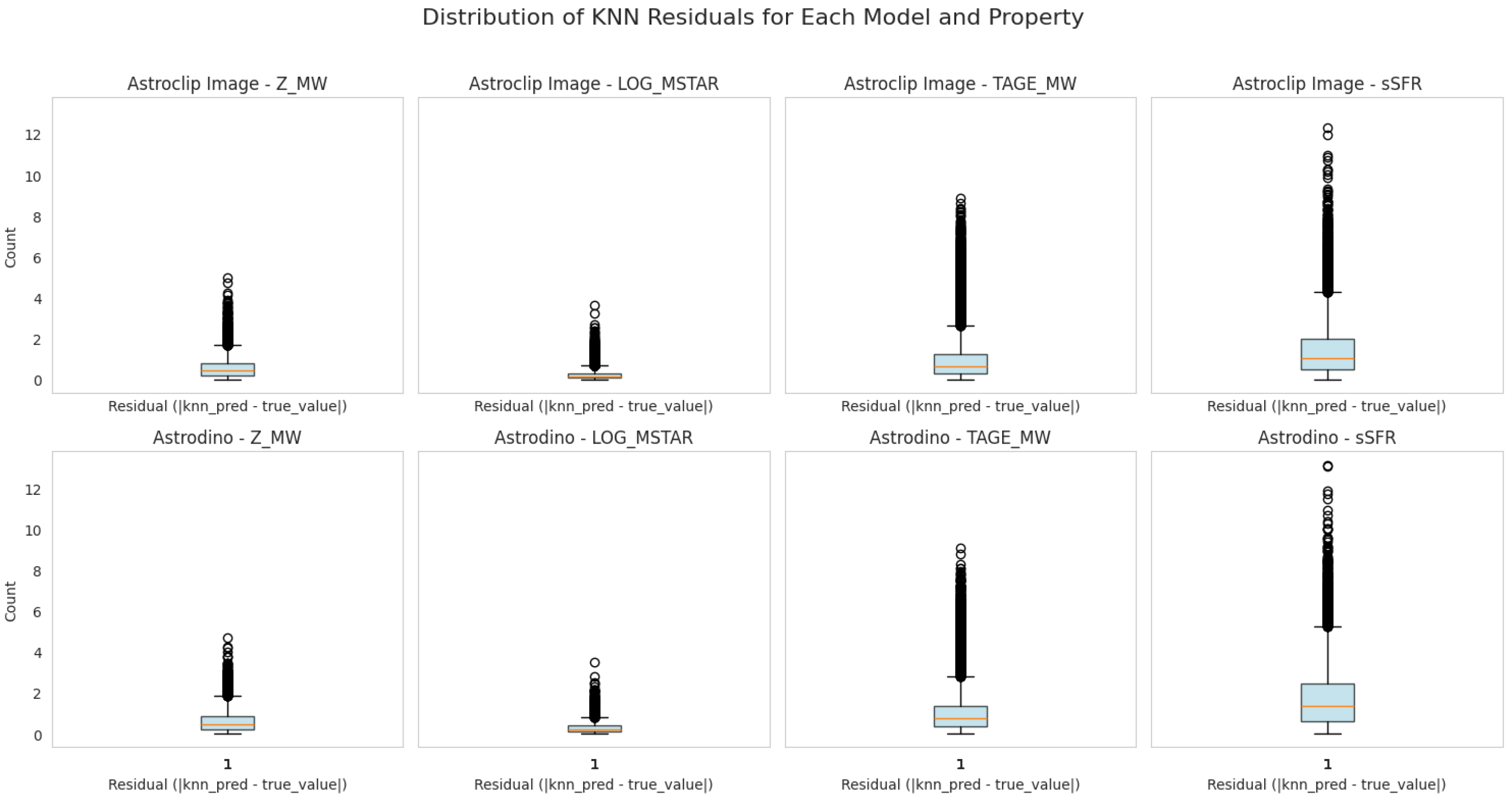
Residuals were computed for aligned and unaligned transformer models in order to determine whether the same input instances produced high errors across different configurations. For each predicted property, the element-wise absolute residual was calculated and the resulting distributions visualised using box plots. Outliers were identified according to the conventional criterion under which any residual greater than 1.5 times the interquartile range above the upper quartile is considered an outlier.

For comparative performance, each target variable’s range was divided into five quantile-based bins with equal population. For every data point, the prediction error was measured using the elementwise absolute value. The difference in residuals between the AstroCLIP and AstroDino models was computed for each instance. Within each bin, the net number of instances where AstroCLIP outperformed AstroDino was determined by subtracting the count where AstroDino had lower residuals. Histograms were constructed using the minimum description length (MDL) principle to select the optimal bin count. Figure 12 shows the distribution of absolute residuals for each model and property.

The procedure for MDL-based selection is detailed in Algorithm 1.

Outliers were examined to identify whether high residuals were shared between models or were property-specific.

Table 18. Distribution of outlier occurrence counts across properties for AstroDino and AstroCLIP.

Model	Outlier Count	Total	Proportion (%)
AstroDino	1	2308	82.55
	2	415	14.84
	3	65	2.32
	4	8	0.29
AstroCLIP	1	2464	79.13
	2	528	16.96
	3	112	3.60
	4	10	0.32

summarises the frequency of outlier occurrences. For AstroDino, 82.55% of outliers occurred only once, while AstroCLIP showed 79.13% single occurrences. This suggests that extreme residuals tend to be unique to specific properties rather than systematic across models.

Algorithm 1 Optimal histogram bin count via MDL

1: Input: Data array D, minimum bins $k_{min}$, maximum bins $k_{max}$    2: $N\leftarrow \left|D\right|$    3: ${\mathrm{best}}_k\leftarrow k_{min}$    4: ${\mathrm{MDL}}_{min}\leftarrow \infty$    5: for  $k=k_{min} \mathbf{to}$$k_{max}$  do    6:  Compute histogram: $c_i,e_i\leftarrow \mathrm{histogram}(D,k)$    7:  $p_i\leftarrow {\displaystyle \frac{c_i}{N}}$    8:  $p_i\leftarrow max(p_i,{10}^{-12})$    9:  $L_{\mathrm{data}}\leftarrow -{\sum }_{i=1}^k{c}_{i}log{p}_i$  10:  $L_{\mathrm{model}}\leftarrow {\displaystyle \frac{1}{2}}(k-1)logN$  11:  $\mathrm{MDL}\leftarrow L_{\mathrm{data}}+L_{\mathrm{model}}$  12:  if $\mathrm{MDL}<{\mathrm{MDL}}_{min}$ then  13:     ${\mathrm{MDL}}_{min}\leftarrow \mathrm{MDL}$  14:     ${\mathrm{best}}_k\leftarrow k$  15:  end if  16: end for  17: Return:  ${\mathrm{best}}_k$

4.7.2. Comparative Performance Across Property Bins

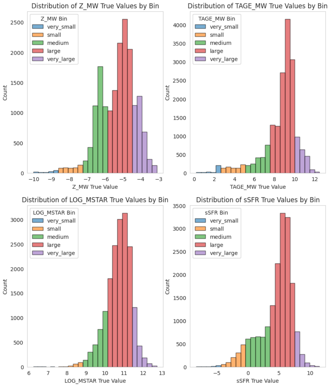
Figure 13 shows the distribution of each target property, coloured by quantile-based bins. This partitioning enables inspection of where each model performs better or worse.

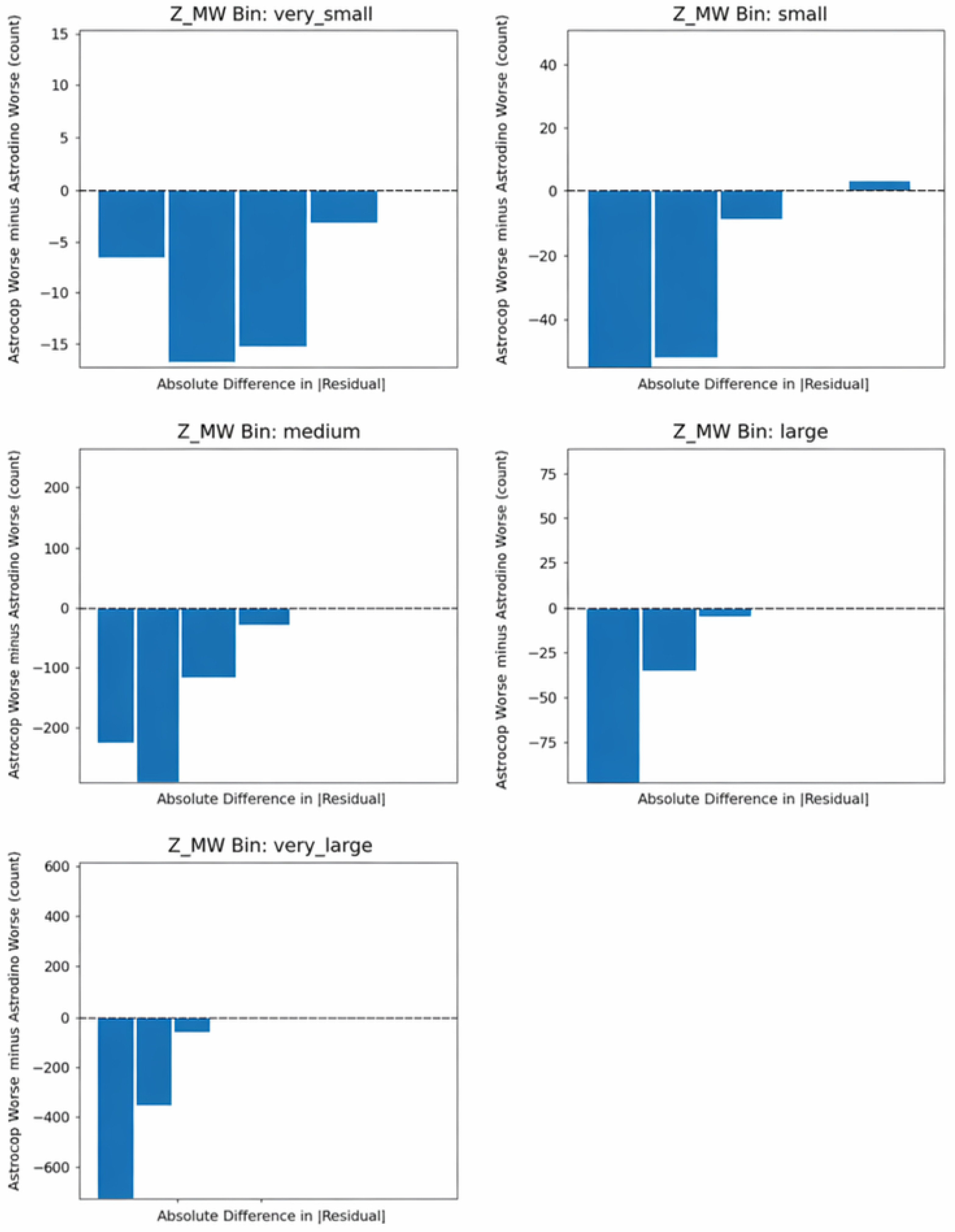
For $log\left(Z_{\mathrm{MW}}\right)$, Figure 14 illustrates the net instance counts by error magnitude. The medium and very large bins show consistently negative values across all error intervals.

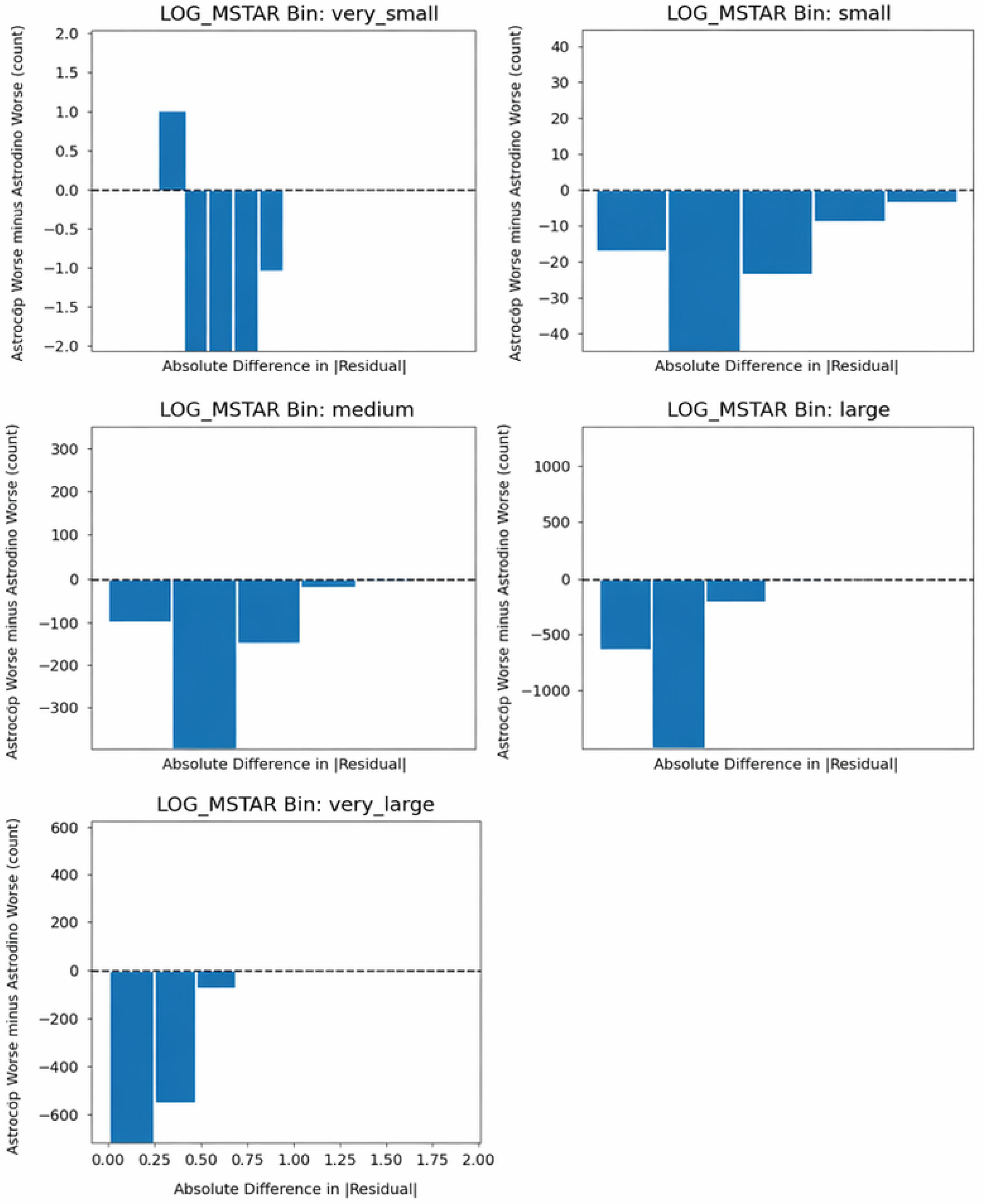
A similar pattern is observed for $log\left(M_{★}\right)$, as shown in Figure 15.

These results suggest that the performance differences between AstroCLIP and the image-based baseline are not confined to a narrow slice of the target range.

5. Discussion and Limitations

Our baseline reproduction confirms that spectral embeddings outperform image embeddings for the property estimation tasks considered here; furthermore, the robustness analyses we report show that performance is not uniform across observational or proxy-environmental settings. In addition, the embedding space analyses show that strong predictive performance does not require strong discrete cluster separation in low-dimensional projections.

We emphasise that low AMI values and weak UMAP separation do not imply that the embeddings are uninformative; instead, what they show is that a simple clustering of the embedding space aligns only weakly with discretised versions of single physical properties. Regression can still perform well if the relevant information is encoded continuously or if it is entangled with several properties. Accordingly, our clustering results should be understood as being limited by one specific style of interpretation, not as providing strong information about the downstream utility of a representation.

A number of limitations of the present work are also worth emphasising. First, our environment analysis relied on an angular neighbour-count proxy, and as such is vulnerable to projection effects, redshift-space distortions, and selection effects. Second, the adopted Low-z (Bright) versus High-z (Faint) split conflates redshift, apparent brightness, and signal-to-noise, which prevents clean attribution of observed differences to any one variable. Third, the few-shot results reported here are accompanied by bootstrap confidence intervals on test set predictions, but not by variability estimates across repeated training runs or alternative train/test splits. Finally, our analyses of UMAP and clustering should only be seen as heuristic tools for interrogating representation geometry and should not be taken as directly revealing the relevant physical structure.

6. Conclusions

In this paper, we have provided a careful reproduction of the released AstroCLIP regression benchmarks and extended them with stratified analyses across environment and observational splits. Our results help to interpret aggregate benchmark scores and highlight robustness patterns that were not examined in the original benchmark report.

We implement and analyse zero-shot and few-shot regression performance for $log\left(M_{*}\right)$, $log\left(Z_{\mathrm{MW}}\right)$, $t_{\mathrm{age}}$, and $log\left(\mathrm{sSFR}\right)$ using both galaxy images and spectra. Environmental and observational factors influencing model performance are also examined. While informative, the obtained results paint a nuanced picture requiring careful interpretation.

Our analysis reveals that spectral embeddings consistently outperform image embeddings across the regression tasks considered here, particularly in the zero-shot setting. AstroCLIP’s aligned spectral embeddings achieve $R^2$ values of 0.87 for $log\left(M_{*}\right)$, 0.57 for $log\left(Z_{\mathrm{MW}}\right)$, 0.43 for $t_{\mathrm{age}}$, and 0.63 for $log\left(\mathrm{sSFR}\right)$. Cross-modal alignment is most clearly beneficial in the image-based zero-shot setting, with the gains over the unaligned encoder being substantial for some targets. At the same time, the few-shot comparisons are mixed, and no strong conclusion should be drawn from them.

Our embedding space analysis shows that although UMAP visualisation reveals only weak clustering by individual physical properties, the learned representations can still support useful property estimation. K-means clustering on both image and spectral embeddings produces only weak agreement with discretised physical property bins, and HDBSCAN does not reveal stable and well-separated dense clusters under the tested settings. From this we conclude that the information carried by the embeddings is not well-captured by simple discrete clustering.

Environmental and observational factors have been found to affect model performance in a practically significant way. Under the neighbour-count proxy used, moderate-density environments often produce the strongest predictions for image embeddings, whereas spectral embeddings are somewhat more stable but still show systematic variation. The Low-z (Bright) versus High-z (Faint) split strongly affects image-based performance, while spectral embeddings appear comparatively less sensitive for some targets. Residual analysis suggests that the advantages of AstroCLIP over the image-based baseline are not confined to a narrow range of target values. Given that both robustness analyses rely on imperfect proxies or confounded splits, these findings do not support physical inferences but can be informative concerning practical use of the method.

Given that imaging surveys vastly outnumber spectroscopic observations, AstroCLIP’s ability to use scarce spectroscopic information to improve image-based representation learning addresses a real challenge in modern astronomy. Our work in this paper contributes both methodological and empirical value, shedding additional light on the model’s performance and limitations.

References

1. Parker, L.; Lanusse, F.; Golkar, S.; Sarra, L.; Cranmer, M.; Bietti, A.; Eickenberg, M.; Krawezik, G.; McCabe, M.; Morel, R.; et al. AstroCLIP: A cross-modal foundation model for galaxies. Mon. Not. R. Astron. Soc. 2024, 531, 4990–5011. [Google Scholar] [CrossRef]
2. Audenaert, J.; Bowles, M.; Boyd, B.M.; Chemaly, D.; Cherinka, B.; Ciucă, I.; Cranmer, M.; Do, A.; Grayling, M.; Hayes, E.E.; et al. The multimodal universe: Enabling large-scale machine learning with 100 TB of astronomical scientific data. In Advances in Neural Information Processing Systems; The MIT Press: Cambridge, MA, USA, 2024. [Google Scholar]
3. Dey, A.; Schlegel, D.J.; Lang, D.; Blum, R.; Burleigh, K.; Fan, X.; Findlay, J.R.; Finkbeiner, D.; Herrera, D.; Juneau, S.; et al. Overview of the DESI legacy imaging surveys. Astron. J. 2019, 157, 168. [Google Scholar] [CrossRef]
4. Walmsley, M.; Slijepcevic, I.V.; Bowles, M.; Scaife, A.M.M. Towards galaxy foundation models with hybrid contrastive learning. In Proceedings of the ICML Workshop on Machine Learning for Astrophysics, Baltimore, MD, USA, 17–23 July 2022. [Google Scholar]
5. Stein, G.; Blaum, J.; Harrington, P.; Medan, T.; Lukić, Z. Mining for strong gravitational lenses with self-supervised learning. Astrophys. J. 2022, 932, 107. [Google Scholar] [CrossRef]
6. Teimoorinia, H.; Archinuk, F.; Woo, J.; Shishehchi, S.; Bluck, A.F. Mapping the diversity of galaxy spectra with deep unsupervised machine learning. Astron. J. 2022, 163, 71. [Google Scholar] [CrossRef]
7. Melchior, P.; Liang, Y.; Hahn, C.; Goulding, A. Autoencoding galaxy spectra. I. Architecture. Astron. J. 2023, 166, 74. [Google Scholar]
8. Hayat, M.A.; Stein, G.; Harrington, P.; Lukić, Z.; Mustafa, M. Self-supervised representation learning for astronomical images. Astrophys. J. Lett. 2021, 911, L33. [Google Scholar] [CrossRef]
9. Liang, Y.; Melchior, P.; Lu, S.; Goulding, A.; Ward, C. Autoencoding galaxy spectra. II. Redshift invariance and outlier detection. Astron. J. 2023, 166, 75. [Google Scholar] [CrossRef] [PubMed]
10. van der Vaart, A.; Bijma, F.; Jonker, M. Regression models. In An Introduction to Mathematical Statistics; Amsterdam University Press: Amsterdam, The Netherlands, 2017; Chapter 7. [Google Scholar]
11. Vinh, N.X.; Epps, J.; Bailey, J. Information theoretic measures for clusterings comparison: Is a correction for chance necessary? In Proceedings of the 26th Annual International Conference on Machine Learning, Montreal, QC, Canada, 14–18 June 2009. [Google Scholar]
12. Kauffmann, G.; White, S.D.; Heckman, T.M.; Ménard, B.; Brinchmann, J.; Charlot, S.; Tremonti, C.; Brinkmann, J. The environmental dependence of the relations between stellar mass, structure, star formation and nuclear activity in galaxies. Mon. Not. R. Astron. Soc. 2004, 353, 713–731. [Google Scholar] [CrossRef]
13. Sol Alonso, M.; Lambas, D.G.; Tissera, P.; Coldwell, G. Effects of galaxy interactions in different environments. Mon. Not. R. Astron. Soc. 2006, 367, 1029–1038. [Google Scholar] [CrossRef]
14. Citro, A.; Pozzetti, L.; Moresco, M.; Cimatti, A. Inferring the star-formation histories of the most massive and passive early-type galaxies at z < 0.3. Astron. Astrophys. 2016, 592, A19. [Google Scholar]
15. Cohn, J.D. Approximations to galaxy star formation rate histories: Properties and uses of two examples. Mon. Not. R. Astron. Soc. 2018, 478, 2291–2314. [Google Scholar] [CrossRef]
Figure 1. Example galaxy images from DESI-LS [3].
Information 17 00422 g001
Figure 2. Example optical spectra from DESI [2].
Information 17 00422 g002
Figure 3. Two-dimensional UMAP projections of aligned image embeddings. Galaxies are coloured by binned physical properties. Each panel represents a distinct property with values divided into low and high categories.
Information 17 00422 g003
Figure 4. Two-dimensional UMAP projections of unaligned image embeddings. Galaxies are coloured by binned physical properties. Each panel represents a distinct property with values divided into low and high categories.
Information 17 00422 g004
Figure 5. Two-dimensional UMAP projections of aligned spectrum embeddings. Galaxies are coloured by binned physical properties. Each panel represents a distinct property with values divided into low and high categories.
Information 17 00422 g005
Figure 6. Two-dimensional UMAP projections of unaligned spectrum embeddings. Galaxies are coloured by binned physical properties. Each panel represents a distinct property with values divided into low and high categories.
Information 17 00422 g006
Figure 7. Elbow curves for K-means clustering of AstroDino (left) and AstroCLIP (right) image embeddings. Inertia is plotted against the number of clusters k. The dotted red lines correspond to the selected value k = 3 .
Information 17 00422 g007
Figure 8. Elbow curves for K-means clustering of SpecFormer (left) and AstroCLIP spectral embeddings (right). The dotted red lines correspond to the selected value k = 3 .
Information 17 00422 g008
Figure 9. Scatter plot of sample coordinates (RA, DEC) colour-coded by cluster label as determined by K-means clustering.
Information 17 00422 g009
Figure 10. Box plot of nearest-neighbour angular distances, illustrating the spread of local separations across the galaxy sample.
Information 17 00422 g010
Figure 11. Distribution of galaxies across neighbour bins, defined by the number of companions within the angular distance threshold.
Information 17 00422 g011
Figure 12. Box plot of the absolute residuals for each model and property using KNN.
Information 17 00422 g012
Figure 13. Distribution of target variable values with quantile-based bin membership.
Information 17 00422 g013
Figure 14. Net instance count by error magnitude where AstroCLIP outperformed (negative values) or underperformed (positive values) AstroDino for log ( Z MW ) , shown by target-value bins.
Information 17 00422 g014
Figure 15. Net instance count by error magnitude where AstroCLIP outperformed or underperformed AstroDino for log ( M ) , by target-value bins.
Information 17 00422 g015