Article

Data-Driven Reconstruction of the Singapore Stone: A Numerical Imputation Method of Epigraphic Restoration

by
Tehreem Zahra
1,*,
Francesco Perono Cacciafoco
2,* and
Muhammad Tayyab Zamir
3
1
Independent Researcher, Shah Faisal Colony, Multan 60000, Pakistan
2
Department of Applied Linguistics, Xi’an Jiaotong-Liverpool University, Suzhou 215123, China
3
Centro de Investigación en Computación, Instituto Politécnico Nacional, Ciudad de México 07700, Mexico
*
Authors to whom correspondence should be addressed.
Information 2026, 17(2), 170; https://doi.org/10.3390/info17020170
Submission received: 10 December 2025 / Revised: 26 January 2026 / Accepted: 26 January 2026 / Published: 7 February 2026

Abstract

One of the key artefacts of epigraphy in Southeast Asia is the Singapore Stone inscription, which is, unfortunately, in a poor condition. There are huge spaces that separate the readable characters, rendering the text incomplete. This renders a traditional reconstruction and interpretation by philologists extremely challenging. We consider epigraphic restoration as a data-restoration task in this paper. We represent the inscription as a system of categorical symbols, in keeping with the original spatial disposition of characters and spaces. Our model is trained in a conservative, data-driven manner using the observed symbols to learn the local transition statistics, and it takes advantage of this information to make plausible predictions of the most likely characters in missing sequences that are short and well-constrained. The procedure generates a probabilistic hypothesis of restoration, which can be audited, as opposed to one definitive reading. The validation of masked-character recovery demonstrates that the model has a mean top-one error of 53.3%, which represents a significantly worse performance compared with simple baseline methods. The process is focused on interaction and transparency with experts. It relies upon assurance scores and prioritised alternative completions of each proposed reconstruction, as a useful means to produce hypotheses in computational epigraphy and the digital humanities.

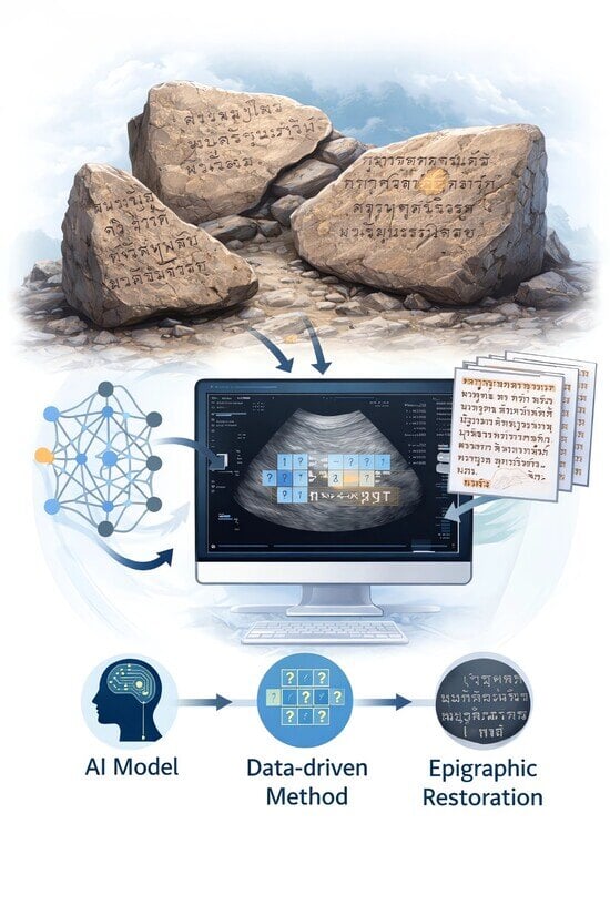
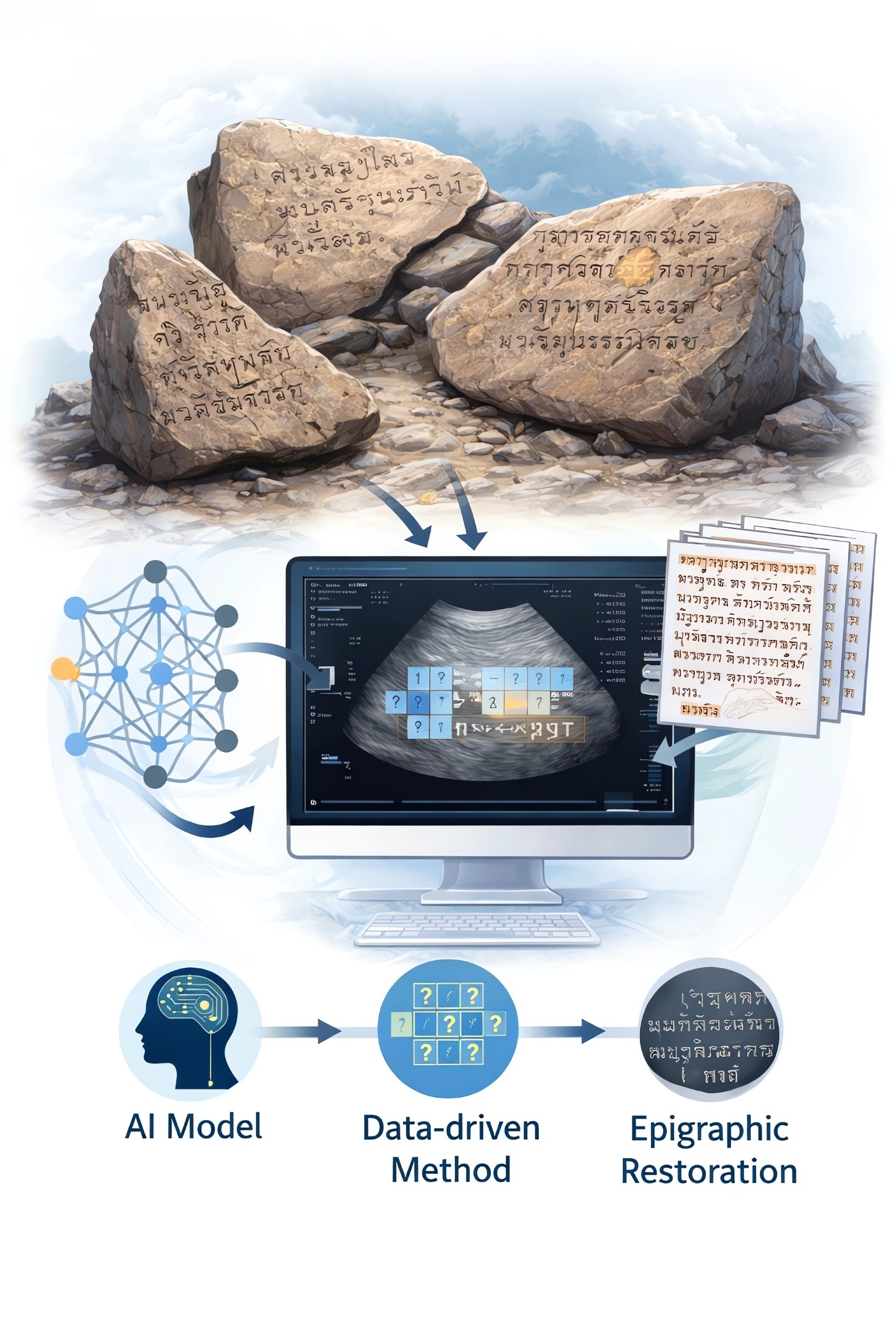
Graphical Abstract

1. Introduction

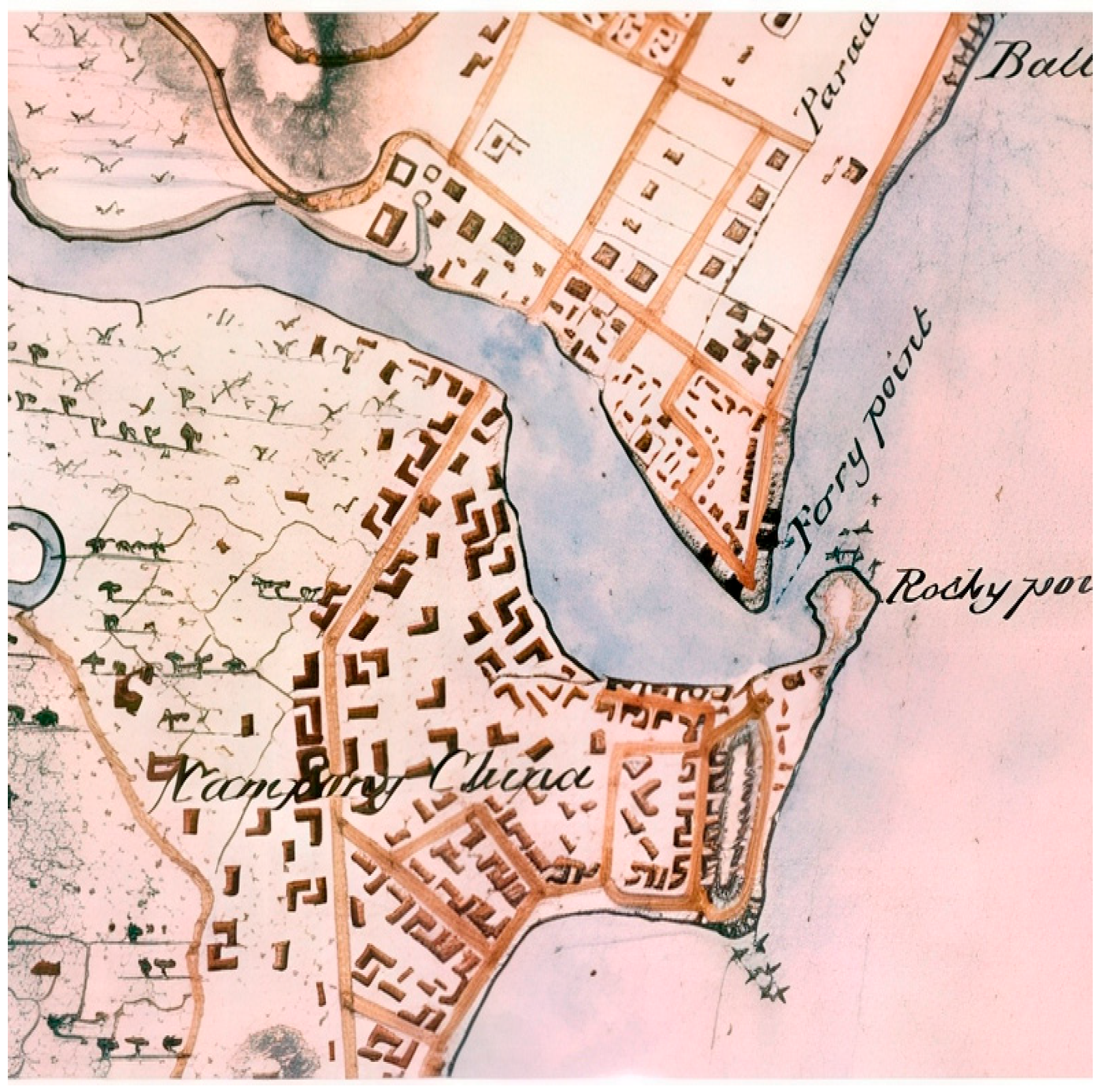
The Singapore Stone, which is a piece of monolithic sandstone, was initially discovered in 1819. Figure 1 shows that the initial location of the monolith was at the mouth of the Singapore River. The inscription is still regarded as one of the most crucial and unrelenting epigraphic mysteries in Southeast Asia [1].
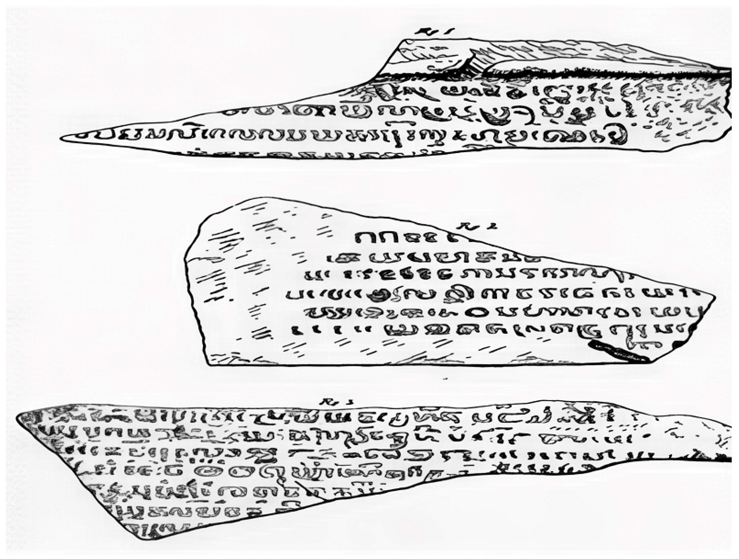
The monument is connected with the maritime trade history of ancient Temasik, which was a fourteenth-century port city [2,3]. Temasik participated in broader regional economic and cultural networks [2,3]. The memory of the Stone is also kept alive in the local folklore. The legend of the strongman Badang, which appears in the Sejarah Melayu (Malay Annals), tells that he dropped a very big rock into the river [4,5]. In 1843, the Stone met its irreparable loss, when British engineers caused the explosion to make an opening to Fort Fullerton. This blew the monument to pieces (Figure 2) [1,6]. The artefact that remained is housed in the National Museum of Singapore as a national treasure. It still reminds us of what has been lost and of the intellectual challenge that the inscription poses [7,8].
This speculation has lasted for two hundred years, and efforts to decipher the inscription have given more guesses than answers. This made the eroded surface of the script a hindrance to early work. Sir Stamford Raffles and Dr William Bland drew an incorrect conclusion on this matter, suggesting that the script was Pali [9,10]. Subsequently, theories of Tamil influence have been proposed (1834), such as those of Captain Peter James Begbies, who preceded the modern view that the writing is that of the Later Kawi school [11,12]. Nevertheless, there is a complicated history of this consensus. There is a scholarly dispute on the language used in the inscription, whether it is Old Javanese or Sanskrit. Even the diacritics are remarkably small, and thus hard to read in the Brahmic family of writing [6,13]. This interpretive stalemate shows a significant gap in the research. Computational methods may assist scientists to overcome the constraints of the traditional palaeographic analysis [1,14].
The physical history of the fragments is also complicated. After the destruction of the stone in 1843, some of the inscribed pieces were saved. They were deposited in the Museum of the Royal Asiatic Society in Calcutta (since renamed the Indian Museum) to be studied by Lieutenant-Colonel James Low [1,15,16]. The works were left for decades in Calcutta. It is also suspected that much of the Stone was cut in Singapore into gravel, which further diluted the corpus [6]. One piece was returned in 1918, which weighed 80 kg and measured 67 cm, and it is currently known as the Singapore Stone [6,17]. The rest of the pieces are believed to be in Calcutta, but their location is uncertain. This also endows the surviving text with even greater significance as it is the primary source of information [1].
Figure 2. As reported by [18]. The three fragments of the Singapore stone.
Information 17 00170 g002
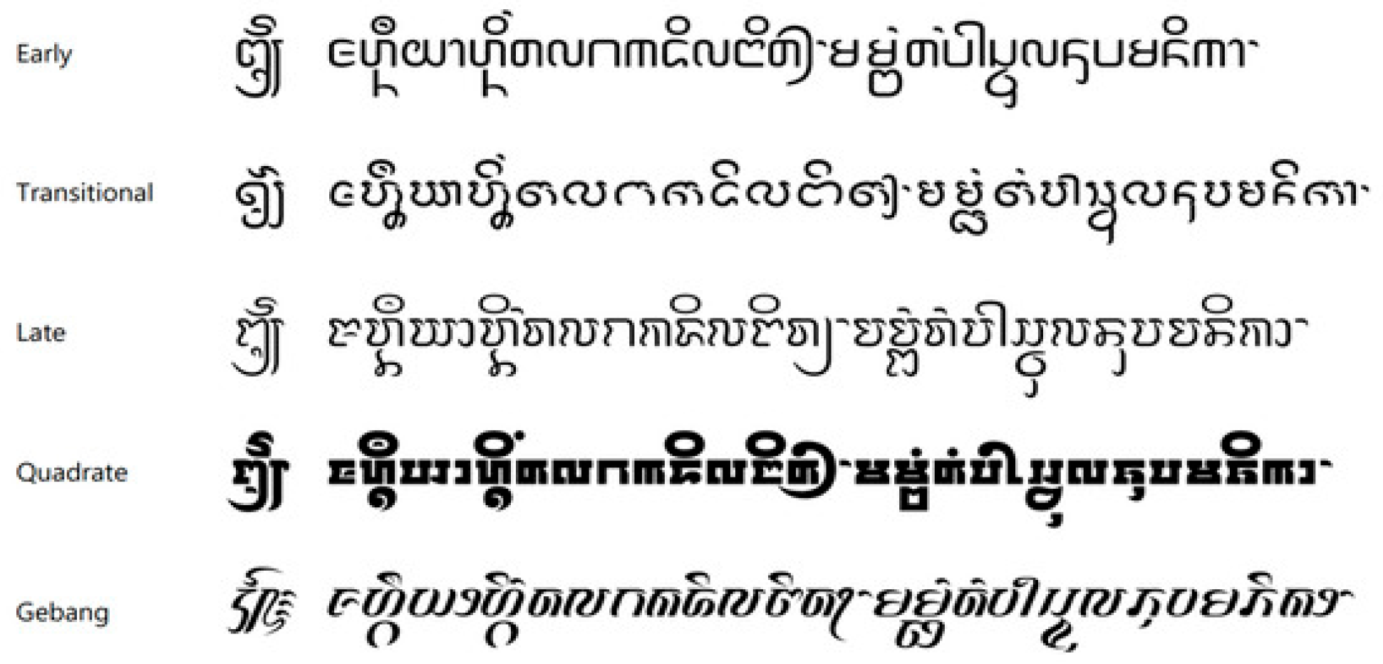
The script itself is the most detailed contemporary investigation, which assigns the script to Later Kabi (Figure 3). Lee and Perono Cacciafoco facilitate this classification with a long comparison with the Calcutta Stone, which is an inscription dated 1041 CE [12,13]. The two inscriptions have a lot of similar characters, which justifies that they be grouped together. Nevertheless, Lee and Perono Cacciafoco also give an aberration. Singapore Stone contains an abnormally low ratio of diacritics and clusters of characters. This is uncharacteristic of Kawi traditions, and it makes it directly more difficult to decipher [13,18]. The fact that the Stone is fractured contributes to this issue. It constrains our possibility to define ancient vowels of writing and the arrangement of syllables in Brahmic scripts. Considering these challenges, we promote computational and data-driven methods, which are capable of suggesting plausible reconstructions, rather than analyses.
A major gap in the literature is covered in this paper, which re-defines epigraphic restoration as a missing-data problem. We symbolise each of the surviving graphemes by a compact categorical ID, and we also make a note of every piece of lost text as a quantifiable number of character spaces. This representation maintains the locality of space of the inscription to be computed. The statistics are very scanty. Due to that reason, reconstruction is local and conservative. Our model is a smoothed first-order Markov transition model (bigram probabilities) that is trained on the observed immediately preceding IDs. We will then only propose reconstructions of short bounded internal gaps (contiguous NaN between observed IDs), restricted by a maximum length K (in a similar case, K = 5). Viterbi bridging is used to calculate the most probable completion of any viable gap. The next step is to estimate ambiguity with posterior marginals of a forward/back pass. We give such results as confidence scores and ordered sequences of alternatives. The proposed fillings can then be replicated by specialists in the form of grapheme exemplars to be inspected. This makes the workflow a process that can be repeated, not an automatic system of decipherment.
The restoration of texts and graphics is not easy. The Singapore Stone is difficult to read since the remaining piece of text is fragmented and unfinished. The initial monolith was lost and disintegrated, and it lacks sufficient philological data on which morphology and syntax can be rebuilt with confidence [1]. The dating of the writing to the Later Kawi school is supported by most palaeographers. There are, however, a number of atypical characteristics that make phonological and linguistic interpretation difficult. The fact that there are relatively few diacritics in the script is one problem [13], and the context of the archaeological background is another. The inscription is in a current condition, indicating the disturbance of time and imbalanced conservation. Any reconstruction suggested must then be clear of doubt, and it must not give speculation under the guise of being recovered text.
On a broader level, Southeast Asian palaeographic surveys indicate that Kawi and related Brahmic scripts are characterised by the organisation of grapheme inventories and localised patterned sequences. Even strands of strings, which are heavily damaged, may still have short-range regularities, with no translation necessary. The gaps and editorial interventions are already explicitly coded in the practice of digital humanities. They are treated by editors as objects, as opposed to muting omissions. This is common to epigraphic encoding and TEI/EpiDoc in particular [19]. The text may also be put into the perspective of missing-data inference [20] and the contemporary practice of imputation. Such methods put a strong focus on careful guesses and clear statements about uncertainty, such as in the case of gap marks that are regarded as a direct missing value [21,22]. Our approach to this concept is probabilistic sequence modelling. We infer the first-order transition structure using the observed adjacencies; then, we compute bounded-gap completions on the basis of dynamic programming. Instead of a single opaque answer, this workflow generates ranked and confidence-tagged restoration hypotheses [23,24].

2. Literature Review

The Singapore Stone holds a special position in the epigraphy of Singapore. The discussion of its archaeology, identification of its language and script, and its cultural significance are the typical areas of focus in the literature. The Stone is located in the social and economic organisation of the fourteenth-century Temasik by the researchers. The development of this context was done by Heng [2]. According to Yap, Jiao and Perono Cacciafoco, the portions were rediscovered in 1819, destroyed in 1843, and dispersed later [1]. They also examine initial suggestions of Tamil or Pali descent and the present opinion that the writing was Later Kawi [1]. They also write about decolonisation and cultural repatriation in their work, referring to the Rosetta Stone. In a comparative study, Lee and Perono Cacciafoco justify the Later Kawi classification using the Calcutta Stone [13]. The few diacritics, however, make it difficult to interpret. There is still controversy about the language of the inscription, which could be either Old Javanese or Sanskrit. This ambiguity cannot be resolved by comparing it with the corpus of Old Malay inscriptions that was compiled by Griffiths [25].
This deadlock represents general problems in the use of inscriptions to reinforce identity and place-making. Yeoh [26], in his example, talks about toponymic inscriptions and nation-building, and demonstrates how physical landscapes may imply an ideology. The boundaries of traditional epigraphy of eroded or broken artefacts can also be seen in the earlier methods of recording. Bland employed the use of dough impressions, and Laidlay employed the use of charcoal rubbings [15]. Subsequent studies of multiracialism [27], the dialect frontier [28], consumer capitalism [29,30], and heritage structures [26] also indicate that the politics of contemporary culture can be used to influence interpretative attitudes. The comparative palaeography and the inscription catalogues, including a systematic one by Griffiths [25], are still helpful. Nevertheless, the anomalies of the Singapore Stone, including its low diacritic frequency, require other approaches. This encourages us to use the missing-data modelling and multivariate imputation of numerically encoded grapheme sequences. It seeks to find out the trends and suggest plausible reconstructions beyond the constraints of the orthodox epigraphic practice.

3. Materials and Methods

3.1. Source Material and Scope

The sequencing workflow generates hypotheses about the Singapore Stone inscription. We use a conservative, verifiable methodology based on a line-by-line transcription from the available visual evidence, including a lithograph and photographs of the surviving fragments. The procedure addresses two questions: first, which local completions are suggested by observed adjacency patterns? Second, how conjectural is each computational suggestion?

3.2. Grapheme Encoding

Each grapheme identified in the transcription receives an ID. The IDs are nominal categories, and they do not encode phonetic values, palaeographic features, or numerical order. We store the mapping between each ID and its graphemic form as a project codebook, and we treat it as research data. ID-based encoding enables reproducible computation without special fonts, and it also keeps the modelling stage independent of disputed linguistic interpretations. Later linguistic analysis can still use the codebook, but the reconstruction model only recognises categorical states.

3.3. Gap Measure Position-Preserving Line Representation

To preserve geometry, we store each of the 32 inscription lines as a short string. The string interleaves observed IDs with explicit gap declarations of the form “(N character spaces)”. Here, N approximates the number of missing character slots. We estimate gap lengths by measuring the space between readable characters in the same observation. We use uniform measurements of average character width and spacing, so that one empty slot corresponds to one potential character position. A gap declaration, therefore, marks unread material, not an orthographic word space. This representation keeps a stable position index along each line. It allows us to compare positions, quantify missingness, and identify the exact locations where the algorithm proposes restorations.

3.4. Decomposing Where Values Are Missing in Arrays

We convert line strings into numerical arrays with a deterministic parser, parse-line-preserve-positions. A regular expression tokenises each line into either a gap token (“(N character spaces)”) or a numeric token (an observed ID). For a gap token, the parser reads N and inserts Not-a-Number (NaN) values at the corresponding positions. For a numeric token, the parser casts the ID to a number and appends it. The output for each line is a one-dimensional NumPy 2.4.2 array. Observed positions contain numeric IDs, and missing positions contain NaN. Line lengths vary, so we store the result as a list of arrays. For matrix-based reporting, we pad each array to the maximum line length (219 positions). We also create a validity mask so that padding is never treated as part of the inscription.

3.5. Learning a Categorical Transition Model

The integers (IDs) are categorical symbols. The reconstruction model must not treat them as numbers with an order. We use a first-order Markov model, also called a bigram model, and we only train it on observed adjacent pairs in the encoded inscription.
The model is built as follows:
We scan the inscription line by line. We count each transition from the symbol at position i to the symbol at position i + 1. We only count a transition when both symbols are observed (i.e., neither is missing/NaN).
Let:
  • C(a,b) = the count of observed transitions from symbol a to symbol b
  • C(a) = ∑b C(a,b) = the total number of observed outgoing transitions from symbol a
  • V = the total number of unique observed symbol IDs
  • α = an additive smoothing parameter (set here to α = 0.5)
Because the dataset is sparse, many plausible transitions are not directly observed. To avoid zero-probability transitions, we apply additive smoothing. The transition probability from symbol a to symbol b is estimated as
P(b∣a) = (C(a) + α V)/(C(a,b) + α)
For any symbol a that has no observed outgoing transitions (i.e., C(a) = 0), the model assigns a uniform probability distribution across all V possible symbols.
Finally, we store the transition probabilities in a V × V matrix T. For numerical stability in the dynamic programming steps, we also compute log T, the element-wise logarithm of T.

3.6. Gap Taxonomy and Conservative Eligibility Regulations

An internal gap is a continuous run of NaNs that is preceded and followed by observed IDs in the same line. A lacuna can be unbounded. It has only one anchor, or no anchors at all. This can occur at the start or end of a line, or in long damaged regions where only one side is readable.
We fill bounded gaps only, because they define a well-posed local bridging problem with evidence on both sides. To avoid speculative long-range completion, we set a maximum eligible gap length K. In our initial setting, K = 5. We therefore fill only bounded gaps with lengths from 1 to 5. We leave longer bounded gaps and all unbounded lacunae unfilled. This policy reflects a methodological decision to prioritise interpretability and auditability over visual completeness.

3.7. Viterbi Bridging and Maximum a Posteriori Completion

We infer an ID sequence x1…xL that maximises the bridge probability in the transition model for each eligible bounded gap of length L. The gap has a left endpoint symbol ℓ and a right endpoint symbol r. The log score of a candidate sequence is computed as
log Pf(x1ell) + sum t = 2 to L log Pf(xtx 1(t − 1)) + log Pf(rxlxL).
This provides an accurate calculation of the maximum a posteriori sequence. We use Viterbi-style dynamic programming on the V categorical states. The algorithm represents the best log score of any path ending in state j at each gap position t and state j. It also stores a back-pointer to the previous state that attained such a score. We introduce the jump into R and unwind the pointers and recover the optimum sequence. The blank IDs are substituted with recovered IDs, and the occurrence of gaps in the line array is filled. This deterministic inference has a computational size that is small since L is limited by K.

3.8. Confidence Scores and Posterior Marginal

The optimal order does not represent certainty. The pipeline thus solves the posterior marginals of the IDs in every gap position, assuming that the boundaries are fixed. Assuming that L is the length of a gap, we compute backwards and forwards an equal run of the same Markov chain. The forward values are the sum of the log probabilities up to the left endpoint symbol ℓ to every internal position. The backward values are the accumulation of log probabilities in each internal position to r. The values are added together to form an unnormalised score of every state and normalised using a log-sum-exp operation. We report a transparent confidence score of log (p1/p2) to each position, where we take the two most likely posterior probabilities p1 and p2.
A small value indicates that the best candidates are very close to each other. A higher value implies that there is a clear preference of the best candidate. Each slot that is filled is given a confidence score. We also collectively summarise the gaps in terms of their mean and minimum confidence. This assists the users to concentrate on more strongly locally evidenced suggestions.

3.9. Computer-Generated Variants: The Five Optimal Exact Candidate Sequences

The workflow provides a list of alternative restorations to use to fill in each gap filled. This facilitates professional comparison. The k-best dynamic programming algorithm is used to compute the five best bridge sequences. The single best path is not the only propagated path; at each end state and position, the algorithm propagates the best k paths. We sort the sequence of candidates based on the sum of their log probabilities. In order to simplify the interpretation of the results, we normalise probabilities in the set of the top five displayed. The corresponding relative probabilities are then added to the gap. We give out these outputs as gap-level rankings, and not as absolute chances of being right. It is hoped that this eliminates ambiguity, rather than hide it.

3.10. Masked-Character Recovery and Baseline Validity

Masked-character recovery with known material is applied to quantitative validation. The eligibility criteria of a site are that it is an observed ID and both its immediate right and left neighbours are observed. This makes the evaluation the same as the limited gap task. In 50 repetitions, 15 percent of qualified sites in one line are masked. The masked sites are not adjacent, meaning that every target is a single isolated slot. On each masked site with neighbours 1 and r, the model computes the missing ID × by maximising the local bridge score P(x|ell)P(r). Two baselines are also calculated. The most frequently observed ID in the corpus is always predicted by a mode baseline. ID is sampled at random in the empirical unigram distribution with a frequency-matched random baseline. These criteria distinguish actual context sensitivity and the influences of the general frequencies of symbols.

3.11. Invariance Tests, Calibration of Confidence, and Sensitivity Tests

The hypothesis that the confidence is correlated with the correctness is tested with the help of computation of the confidence of each masked prediction and binning of the predictions into five equal-sized confidence strata. The result of empirical accuracy divided by stratum is used to create a calibration plot that conveys the behaviour of confidence in practice. Given that the labelled IDs are categorical, we also carry out a test of invariance: the labels are randomly permuted, the pipeline is used on permuted labels, and the predictions are reversed to permuted labels. This is because re-labelling invariance is a direct test that the algorithm is not based on some accidental numerical ordering. Finally, hyperparameter sensitivity is recorded by varying K and α and the logged results are the completion coverage and accuracy of masked characters at these parameters.

3.12. An Example of Algorithmic Repair

Position maps encode all cells as seen, retain lacunae, and input and use the validity mask to remove padding artefacts. Other elements are the holdout accuracy, confidence calibration, gap length distribution, and the profile of sparsity with the line width. To provide a graphical representation of the algorithmic repair of the lithograph, the workflow renders a before-and-after panel, which identifies the same relative locations of the bounded gaps, and only the slots that are predicted by the algorithm are rendered. The contents that are inserted are based on the project codebook, such as the related grapheme exemplar or their trace, and are graphically differentiated by colour coding relative to the background. This guarantees that the demonstration represents algorithmic suggestions with no transformation of the basic witness image.

4. Results and Discussion

The independent reproducible pipeline is used to compute all the results in this section using the same position-preserving dataset. The 32 inscription lines are coded in a one-dimensional array of grapheme IDs in the form of categorical representations. The exact number (N character spaces) of segments is multiplied by the exact Not-a-Number (NaN) so that the digital representation does not reduce the original spatial structure and gaps between gaps to a single continuous string. Due to the sparsity of the dataset, which is very intense, the discussion is made with deliberate caution: the workflow is presented to the expert with the hypothesis generator, rather than as an automatic decipherment system.

4.1. Coverage of Data and Conservative Restoration

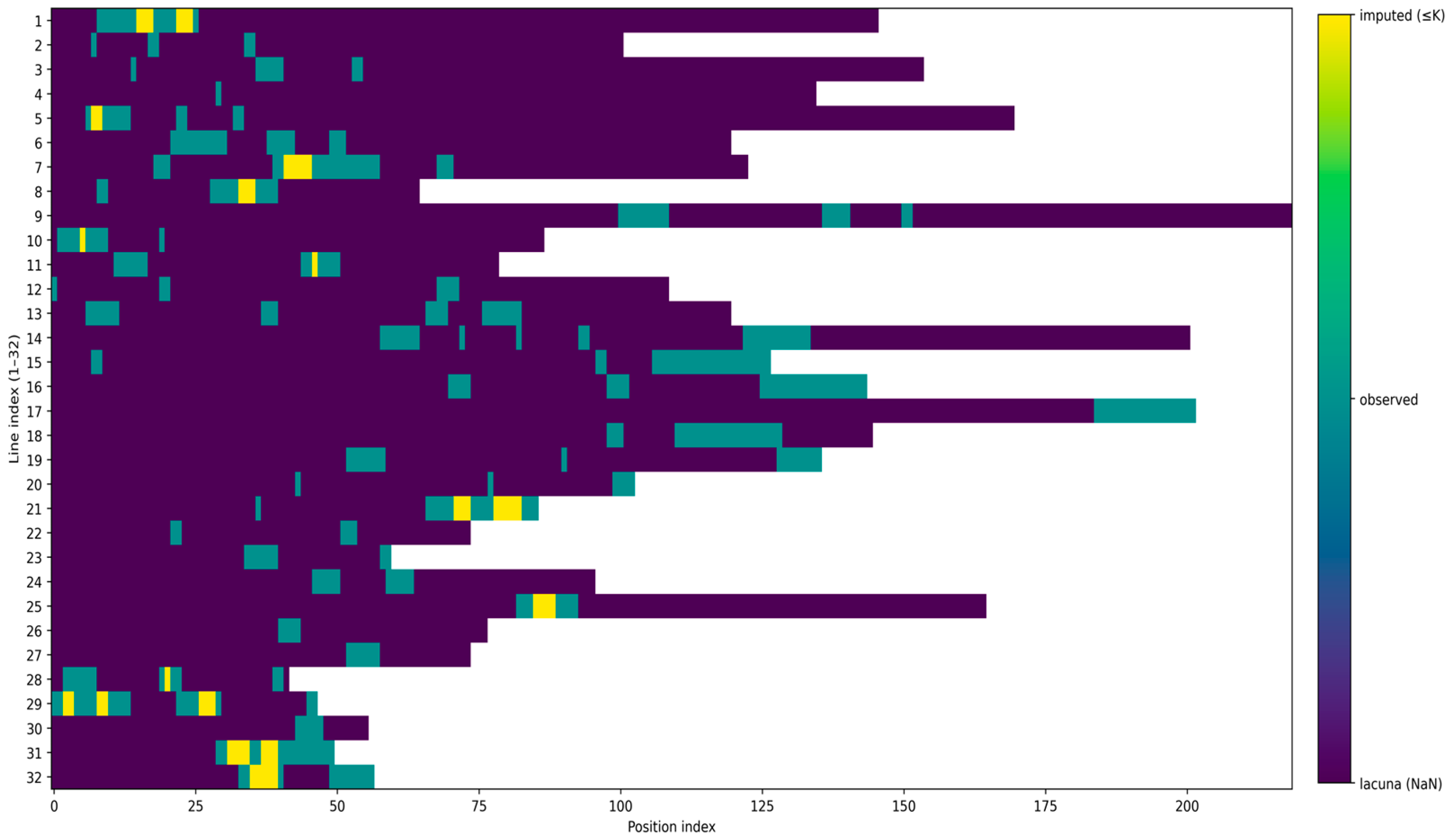
When all the lines have been parsed, the encoded matrix has 3570 positional slots (maximum line width 219). It only has 397 slots that have seen grapheme IDs (11.1 coverage), and 3173 slots (88.9 absence) are not present. There is not one uniform lack, there are many long initial gaps at the beginning of the lines, and many long final gaps at the end of the lines, and these are suggestive of the habits of physical loss in the record now extant.
So as not to exaggerate, we distinguish two kinds of missing segments, including the internal gap. This is a continuous NaN run that is immediately followed by observed IDs and immediately preceded by observed IDs in the same line. Any run of NaN which has no left or right boundary, or both (as often occurs at the ends of a line or in vast destroyed regions), is known as the unbounded lacuna. There are 111 NaN runs in total in the current dataset, 59 bounded internal gaps (843 missing positions) and 52 unbounded lacunae (2330 missing positions). Bounded internal gaps are only localizable through being completed as they have immediate contextual anchors on each side.
Long spans, even between limited gaps, suggest speculation. We thus use a definite length threshold K, which only allows completion of short gaps. The K in the setup mentioned in Figure 4, Figure 5, Figure 6, Figure 7, Figure 8, Figure 9 and Figure 10 will be 5, i.e., only bounded gaps with a length less than 5 will be considered. Within the given conservative environment, 17 bounded gaps are admissible and 50 positions are simulated. All the other missing positions—793 bounded gaps greater than five and 2330 of the unbounded positions—are still missing. This is a major characteristic of interpretability. When the method exclusively focuses on small discontinuities, the resultant hypotheses are intuitively consistent with the strength of the epigraphist, which is an attempt to make use of extensive, historically contextualised context on the localised issues of limited scope.
The dimensions of the position map inscription in Figure 4 are 32 units wide and 219 units long. The classification of the cells is observed (recorded ID), lacuna (NaN), and imputed (bounded gaps with K ≤ 5). Padding beyond the actual length of a line is concealed.

4.2. Local Categorical Reconstruction Behaviour

The algorithm suggests discrete ID sequences maximising local plausibility to a categorical first-order Markov (bigram) model trained on the observed adjacency structure within each eligible bounded gap. Notably, IDs are not considered to be numerically spaced or ordered in any way: they are treated as categorical labels. Observed bigram counts are used to estimate transition probabilities with additive smoothing (α = 0.5) to avoid transitions with probability equal to 0 in a sparse regime.
Determinable local regularities are detected in the observed material in spite of general sparsity. As an illustration, the most common adjacent transition is 2 → 2 (7 times). Other transitions with high counts are 20 20 (6), 20 6 (6) and 6 6 (6). These counts are small in absolute terms, but give sufficient structure to constrained, short-range completions when both boundary symbols of a gap are in turn represented in the surviving material.
Since the number of positions imputed to K ≤ 5 is 50, corpus-level symbol statistics remain, by construction, constant. A comparison of the observed frequency distribution of the IDs (397 observed symbols) with that of adding the 50 imputed IDs results in a Jensen–Shannon divergence of 0.004651 bits, which means that there is no global distortion. Imputed values are focused on already common symbols: 25 of 50 filled positions in ID 20, 11 in ID 2, and 9 in ID 6. This is good behaviour when the workflow is conservative, that is, when rare symbols are not sprayed onto weak evidence, but it also implies that the pipeline will not suggest any truly rare grapheme unless that grapheme is found in the observed record.

4.3. Masked-Character Recovery Quantitative Validation

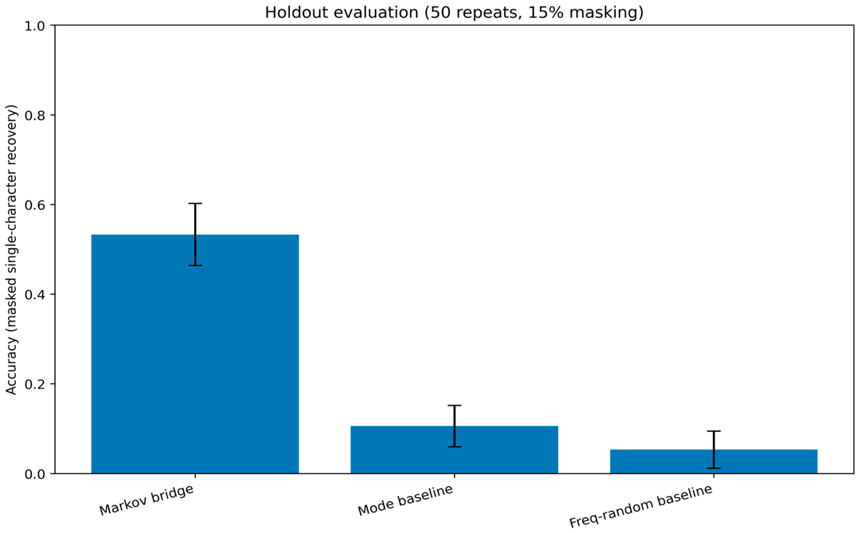
In order to determine whether the model is modelling non-trivial structure, as opposed to simply being able to recreate world frequency, we conduct a masked character recovery test on known text. An eligible test position is a test position that has seen neighbours to the left and right, which are also seen, giving 231 eligible test positions in the dataset. Each time, we repeat 50 times, we randomise 15 per cent of eligible positions on each line and apply a non-adjacency constraint, such that evaluation targets are isolated single-character gaps. This results in 35 masked targets per repeat (1750 total targets).
To predict the missing ID x of each masked target, the model maximises the local bridging score of P(x|left)P(right|x), defined using the learned bigram probabilities. In 50 repeats, the average highest−1 recovery accuracy is 0.533 (SD 0.069). Two baselines made of modes are far less successful: a mode baseline, predicting the most frequent ID in the world, always returns 0.106 (SD 0.046), and a frequency-matched random baseline returns 0.053 (SD 0.042). These findings (mean ± SD) are summarised in Figure 5.
In this analysis, the main task that the method is developed to solve is purposely the prediction of a single missing symbol based on its immediate neighbour context only. In such a restricted way, the evaluation isolates and validates the main role of the model in a clean way.
Though the framework may be extended in future work to evaluate a wider range of reconstructions over time, higher-order dependencies, and wider linguistic plausibility, a more evidentially thorough validation like this is highly significant. This large performance difference between our Markov model and the experimented baselines gives clear and positive answers to two important claims: first, that the position-preserving encoding effectively represents a retrievable local structure in the transcription, and second, that the success of the algorithm is due to actual pattern recognition, rather than simply exploiting the worldly frequencies of symbols.
This targeted outcome provides a solid, decipherable foundation of the core skill of the method and substantiates its usefulness in the local and evidence-based micro-restoration it was constructed to carry out.

4.4. Confidence Estimation and Calibration

To use the system professionally, there should be uncertainty communication. We then calculate a per-position confidence score as a result of the posterior distribution on candidate IDs based on the same local model. Given one missing position with these symbols, left and right, the un-normalised posterior of x is proportional to P(x|left)P(right|x). In the case of multi-position bounded gaps (length 2–5), the exact posterior marginals are calculated with a forward–backward pass having fixed boundaries.
The confidence values are assigned to each position, which is summarised as log(p1/p2), where p1 and p2 are the most likely and the second most likely posterior probability of that position. This measure can be interpreted: values that are close to zero suggest ambiguity (top candidates are almost equal), whereas larger values suggest that there is more preference towards the best candidate. The average of this log ratio over the positions in the gap is called gap-level mean confidence (reported in Figure 8); it is not the same value as the entire-sequence relative probabilities reported in Figure 9 (see Section 4.5).
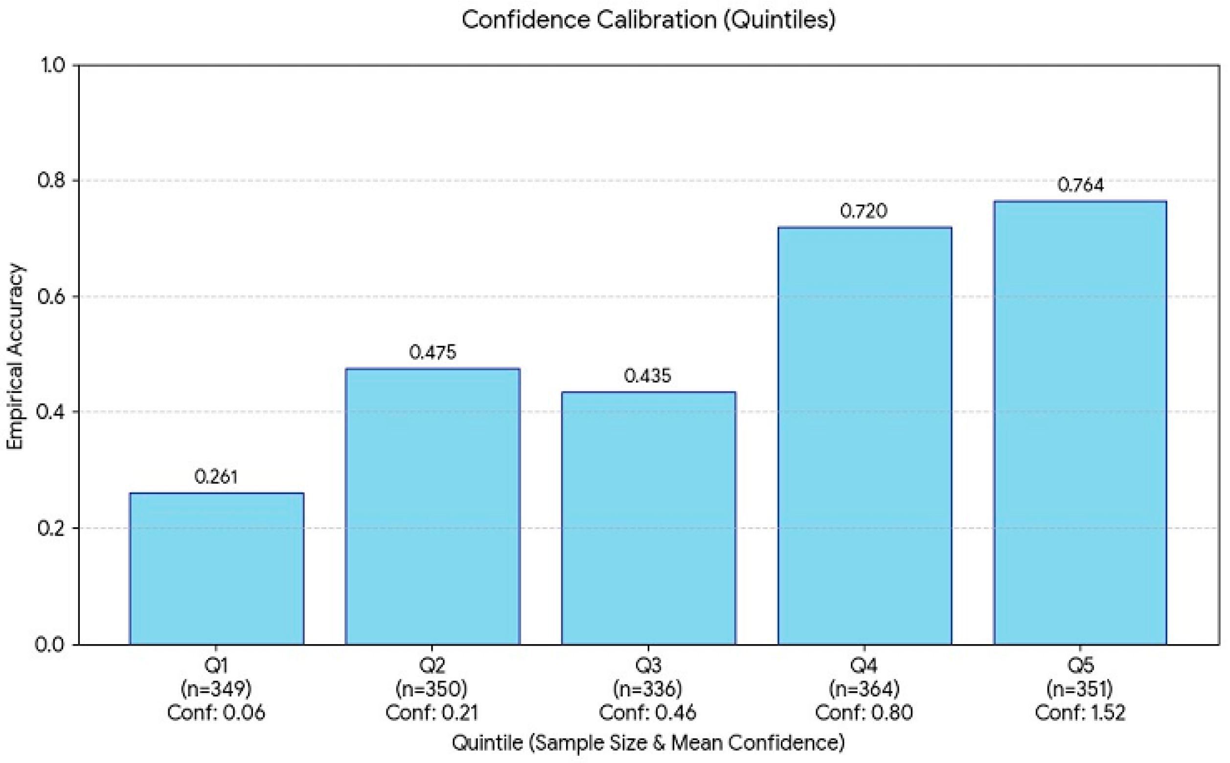
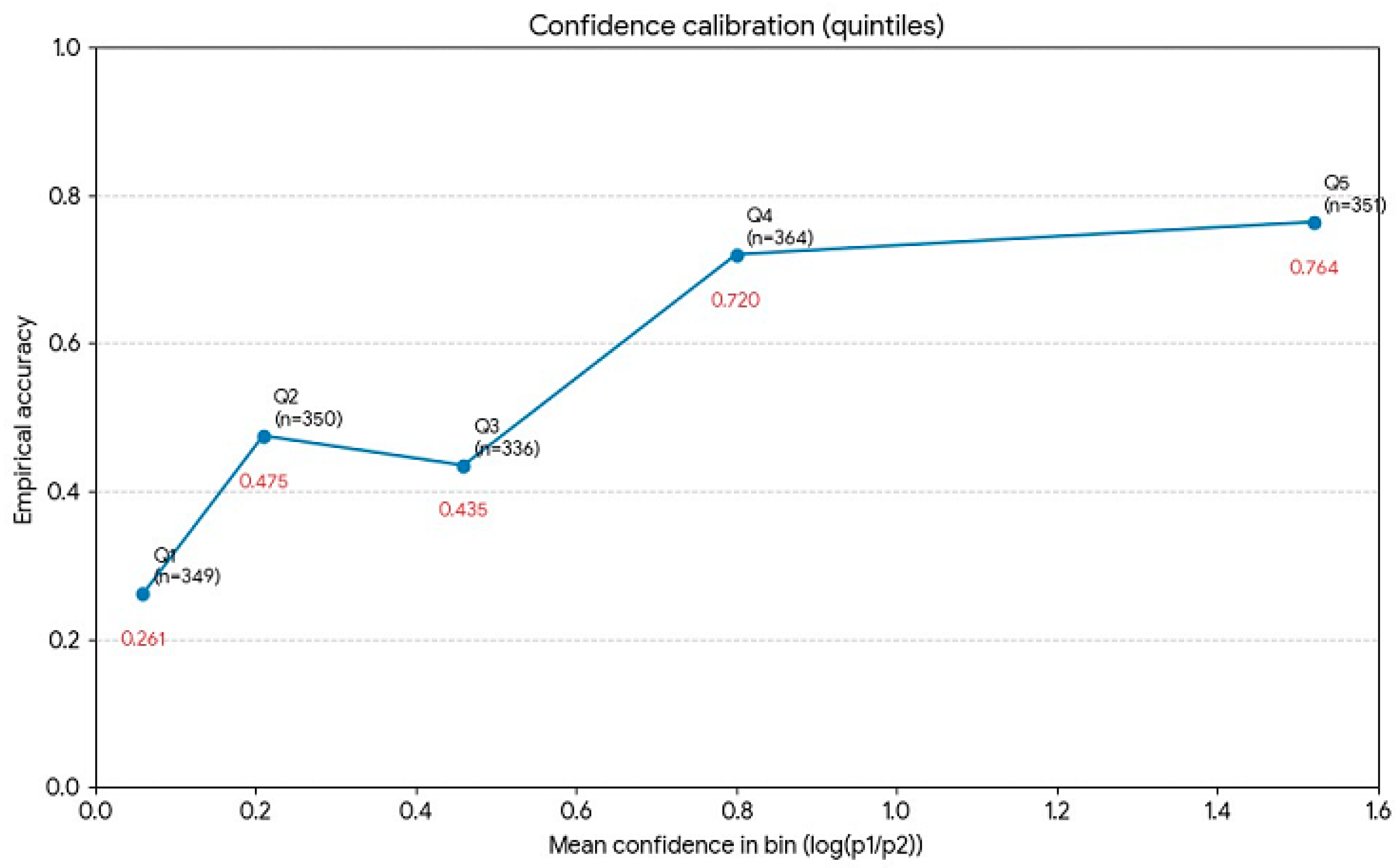
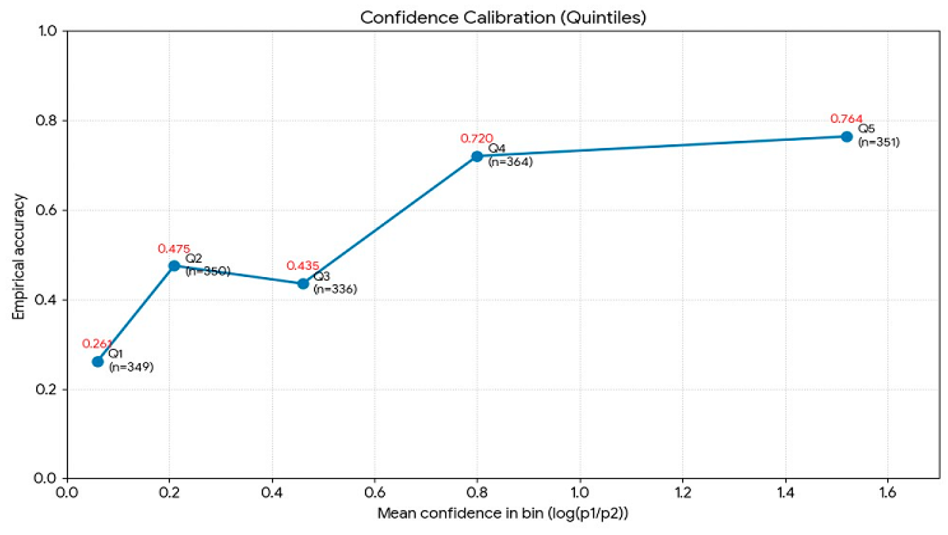
The masked character test gives a direct calibration test: in case confidence is useful, then high-confidence predictions should be correct more frequently. In all 1750 masked predictions, we take confidence in quintiles and derive empirical accuracy in each bin. Confidence increases accuracy dramatically, from 0.261 in the lowest quintile to 0.764 in the highest quintile; the mid-range bins have 0.474, 0.435, and 0.720, respectively. This relationship is visualised in Figure 6. The high distinction between low and high confidence justifies the use of confidence as an expert-facing indicator of which suggestions are most reliable.
In order to determine the reliability of internal scoring of the model, we determine the calibration of projected confidence and empirical accuracy. We use the log ratio of the first and second most likely predictions, log(p1/p2), as a confidence measure and divide the test set into five equal quintiles (Q1–Q5).
This model shows a positive correlation between internal certainty and actual performance, where the correlation is strong, as depicted in Figure 6. The empirical accuracy usually has an upward trend, with 0.261 as the lowest confidence 1st percentile (Q1) and increasing to 0.764 as the highest 1st percentile (Q5). Although the data displays a slight non-monotonic variation at Q3 (0.435), the general direction is the same: the greater the log confidence scores, the greater the predictive success, which provides a good proxy. Assigning a clear numerical value to every data point in Figure 6 guarantees complete transparency between the trends that the model illustrates and the metrics that were re-reported, which allows it to be concluded that the confidence of the model is well-calibrated to tackle decision-making tasks.

4.5. Real-World Applications of Concrete Restoration and Sets of Candidates

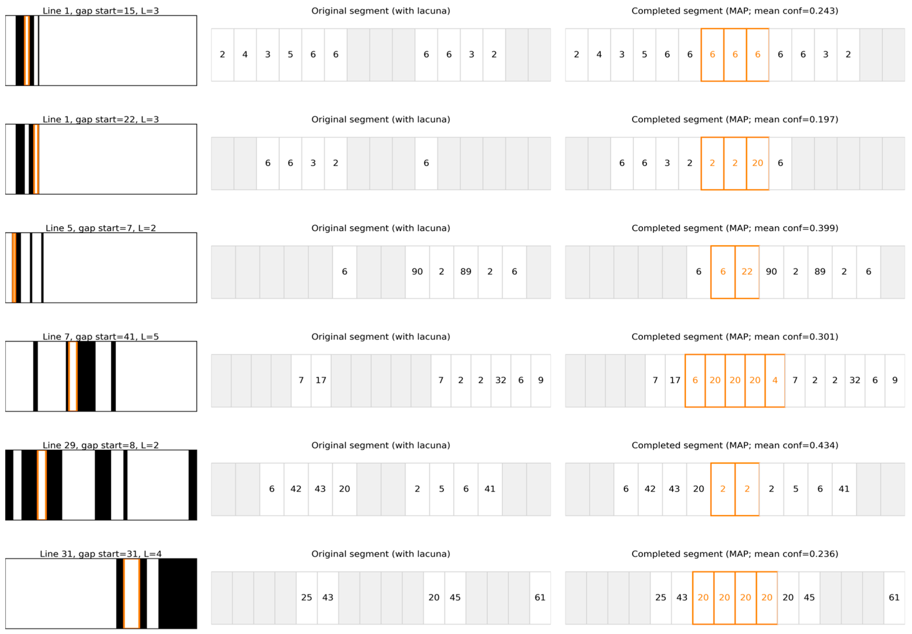
One of the issues raised in the review was that, in earlier drafts, there is no indication of what the algorithm would actually recommend to epigraphists. We have thus given two complementary perspectives of the output of restoration. Figure 9 and Figure 10 present six sample-bounded gap repairs (K = 5) as before/after panels and the known top five candidate sequences with their normalised relative probabilities in the top-five set, respectively.
The panels in Figure 7 are made by directly building them off the gap report that the pipeline provided. In each of the cases, the left panel displays the entire line in the form of a position map: where cells are observed, they are black; where they are missing, they are light grey, and the gap is indicated by a black line. The retracted distance between the line by the middle panel is maintained. The finished line is displayed in the right panel and the IDs added are highlighted. The confidence of each completion is the average log(p1/p2) given over the gap positions.
The six examples in Figure 8 are the following (all values are directly obtained at α = 0.5 and K = 5). The dimensions of the position map inscription in Figure 4 are 32 units wide and 219 units long. Two distinct three-slot bounded gaps can be found in Line 1: the completion at gap start = 15 ((6, 6, 6)) has mean completion = 0.243, and the completion at gap start = 22 ((2, 2, 20)) has mean completion = 0.197. There is a two-slot filled gap in Line 5 at gap start = 7 (between 6 and 90) filled in as 6, 22 (mean confidence = 0.399). At gap start = 41 (between 17 and 7) in Line 7, there is a gap with five slots to fill, and this gap is filled with the values 6, 20, 20, 20, 4 (mean confidence = 0.301). In Line 29, there is a two-slot bounded gap with gap start = 8 (between 20 and 2) filled in as 2, 2 (mean confidence = 0.434). Lastly, Line 31 has a four-slot bounded gap at gap start = 31 (between 43 and 20) filled as 20, 20, 20, 20 (mean confidence = 0.236).
For every example, the full line position map (left), zoomed original segment (centre), and zoomed completed segment (right) are shown. The highlighted IDs are those that have been inserted; the mean calculated confidence is the mean of log(p1/p2) across the gap.
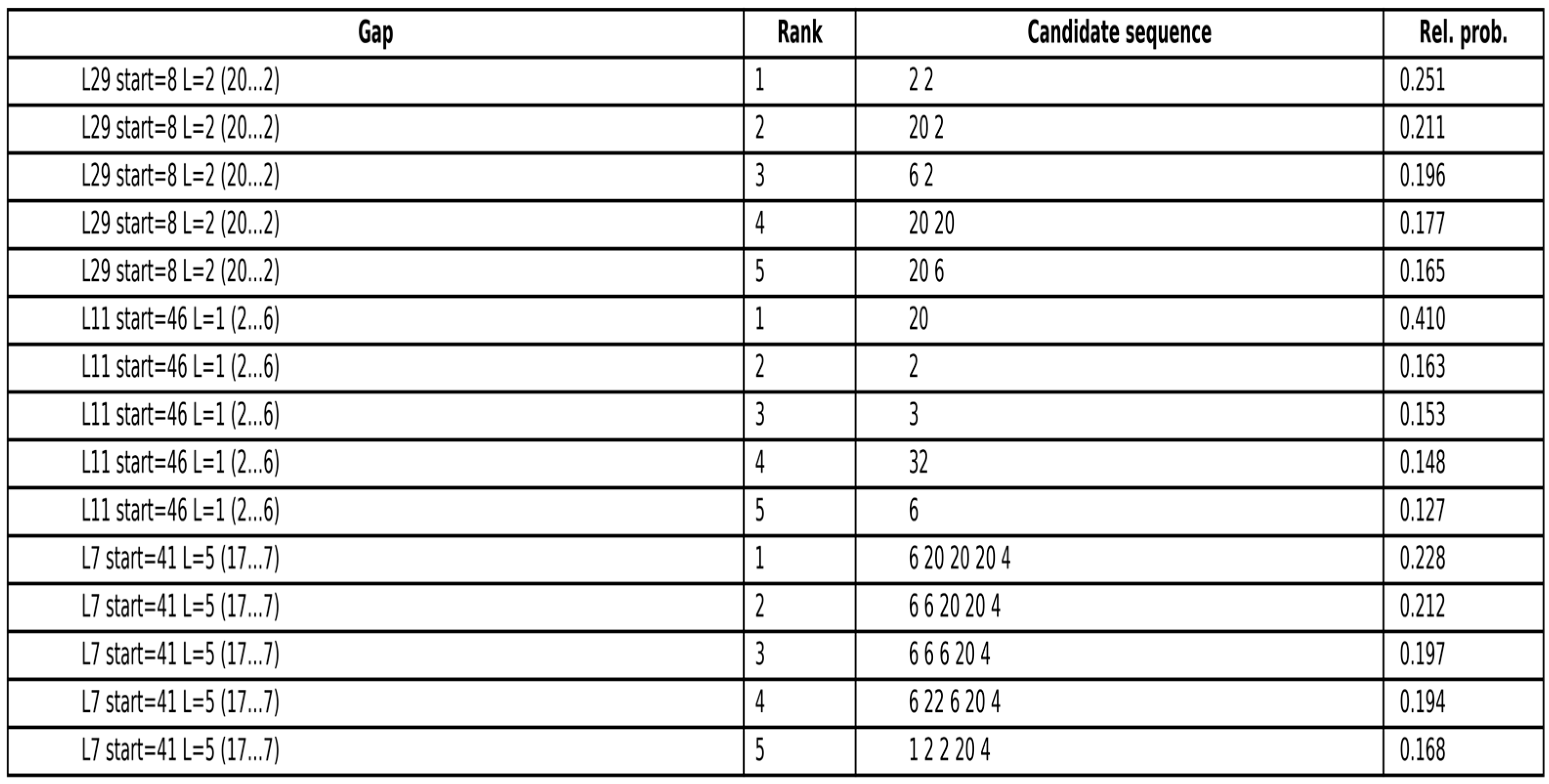
These panels are supplemented by Figure 9, as it exposes candidate diversity. With a given bounded gap, it is possible that there are several possible sequences. The table indicates the five most likely sequences of the same local model and indicates their relative probabilities as part of that set of 5 (the sum of the values represents 1). These are not per-position confidence scores but are the aggregate sequence probabilities, as shown in Figure 7.
In the case of the Line 29 gap (gap start = 8, gap length = 2, gap boundaries = 20, 2), the best candidate sequence (candidate sequence with highest relative probability) is 2, 2, and the relative probability of this sequence is 0.251. Nevertheless, there are still some competitive alternatives: 20, 2 (0.211), 6, 2 (0.196), 20, 20 (0.177), 20, 6 (0.165). This is among the cases when the tool should be used in the form of a hypothesis enumerator: it proposes the best completion, but also points at close options that a specialist can take into consideration as compared with palaeographic or linguistic evidence.
In the case of the single-slot gap (gap start = 46, bounds 2 and 6) in Line 11, the candidate with the highest probability is ID 20 with a relative probability of 0.410. The next candidates are 2 (0.163), 3 (0.153), 32 (0.148), and 6 (0.127). In cases of single slots, the differentiation between top candidates tends to correspond to greater mean confidence, since only one vacancy will be resolved.
In the case of the Line 7 five-slot gap (gap start = 41, end 17 and 7), the optimal sequence is 6, 20, 20, 20, 4 with a relative probability of 0.228. Other candidates indicate that the uncertainty spreads across the internal positions: 6, 6, 20, 20, 4 (0.212), 6, 6, 6, 20, 4 (0.197), 6, 22, 6, 20, 4 (0.194), and 1, 2, 2, 20, 4 (0.168). This set of rankings makes the ambiguity clear and avoids giving the false impression of a unique completion.
Probabilities are standardised against the top-five set; the fraction of certainty of the model over these gaps is summarised in the mean confidence scores in Section 4.5.

4.6. Sensitivity, Mislabel Invariance, and Missingness Assumptions

The maximum eligible gap length K and the strength of smoothing α are controlled by two modelling options: K and α. Where there are different K values, the number of repaired sites is altered, but the long lacunae remain un-mended. In this dataset, K = 1 occupied 3 gaps (3 positions), K = 3 occupied 12 gaps (27 positions), and K = 5 occupied 17 gaps (50 positions). Making the footprint of the restoration auditable under the K reporting helps avoid accidentally attempting to repair parts of the structure in a hypothetical global rebuilding.
Smoothing α affects predictive sharpness in sparse transition graphs. Using the same masked-character protocol as Section 4.3, α = 0.1 yields mean accuracy 0.590, α = 0.5 yields 0.533, α = 1.0 yields 0.472, and α = 2.0 yields 0.441. Stronger smoothing reduces contrast between plausible and implausible transitions and lowers accuracy in this dataset. Figure 4, Figure 5, Figure 6, Figure 7, Figure 8, Figure 9 and Figure 10 report results for α = 0.5, so that completion outputs and validation statistics are generated from the same fixed-parameter setting.
The Markov process is categorical by nature, with the aim of maintaining the integrity of the model. It does not consider integer numbers (ordinal) or numeric values, but merely makes use of equality of labels and observed transition frequencies among states. This plan cushions against enforcing spurious mathematical designs and determines a semantically neutral depiction of the coded epigraphic data. One of these direct directives is a relabelling invariance test: take any random permutation of the ID/integer mapping, run the pipeline, and decode the predictions back, and the resulting completed sequences should be the same. Independent completions with two distinct random re-labellings were found to give the same bounded gap completions on an inverse mapping showing that numeric neighbourhood effects are not seen as dominating predictions, but as dominated by the transition structure.
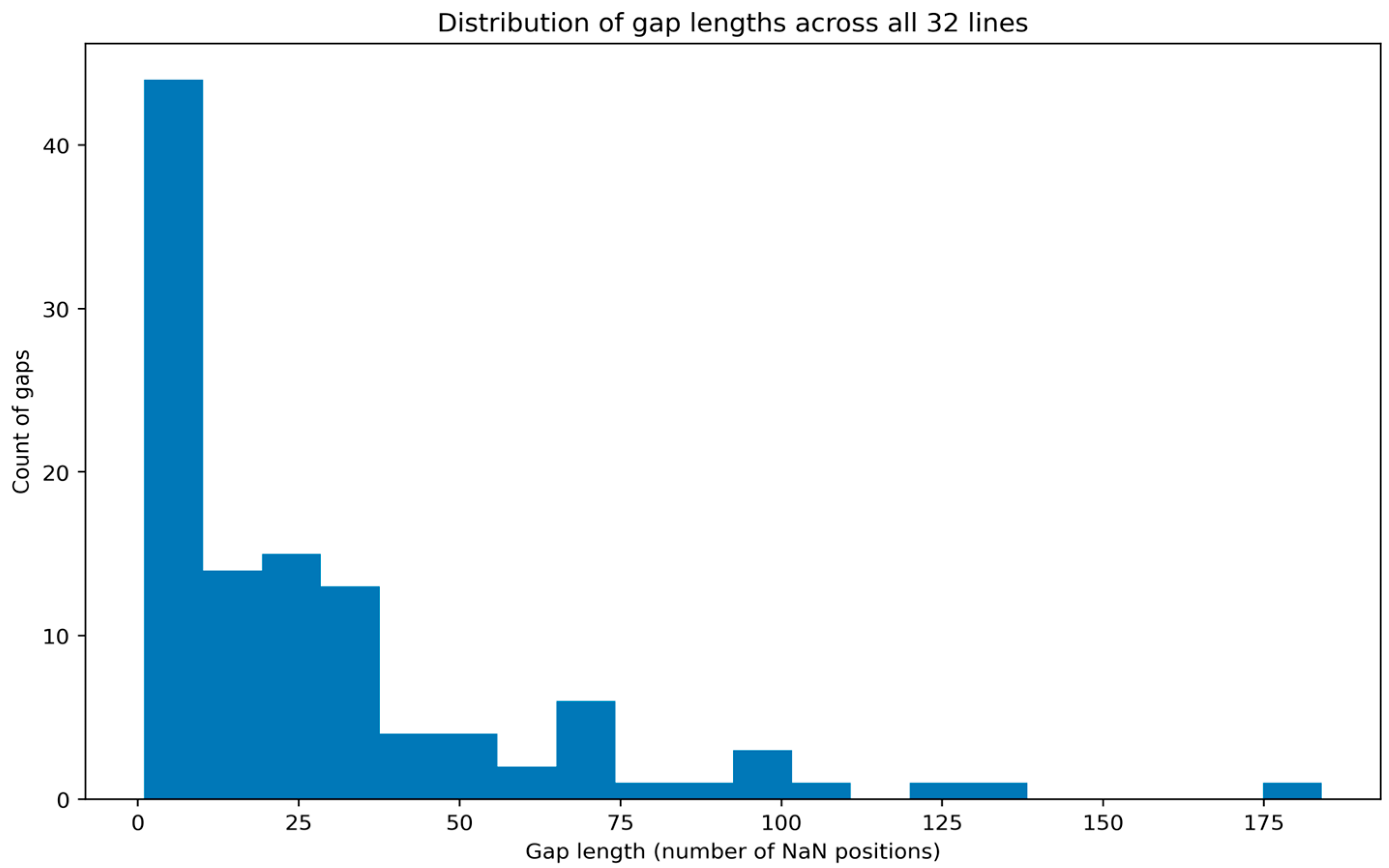
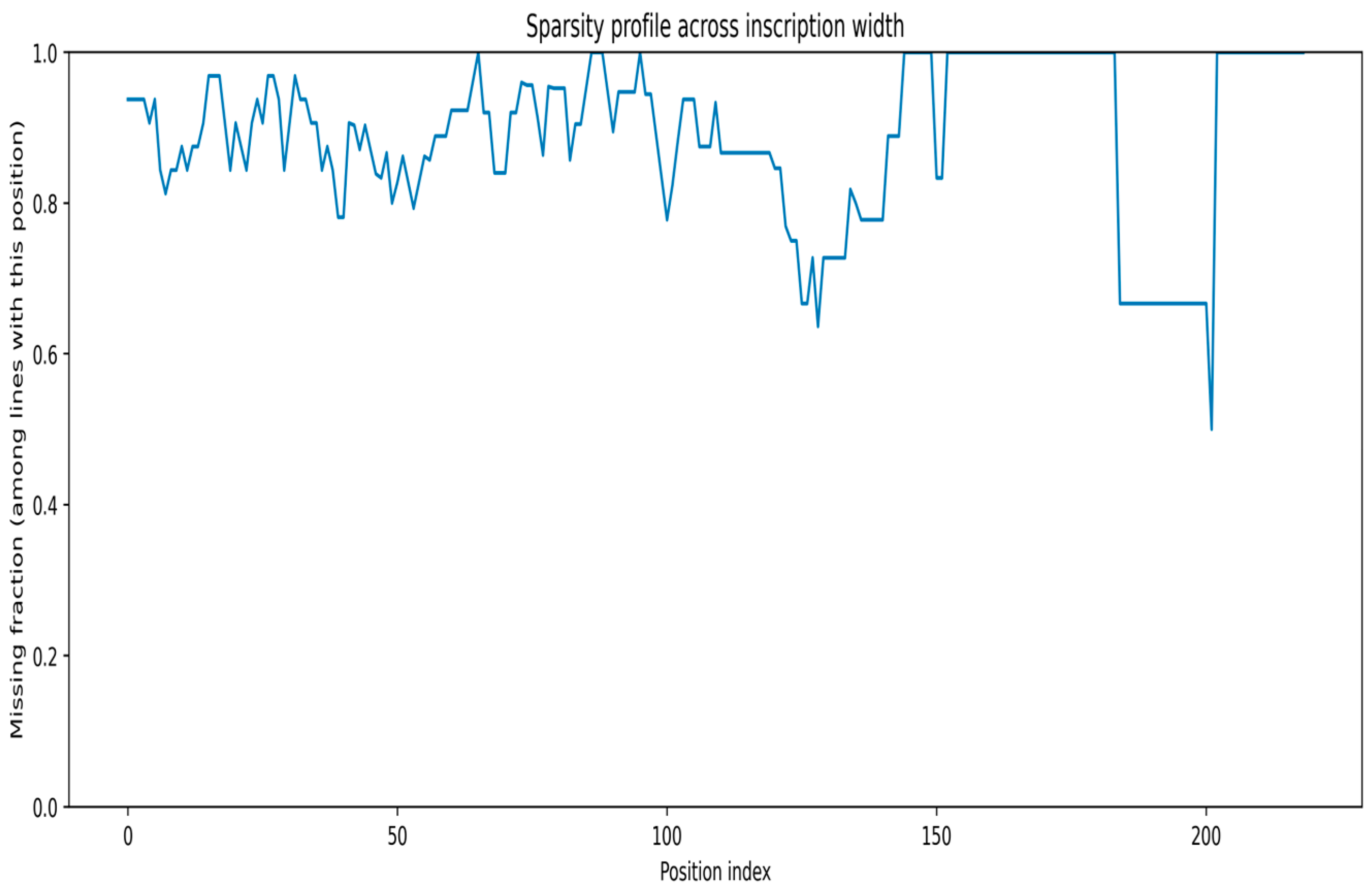
Lastly, the epigraphic content that has been lost is seldom missing at random. The patterns of systematic lacunae due to the breakage patterns and edge loss may be observed in the heavy-tailed gap length distribution (Figure 11) and the fact that the missingness depends heavily on position indices (Figure 12). In order to preserve model integrity, we repeat the statement that the Markov process is a categorical process: it is not a numeric or ordinal procedure that uses integer numbers, but merely takes equality of labels and observed frequencies of transitions between states. In such a manner, arbitrary mathematical structures are avoided, and the coded epigraphic information is maintained in a semantically neutral representation. The pipeline improves the quality of results by choosing to predict only in scenarios with immediate evidential support. It guarantees the reliability and traceability of its reconstructions by including only short and well-grounded spans, avoiding speculation in larger gaps where context is unavailable. The confidence in generating a verifiable local hypothesis space provides a solid foundation for further work. Any extensions, such as incorporating explicit damage models or image-based evidence, would adhere to this principled structure, ensuring that future developments remain grounded in demonstrably local evidence.
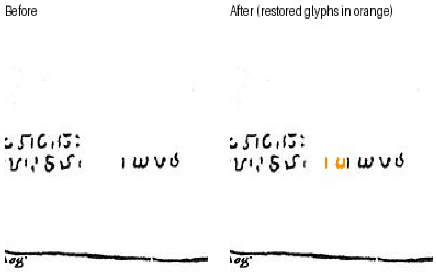
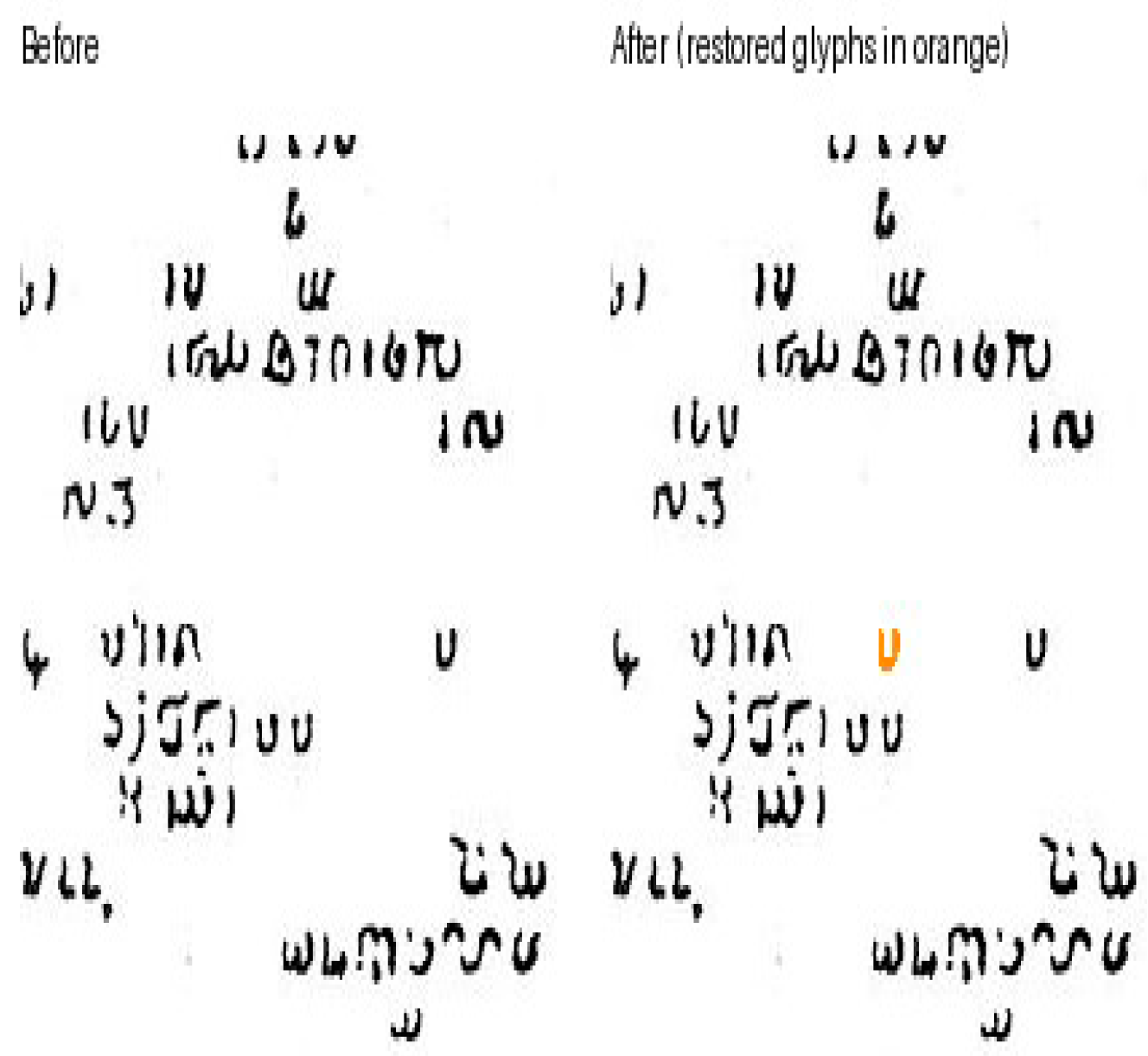
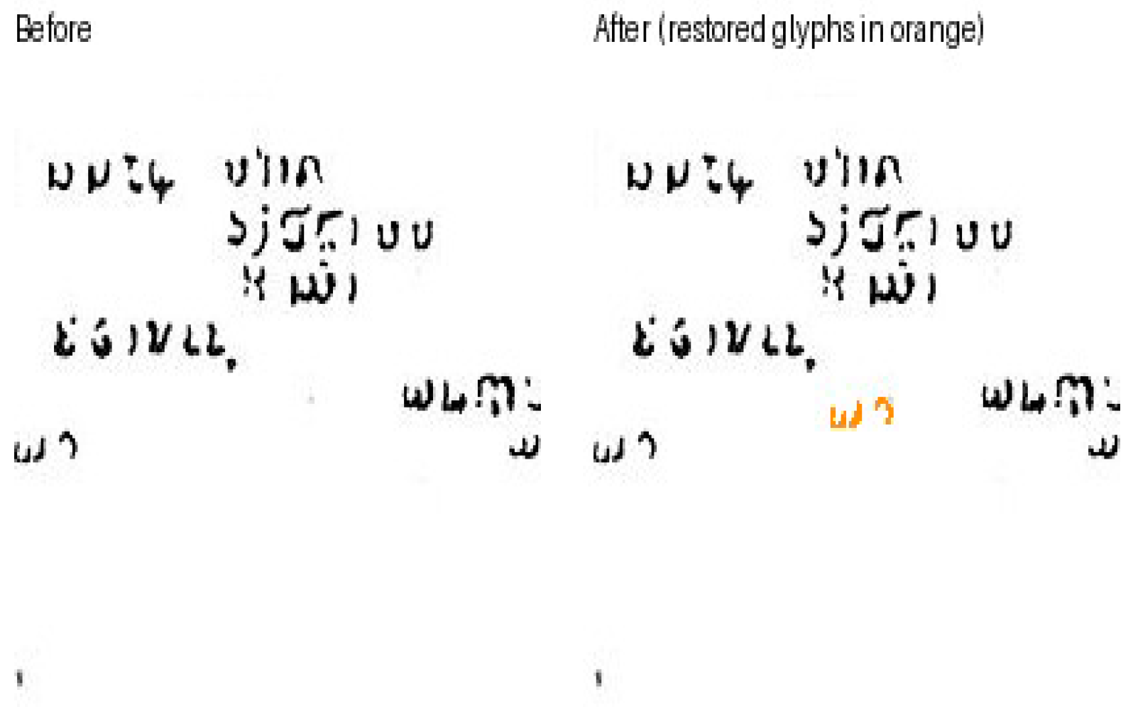
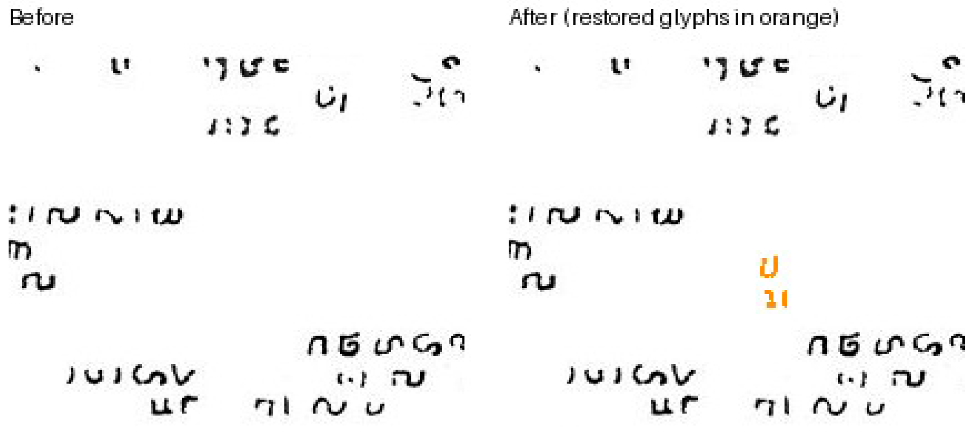
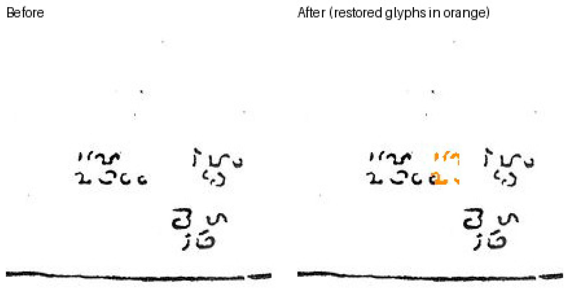
In order to turn the ID-level restorations into the readings available to epigraphists, we restore visualisations of some of those bounded gap completions by once again rendering them as glyph-level restoration overlays (Figure 13, Figure 14, Figure 15, Figure 16 and Figure 17). This reconstruction model is defined on the position-preserving encoded matrix definition (IDs are categorical states; missing slots are NaN) on its own. However, as a numeric ID cannot be viewed by a human reader, filled outputs are reconstructed into glyph examples to be observed. Every image in Figure 13, Figure 14, Figure 15, Figure 16 and Figure 17 is presented in the form of a ‘before/after’ panel: the former is represented by the reference to the original inscribed piece of the text with a visible lacuna (damage or blank space) and the latter superimposes the suggested restored glyph/s of the prototype at its former location/s. More importantly, these overlays provide an explicit view of the hypothesis generated by the very same conservative rule applied in the rest of the paper (internal gaps only, with a maximum gap length of K = 5). With this glyph-level display, specialists are able to identify the palaeographic viability of the offered completion in its immediate context, without affecting the workflow, and can re-create such a graphical request in the form of the underlying ID predictions and gap reports.
Left: original cut piece of the inscription with a missing area that is localised. Right: the same segment with the model-imputed glyph exemplar(s) in orange at an internal gap (K = 5) according to the position-preserving representation that is encoded.
The algorithm offers a localised completion (bounded NaN run) which is short and adds a visualisation to the completion by overlaying the reconstructed glyph exemplar(s) in orange at the slot(s) which are missing. Lacunae that are long are left unfilled.
Left: the original crop; right: the restored glyph insertion (in orange) by the same Markov-bridge completion rule applied to obtain the quantitative results (bounded gaps only; K 5), thus allowing the plausibility of the plausible ones to be checked by the experts themselves.
Conservative bounded-gap repair is marked as an overlay in the form of an orange line within the inscription area, showing how numbered predictive enumeration overrides are translated into something understandable to a human reader as an enumerative restoration theory, leaving observed strokes around the repair untouched.
The reinstated glyph exemplar(s) (orange) are only implanted at the demarcated point of the gap, and the rest of the fragmentary area is maintained. This illustrates the workflow as an expert-facing hypothesis generator and not a global reconstructive system.

5. Conclusions

The current paper describes a unique and replicable system of interpreting micro-restoration of very tiny inscriptions as a structured variable of absent data, but this is chiefly valuable for epigraphists. This underlying novelty is a position-preserving encoding scheme: each instance of character space is converted into an explicit absent position, thereby ensuring that the transcription leaves the geometry of the original line intact and allows one to ask purposeful and location-dependent restoration queries, which are directly related to the artefact.
In our categorical bigram bridging model, applied to this representation, we offer a deliberately conservative construction mechanism of bridging. It merely utilises observed adjacencies amongst coded IDs and does not attempt to traverse gaps that are not evidentially supported. The K = 5 constraint and the bounded-gap rule are principled methodological safeguards that ensure that the workflow is veridical with respect to the claims it can make with the data it has. In practice, this provides a set of local conjectures, which are well-grounded but do not constitute a complete, systematic reconstruction.
Quantitative assessment supports this locally based approach. The mean top-one accuracy of the model in masked character recovery is 0.533 across 50 repetitions, which is far superior to both mode and frequency-matched random baselines. It demonstrates that the transcription does not exclusively encode global symbol frequency as its meaningful local structure. Particularly in the analysis of expert adoption, the model confidence scores are highly functional: as the model assigns higher confidence to predictions, the empirical accuracy increases, which implies that confidence is a tool that can be effectively used for triage. The system does not suggest a single opaque restoration; it provides a list of ranked options for each gap, allowing epigraphists to take into consideration any external information, including parallel texts and grammatical and palaeographic data, to make their decision.
The same principled design decisions, which also determine the scope of the system, facilitate transparency. The sparsity and non-random missingness of the data, as well as the first-order transition model, are evidence of the fact that the system is not in a position to encode higher-order linguistic regularities, and this points to the actuality of the constraints: this system is an efficient hypothesis generator, but not an autonomous decipherment engine. Finally, performance is grounded on open routine encodings, and this points out the importance of transcription practices.
The structure allows numerous extensions to future operation without compromising its internal verifiability and scientific intent. To begin with, the training corpus should be extended to similar inscriptions, which would enhance transition statistics without breaching the bounded-gap layouts. Moreover, the higher-order or variable-order types of categorical models can be added to be able to learn longer-scale patterns of the locality without being able to trade off interpretability, especially when associated with transparent ablation studies and uncertain reporting. Additionally, evidence in terms of images, like stroke similarity or damage models, may be integrated, and that would perhaps mend the symbolic explanation with the physical properties of artefacts and turn the existing overlay demonstrations into multi-modal validation frameworks in their entirety.
Altogether, this paper provides a generalizable and practical template for computational epigraphy in high-missingness scenarios: preserve positional integrity, operate with conservative models, communicate uncertainty, and provide restorations as ranked, testable hypotheses that can augment—but not replace—professional epigraphical judgement.


Supplementary Materials

The following supporting information can be downloaded at https://drive.google.com/file/d/1C5DQ0IHcYGvLU2BempzZ-UIGIQKqK3ek/view?usp=drive_link, Python Code (accessed on 10 December 2025).

Author Contributions

Conceptualization, T.Z. and F.P.C.; methodology, T.Z. and F.P.C.; software, M.T.Z.; validation, T.Z. and F.P.C.; formal analysis, T.Z.; investigation, T.Z. and F.P.C.; resources, T.Z. and F.P.C.; supervision, F.P.C.; data curation, T.Z. and M.T.Z.; image curation, T.Z.; writing—original draft preparation, T.Z.; writing—review and editing, T.Z. and F.P.C.; fieldwork and archival research: F.P.C. All authors have read and agreed to the published version of the manuscript.

Funding

This research received no external funding.

Institutional Review Board Statement

Not applicable.

Informed Consent Statement

Not applicable.

Data Availability Statement

The original contributions presented in this study are included in the article/Supplementary Materials. Further inquiries can be directed to the corresponding authors.

Acknowledgments

We would like to acknowledge Muhammad Faisal Rasheed for his valuable contributions and support during this research. All individuals named in this section have reviewed and consented to this acknowledgment.
Conflicts of Interest

The authors declare no conflicts of interest.

References

  1. Yap, K.C.; Jiao, T.; Perono Cacciafoco, F. The Singapore Stone: Documenting the origins, destruction, journey and legacy of an undeciphered stone monolith. Histories 2023, 3, 271–287. [Google Scholar] [CrossRef]
  2. Heng, D. Diversity at a port city in Southeast Asia: The case of Singapore in the fourteenth century. Cult. Connect. 2017, 2, 47–56. Available online: https://www.researchgate.net/publication/318215710_Diversity_at_a_Port_City_in_Southeast_Asia_The_Case_of_Singapore_in_the_Fourteenth_Century (accessed on 9 December 2025).
  3. Colless, B.E. The ancient history of Singapore. J. Southeast Asian Hist. 1969, 10, 1–11. [Google Scholar] [CrossRef]
  4. Littleredlore. Singapore Legends: Badang and the Singapore Stone. 2025. Available online: https://littleredlore.wordpress.com/2025/05/14/singapore-legends-badang-and-the-singapore-stone/ (accessed on 9 December 2025).
  5. Leyden, J. Malay Annals; Longman, Hurst, Rees, Orme, and Brown: London, UK, 1821. [Google Scholar]
  6. Miksic, J.N. Archaeological Research on the ‘Forbidden Hill’ of Singapore: Excavations at Fort Canning, 1984; Singapore National Museum: Singapore, 1985. [Google Scholar]
  7. National Heritage Board. Our Top Twelve Artefacts. Available online: https://www.nhb.gov.sg/ (accessed on 14 November 2025).
  8. National Museum of Singapore. Singapore Stone. Available online: https://www.nlb.gov.sg/main/article-detail?cmsuuid=0a757a02-5f6b-483a-8a32-97a09953da63 (accessed on 14 November 2025).
  9. bin Abdul Kadir, A. The Hikayat Abdullah: The Autobiography of Abdullah bin Abdul Kadir (1797–1854); Hill, A.H., Translator; Oxford University Press: Oxford, UK, 1969. [Google Scholar]
  10. Bland, W. Inscription on the jetty at Singapore. J. Asiat. Soc. Bengal 1837, 6, 680–682. [Google Scholar]
  11. Begbie, P.J. The Malayan Peninsula; Vepery Mission Press: Chennai, India, 1834. [Google Scholar]
  12. de Casparis, J.G. Indonesian Palaeography: A History of Writing in Indonesia from the Beginnings to c. A.D. 1500; Brill: Leiden, The Netherlands, 1975. [Google Scholar]
  13. Lee, I.-S.; Perono Cacciafoco, F. Unravelling the mystery of the Singapore Stone: A comparative analysis with the Calcutta Stone and the possible Kawi connection. Histories 2023, 3, 261–270. [Google Scholar] [CrossRef]
  14. Tee, E.-Y. In the shadow of the Rosetta Stone: The Singapore Stone, repatriation and decolonisation. AGON 2021, 11, 29–41. Available online: https://portale.unime.it/agon/files/2021/08/2906.pdf (accessed on 9 December 2025).
  15. Prinsep, J. Inscription on the jetty at Singapur. J. Asiat. Soc. Bengal 1837, 6, 680–681. [Google Scholar]
  16. Low, J. An account of several inscriptions found in Province Wellesley, on the Peninsula of Malacca. J. Asiat. Soc. Bengal 1848, xvii, 62–66. [Google Scholar] [CrossRef]
  17. Wikipedia. Singapore Stone. 2025. Available online: https://en.wikipedia.org/wiki/Singapore_Stone (accessed on 14 November 2025).
  18. Laidlay, J.W. Note on the inscriptions from Singapore and Province Wellesley. J. Asiat. Soc. Bengal 1848, xvii, 66–72. [Google Scholar]
  19. EpiDoc. EpiDoc Guidelines (TEI/EpiDoc for Ancient Documents). Available online: https://epidoc.stoa.org/ (accessed on 10 January 2026).
  20. Rubin, D.B. Inference and missing data. Biometrika 1976, 63, 581–592. [Google Scholar] [CrossRef]
  21. White, I.R.; Royston, P.; Wood, A.M. Multiple imputation using chained equations: Issues and guidance for practice. Stat. Med. 2011, 30, 377–399. [Google Scholar] [CrossRef] [PubMed]
  22. Van Buuren, S. Flexible Imputation of Missing Data, 2nd ed.; Chapman and Hall/CRC: Boca Raton, FL, USA, 2018. [Google Scholar]
  23. Rabiner, L.R. A tutorial on hidden Markov models and selected applications in speech recognition. Proc. IEEE 1989, 77, 257–286. [Google Scholar] [CrossRef]
  24. Viterbi, A.J. Error bounds for convolutional codes and an asymptotically optimum decoding algorithm. IEEE Trans. Inf. Theory 1967, 13, 260–269. [Google Scholar] [CrossRef]
  25. Griffiths, A. The corpus of inscriptions in the Old Malay language. In Writing for Eternity: A Survey of Epigraphy in Southeast Asia; Perret, D., Ed.; École Française d’Extrême-Orient: Paris, France, 2018; Volume 30, pp. 275–283. Available online: https://hal.science/hal-01920769 (accessed on 9 December 2025).
  26. Yeoh, B.S.A. Street-naming and nation-building: Toponymic inscriptions of nationhood in Singapore. Area 1996, 28, 298–307. [Google Scholar]
  27. Chua, B.H. Culture, Multiracialism, and National Identity in Singapore. In Trajectories, 1st ed.; Routledge: Oxfordshire, UK, 1998; pp. 18–35. Available online: https://www.taylorfrancis.com/chapters/edit/10.4324/9780203976586-11/culture-multiracialism-national-identity-singapore-chua-beng-huat (accessed on 9 December 2025).
  28. Mak, L.F. Rigidity of System Boundary Among Major Chinese Dialect Groups in Nineteenth-Century Singapore: A Study of Inscription Data. Mod. Asian Stud. 1980, 14, 465–488. [Google Scholar] [CrossRef]
  29. Gonzaga, F. Monsoon Marketplace: Inscriptions and Trajectories of Consumer Capitalism and Urban Modernity in Singapore and Manila; University of California: Berkeley, CA, USA, 2014; Available online: https://escholarship.org/uc/item/6tm6c0mx (accessed on 9 December 2025).
  30. Yap, M.T.; Koh, G.; Soon, D. (Eds.) Migration and Integration in Singapore: Policies and Practice; Routledge: Oxfordshire, UK, 2014. [Google Scholar] [CrossRef]
Figure 1. A localization map of the original site of the Singapore Stone at Rocky Point.
Information 17 00170 g001
Figure 3. Different types of Kawi were reproduced digitally.
Information 17 00170 g003
Figure 4. The character position map of the inscription.
Information 17 00170 g004
Figure 5. Masked single-character target holdout test (50 repeats, 15% masking per line; mean ± SD).
Information 17 00170 g005
Figure 6. Calibration of confidence: empirical accuracy at confidence quintile on log(p1/p2) (3 same).
Information 17 00170 g006
Figure 7. Mean log-confidence vs. data quintiles empirical accuracy.
Information 17 00170 g007
Figure 8. Distribution of prediction accuracy vs. confidence bin.
Information 17 00170 g008
Figure 9. Bounded gap examples of representative restoration (K 5).
Information 17 00170 g009
Figure 10. Constructed variations in sample bounded gaps.
Information 17 00170 g010
Figure 11. Gap length distribution along the 32 encoded lines.
Information 17 00170 g011
Figure 12. Profile of sparsity across inscription width (lost fraction of lines which hold each position).
Information 17 00170 g012
Figure 13. Example of before/after glyph restoration.
Information 17 00170 g013
Figure 14. Glyph restoration.
Information 17 00170 g014
Figure 15. Restored glyphs, on the right.
Information 17 00170 g015
Figure 16. Image 4: restored glyphs.
Information 17 00170 g016
Figure 17. Restored glyphs.
Information 17 00170 g017
Disclaimer/Publisher’s Note: The statements, opinions and data contained in all publications are solely those of the individual author(s) and contributor(s) and not of MDPI and/or the editor(s). MDPI and/or the editor(s) disclaim responsibility for any injury to people or property resulting from any ideas, methods, instructions or products referred to in the content.