Long-Term Air Quality Data Filling Based on Contrastive Learning

Abstract

Continuous missing data is a prevalent challenge in long-term air quality monitoring, undermining the reliability of public health protection and sustainable urban development. In this paper, we propose ConFill, a novel contrastive learning-based framework for reconstructing continuous missing data in air quality time series. By leveraging temporal continuity as a supervisory signal, our method constructs positive sample pairs from adjacent subsequences and negative pairs from distant and shuffled segments. Through contrastive learning, the model learns robust representations that preserve intrinsic temporal dynamics, and enable accurate imputation of continuous missing segments. A novel data augmentation strategy is proposed, to integrate noise injection, subsequence masking, and time warping to enhance the diversity and representativeness of training samples. Extensive experiments are conducted on a large scale real-world dataset comprising multi-pollutant observations from 209 monitoring stations across China over a three-year period. Results show that ConFill outperforms baseline imputation methods under various missing scenarios, especially in reconstructing long consecutive gaps. Ablation studies confirm the effectiveness of both the contrastive learning module and the proposed augmentation technique.

1. Introduction

Air quality plays a critical role in human health, ecosystems, and global climate change. With the rapid urbanization and industrialization, air pollution has become a widespread environmental challenge worldwide. To effectively monitor and assess air quality, modern air quality monitoring systems rely on dense networks of sensors and monitoring stations. However, due to equipment failures, data transmission failures, or extreme weather conditions, monitoring data often contains missing values. Such a data gaps can hinder accurate assessments and early warnings of air quality. Therefore, developing effective approaches to fill missing air quality data has become an urgent research priority.

Beyond conventional automatic monitoring networks, an increasing number of applied air quality studies rely on in situ and proxy-based monitoring approaches to characterize urban pollution under realistic environmental conditions. These approaches include indirect or surrogate measurements that provide valuable environmental insights but are frequently affected by practical operational constraints, such as episodic pollution events, sensor saturation, equipment maintenance, and the deployment of low-cost sensing devices [1,2]. Consequently, missing data in air quality monitoring are not solely the result of random sensor failures but often arise from systematic and scenario-dependent factors inherent to real-world monitoring practices. Such missingness commonly manifests as continuous data gaps within otherwise regularly sampled time series, posing substantial challenges for accurate data reconstruction and downstream environmental analysis.

Traditional statistical imputation methods typically include mean imputation, interpolation, and regression analysis [3]. These methods are simple to implement and computationally efficient, providing reasonable estimates when data missingness is minimal. Mean imputation replaces missing values with the mean of the entire or local dataset, making it suitable for scenarios where missingness is relatively random and the proportion of missing data is small. Another commonly used method is interpolation, which includes linear interpolation and spline interpolation [4]. These methods estimate missing data based on the relationships between known data points. Their advantages include intuitive operation, low computational overhead, and the absence of complex models or algorithms. However, when dealing with large-scale or complex-structured data, their accuracy and robustness often deteriorate, leading to systematic biases.

Regression analysis is another commonly used traditional approach. It predicts missing values by modeling statistical relationships between the missing entries and other variables [5]. Although such imputation methods can be effective in certain cases, they depend heavily on predefined mathematical or statistical assumptions. This reliance limits their applicability when the dataset becomes complex [6]. In general, traditional statistical methods perform well on small datasets with low missing ratios. However, their performance often deteriorates when handling large-scale, high-dimensional, and complex air quality datasets, leading to less accurate imputation results [7,8].

With the advancement of machine learning techniques, learning-based imputation methods have gained increasing attention. Compared with traditional statistical approaches, machine learning models generally demonstrate stronger generalization capability and robustness when modeling nonlinear relationships in large datasets [9]. Commonly used methods include decision trees, random forests, support vector machines, and k-nearest neighbors algorithms [10,11,12]. These methods leverage observed data to construct predictive models for estimating missing values. Nevertheless, their performance remains sensitive to feature selection, data quality, and computational scalability. When applied to large-scale air quality datasets with heterogeneous and non-random missing patterns, conventional machine learning methods often incur high computational costs and exhibit limited effectiveness in reconstructing long continuous missing segments [13].

With the rapid advancement of data-driven technologies, deep learning has emerged as a powerful framework for processing and imputing air quality data. Deep learning models, particularly neural networks, can automatically extract complex representations from large datasets and recover missing data through multi-layer nonlinear mappings. Compared to traditional machine learning methods, deep learning does not require explicit feature engineering, as it can automatically learn the latent patterns from raw data [14]. Commonly used deep learning architectures include convolutional neural networks (CNNs), recurrent neural networks (RNNs), and generative adversarial networks (GANs) [15,16,17]. Convolutional neural networks (CNNs) have also been widely adopted for air quality data imputation due to their strong capability in capturing local patterns and short-range dependencies in structured data [18]. In contrast, RNN-based models, especially long short-term memory (LSTM) networks, are more suitable to handle missing data with temporal dependencies. They can effectively utilize contextual information in time series to achieve more precise imputation of missing temporal data [19]. MLP is a feedforward neural network composed of multiple layers of neurons (including an input layer, several hidden layers, and an output layer). Unlike CNNs and RNNs, MLP connects neurons in each layer to those in the preceding layer through fully connected layers. It is suitable for processing simpler data patterns and can learn latent patterns in data through multi-layer nonlinear mapping [20].

In recent years, the successful application of Transformer architectures in natural language processing has garnered widespread attention, and their powerful modeling capabilities have begun to be introduced into tasks such as air quality prediction and data imputation. Transformer models leverage self-attention mechanisms to capture global contextual relationships, making them particularly effective at handling complex data correlations. Compared to RNNs and CNNs, Transformers overcome the time complexity bottlenecks inherent in traditional recurrent neural networks, thereby enhancing computational efficiency [21,22]. As research deepens, models improved upon the Transformer have demonstrated outstanding performance across multiple tasks and domains. The Informer model addresses long-term sequence data modeling challenges, proving particularly suitable for time series forecasting [23]. The Conformer model combines CNNs and Transformers to enhance local feature processing capabilities [24]. FedFormer is a federated learning model based on Transformers [25]. The Reformer model reduces computational complexity in Transformer architectures [26]. Autoformer effectively improves model performance when handling seasonal variations and long-term dependencies in time-series data [27].

The advantage of deep learning methods lies in their ability to model complex nonlinear relationship in data structures and scale to large-scale air quality monitoring networks. However, these methods also present significant challenges, including high computational costs, substantial data requirements for training, and potential overfitting issues [28]. Moreover, their limited interpretability remains a major concern, often requiring integration with other analytical or statistical models to better understand and validate the decision-making process.

Motivated by these challenges, this study proposes a novel contrastive self-supervised learning framework specifically designed for continuous missing segment imputation in air quality time series. The proposed approach jointly exploits time-domain and frequency-domain representations to capture both temporal dynamics and spectral characteristics of air quality data. By introducing contrastive learning as an auxiliary self-supervised objective, the framework learns robust latent representations from incomplete observations, enabling effective reconstruction of long missing segments without relying on complete supervision. Extensive experiments conducted on datasets collected from multiple monitoring stations demonstrate that the proposed framework consistently outperforms state-of-the-art baseline methods in terms of accuracy and robustness. The main contributions of this study are summarized as follows:

• A self-supervised learning mechanism is designed to infer the latent representations of missing data and align them with the embeddings of observed data. This alignment enables the model to learn intrinsic correlations between input and output features without the need for complete supervision.
• The model adopts a contrastive learning objective in which the missing segments of the same sample are treated as positive pairs, while those from other samples in the batch are treated as negative pairs. Through innovative data augmentation strategies, the diversity of positive samples is enriched, allowing the model to learn more discriminative features by maximizing similarity within positives and minimizing similarity with negatives.
• An integrated imputation framework is developed to capture complex temporal dependencies in air quality time series, achieving improved robustness and generalization performance for long-term and continuous air quality data reconstruction.

2. Methods

2.1. Problem Description

The Air Quality Index (AQI) is a comprehensive indicator that reflects the overall level of air pollution. It is typically calculated based on the concentrations of several major pollutants, including PM_2.5, PM₁₀, SO₂, NO₂, O₃, and CO. Different AQI ranges correspond to varying degrees of health impact, where higher AQI values indicate more severe pollution and greater risks to human health [29].

In this study, we consider an air quality monitoring network comprising S stations, each reporting observations at fixed hourly intervals. Due to sensor malfunctions, data transmission failures, routine maintenance, and adverse environmental conditions, air quality records collected in real-world monitoring systems often contain missing observations. Robust reconstruction methods are therefore required to recover incomplete AQI time series under such non-ideal monitoring conditions.

Let $X\in {\mathbb{R}}^{S\times T\times F}$ denote the complete spatio-temporal dataset, where T represents the number of time steps and F denotes the number of observed features. In addition to AQI, we consider six meteorological variables related to air quality, including rainfall, humidity, air pressure, temperature, wind speed, and wind direction. The AQI value recorded at station i and time step j is denoted by $A_{i,j}\in [0, 500]$, while $X_{i,j,f}$ represents the value of the f-th meteorological feature.

Specifically, for a consecutive missing segment of length $l_t$ at a given station, two neighboring observation windows are extracted. These include $X_a\in {\mathbb{R}}^{N\times l_a}$, corresponding to the $l_a$ time steps immediately preceding the missing segment, and $X_b\in {\mathbb{R}}^{N\times l_b}$, corresponding to the $l_b$ time steps immediately following it. By jointly modeling the temporal dynamics and feature correlations within these adjacent segments, the proposed method aims to reconstruct the missing AQI sequence of length $l_t$ in an accurate and consistent manner.

2.2. Data Preprocessing

2.2.1. Data Preparation

Contrastive learning is a self-supervised method that constructs positive and negative sample pairs to drive the model to learn the similarities and differences in the data. This method is particularly suitable for scenarios without explicit labels. It can learn the underlying data structure by designing positive and negative sample pairs, making it applicable to the problem of filling in long-term time-series data [30]. Contrastive learning maximizes the similarity between positive sample pairs and minimizes the differences between negative sample pairs, enabling it to automatically learn the temporal dependencies and long-term relationships within sequence data [31]. This allows for a better understanding of the complex connections between different time points in the sequence. Its goal is to learn effective feature representations to capture both short-term and long-term dependencies in time-series data. This, in turn, helps the model fill in more accurate and reasonable values when data is missing.

During training, continuous missing segments of varying lengths are explicitly constructed and treated as reconstruction targets, ensuring that the organization of the training data is directly aligned with the objective of long-term consecutive missing data imputation. Contrastive learning is applied to the observed contextual subsequences adjacent to the missing segments, rather than to the missing values themselves. Importantly, by constructing positive and negative samples that preserve realistic temporal continuity and contextual dependencies, the encoder is encouraged to learn representations that are robust to continuous data gaps arising from non-ideal monitoring conditions, thereby improving the reliability of the reconstructed AQI sequences for practical environmental applications.

Given a batch of n time-series segments $S_1,S_2,\dots ,S_n$, each segment corresponds to a contiguous temporal window extracted from the original dataset. For each segment $S_i$, a fixed-length subsequence $L_i$ is selected as the anchor representation. A positive sample $P_i$ is then generated by applying a combination of time-domain and frequency-domain augmentation operators to $L_i$. Since both $L_i$ and $P_i$ originate from the same raw segment, they share consistent temporal semantics and form a valid positive pair under the contrastive objective. All other anchors $L_j\mid j\ne i$ within the same batch are treated as negative samples, as they are derived from different temporal contexts and encode distinct local dynamics.

This batch-wise construction is compatible with the InfoNCE loss, where each anchor participates in one positive pair and $n-1$ negative pairs. By maximizing similarity between positive pairs while minimizing similarity to negatives, the encoder is encouraged to learn discriminative and temporally aware representations that preserve meaningful temporal structures. Repeated optimization across diverse temporal windows enables the model to construct a smooth latent space that is well suited for downstream reconstruction tasks.

Figure 1 illustrates the positive and negative sample construction strategy, where green arrows indicate positive associations and red arrows denote negative relationships within each batch.

Next, data augmentation is applied to the positive samples to increase the diversity of the training data, thereby improving the model’s generalization ability and robustness to noise. During the validation stage, a threshold-based detection method is used to filter out samples exhibiting abnormal fluctuations or unstable patterns, retaining only those that meet the predefined stability criteria for model evaluation. The threshold is determined according to preset rules to ensure that the samples used for validation maintain sufficient quality and consistency, enabling a more accurate assessment of the model’s predictive performance.

Through these processing steps, the code converts the original multidimensional time-series data into structured samples suitable for model training and validation. The resulting sample sets include enhanced and processed positive and negative samples. They also contain non-mutated data that are used for evaluation during the validation stage. Together, these samples allow the model to learn patterns in time-series data more effectively and support reliable predictions in real-world scenarios.

2.2.2. Consecutive Missing Segment Construction

To explicitly align the training process with the task of long-term missing data reconstruction, continuous missing segments are deliberately simulated during training. For each station-level time series, a consecutive temporal interval of length $l_t$ is randomly selected and masked, with $l_t$ sampled from a predefined range to represent different durations of sensor outages or data transmission failures.

The masked segment is removed from the input sequence and treated as the reconstruction target, while the observed segments immediately before and after the missing segment are retained as contextual inputs. By repeatedly exposing the model to samples containing explicitly constructed consecutive missing segments, the training process enforces a direct correspondence between the learning objective and realistic missing data patterns. These samples are further incorporated into the contrastive learning framework, where segments with similar temporal contexts form positive pairs and unrelated segments serve as negative pairs, enhancing representation discriminability while preserving the intrinsic characteristics of continuous missing patterns.

2.2.3. Data Augmentation

We propose a joint time-domain and frequency-domain data augmentation method that enhances the robustness and generalization ability of models by performing multi-level augmentation processing on time-series data, making it suitable for tasks that rely on time series features. The specific method combines time-domain augmentation techniques and frequency-domain augmentation techniques to generate diverse training samples.

Time-domain data augmentation primarily increases data diversity by simulating temporal changes, missing values, or shifts within time series. In this method, time-domain augmentation primarily includes two operations: time shifting and time step masking.

First, the input data is a long time series $x\left(t\right)$ in the time domain, where t is the length of the time series. The time shift operation shifts the time series by a random amount s (forward or backward):

$$x^{\prime }\left(t\right)=x(t+s)$$

After applying time-domain augmentation, the enhanced signal is transformed into the frequency domain using the Fourier transform. In the frequency domain, the amplitude is denoted as $A\left(f\right)=\left|X\right(f\left)\right|$, and the phase is represented by $\theta \left(f\right)=arg\left(X\right(f\left)\right)$. Enhancement operations in the frequency domain mainly include noise enhancement and frequency component rearrangement. In the frequency domain, we dynamically adjust the noise intensity based on the amplitude of each frequency component and add adaptive noise to different frequency components. The noise level is proportional to the amplitude of the frequency component:

$$N\left(f\right)=\eta ·\left({\displaystyle \frac{A\left(f\right)}{max\left(A\right(f\left)\right)}}\right)·\mathcal{N}(0, 1)$$

where $\eta$ is the noise intensity, $\mathcal{N}(0, 1)$ is the noise generated by the standard normal distribution, and the amplitude after noise enhancement is $A^{\prime }\left(f\right)=A\left(f\right)+N\left(f\right)$. This ensures that the enhanced data retains the main features of the original signal while introducing moderate changes to improve the model’s generalization ability.

Next, the amplitude of the frequency components is normalized, and the probability of rearrangement is adjusted according to the amplitude. Frequency components with smaller amplitudes are given a higher probability of random exchange. Calculate the adaptive rearrangement rate

$$P_{\mathrm{shuffle}}\left(f\right)=\lambda \left(1-{\displaystyle \frac{A^{\prime }\left(f\right)}{max\left(A^{\prime }\left(f\right)\right)}}\right)$$

where $\lambda$ is the parameter that controls the rearrangement ratio. Then, randomly select some frequency components and swap their positions:

$$A^{″}\left(f_1\right)=A^{\prime }\left(f_2\right), A^{″}\left(f_2\right)=A^{\prime }\left(f_1\right)$$

By performing this adaptive rearrangement of frequency components, data diversity can be effectively increased while preserving the signal’s primary characteristics. Finally, the processed signal is converted back to the time domain via an inverse Fourier transform (IFFT), with the real part taken as the enhanced time-series data. By jointly applying time-domain and frequency-domain augmentation, the proposed strategy enriches data diversity across both temporal and spectral dimensions. This joint enhancement improves the model’s robustness to temporal distortions and frequency variations, which is particularly beneficial for learning discriminative representations from complex time-series data [32].

2.3. Model Architecture

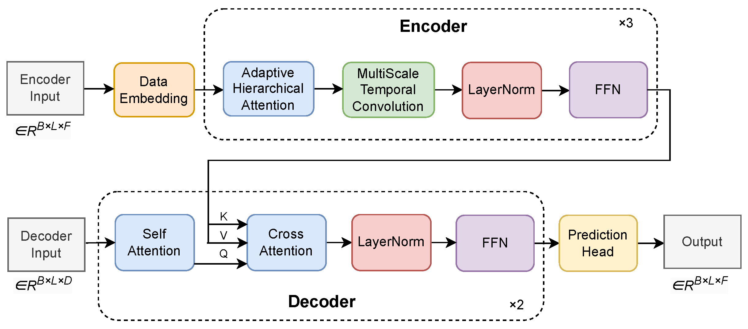
This paper proposes a sequence-to-sequence prediction model based on multi-scale convolutions and an adaptive hierarchical attention mechanism, aimed at addressing long-term sequence prediction tasks. The model integrates frequency-domain feature embedding, an adaptive attention mechanism, multi-scale convolution operations, and a transformer structure to enhance prediction accuracy by efficiently extracting diverse features from temporal data. By processing anchor, positive, and negative samples at the same time, the model captures both temporal and frequency-domain relationships among different sequences. This design enhances its robustness and generalization ability. Experiments further show that the model delivers strong prediction performance across multiple benchmark datasets.

The core of this model consists of the following main components: data embedding module, encoder module, decoder module, and prediction head module. The model utilizes an adaptive hierarchical attention (AHA) mechanism, multi-scale temporal convolution (MSTC) structure, and feedforward neural network (FFN) to process sequence data. Combined with frequency domain feature embedding, this further enhances the model’s ability to represent temporal data. The model structure is shown in Figure 2.

2.3.1. Data Embedding Module

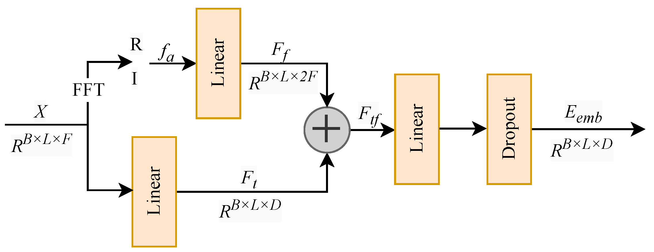
The data embedding module aims to project raw air quality time-series data into a unified high-dimensional representation space, providing informative inputs for subsequent encoder–decoder modeling. To jointly capture temporal dynamics and frequency-domain characteristics, both time-domain and frequency-domain representations are incorporated in the embedding process.

Given an input time series X, a fast Fourier transform (FFT) is first applied to convert the signal from the time domain into the frequency domain. The resulting complex-valued frequency representation consists of real and imaginary components, denoted as R and I, respectively. The corresponding frequency amplitude is computed as

$$fa=\sqrt{R^2+I^2}.$$

Next, the frequency domain feature $F_f$ is obtained through the linear projection and mapped to the model embedding representation dimension D. The formula for the linear transformation is as follows:

$$F_f=W^{\top }x+b,$$

where $W\in {\mathbb{R}}^{D\times C}$ is the learnable weight matrix, C denotes the input feature dimension, and $b\in {\mathbb{R}}^D$ is the bias term. This transformation aligns the frequency-domain features with the model embedding dimension D, facilitating subsequent joint modeling.

In parallel, the original time-domain input is also projected into the same embedding space via a linear transformation, yielding the time-domain feature representation $F_t$. The time-domain and frequency-domain embeddings are then concatenated as $[F_t,F_f]$ to form a joint time–frequency representation $F_{tf}$. To ensure dimensional consistency, the concatenated features are further passed through a feature projection layer, which maps $F_{tf}$ back to the embedding dimension D.

Dropout regularization is applied to the projected embeddings to mitigate overfitting. The final output of the data embedding module, denoted as $E_{emb}$, integrates complementary information from both temporal and frequency perspectives. This representation serves as the input to the encoder module, enabling subsequent attention mechanisms to effectively model temporal dependencies while preserving the periodic and spectral characteristics of the time series. The overall architecture of the data embedding module is illustrated in Figure 3.

2.3.2. Encoder

The encoder module is designed to effectively capture both global and local temporal dependencies in long time-series data, which is critical for improving representation learning and imputation accuracy. To this end, we propose an encoder architecture that integrates adaptive hierarchical attention with multi-scale temporal convolution.

The encoder is composed of multiple stacked encoding layers, each consisting of an adaptive hierarchical attention module and a multi-scale temporal convolution block.

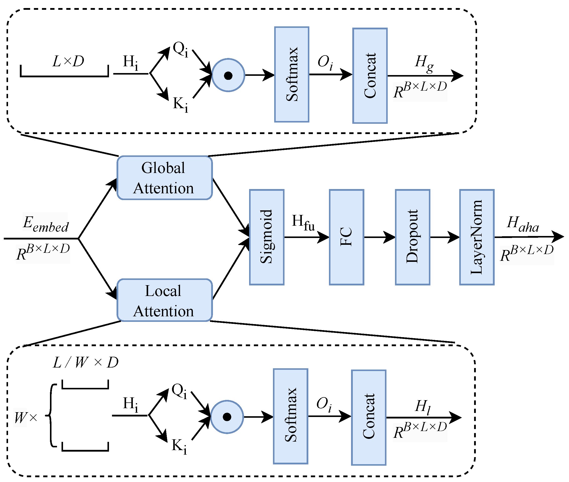
Adaptive hierarchical attention module: This module combines global attention and local attention to simultaneously model long-range dependencies and local contextual patterns. A gated fusion mechanism is introduced to dynamically balance the contributions of global and local attention based on input characteristics.

Given the embedded input features $E_{emb}$, the adaptive hierarchical attention mechanism jointly models global and local attention representations. For each attention head $H_i$, the global attention component captures long-term dependencies across the entire sequence, producing $H_g$, while the local attention component focuses on short-term dependencies within local windows, yielding $H_l$. The local attention operates within a predefined temporal window centered at each query position. The window size is fixed and shared across all samples during training, providing a stable inductive bias for modeling short-term temporal dependencies.

These two representations are adaptively fused through a learnable gating mechanism based on a Sigmoid activation function, allowing the model to dynamically adjust the importance of global and local information. The fused representation is then processed through a fully connected layer, followed by layer normalization and residual connections to enhance training stability and representation robustness. The overall workflow of the adaptive hierarchical attention module is illustrated in Figure 4.

The core objective of the adaptive hierarchical attention mechanism is to enable the model to fuse and weight-adjust information features from data embedding layer outputs across multiple levels by introducing global and local multi-layer multi-head attention operations. Ultimately, this yields feature representations $H_{aha}$ enhanced by multi-scale contextual information. This facilitates more effective capture of long-term and short-term dependencies as well as information from different hierarchical levels. Unlike traditional attention mechanisms that usually compute attention weights at a single level, the adaptive hierarchical attention mechanism adjusts weights across multiple levels. It integrates information progressively from local (short-term dependencies) to global (long-term dependencies) and flexibly balances their importance. Through this hierarchical structure, the model can also dynamically measure the correlations between different positions in the sequence, creating direct connections across layers. For example, lower-level features often capture fine-grained details, while higher-level features represent more abstract patterns. Hierarchical attention allows the model to decide which level is more important for the current task and to adjust the contribution of each layer accordingly.

The multi-head self-attention layer captures both global and local patterns by modeling global dependencies across the input sequence through its Query–Key–Value (Q-K-V). Given an input $E_{emb}\in {\mathbb{R}}^{B\times L\times D}$, the query (Q), key (K), and value (V) are derived after a permutation of its dimensions. Within this mechanism, the core operation involves computing the similarity between Q and K, which fundamentally extracts the global correlations across different time steps through a weighted aggregation. The multi-head mechanism computes the attention scores $Sco={\displaystyle \frac{Q{K}^{\top }}{\sqrt{d_k}}}$, $Sco\in {\mathbb{R}}^{B\times L\times D}$ for each head through projection calculations using h independent attention heads $H_i$ and their respective weight matrices $W_i^Q\in {\mathbb{R}}^{D\times d_k}, W_i^K\in {\mathbb{R}}^{D\times d_k}, W_i^V\in {\mathbb{R}}^{D\times d_v}$, $d_k=d_v=D/h$. These scores are normalized via Softmax for positions i and j, then weighted and summed to yield the feature for each head:

$${\mathrm{Score}}_{ij}={\displaystyle \frac{q_i·k_j}{\sqrt{d_k}}}={\displaystyle \frac{{\sum }_{m=1}^{d_k}{q}_{im}{k}_{jm}}{\sqrt{d_k}}}$$

$$A_{ij}=\mathrm{Softmax}\left(\mathrm{Scores}\right)={\displaystyle \frac{exp\left({\mathrm{Score}}_{ij}\right)}{{\sum }_{k=1}^{L}exp\left({\mathrm{Score}}_{ik}\right)}}$$

The output of a single attention head i is computed as $O_i={\sum }_{j=1}^L{A}_{ij}{V}_j$. The outputs from all heads are then concatenated into a composite representation $O_a=[O_1,O_2,\dots ,O_n]\in {\mathbb{R}}^{B\times L\times D}$. A subsequent linear projection is applied to $O_a$ to fuse the features from all heads, allowing them to interact and learn an optimal combination. This process yields a unified and enhanced sequence representation, denoted as the final results $h_g$ and $h_l$. The complete data flow is depicted in Figure 5.

Unlike conventional attention mechanisms that focus on a single temporal scope, the proposed adaptive hierarchical attention jointly models multiple temporal ranges within each encoding layer and adaptively fuses them through a gated mechanism. The formulas for GlobalAttention and LocalAttention are as follows:

$$GlobalAttention(Q,K,V)=\mathrm{softmax}\left({\displaystyle \frac{Q{K}^T}{\sqrt{d_k}}}\right)V$$

$$LocalAttention(Q,K,V)=\mathrm{softmax}\left({\displaystyle \frac{Q{K}^T}{\sqrt{d_k}}}\right)V$$

where Q, K, and V represent the query, key, and value matrices, respectively. After modeling global and local attention, the module concatenates the global attention output and local attention output through a gating mechanism. The Sigmoid activation function is used in the gating mechanism to fuse the outputs of global attention and local attention. The purpose is to obtain a weight (a value between 0 and 1) through learning to determine the contribution of global and local features. Through the gating mechanism, the weights of global and local attention are dynamically adjusted based on the context to fuse the two types of features:

$$H_{fu}=G·H_g+(1-G)·H_l$$

The gating weight $G\in [0, 1]$ is learned automatically from data and determines the relative contribution of global attention output $H_g$ and local attention output $H_l$, yielding the fused representation $H_{fu}$. The gate mechanism enables the model to dynamically adapt, balancing between global and local attention based on the characteristics of the input sequence, and adaptively selecting the optimal attention pattern under different contextual conditions. Finally, the output $H_{aha}$ of the data embedding layer is obtained through the fully connected layer and residual connections:

$$H_{aha}=\mathrm{LayerNorm}\left(Q+\mathrm{Dropout}\left(\mathrm{FC}\left(H_{fu}\right)\right)\right)$$

By integrating adaptive hierarchical attention with multi-scale temporal modeling, the encoder effectively captures temporal dependencies across different resolutions, improving robustness to noise, missing values, and long-term sequence variations.

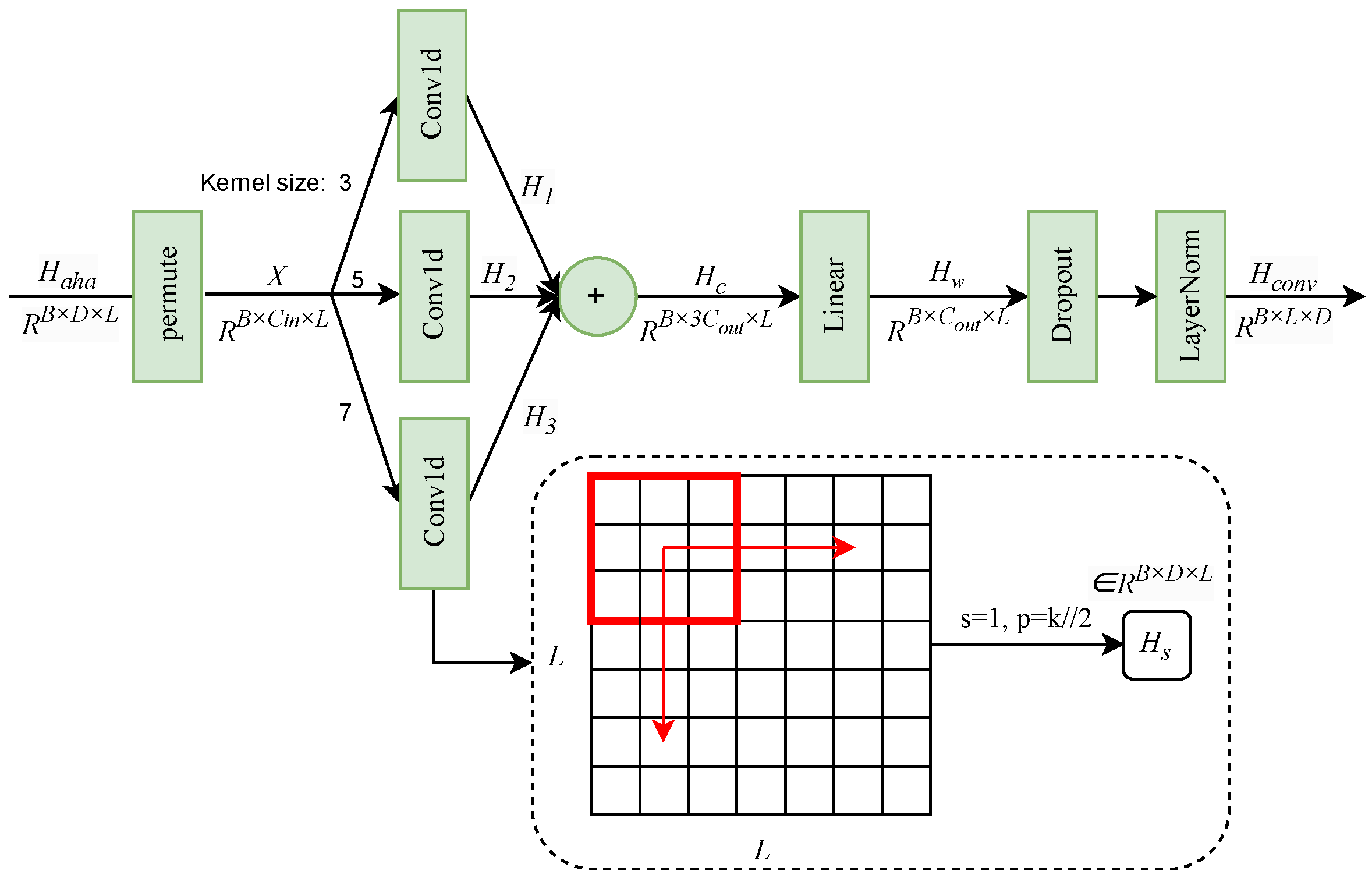
Multi-scale temporal convolution module: This module serves as a complementary local feature extractor to the attention mechanism, enabling the model to capture temporal patterns at multiple resolutions through convolution kernels of different sizes. While attention mechanisms are effective at modeling global dependencies, convolution operations focus on localized temporal structures, thereby enhancing the representation of short-range dependencies at different temporal scales. The overall workflow of the multi-scale temporal convolution module is illustrated in Figure 6.

We first transpose the output $h_{aha}$ of the adaptive hierarchical attention layer to form the input tensor $X\in {\mathbb{R}}^{B\times C_{in}\times L}$ for the multi-scale convolution module, where B denotes the batch size, $C_{in}=D$ is the embedding dimension, and L is the sequence length. The module employs multiple one-dimensional convolution kernels with different kernel sizes $K\in \{3, 5, 7\}$ to capture temporal patterns at different scales.

For each convolution scale s, the output feature map is computed as

$$H_s[b, c_{out}, t]=\sum _{c_{in}=0}^{C_{in}-1}\sum _{k=0}^{K_s-1}X[b, c_{in}, t+k]\times W_s[c_{out}, c_{in}, k]+b_s\left[c_{out}\right],$$

where $W_s\in {\mathbb{R}}^{C_{out}\times C_{in}\times K_s}$ and $b_s\in {\mathbb{R}}^{C_{out}}$ denote the convolution weights and bias at scale s, respectively.

The outputs from different scales are concatenated to form a multi-scale representation $H_c=[H_1,H_2,H_3]\in {\mathbb{R}}^{B\times \left(3C_{out}\right)\times L}$. A linear projection layer is then applied to fuse the multi-scale features:

$$H_w=W_{\mathrm{proj}}·H_c+b_{\mathrm{proj}},$$

resulting in a unified feature representation $H_w\in {\mathbb{R}}^{B\times L\times C_{out}}$.

Finally, residual connections, dropout, and layer normalization are applied to obtain the output representation $H_{conv}$. By integrating multi-scale convolution with attention-based representations, this module enhances the model’s robustness to noise, missing values, and temporal variations commonly observed in real-world sensor data, while effectively capturing both short-term fluctuations and long-term trends.

Feedforward neural network (FFN): The feedforward neural network is a standard yet essential component in the encoder and decoder layers, responsible for further transforming and refining the features extracted by the attention and convolution modules. It consists of two fully connected layers with a nonlinear activation function in between. The first linear layer projects the input features into a higher-dimensional intermediate space to enhance expressive capacity, followed by a ReLU activation to introduce nonlinearity and capture complex feature interactions. The second linear layer maps the intermediate representation back to the original feature dimension, ensuring compatibility with subsequent modules. Residual connections and normalization are incorporated to stabilize training and preserve feature consistency. In the proposed model, the FFN operates in a position-wise manner, enabling flexible nonlinear feature transformation for each time step, which is particularly beneficial for handling noisy and partially observed time series commonly encountered in real-world sensor data.

The feedforward network complements the attention and convolution mechanisms by enhancing local feature representations through nonlinear transformations, allowing the model to capture higher-order dependencies while maintaining computational efficiency.

Residual Connections and Layer Normalization: Residual connections and layer normalization are employed to improve training stability and facilitate deep feature learning. Residual connections enable direct information flow across layers by learning residual mappings, effectively mitigating gradient vanishing issues in deep architectures. Layer normalization standardizes intermediate feature distributions, accelerating convergence and improving robustness. These mechanisms are especially important in long time-series modeling scenarios with missing values or long consecutive data gaps, as they help maintain stable representations and reduce sensitivity to noise and distribution shifts.

Overall, the encoder integrates adaptive hierarchical attention, multi-scale temporal convolution, and position-wise feedforward transformation to jointly model global dependencies, local patterns, and nonlinear feature interactions within time-series data.

By combining attention-based long-range modeling with convolutional multi-scale feature extraction, the encoder is able to capture temporal dependencies across different resolutions while maintaining robustness to noise, missing values, and long-term temporal variations. This design is particularly well suited for real-world air quality monitoring data affected by sensor outages and complex environmental variations.

2.3.3. Decoder

The decoder integrates self-attention and cross-attention mechanisms to generate context-aware output representations. The self-attention layer models intra-sequence dependencies within the decoder input, ensuring temporal consistency and contextual coherence. The cross-attention layer explicitly incorporates information from the encoder output, enabling the decoder to leverage globally encoded temporal representations and improve reconstruction accuracy.

By querying the encoder representations, the cross-attention mechanism allows the decoder to selectively focus on relevant temporal contexts learned from the input sequence, which is particularly important for long-term time-series reconstruction tasks.

The cross-attention operation is formulated as

$$CrossAttention(Q,K,V)=\mathrm{Softmax}\left({\displaystyle \frac{Q{K}^T}{\sqrt{d_k}}}\right)V,$$

where Q, K, and V follow the standard attention convention but are derived from different sources: the query Q is obtained from the decoder states, while the key K and value V are projected from the encoder outputs.

During decoding, the input sequence is first processed by a self-attention layer to capture the internal temporal relationships. This is followed by a cross-attention layer that fuses encoder-derived contextual information with decoder features, enhancing the model’s ability to exploit long-range temporal dependencies. A feedforward neural network is then applied to perform nonlinear feature transformation and refinement.

This layered attention structure enables the decoder to effectively integrate local decoding dynamics with global temporal representations learned by the encoder, improving robustness to missing values and long-term temporal variations commonly observed in real-world sensor data.

Finally, the decoder output is projected to the model dimension D through a linear projection layer, yielding the final hidden representation $H_{dec}$, which encapsulates rich semantic and temporal information for subsequent missing data reconstruction.

2.3.4. Predictive Head

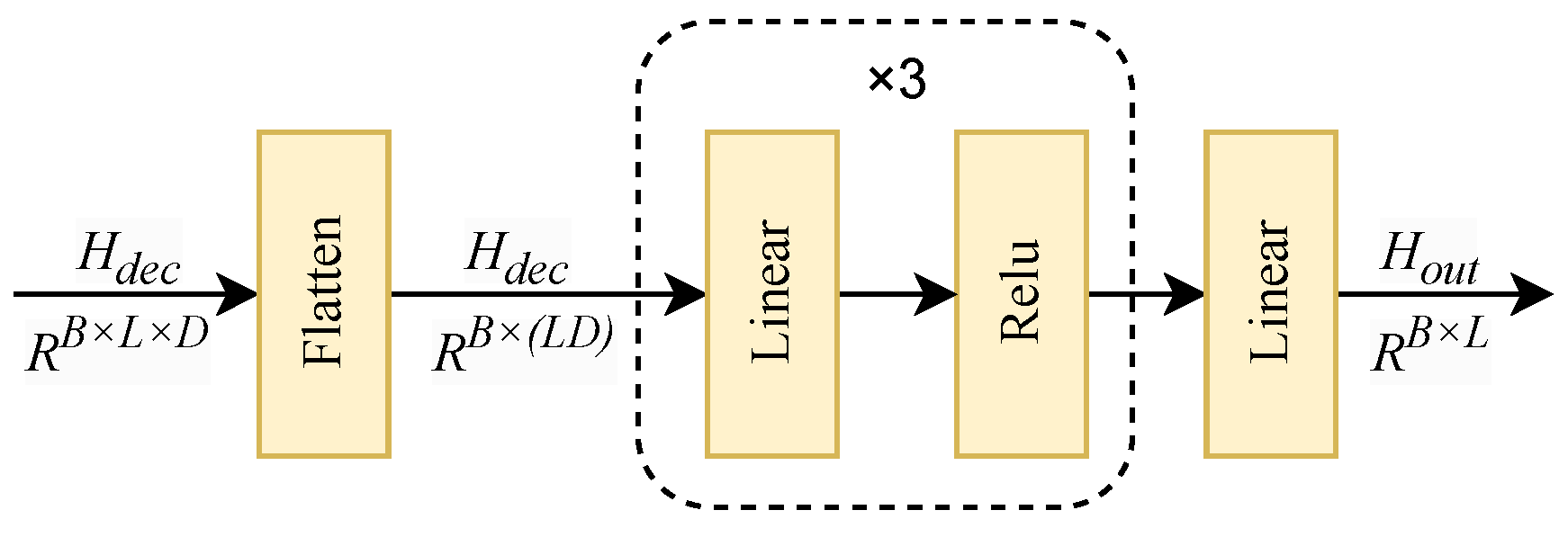
The model adopts a prediction head based on a multilayer perceptron (MLP) to generate the final output. The decoder output $H_{dec}$ has dimensions $[B, L, D]$, where B denotes the batch size, L the sequence length, and D the embedding dimension. The tensor $H_{dec}$ is flattened into a two-dimensional representation of size $[B, L\times D]$ and fed into the prediction head.

The prediction head consists of four fully connected layers with progressive dimensionality reduction. The first three layers employ a combination of linear transformation and ReLU activation to perform feature compression and abstraction. The ReLU activation introduces nonlinearity and sparse activation, enabling the model to retain salient temporal features while improving expressive capacity and computational efficiency. The final linear layer maps the transformed features to the target output dimension, producing the prediction result $H_{out}$ without additional nonlinear activation.

This lightweight MLP-based prediction head effectively translates high-level temporal representations into accurate output estimates, while maintaining robustness and stability in the presence of noise and incomplete observations commonly encountered in real-world air quality monitoring data.

The architecture of the prediction head module is illustrated in Figure 7.

2.4. Loss Function

During model training, a joint optimization objective is adopted by combining the mean squared error (MSE) loss and the information noise-contrastive estimation (InfoNCE) loss. This hybrid loss design enables the model to simultaneously improve reconstruction accuracy and learn discriminative latent representations through contrastive learning. By adjusting the relative weights of the two loss terms, the model can balance point-wise prediction fidelity and representation-level discrimination.

The MSE loss is used to measure the discrepancy between the predicted values and the corresponding ground-truth observations, and is defined as

$${\mathcal{L}}_{\mathrm{MSE}}={\displaystyle \frac{1}{N}}\sum _{i=1}^N{\left(Y_p\left(i\right)-Y_t\left(i\right)\right)}^2,$$

where $Y_p$ and $Y_t$ denote the predicted and true values, respectively, and N represents the number of samples.

To enhance representation learning under incomplete and unlabeled settings, the InfoNCE loss is incorporated as the contrastive learning objective. The InfoNCE loss encourages representations of positive sample pairs to be close in the embedding space, while pushing apart representations of negative samples. It is formulated as

$${\mathcal{L}}_{\mathrm{InfoNCE}}=-{\displaystyle \frac{1}{N}}\sum _{i=1}^{N}log{\displaystyle \frac{exp(\mathrm{sim}(q_i,k_i)/\tau )}{{\sum }_{j=1}^{M}exp(\mathrm{sim}(q_i,k_j)/\tau )}},$$

where $q_i$ denotes the anchor representation, $k_i$ is the corresponding positive sample, $k_j$ represents negative samples, and $\tau$ is a temperature parameter that controls the sharpness of the similarity distribution.

Unlike conventional cross-entropy objectives, the InfoNCE loss focuses on relative similarity relationships rather than absolute class labels. By maximizing mutual information between correlated samples and suppressing similarities with unrelated samples, it facilitates the learning of robust and discriminative feature representations. The use of multiple negative samples further improves generalization and mitigates overfitting.

The combined loss formulation is particularly suitable for air quality datasets collected from real-world sensor networks, where missing observations, noise contamination, and limited supervision are common. By jointly optimizing reconstruction accuracy and representation consistency, the proposed training objective enhances robustness and stability under realistic monitoring conditions.

2.5. Experimental Settings

The samples were divided chronologically into 70% training data, 10% validation data, and 20% test data. This study employed time series lengths of 24 h and 48 h, with varying missing ratios applied to each time series: (10%, 20%, 30%). During training, the encoder comprised 3 layers, the decoder 2 layers, and the prediction head featured 4 fully connected layers. The Adam optimizer was employed with a patience value of 5 rounds for early stopping. Batch size was set to 64, hidden vector size to 64, epoch size to 100, and the temperature coefficient of the loss function to 0.07. This study implemented the proposed model using the PyTorch (version 2.6.0) deep learning framework, with training and validation conducted on an NVIDIA GeForce RTX 3090 GPU. Other model parameters are summarized in

Table 1. Model parameters.

Parameters	Value
Sequence length	24 h, 48 h
Missing ratio	10%, 20%, 30%
Epoch	100
Batch size	64
Hidden size	64
Learning rate	0.001

.

3. Experiments and Analysis

3.1. Datasets

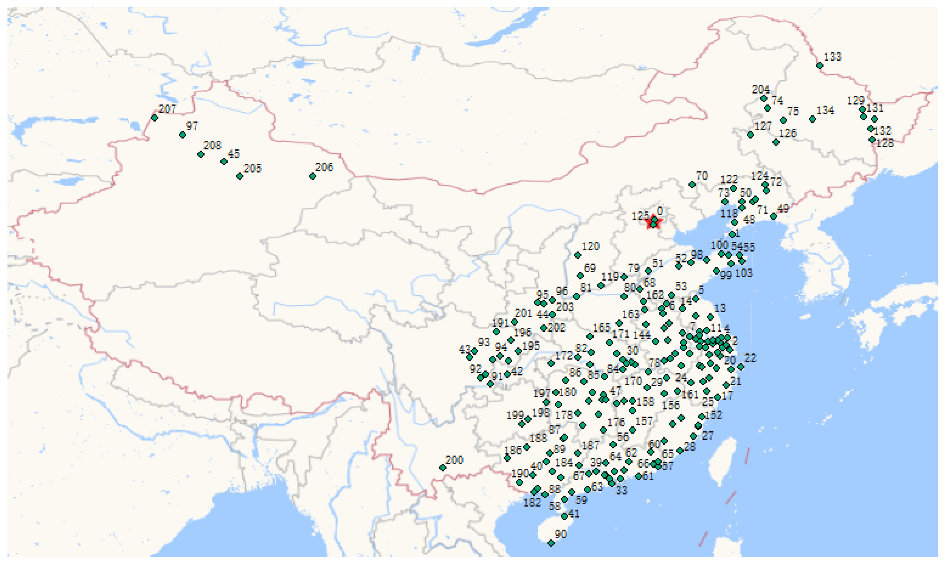
This paper evaluates the model’s performance using a Chinese air quality dataset. The dataset comprises air quality data from 209 monitoring stations across multiple regions in China. It includes meteorological information associated with each observation point throughout the observation period, covering key meteorological indicators such as temperature, precipitation, humidity, atmospheric pressure, wind speed, wind direction, and Air Quality Index (AQI). In addition, the dataset provides AQI records, which are used as the target variable for imputation and evaluation rather than as model input features. The dataset specifications are summarized in

Table 2. Dataset details.

Attribute	Value
Start Date	1 January 2017
End Date	30 May 2019
Number of Stations	209
Time Interval	1 h
Spatial Coverage	Nationwide
Number of Features	6
Primary Index	AQI

.

Note that AQI is treated as the prediction target, while only six meteorological variables are used as model inputs. The ranges of each feature are summarized in

Table 3. Feature range.

Feature	Min	Median	Mean	Max
Temperature (°C)	−20	16	15.8	50
Precipitation (mm)	0	0	12.7	300
Humidity (%)	0	54	56.1	100
Atmospheric pressure (hPa)	927	1008	988.4	1086
Wind speed (m/s)	0	2.8	3.2	50
Wind direction (°)	0	180	180	360
AQI	0	56	64.2	300

.

Table 3 summarizes the statistical ranges of all recorded feature variables in the dataset. Among them, AQI serves as the target variable for reconstruction, while the remaining six meteorological variables are used as input features.

The Air Quality Index (AQI) analyzed ranges from 0 to 300, providing a comprehensive assessment of overall ambient air quality. According to national classification schemes, the AQI is divided into six levels: Excellent (0–50), Good (51–100), Lightly Polluted (101–150), Moderately Polluted (151–200), and Heavily Polluted (201–300). This dataset does not include Severely polluted (301–500) levels. These levels reflect the progressive deterioration of health and environmental impacts and serve as the basis for assessing temporal variations and pollution events in this study. The level classifications are shown in

Table 4. Air quality levels.

Level	AQI	Gategory
1	0–50	Excellent
2	51–100	Good
3	101–150	Lightly Polluted
4	151–200	Moderately Polluted
5	201–300	Heavily Polluted
6	301–500	Severely polluted

.

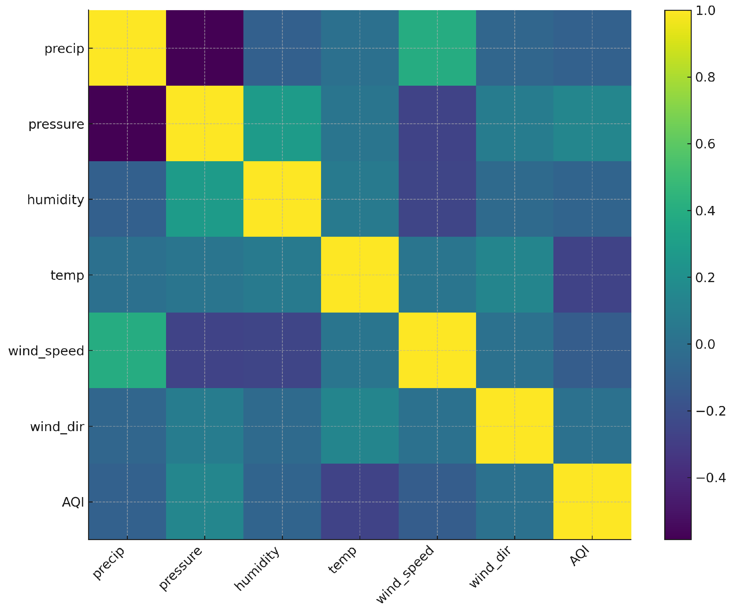
To further investigate the statistical characteristics of the dataset, a feature correlation heatmap was generated based on the Pearson correlation coefficients among all variables. As shown in Figure 8, the meteorological factors exhibit meaningful relationships with the AQI. In particular, show moderate positive correlations with AQI, suggesting that high-moisture or stable-pressure conditions may be associated with reduced pollutant dispersion. By contrast, wind speed displays a negative correlation with AQI, suggesting that stronger winds facilitate horizontal transport and dilution of air pollutants.

The heatmap also reveals that no pair of meteorological variables exhibits extremely high correlation (|r| > 0.9), indicating the absence of severe multicollinearity within the dataset. This confirms that all six meteorological variables provide non-redundant information and can be safely used as model inputs without additional dimensionality reduction. Overall, the correlation patterns are consistent with well-established atmospheric dispersion theory, validating both the reliability and physical coherence of the dataset.

The distribution of monitoring station locations is shown in Figure 9. Green dots mark the locations of air quality monitoring stations.

3.2. Training and Validation Analysis

During model training, to comprehensively evaluate the performance of the multi-task learning framework, we systematically monitored and analyzed the total loss and its individual component losses. The total loss function is composed of a weighted fusion of the mean squared error loss $L_{mse}$ and the information noise contrastive estimation loss $L_{infoNCE}$, expressed as

$$L_{total}=\alpha ·L_{mse}+\beta ·L_{infoNCE}$$

where $\alpha$ and $\beta$ denote the weighting coefficients for the reconstruction loss and the contrastive loss, respectively. In this study, the MSE loss serves as the primary optimization objective, as accurate reconstruction of continuous missing AQI values is the core task. The InfoNCE loss is incorporated as an auxiliary regularization term to guide representation learning and enhance feature discriminability.

The values of $\alpha$ and $\beta$ are empirically determined to maintain the dominance of the reconstruction objective while allowing the contrastive loss to contribute effectively during training. Specifically, $\alpha$ is set to 1 and $\beta$ is set to 0.2 throughout all experiments. This setting is chosen based on preliminary experiments, in which the reconstruction performance remains stable while the InfoNCE loss exhibits smooth convergence and enhances representation robustness without dominating the optimization process.

As can be seen from the overall loss curve in Figure 10a, both the training set loss and the validation set loss steadily decrease with the increase in iteration rounds, and tend to converge after about the 20th round. The validation set loss does not rebound, indicating that the training process is stable and no evident overfitting is observed. Further analysis of the loss structure reveals that the MSE loss in Figure 10b decreases rapidly in the early stages, indicating that the model effectively captures the main dynamic patterns of the time series; meanwhile, the InfoNCE loss in Figure 10c continuously decreases throughout the training process, reflecting that the model continuously optimizes feature embeddings through contrastive learning, enhancing the compactness of representations for positive sample pairs while increasing the separability from negative samples. The excellent convergence behavior of the total loss is the result of the combined effect of the predictive ability guaranteed by the MSE loss and the feature discrimination ability enhanced by the InfoNCE loss, thus verifying the rationality and effectiveness of the multi-task loss function designed in this paper from an experimental perspective.

3.3. Comparison with Baselines

To comprehensively evaluate the model’s performance, it is compared with the following baseline methods: Multi-Layer Perceptron (MLP), Long Short-Term Memory Network (LSTM), Informer, Conformer, Transformer, and Fedformer.

MLP: it is a feedforward neural network consisting of an input layer, one or more hidden layers, and an output layer. It uses nonlinear activation functions and backpropagation algorithms to learn complex input-output mapping relationships, making it one of the fundamental structures of deep learning.

LSTM: it is a special type of recurrent neural network that effectively captures long-term dependencies by introducing a “gating mechanism”, thereby solving the problems of gradient disappearance and gradient explosion that often occur in traditional RNNs when training long sequences.

Transformer: it is a deep learning model based on the self-attention mechanism, which can efficiently model global dependencies in sequences and avoid the long-term dependency issues of traditional RNNs. It is currently the core architecture for natural language processing and multimodal tasks.

Informer: it is an efficient time series prediction model based on the Transformer architecture, but it significantly reduces computational complexity through the ProbSparse self-attention mechanism and distillation operations, enabling it to maintain high prediction accuracy and efficiency when processing ultra-long sequences [23].

Conformer: it is a model that combines convolutional neural networks and Transformers, capable of modeling long-range dependencies while effectively capturing local features [24].

Fedformer: it proposes a hybrid expert architecture of a frequency-enhanced decomposed Transformer, introducing Fourier-enhanced blocks and wavelet-enhanced blocks in the Transformer structure to replace self-attention and cross-attention blocks [25].

The experimental results are presented in

Table 5. The 24 h filling effect of each model.

Method	10%				20%				30%
	MSE	MAE	RMSE	R2	MSE	MAE	RMSE	R2	MSE	MAE	RMSE	R2
MLP	0.2542	0.2085	0.5042	0.8497	0.2896	0.2398	0.5381	0.8193	0.3274	0.2701	0.5721	0.7992
LSTM	0.2283	0.1867	0.4778	0.8692	0.2657	0.2172	0.5155	0.8410	0.3029	0.2488	0.5504	0.8205
Informer	0.1951	0.1539	0.4416	0.8913	0.2258	0.1825	0.4753	0.8725	0.2583	0.2137	0.5082	0.8516
Conformer	0.1836	0.1452	0.4285	0.9005	0.2139	0.1734	0.4624	0.8816	0.2451	0.2046	0.4951	0.8603
Transformer	0.2053	0.1640	0.4531	0.8818	0.2377	0.1942	0.4876	0.8617	0.2695	0.2251	0.5190	0.8419
Fedformer	0.1675	0.1348	0.4093	0.9121	0.1973	0.1585	0.4442	0.8928	0.2286	0.1872	0.4781	0.8717
Our Model	0.1401	0.1121	0.3745	0.9307	0.1638	0.1292	0.4047	0.9114	0.1896	0.1483	0.4355	0.8896

and

Table 6. The 48 h filling effect of each model.

Method	10%				20%				30%
	MSE	MAE	RMSE	R2	MSE	MAE	RMSE	R2	MSE	MAE	RMSE	R2
MLP	0.3127	0.2584	0.5592	0.8304	0.3562	0.2983	0.5970	0.8107	0.4021	0.3387	0.6342	0.7905
LSTM	0.2805	0.2321	0.5297	0.8502	0.3268	0.2725	0.5718	0.8301	0.3724	0.3129	0.6102	0.8108
Informer	0.2398	0.1923	0.4897	0.8705	0.2786	0.2264	0.5279	0.8502	0.3182	0.2615	0.5641	0.8309
Conformer	0.2257	0.1816	0.4749	0.8807	0.2631	0.2147	0.5129	0.8604	0.3018	0.2503	0.5494	0.8406
Transformer	0.2521	0.2037	0.5021	0.8608	0.2924	0.2398	0.5410	0.8405	0.3329	0.2764	0.5770	0.8203
Fedformer	0.2059	0.1672	0.4537	0.8902	0.2437	0.1986	0.4937	0.8701	0.2815	0.2318	0.5306	0.8504
Our Model	0.1723	0.1395	0.4140	0.9105	0.2014	0.1628	0.4487	0.8903	0.2337	0.1892	0.4834	0.8709

below. As can be clearly observed from the tables, regardless of the sequence length (24 h or 48 h), when the data missing ratio is 10%, 20%, or 30%, the model achieves the best data filling performance across all three evaluation metrics. These improvements indicate that the proposed model can more effectively handle sensor interruptions and abrupt pollution episodes commonly encountered in real-world air quality monitoring, maintaining stable reconstruction performance even under high missing-rate conditions.

As shown in Figure 11, we selected the predicted values and actual values for the same 48-h time period from different models. It can be seen that the model can accurately predict the AQI values and their trends at most times. Compared with the predictions of other models, the prediction results of our model are significantly more accurate and have smaller errors.

3.4. Ablation Experiment

To validate the effectiveness of the modules, ablation experiments were conducted on the dataset using the model proposed in this paper. The data embedding module incorporating time-frequency domain feature mixing (TFDFM), the adaptive hierarchical attention module with global–local feature fusion (GLFF), and the multi-scale convolution module (MSTC) were introduced separately to demonstrate the impact of each module on the overall model. The experiments were conducted using a dataset with a 10% data missing rate. The experimental results are shown in

Table 7. The 24 h model module ablation experiment.

TFDFM	GLFF	MSTC	MSE	MAE
✗	✗	✗	0.1748	0.1388
✓	✗	✗	0.1712	0.1370
✗	✓	✗	0.1693	0.1319
✗	✗	✓	0.1709	0.1334
✓	✓	✗	0.1558	0.1256
✓	✗	✓	0.1576	0.1306
✗	✓	✓	0.1519	0.1244
✓	✓	✓	0.1401	0.1121

and

Table 8. The 48 h model module ablation experiment.

TFDFM	GLFF	MSTC	MSE	MAE
✗	✗	✗	0.1920	0.1531
✓	✗	✗	0.1851	0.1496
✗	✓	✗	0.1779	0.1433
✗	✗	✓	0.1798	0.1444
✓	✓	✗	0.1646	0.1361
✓	✗	✓	0.1669	0.1383
✗	✓	✓	0.1634	0.1345
✓	✓	✓	0.1602	0.1212

.

The results show that the data embedding module using time-frequency domain feature mixing (TFDFM), the adaptive hierarchical attention module using global–local feature fusion (GLFF), and the multi-scale convolution module (MSTC) each have a significant effect when used individually, and the effect is even better when used in pairs. When all three modules are used together, the results are optimal, effectively enhancing the model’s ability to transmit and capture deep time-frequency features, as well as its modeling capabilities for periodicity and frequency changes. This suggests that the overall performance gain arises from the complementary effects of multiple architectural components, rather than from any single module alone.

4. Conclusions

This paper proposes a contrastive learning-enhanced air quality data imputation framework that integrates unified time–frequency feature modeling, adaptive hierarchical attention, and multi-scale convolution to reconstruct long-term consecutive missing air quality data. A self-supervised contrastive learning strategy is designed to model realistic temporal correlations by operating on observed contextual subsequences surrounding missing segments, with data augmentation performed jointly in the time and frequency domains. The encoder combines global and local attention mechanisms with multi-scale temporal convolutions to capture long-range dependencies, local patterns, and nonlinear dynamics, while the decoder leverages self-attention and cross-attention to effectively integrate encoder representations for accurate reconstruction.

Extensive experiments conducted on real-world air quality datasets from multiple monitoring stations in China demonstrate the effectiveness of the proposed framework, particularly in reconstructing long-term consecutive missing observations under varying missing rates.

Building upon the proposed methodological design, the framework demonstrates strong potential for practical air quality data reconstruction tasks under scenarios involving missing or incomplete observations. By effectively learning robust temporal representations from partially observed time series, the model enhances the reliability of reconstructed AQI sequences under non-ideal monitoring conditions where data gaps are common. While the current study focuses on controlled missing-data settings, the proposed approach can potentially be extended to a broader range of real-world air quality monitoring applications, supporting downstream tasks such as environmental analysis, exposure assessment, and public health studies.

The proposed framework primarily focuses on modeling temporal dynamics and frequency-domain characteristics through a unified time–frequency learning architecture. Unlike approaches that explicitly rely on spatial correlation modeling, the proposed method does not incorporate dedicated spatial dependency modules and therefore does not require a large number of monitoring stations to operate effectively. As a result, the model remains applicable even in scenarios with a limited number of sampling stations, or when only single-station time-series data are available.

Regarding temporal resolution, the proposed model is mainly evaluated on hourly air quality time series, where both short-term temporal variations and frequency-domain patterns can be effectively captured. When applied to coarser time resolutions, such as daily observations, the framework remains applicable in principle; however, the reduction in temporal granularity may weaken the representation of high-frequency components in the frequency domain. In such cases, model performance may be affected, and appropriate adjustments to the temporal window size and multi-scale convolution settings would be required. Exploring adaptive strategies for different time lags will be considered in future work.

References

1. Marie, A.; Javar, N. Atmospheric pollution assessed by in situ measurement of magnetic susceptibility on lichens. Environ. Pollut. 2018, 235, 356–365. [Google Scholar] [CrossRef]
2. Chaparro, M.A.; Chaparro, M.A.; Castaneda-Miranda, A.G.; Marié, D.C.; Gargiulo, J.D.; Lavornia, J.M.; Natal, M.; Böhnel, H.N. Fine air pollution particles trapped by street tree barks: In situ magnetic biomonitoring. Environ. Pollut. 2020, 266, 115229. [Google Scholar] [CrossRef]
3. Liu, H.; Yan, G.; Duan, Z.; Chen, C. Intelligent modeling strategies for forecasting air quality time series: A review. Appl. Soft Comput. 2021, 102, 106957. [Google Scholar] [CrossRef]
4. Blu, T.; Thevenaz, P.; Unser, M. Linear interpolation revitalized. IEEE Trans. Image Process. 2004, 13, 710–719. [Google Scholar] [CrossRef]
5. Ma, Z.; Dey, S.; Christopher, S.; Liu, R.; Bi, J.; Balyan, P.; Liu, Y. A review of statistical methods used for developing large-scale and long-term PM2.5 models from satellite data. Remote Sens. Environ. 2022, 269, 112827. [Google Scholar] [CrossRef]
6. Ma, Z.; Hu, X.; Huang, L.; Bi, J.; Liu, Y. Estimating ground-level PM2.5 in China using satellite remote sensing. Environ. Sci. Technol. 2014, 48, 7436–7444. [Google Scholar] [CrossRef]
7. Masmoudi, S.; Elghazel, H.; Taieb, D.; Yazar, O.; Kallel, A. A machine-learning framework for predicting multiple air pollutants’ concentrations via multi-target regression and feature selection. Sci. Total. Environ. 2020, 715, 136991. [Google Scholar] [CrossRef] [PubMed]
8. Wahid, H.; Ha, Q.; Duc, H. Computational intelligence estimation of natural background ozone level and its distribution for air quality modelling and emission control. In Proceedings of the 28th International Symposium on Automation and Robotics in Construction (ISARC 2011), Seoul, Republic of Korea, 29 June–2 July 2011; pp. 551–557. [Google Scholar]
9. Kitagawa, Y.; Pedruzzi, R.; Galvão, E.; de Araújo, I.B.; de Almeida Alburquerque, T.T.; Kumar, P.; Nascimento, E.G.S.; Moreira, D.M. Source apportionment modelling of PM2.5 using CMAQ-ISAM over a tropical coastal-urban area. Atmos. Pollut. Res. 2021, 12, 101250. [Google Scholar] [CrossRef]
10. Thongthammachart, T.; Araki, S.; Shimadera, H.; Eto, S.; Matsuo, T.; Kondo, A. An integrated model combining random forests and WRF/CMAQ model for high accuracy spatiotemporal PM2.5 predictions in the Kansai region of Japan. Atmos. Environ. 2021, 262, 118620. [Google Scholar] [CrossRef]
11. Nieto, P.; Lasheras, F.; García-Gonzalo, E.; de Cos Juez, F.J. PM10 concentration forecasting in the metropolitan area of Oviedo (Northern Spain) using models based on SVM, MLP, VARMA and ARIMA: A case study. Sci. Total. Environ. 2018, 621, 753–761. [Google Scholar] [CrossRef] [PubMed]
12. He, Z.; Liu, P.; Zhao, X.; He, X.; Liu, J.; Mu, Y. Responses of surface O3 and PM2.5 trends to changes of anthropogenic emissions in summer over Beijing during 2014–2019: A study based on multiple linear regression and WRF-Chem. Sci. Total. Environ. 2022, 807, 150792. [Google Scholar] [CrossRef]
13. Rodríguez-Trejo, A.; Böhnel, H.N.; Ibarra-Ortega, H.E.; Salcedo, D.; González-Guzmán, R.; Castañeda Miranda, A.G.; Sánchez-Ramos, L.E.; Chaparro, M.A.E.; Chaparro, M.A.E. Air Quality Monitoring with Low-Cost Sensors: A Record of the Increase of PM2.5 during Christmas and New Year’s Eve Celebrations in the City of Queretaro, Mexico. Atmosphere 2024, 15, 879. [Google Scholar] [CrossRef]
14. Zhang, B.; Rong, Y.; Yong, R.; Qin, D.; Li, M.; Zou, G.; Pan, J. Deep learning for air pollutant concentration prediction: A review. Atmos. Environ. 2022, 290, 119347. [Google Scholar] [CrossRef]
15. Rijal, N.; Gutta, R.; Cao, T.; Lin, J.; Bo, Q.; Zhang, J. Ensemble of deep neural networks for estimating particulate matter from images. In Proceedings of the 2018 IEEE 3rd international conference on image, Vision and Computing (ICIVC), Chongqing, China, 27–29 June 2018; pp. 733–738. [Google Scholar]
16. Loy-Benitez, J.; Vilela, P.; Li, Q.; Yoo, C. Sequential prediction of quantitative health risk assessment for the fine particulate matter in an underground facility using deep recurrent neural networks. Ecotoxicol. Environ. Saf. 2019, 169, 316–324. [Google Scholar] [CrossRef]
17. Li, Y.; Gan, Z.; Shen, Y.; Liu, J.; Cheng, Y.; Wu, Y.; Carin, L.; Carlson, D.; Gao, J. StoryGAN: A Sequential Conditional GAN for Story Visualization. In Proceedings of the IEEE/CVF Conference on Computer Vision and Pattern Recognition (CVPR); IEEE: New York, NY, USA, 2019; pp. 6329–6338. [Google Scholar]
18. Yan, R.; Liao, J.; Yang, J.; Sun, W.; Nong, M.; Li, F. Multi-hour and multi-site air quality index forecasting in Beijing using CNN, LSTM, CNN-LSTM, and spatiotemporal clustering. Expert Syst. Appl. 2021, 169, 114513. [Google Scholar] [CrossRef]
19. Liang, Y.; Xia, Y.; Ke, S.; Wang, Y.; Wen, Q.; Zhang, J.; Zheng, Y.; Zimmermann, R. Airformer: Predicting nationwide air quality in China with transformers. In Proceedings of the AAAI Conference on Artificial Intelligence, Washington, DC, USA, 7–14 February 2023; Volume 37, pp. 14329–14337. [Google Scholar]
20. Tolstikhin, I.; Housby, N.; Kolesnikov, A.; Beyer, L.; Zhai, X.; Unterthiner, T.; Yung, J.; Steiner, A.; Keysers, D.; Uszkoreit, J.; et al. MLP-Mixer: An all-MLP Architecture for Vision. arXiv 2021, arXiv:2105.01601. [Google Scholar]
21. Vaswani, A.; Shazeer, N.; Parmar, N.; Uszkoreit, J.; Jones, L.; Gomez, A.; Kaiser, U.; Polosukhin, I. Attention is All You Need. Adv. Neural Inf. Process. Syst. 2017, 30. [Google Scholar]
22. Han, K.; Wang, Y.; Chen, H.; Chen, X.; Guo, J.; Liu, Z. A Survey on Vision Transformer. IEEE Trans. Pattern Anal. Mach. Intell. 2023, 45, 87–110. [Google Scholar] [CrossRef]
23. Zhou, H.; Zhang, S.; Peng, J.; Zhang, S.; Li, J.; Xiong, H.; Zhang, W. Informer: Beyond Efficient Transformer for Long Sequence Time-Series Forecasting. In Proceedings of the AAAI Conference on Artificial Intelligence, AAAI, Virtually, 2–9 February 2021; Volume 35, p. 17325. [Google Scholar] [CrossRef]
24. Gulati, A.; Qin, J.; Chiu, C.C.; Parmar, N.; Zhang, Y.; Yu, J.; Han, W.; Wang, S.; Zhang, Z.; Wu, Y.; et al. Conformer: Convolution-augmented Transformer for Speech Recognition. In Proceedings of the Interspeech 2020, ISCA, ICLR, Shanghai, China, 25–29 October 2020; pp. 5036–5040. [Google Scholar] [CrossRef]
25. Zhou, T.; Ma, Z.; Wen, Q.; Wang, X.; Sun, L.; Jin, R. FEDformer: Frequency Enhanced Decomposed Transformer for Long-term Series Forecasting. In Proceedings of the 39th International Conference on Machine Learning, Baltimore, MD, USA, 17–23 July 2022; Proceedings of Machine Learning Research; Chaudhuri, K., Jegelka, S., Song, L., Szepesvari, C., Niu, G., Sabato, S., Eds.; PMLR: London, UK, 2022; Volume 162, pp. 27268–27286. [Google Scholar]
26. Kitaev, N.; Kaiser, L.; Levskaya, A. Reformer: The Efficient Transformer. arXiv 2020. [Google Scholar] [CrossRef]
27. Wu, H.; Xu, J.; Wang, J.; Long, M. Autoformer: Decomposition Transformers with Auto-Correlation for Long-Term Series Forecasting. arXiv 2021. [Google Scholar] [CrossRef]
28. Samal, K.; Babu, K.; Das, S. Multi-directional temporal convolutional artificial neural network for PM2.5 forecasting with missing values: A deep learning approach. Urban Clim. 2021, 36, 100800. [Google Scholar] [CrossRef]
29. Horn, S.A.; Dasgupta, P.K. The Air Quality Index (AQI) in historical and analytical perspective: A tutorial review. Talanta 2023, 265, 125260. [Google Scholar] [CrossRef] [PubMed]
30. Liu, J.; Chen, S. TimesURL: Self-Supervised Contrastive Learning for Universal Time Series Representation Learning. In Proceedings of the AAAI Conference on Artificial Intelligence, AAAI, Vancouver, BC, Canada, 26–27 February 2024; Volume 38. [Google Scholar] [CrossRef]
31. Lee, S.; Park, T.; Lee, K. Soft Contrastive Learning for Time Series. In Proceedings of the International Conference on Learning Representations (ICLR), Vienna, Austria, 7–11 May 2024. [Google Scholar]
32. Chen, M.; Xu, Z.; Zeng, A.; Xu, Q. FrAug: Frequency Domain Augmentation for Time Series Forecasting. arXiv 2023, arXiv:2302.09292. [Google Scholar] [CrossRef]
Figure 1. Division of positive and negative samples.
Information 17 00121 g001
Figure 2. Model structure.
Information 17 00121 g002
Figure 3. Data embedding layer.
Information 17 00121 g003
Figure 4. Adaptive hierarchical attention module.
Information 17 00121 g004
Figure 5. Multi-head attention mechanism data process.
Information 17 00121 g005
Figure 6. Multi-scale temporal convolution module.
Information 17 00121 g006
Figure 7. Prediction head module.
Information 17 00121 g007
Figure 8. Correlation matrix among meteorological variables and AQI.
Information 17 00121 g008
Figure 9. Air quality monitoring station distribution map.
Information 17 00121 g009
Figure 10. Training and validation loss.
Information 17 00121 g010
Figure 11. The 48 h reconstruction values for each model.
Information 17 00121 g011