Abstract
This study introduces a fully uncertainty-aware forecasting framework for NBA games that integrates team-level performance metrics, rolling-form indicators, and spatial shot-chart embeddings. The predictive backbone is a recurrent neural network equipped with Monte Carlo dropout, yielding calibrated sequential probabilities. The model is evaluated against strong baselines including logistic regression, XGBoost, convolutional models, a GRU sequence model, and both market-only and non-market-only benchmarks. All experiments rely on strict chronological partitioning (train ≤ 2022, validation 2023, test 2024), ablation tests designed to eliminate any circularity with bookmaker odds, and cross-season robustness checks spanning 2012–2024. Predictive performance is assessed through accuracy, Brier score, log-loss, AUC, and calibration metrics (ECE/MCE), complemented by SHAP-based interpretability to verify that only pre-game information influences predictions. To quantify economic value, calibrated probabilities are fed into a frictionless betting simulator using fractional-Kelly staking, an expected-value threshold, and bootstrap-based uncertainty estimation. Empirically, the uncertainty-aware model delivers systematically better calibration than non-Bayesian baselines and benefits materially from the combination of shot-chart embeddings and recent-form features. Economic value emerges primarily in less-efficient segments of the market: The fused predictor outperforms both market-only and non-market-only variants on moneylines, while spreads and totals show limited exploitable edge, consistent with higher pricing efficiency. Sensitivity studies across Kelly multipliers, EV thresholds, odds caps, and sequence lengths confirm that the findings are robust to modelling and decision-layer perturbations. The paper contributes a reproducible, decision-focused framework linking uncertainty-aware prediction to economic outcomes, clarifying when predictive lift can be monetized in NBA markets, and outlining methodological pathways for improving robustness, calibration, and execution realism in sports forecasting.
1. Introduction
Sports betting has expanded rapidly over the past decade, driven by digital platforms, liberalisation, and the integration of data analytics into pricing and risk management. Global revenues exceeded USD 100 billion in 2024, with compound annual growth projections above 8%, and the United States alone is expected to surpass USD 160 billion by 2033 [1]. Such growth has been accompanied by increased household exposure and documented financial risk, including higher bankruptcy incidence in newly legalised jurisdictions [2]. These trends motivate the development of transparent, data-driven frameworks for probabilistic forecasting and risk-aware wagering strategies.
Modern betting markets represent the culmination of a long historical trajectory. From early wagering practices in ancient Egypt and Greece to the formalisation of odds-based bookmaking in eighteenth-century Britain, the central principle has remained the quantification of uncertainty. Contemporary markets rely primarily on decimal and American odds, whose implied probabilities are given by
These market-derived probabilities summarise bookmaker assessments based on large information sets and typically exhibit a high degree of efficiency. However, efficiency in this context is not equivalent to perfection: small, structured discrepancies between market-implied probabilities and well-calibrated model estimates may still arise and, when present, are directly relevant for value-based decision rules.
Regulatory regimes differ across jurisdictions—such as the UK Gambling Commission’s consumer-protection framework, the German Interstate Treaty’s licensing structure, or the heterogeneous US landscape post-PASPA repeal—yet the analytical challenge remains the same: markets aggregate information rapidly, and any economically actionable signal must reflect non-redundant deviations from those aggregated expectations. Characterising when such deviations exist, and how uncertainty-aware models can exploit them under realistic wagering constraints, therefore forms a central concern.
Despite substantial interest in machine learning for sports forecasting, two methodological gaps remain salient. First, much of the literature emphasises classification accuracy, whereas value-based decision-making depends critically on calibrated probabilities. Calibration-oriented studies do exist (e.g., [3]), but they typically do not combine calibration with spatial modelling, uncertainty quantification, and decision-layer analysis. Second, the connection between predictive performance and economic outcomes is often left implicit, limiting understanding of how uncertainty interacts with execution constraints such as stake limits, odds ceilings, and expected-value thresholds. Large-sample analyses (e.g., [4]) further indicate that profitability in NBA markets is limited unless models incorporate informative features not fully internalised by bookmakers.
This study addresses these gaps through three contributions. First, we develop an uncertainty-aware forecasting pipeline for NBA games that integrates structured box-score statistics, market-derived features, and spatial shot-chart embeddings encoded by a convolutional neural network. All inputs are constructed strictly from pre-game information, including closing odds and lagged rolling indicators. Second, we pair the resulting calibrated predictive distributions with a decision layer based on fractional-Kelly staking and expected-value filtering, providing a transparent mapping from probabilistic lift to economic performance under realistic constraints. Third, we evaluate predictive and financial performance not only for moneyline markets but also for spreads and totals, and we analyse transferability to player-level propositions (under synthetic odds) and to other professional basketball leagues. This broader evaluation situates the results within ongoing debates on market efficiency and cross-domain signal persistence.
These contributions are guided by two research questions:
- To what extent can calibrated, uncertainty-aware models identify and exploit the small but potentially persistent deviations from market-implied probabilities that arise in NBA betting markets, and in which market segments are such deviations most likely to occur?
- How do fractional-Kelly staking, expected-value thresholds, and explicit predictive uncertainty shape the translation of probabilistic lift into long-run bankroll dynamics?
To preview the methodological approach (depicted in Figure 1), we integrate (i) team-level, lagged-form, and spatial features derived from historical pre-game information; (ii) sequential modelling via a recurrent neural network with Bayesian regularisation; and (iii) chronological train–validation–test splits to avoid leakage. Betting simulations adopt realistic constraints (stake caps, EV thresholds, and odds ceilings) and illustrate how calibrated probabilities interact with selective wagering.
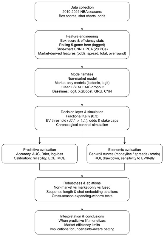
Figure 1.
Research workflow: from data collection and feature engineering to modelling, decision layer, evaluation, robustness analysis, and conclusions.
The remainder of this paper is organised as follows: Section 2 situates the contribution within the literature on sports forecasting, calibration, and decision-theoretic staking. Section 3 reviews probabilistic modelling, calibration, and market structure. Section 4 describes the data pipeline, feature engineering, predictive architecture, and decision layer. Section 5 analyses results across market segments and leagues. Section 6 concludes with limitations and directions for future research.
2. Related Work
Sports-betting prediction has evolved into a mature interdisciplinary domain spanning statistical modelling, machine learning, and the study of market microstructure. Since bookmaker prices reflect large information sets and strategic adjustments, empirical evaluation must consider not only classification accuracy but also probability calibration, execution realism, and economic usefulness. Recent contributions converge on the view that predictive lift acquires value only when paired with robust calibration, transparent decision rules, and realistic odds assumptions. Within this broader landscape, prior work can be organised into three complementary strands: calibration-aware forecasting, discriminative modelling using structured features, and market-aware economic evaluation.
A first strand emphasises probability calibration as a determinant of betting profitability. Walsh and Joshi [3], building on critiques of accuracy-only evaluation [5], compare accuracy-based versus calibration-based model-selection pipelines across NBA seasons 2014–2019. Their models—logistic regression, random forests, SVMs, and multilayer perceptrons—are trained on pre-game box-score features and are evaluated against Westgate closing moneylines. Calibration-selected pipelines consistently achieve higher ROI under both fixed-stake and fractional-Kelly sizing, showing that probability reliability affects economic outcomes even when classification metrics are comparable. However, this work does not incorporate spatial representation learning, sequential models, or explicit uncertainty quantification, and does not examine how calibrated probabilities interact with real-world execution constraints.
A second strand investigates discriminative performance using structured team and player statistics. Wang [6] evaluates logistic regression, SVMs, random forests, and feed-forward neural networks on more than 25,000 NBA games (2004–2020), using leakage-controlled shooting efficiency, turnover, rebounding, and assist features. Random forests and deep networks achieve the strongest accuracy and AUC, confirming that these structured metrics carry predictive signal. Yet the study does not assess calibration or simulate betting performance, leaving unclear whether discriminative lift survives bookmaker pricing or translates into value.
Adam, Pantatosakis, and Tsagris [7] extend this line of research to within-game prediction using half-time features for 3540 NBA games (2020–2023). Ten algorithms (CART, kNN, SVMs, neural networks, naïve Bayes, GBM, XGBoost, and logistic regression) are compared using repeated cross-validation [8,9] and greedy ensembling [5]. Ensembles reach AUCs above 0.90 within season but decline to 0.78–0.80 across seasons, highlighting temporal drift. Their analysis includes SHAP and ALE interpretability but does not address pre-game probability calibration, predictive uncertainty, or betting outcomes. Although neural networks are used, they function as standard discriminative classifiers rather than as spatial or sequential representation learners.
A third strand examines market realism, odds dynamics, and the feasibility of executing profitable strategies. Zimmermann [4] compares naïve Bayes, neural networks, random forests, and a Pomeroy-style model across NBA, NCAA, and NFL games from 2015 to 2018 using least-favourable prices from Vegas Insider. Despite comparable accuracy across models, realised profits vary substantially by sport: The NFL and NCAA show occasional exploitable inefficiencies, whereas NBA markets appear considerably tighter. This work underscores that profitability requires both calibrated signals and market-aware decision rules, and that accuracy alone is insufficient in markets with limited inefficiency. However, the study does not incorporate uncertainty quantification, probability calibration, or bankroll-optimising decision layers.
Across these strands, three insights recur. First, calibration materially affects ROI, whereas accuracy alone provides an incomplete measure of decision usefulness. Second, market realism shapes outcomes: Adverse price selection, liquidity constraints, and season–boundary drift all influence realised profitability. Third, existing models—whether discriminative (Wang [6]) or within-game (Adam et al. [7])—do not integrate spatial embeddings, sequential uncertainty estimation, and financially coherent decision rules within a single pre-game forecasting pipeline.
Despite substantial progress, no prior work jointly integrates (i) high-resolution pre-game spatial embeddings derived from shot chart heatmaps, (ii) recurrent neural architectures with Monte Carlo dropout for calibrated uncertainty over sequential form indicators, and (iii) an explicit, market-aware decision layer based on expected-value thresholds and fractional-Kelly staking evaluated under strict chronological splits.
The present study fills this gap by combining structured statistics, PCA-refined spatial embeddings, and market-derived features with a Bayesian RNN whose predictive distributions feed directly into a transparent bankroll simulation. This unified design links representation learning, uncertainty quantification, and decision-theoretic wagering within a single coherent framework, enabling a clearer assessment of when—and under which market conditions—probabilistic lift translates into economic value.
Table 1 summarizes the strengths and limitations of the ost relevant articles.

Table 1.
Comparison of selected studies in US sports prediction, emphasising calibration, uncertainty quantification, and decision-aware wagering.
3. Background
Convolutional neural networks (CNNs) and recurrent neural networks (RNNs) are the core components of the proposed forecasting pipeline. CNNs provide inductive biases suited to spatial structure, while RNNs model sequential dependencies in team form indicators. This section summarises the mathematical principles underlying both architectures in a manner consistent with the feature engineering and modelling choices adopted later.
3.1. Convolutional Neural Networks
CNNs encode spatial locality through three mechanisms: local connectivity, weight sharing, and hierarchical feature composition [10]. Their biological motivation traces back to the work of Hubel and Wiesel on orientation-selective cortical neurons [11]. Algorithmically, CNNs exploit structured filters applied across spatial positions to extract increasingly abstract representations [12].
Let the input to layer l be
where , , and denote height, width, and channels. A convolutional layer uses a filter bank
where is the kernel size and the number of output channels. The output tensor is produced by discrete cross-correlation (the operation typically called “convolution” in deep learning):
With stride and zero-padding , the output spatial dimensions are
“Same” padding corresponds to , chosen so that and for unit stride.
Regarding quivariance and invariance, Let denote a spatial translation. Convolution satisfies the translation-equivariance identity:
Downsampling operations break equivariance but promote approximate invariance, aligning the learned representation with tasks insensitive to small input shifts.
Concerning activation and normalization, channel-wise nonlinearities are applied as
Normalization layers (batch, layer, or instance normalization) stabilise the distribution of pre-activations and aid optimization.
For general kernel sizes , strides , and paddings , the effective stride and receptive field along height obey the recurrences
Analogous equations hold for width. These relations quantify the spatial context available to each unit.
Concerning the pooling step, given stride and window , max- and average-pooling are
Both operators are nonexpansive under and, for average pooling, also under , providing robustness to high-frequency perturbations.
After global pooling, a dense layer feeds a softmax
with cross-entropy loss
3.2. Recurrent Neural Networks
RNNs process sequences by maintaining a hidden state [13,14]. A standard Elman RNN with input , hidden state , and output satisfies
where is typically tanh or ReLU.
Let be the sequence loss and define pre-activations
The Jacobian at step u is
The gradient with respect to is
For tanh activations, the spectral radius determines vanishing () or exploding () gradients. For ReLU activations, , so vanishing arises from dead units and exploding from unbounded accumulation of active paths.
3.3. Long Short-Term Memory Networks
LSTMs augment RNNs with gated memory [15]. With input , hidden state , and cell state :
with updates
The nearly identity gradient path through when mitigates vanishing gradients over long horizons. The parameter count is
which is exactly four times that of a simple RNN of the same width.
Table 2 recaps the strengths and limitations of the discussed deep learning models.
Table 2.
Selected strengths and limitations of CNN and LSTM families.
4. Models and Experiments
We assemble an integrated dataset linking official game statistics, spatial shot information, and betting-market data so as to capture both on-court performance and the off-court expectations embedded in odds. Game-level statistics are scraped from Basketball Reference for seasons 2010–2024 via a Playwright + BeautifulSoup pipeline that iterates monthly schedules and retrieves box-score pages to local HTML with retries and backoff. Parsed tables are converted with pandas into structured records combining line scores, team box-score aggregates, and advanced efficiency indicators. For each game, we merge home and away features so that each team appears once with opponent-adjusted attributes.
Spatial shot charts are rasterized into 2D heatmaps on a fixed grid and are passed through a convolutional encoder with three convolution pool blocks, adaptive average pooling, and a final dense layer. The encoder outputs a 128-dimensional embedding that captures court space usage, shot density, and spatial diversity (e.g., perimeter versus paint frequency, corner threes versus above-the-break usage). As raw, 128-dimensional embeddings are high-dimensional and noisy, we apply principal component analysis (PCA) fitted strictly on the training set: Embeddings from seasons 2010–2018 are stacked into a matrix, PCA is fitted, and the transformation is then frozen. PCA reduces the representation to principal components, which retain 92.7% of the variance and empirically improve calibration and stability relative to unreduced embeddings. Retaining components increases explained variance to 96.1% but does not materially improve validation log-loss or AUC. In the final model, the PCA-reduced embedding is concatenated with box-score and market-derived features before being fed to the recurrent module.
To quantify the contribution of PCA, we compare three variants: (i) raw 128-dimensional embeddings, (ii) PCA-20 (92.7% variance explained), and (iii) PCA-30 (96.1% variance explained). PCA-20 achieves the best calibration and lowest validation log-loss, while PCA-30 yields only marginal AUC gains at the cost of worse calibration. Raw embeddings are computationally heavier and produce higher variance across validation seasons, consistent with overparameterisation relative to the available sequence length. Overall, the CNN encoder plus PCA-refined embeddings provide spatial and stylistic information in a compact representation that integrates cleanly into the forecasting pipeline.
For each team we compute rolling performance indicators over the last five completed games, using exclusively past information to avoid lookahead bias. For a match between teams A and B played on date t, the window for team A is the set of its five most recent games strictly preceding t; likewise for team B. All rolling statistics (shooting percentages, rebounds, assists, turnovers, pace, and efficiency measures) are therefore lagged features. The construction is symmetric: Both teams receive their own five-game aggregates, and the model is fed the pair aligned on the match date. If a team has fewer than five previous games (season start), the observation is excluded from sequence models that require at least five time steps to preserve consistent temporal structure. For use in tabular baselines, these rolling windows are summarised into scalar indicators such as team_rolling_win_rate_5 (mean of the binary outcome won over the last five games) and team_rolling_pts_5 (mean points scored), both computed with a one-step temporal shift so that only games strictly preceding t are used.
Moneylines, spreads, and totals are collected from a public Kaggle dataset (uploaded by Christopher Treasure as NBA odds data; visited 29 August 2025; https://www.kaggle.com/datasets/christophertreasure/nba-odds-data) and, where missing, from major outlets (CBS Sports, Action Network, FoxSports, USAToday). American-odds moneylines are converted to decimal odds and implied probabilities
and
We compute the overround
which measures the bookmaker margin. For a team-centric representation, we define
and
and include the scalar features implied_prob_team (), spread, total, and overround () in the input vector. These quantities summarise market assessments of relative strength, expected scoring level, and bookmaker edge, and they are crucial for value-based betting decisions.
We augment team records with pace, projected possessions, point differential, and game totals, and compute rolling five-game averages as described above to capture short-term form. Headline-based sentiment scores (ESPN/Yahoo via Google News) were evaluated but showed weak association with outcomes and odds movements; they are excluded from the final feature set. The resulting panel links (i) parsed box scores, (ii) PCA-20 shot-location embeddings, and (iii) market-adjusted probabilities into a unified pre-game feature vector for each team game.
League style evolves markedly over 2010–2024. Three-point attempts roughly double and display a sustained upward drift (Figure 2), while average points per game increase in parallel (Figure 3).
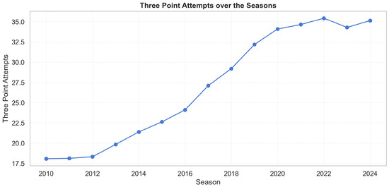
Figure 2.
Three-point attempts per game by season (2010–2024). The monotonic rise supports the use of era normalization.
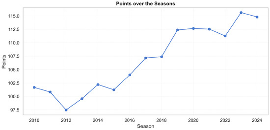
Figure 3.
Average points per game by season (2010–2024). Rising totals mirror the increase in perimeter volume and pace.
Figure 4 and Figure 5 highlight deeper structural change. In Figure 4, the offensive-rating distribution (points scored per 100 possessions) shifts rightwards and becomes more concentrated over time, indicating higher median scoring efficiency and reduced dispersion, consistent with league-wide adoption of pace-and-space offences, increased three-point volume, and rule changes favouring perimeter freedom of movement. The right tail thickens after 2018, reflecting historically elite offences. Figure 5 shows an analogous rightward shift in defensive ratings (points allowed per 100 possessions). The increase in defensive ratings reflects offensive inflation rather than uniformly weaker defence: It becomes harder to maintain low ratings when league scoring rises. The widening of the distribution suggests greater volatility in defensive outcomes, as teams face a more diverse mix of offensive styles. Taken together, the two figures show a joint upward drift in both offensive and defensive efficiency, indicating that the modern NBA environment is fundamentally different from earlier seasons. This motivates era controls and standardization. Accordingly, all raw counts are expressed per 100 possessions to remove pace effects, and season-fixed effects (or z-normalization within season) are used to ensure comparability across years.
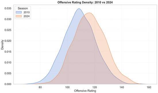
Figure 4.
Offensive rating densities for 2010 vs. 2024. The rightward shift indicates higher offensive efficiency in 2024.
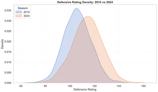
Figure 5.
Defensive rating densities for 2010 vs. 2024. The rightward shift reflects more points allowed in 2024; distributions still overlap, so normalization rather than hard stratification is appropriate.
We initially framed outcome prediction as regression (team points) using sequences of prior games processed by an LSTM; although this captured scoring dynamics, RMSE remained too large for reliable winner inference. We therefore adopted binary classification for win/loss using the same sequential inputs (rolling statistics and PCA-reduced embeddings) over the last five games. To preserve causality, data are split chronologically: training on seasons ≤ 2022, validation on 2023, and testing on 2024. The main win model is an LSTM-based architecture with Monte Carlo (MC) dropout at inference, providing calibrated probabilities and uncertainty estimates that are crucial for principled betting decisions. We extend modelling to spread (cover/no-cover) and totals (over/under) using the same feature space. Targets are defined by comparing observed outcomes to bookmaker lines from each team’s perspective. To measure the value of temporal context, we compare recurrent models to feed-forward MLPs under identical features and splits. Evaluation emphasises discrimination (accuracy, ROC–AUC), probabilistic quality (Brier score, log-loss), and confusion matrices to monitor class balance and calibration.
Economic value is assessed using a fractional-Kelly staking rule [20]. For decimal odds o and win probability p (with ), the full Kelly fraction is
To control risk, we use 0.3-Kelly, enforce a minimum expected-value threshold (), and impose a per-bet limit of EUR 100, with odds capped at 10.0. MC-dropout yields a distribution of predicted probabilities; wagers are placed only when both Kelly and criteria hold, filtering for edge and confidence. Bankroll simulations start at EUR 100 and proceed sequentially through the 2024 schedule; we record the full equity curve, number of bets, hit rate, and standard risk diagnostics (e.g., maximum drawdown). The same staking protocol is reused for all comparative baselines.
Uncertainty-aware win models (LSTM + MC-dropout) produce a steadily increasing equity curve on NBA moneylines (Figure 6).
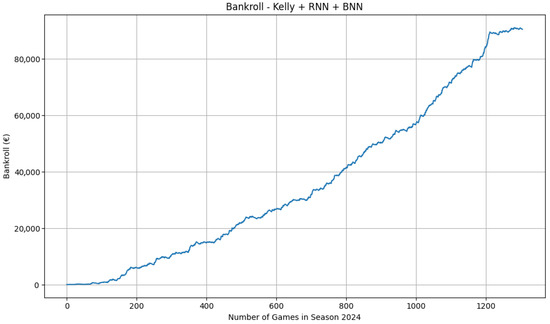
Figure 6.
NBA moneyline bankroll, test season 2024. Protocol: chronological evaluation, 0.3-Kelly, , stake cap EUR 100, starting bankroll EUR 100.
Periods of faster growth alternate with plateaus and shallow drawdowns, consistent with (i) time-varying edge, (ii) the selection filter reducing action during low-confidence windows, and (iii) the interaction between the Kelly fraction and the per-bet cap. Spread models are neutral to mildly negative, and totals deliver only marginal gains, aligning with the view that those markets are more efficient.
Table 3 compares several mainstream baselines on the 2024 test season under the same chronological split and staking rules. The market-implied probabilities and the logistic regression baseline exhibit reasonable calibration but do not generate profit, with final bankrolls of EUR 100 and EUR 80.34 respectively. Logistic regression attains the best Brier score and log-loss among tabular baselines (0.199 and 0.583), but its value-based filter yields a modest number of bets and a negative ROI. XGBoost offers slightly worse probabilistic scores (Brier 0.202, log-loss 0.589) but higher AUC (0.754, not shown in the table) and, critically, the best economic performance among tabular models, with a final bankroll of EUR 143.76 (ROI ) over 36 bets (hit rate 0.389). This illustrates that small differences in probability quality can interact non-linearly with the staking and EV thresholds, producing different economic outcomes. The GRU sequence model ingests a longer form history (last ten games per team) and achieves lower accuracy (0.604) and weaker probabilistic metrics than the tabular baselines. Its calibration is poor, and it issues many low-value bets, leading to aggressive overbetting: 1047 wagers, hit rate 0.284, and complete bankroll loss (ROI ). Finally, a CNN trained on shot location heatmaps and the same tabular features does not outperform simpler tabular baselines (accuracy 0.53, log-loss 0.694, AUC 0.462), suggesting that in the present configuration, deep spatial representation alone is insufficient to extract an edge over the market.
Table 3.
Comparison of baseline models on the 2024 test season. Final bankroll (BK) is computed using identical Kelly-based staking rules (fractional Kelly , EV , EUR 100 maximum stake, odds cap ) for the models where betting simulation was performed.
Figure 6 reports the bankroll trajectory obtained using our main model, which grows substantially over time (final bankroll ). To verify that this growth does not arise from compounding artefacts, unrealistic odds, or the staking mechanism itself, we evaluate two baseline systems under the same betting conditions used in the main experiment (fractional Kelly 0.3, EV , EUR 100 stake cap, odds cap 10.0), starting from the same initial capital of EUR 100. When replacing our model probabilities with the probabilities implied by the decimal odds (), the strategy places virtually no bets and the bankroll remains equal to the initial €100 (ROI ). A sensitivity analysis over 48 combinations of Kelly multiplier, EV threshold, stake cap, and odds cap yields final bankroll values consistently equal to EUR 100, and a block bootstrap produces a degenerate distribution with median EUR 100 and 2.5–97.5 percentiles [EUR 100, EUR 100]. This confirms that the staking engine alone cannot generate significant growth: Without a predictive edge, the bankroll does not rise to the levels observed in Figure 6.
We trained the no-leakage logistic regression baseline on a reduced pre-game feature set (home indicator, implied probability, spread, total, overround, rolling win rate over five games, and rolling points over five games). On the 2024 test set, the baseline achieves accuracy 0.688, Brier score 0.199, and log-loss 0.583. When fed into the same staking engine, it produces a final bankroll of EUR 80.34, with a bootstrap median of EUR 80.34, a 95% interval of [EUR 54.31, EUR 122.22], and 87.8% of runs ending in a loss. Thus, a simple statistical baseline—despite reasonable predictive performance—fails to produce positive bankroll growth and remains far below the successful trajectory in Figure 6.
A player-level, three-class model paired with synthetic odds (Figure 7) shows smoother compounding and larger absolute growth, indicating that thinner, less liquid markets can contain more exploitable signal. These results, however, depend on constructed odds and should be interpreted as an illustration of the pipeline’s behaviour under alternative pricing scenarios rather than as direct evidence of real-world profitability. To assess portability, we re-ran the moneyline pipeline on Serie A and Premier League seasons. The equity curves in Figure 8 and Figure 9 display consistent upward trends with manageable drawdowns, suggesting that the combination of calibrated probabilities and conservative staking generalises beyond basketball. For all bankroll figures, the same evaluation protocol applies (chronological processing, 0.3-Kelly, , stake cap EUR 100, start EUR 100).
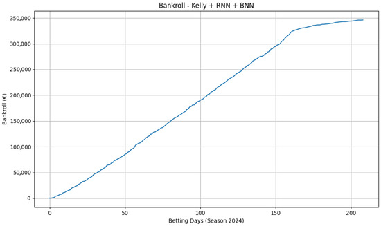
Figure 7.
Player-performance bankroll over the 2024 season using synthetic odds. Smoother growth suggests a denser set of positive-EV opportunities in thinner markets.
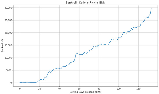
Figure 8.
Serie A moneyline bankroll (chronological evaluation, 0.3-Kelly, , stake cap EUR 100, start EUR 100). The upward drift with intermittent plateaus is consistent with selective wagering under the filter.
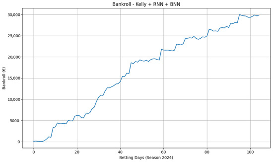
Figure 9.
Premier League moneyline bankroll (same protocol as Figure 8). The equity profile indicates stable edge with moderate drawdowns.
The histogram in Figure 10 illustrates the empirical distribution of bet sizes represented as fractions of the bankroll following the use of the 0.3 × Kelly multiplier. The density has a pronounced right skewness, with the bulk of bets concentrated within the range [0.03, 0.09] of total capital, and a minimal fraction surpassing 0.12.
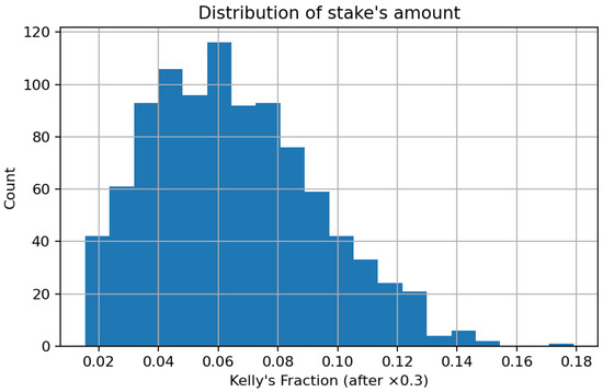
Figure 10.
Distribution of stake’s amount.
This trend illustrates that the implemented fractional-Kelly strategy effectively enforces risk discipline by allocating small chunks of money to the majority of positions while allowing for gradual increases in higher-confidence forecasts. The significant concentration in small fractions suggests a cautious exposure strategy that reduces the risk of catastrophic losses and fosters long-term capital preservation. From a portfolio-theoretic standpoint, the resultant stake distribution conforms to the notion of log-utility maximization under uncertainty, wherein growth is attained through numerous low-variance allocations rather than seldom substantial wagers. The histogram validates the internal consistency between the theoretical Kelly framework and its empirical application in this study, affirming that capital is allocated in proportion to anticipated informational advantage while preserving sensible leverage.
The scatter plot in Figure 11 illustrates the functional relationship between the staked capital fraction and the model-derived expected edge, denoted as
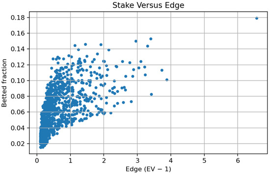
Figure 11.
Relationship between stake and expected edge.
A distinct positive monotonic correlation is evident: Greater estimated edges result in proportionately larger bet sizes, in accordance with the normative guidelines of the Kelly criterion. At near-zero or marginal thresholds, the allocation approaches minimal fractions (<0.04), demonstrating the self-regularizing nature of the technique in low-signal environments. Conversely, when the predicted value escalates, the staking function climbs gradually and asymptotically approaches its maximum limit of around 0.15–0.18, dictated by the fractional-Kelly coefficient. This relationship offers quantitative validation that the staking mechanism is consistently aligned with model-based probability evaluations, converting probabilistic advantages into capital exposure in a continuous and risk-conscious manner. The observed variability around the regression envelope indicates both market discretization in chances and the estimate noise intrinsic to probabilistic forecasts. The data substantiates the assertion that the adopted allocation policy maintains theoretical optimality while providing practical resilience against overconfidence and sampling variability.
The histogram in Figure 12 illustrates the empirical distribution of the model’s EV, calculated using Monte Carlo–Dropout probabilities.
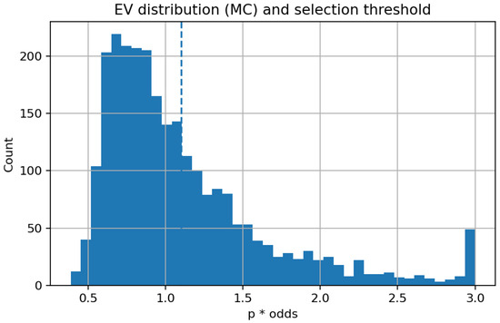
Figure 12.
Expected-value distribution and selection threshold.
The mass of the distribution is centred around one, indicating the efficacy of the betting market, where the majority of price–probability combinations produce an expected return near zero. The dashed vertical line indicates the operational threshold at EV = 1.10, which represents the lower limit for bet selection in the Kelly-based simulation. Observations over this threshold indicate instances where the model recognizes positive expected value prospects, factoring in market chances. The rapid decrease in frequency past the threshold signifies that such opportunities are statistically scarce, aligning with theoretical predictions for competitive marketplaces. The elongated right tail, despite its low population, underscores the existence of infrequent high-value forecasts that generate the majority of potential profit. This distribution thus offers empirical validation for the implemented EV filter, which adeptly balances coverage and quality by omitting the dense cluster of near-fair bets while preserving the limited collection of wagers with significant positive expectation.
The juxtaposition of market-implied probability and empirical outcome frequencies indicates a significant divergence from ideal calibration. In the majority of probability bins, the empirical win rate consistently falls short of the bookmaker-implied level, signifying a systematic overestimation of favourites and a commensurate underestimation of underdogs. This asymmetry indicates a continual behavioural and structural bias in betting markets, aligning with previous findings of risk-averse pricing and the influence of public mood. The existence of such miscalibration indicates that market odds do not serve as entirely effective estimators of actual outcome probabilities. Thus, a precisely defined predictive model possesses both theoretical and practical validity: It may yield unbiased probability estimates and enhance expected-value evaluation. The Bayesian recurrent neural architecture employed herein aims to accurately capture these deviations via calibrated probabilistic inference. In Figure 13, the disparity between suggested and empirical probability offers empirical support for model development, indicating that insights not entirely reflected in bookmaker odds can be derived from previous performance data. This statistic validates the primary assertion of the study, that machine learning-based probability modelling is a credible and potentially beneficial adjunct to market pricing processes.
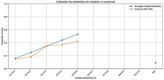
Figure 13.
Market-implied versus empirical calibration by probability bin.
For the logistic baseline, the merged dataset is partitioned into three non-overlapping subsets by season: (i) All seasons up to 2022 are used for training, (ii) season 2023 is reserved for model selection, and (iii) season 2024 is held out for final evaluation. The code enforces that date ranges do not overlap and that no game identifier appears in more than one split. To ensure that the logistic baseline has access exclusively to pre-game information, the feature vector excludes all post-game statistics. The only inputs retained are: (a) the home indicator, (b) market-implied probabilities (derived from published bookmaker odds), (c) closing spread and total, (d) the bookmaker overround, and (e) two past-only form features computed using a shifted rolling window (win rate and average points over the previous five games). Since these aggregates are computed with a one-step temporal shift, they incorporate only matches strictly preceding the game being predicted. Missing values are handled by an imputer fitted solely on the training data. On top of this pre-game feature set we train a family of logistic regression models with different regularisation strengths. Model selection is performed exclusively on the 2023 validation season using probabilistic metrics (log-loss and Brier score), not financial outcomes. The selected specification is the logistic model with , which achieves a validation log-loss of 0.6266. The frozen model is then applied to the 2024 test season, generating the probabilities used in the bankroll simulator under the same staking rules as in the main experiment. Under these strictly non-leaky conditions, the logistic baseline behaves as expected for a simple statistical model, with final bankroll, ROI, and hit rate as reported in Table 4. The main predictive architecture in the full experiment consumes a concatenation of: (i) the team and opponent box-score vector, (ii) the PCA-20 shot-location embedding, (iii) market-based features (implied probability, spread, total, overround), and (iv) short-term form indicators (rolling win rate, rolling points, home flag). In the no-leakage logistic baseline we restrict ourselves to the reduced, transparent subset listed above, which directly matches the feature engineering implemented in our public code. This explicit design makes it clear which sources of information enter the model, their dimensionality, the preprocessing steps applied, and the rationale for their inclusion.
Table 4.
Comparison between the market-implied and logistic-regression baselines under the same staking policy (fractional Kelly 0.3, EV , EUR 100 stake cap, odds cap = 10).
We also conduct an expanding-window, cross-season evaluation of the no-leakage logistic model to assess temporal robustness. For each test season from 2012 to 2024, all earlier seasons are used for training, the immediately preceding season is used for validation, and the current season is used exclusively for testing, thus preserving chronological order and preventing information leakage. As summarised in Table 5, the model exhibits stable probabilistic performance across seasons (mean accuracy , Brier score , log-loss , AUC ), and its betting performance remains close to break-even (mean final bankroll EUR 92.99, mean ROI with standard deviation ). This indicates that the behaviour observed on the 2024 test season is representative of the model’s typical out-of-sample performance rather than being driven by a single favourable split.
Table 5.
Cross-season robustness of the no-leakage logistic model over test seasons 2012–2024 using an expanding-window evaluation. Values are the mean and standard deviation across test seasons. BK denotes final bankroll under the Kelly-based staking rules (fractional Kelly , EV , EUR 100 starting bankroll, EUR 100 maximum stake, odds cap ).
The betting simulation is carried out under a set of idealised execution assumptions that follow common practice in the sports-analytics literature. In particular, we assume that all wagers are filled at the quoted decimal odds with no slippage, no liquidity constraints, and no partial execution, and that stakes can always be placed at the amounts dictated by the Kelly criterion (subject to the imposed cap). These conditions abstract away market frictions such as real-time price drift, bookmaker stake limits, and odds movement between bet identification and order placement. The simulation therefore represents an upper bound on achievable returns; its purpose is to provide a consistent and noise-free comparison between models under identical conditions. Relative differences between models are thus meaningful, whereas absolute profitability should be interpreted with caution.
To ensure that the model is not trivially reproducing bookmaker probabilities and to separate the contribution of different information sources, we conduct a structured ablation analysis (Table 6) isolating non-market features, market features, and their combination. The non-market model uses only team-level and performance-derived features (rolling indicators and contextual variables), achieving strong discriminative performance (AUC ) despite containing no market quantities. A market-only model is constructed in two forms: (i) an isotonic-regression calibration of the implied probabilities from closing moneylines, representing a best-possible probabilistic forecaster using only market information, and (ii) a logistic model trained exclusively on market features (spread, total, overround, and implied probability). Both market-only variants achieve reasonable calibration (Brier ) but substantially lower discrimination (AUC ) than the non-market model. When market information is added to the non-market feature set, the resulting fused model achieves the strongest overall performance (AUC , log-loss , Brier ). These results indicate that market and non-market information carry complementary predictive content, and that the fused model improves upon both components rather than collapsing to the bookmaker-implied probabilities. This substantially weakens any concern that the model’s performance is driven by trivial circularity between inputs and the odds used for value-based decision rules.
Table 6.
Ablation study comparing non-market, market-only, and fused models on the 2024 test set. The fused model integrates team- and performance-based features with market-derived information.
5. Discussion
The exploratory analysis confirms that the NBA environment over 2010–2024 is not stationary. Three-point volume roughly doubles (Figure 2), and average points per game increase in parallel (Figure 3). The rightward shift of the offensive rating density in 2024 relative to 2010 (Figure 4), together with a similar shift in defensive ratings (Figure 5), is consistent with higher pace and improved perimeter efficiency. In this context, per-100-possession standardisation and recent form windows (rolling last five games) are appropriate choices: They remove mechanical pace effects and allow the model to adapt to short-horizon changes in shot mix, tactical emphasis, and team health. The shot location embeddings likely contribute precisely because spatial tendencies (paint vs. perimeter, corner vs. above-the-break) evolved materially over the sample.
On NBA moneylines, the equity curve of the main uncertainty-aware win model (LSTM with MC-dropout) rises smoothly with intermittent plateaus and modest drawdowns (Figure 6). This pattern is consistent with calibrated sequential probabilities, filtered through the rule and fractional-Kelly staking, being converted into economic value. Two mechanisms plausibly contribute: (i) The recurrent input captures short-term momentum and roster shocks that are not always fully reflected in market prices; (ii) Monte Carlo dropout reduces overconfident selections, so fewer but higher-quality bets pass the decision threshold. Plateaus correspond to periods in which the uncertainty filter or the threshold suppress action (e.g., tighter pricing, larger vig), while shallow drawdowns reflect natural variance under a conservative 0.3-Kelly policy.
The scale of the final bankroll in moneyline simulations may appear surprisingly large relative to the EUR 100 starting capital and the EUR 100 per-bet cap. This outcome does not arise from unconstrained compounding, but from the interaction between the selection filter and odds structure. Since wagers are placed only when the expected value exceeds 1.1, the resulting portfolio is skewed toward higher-odds events, frequently in the 5.0–10.0 range. Even with a maximum stake of EUR 100, a single correct prediction in such conditions produces EUR 400–900 in profit, several times the return from a typical even-odds wager. Over more than one thousand bets with a hit rate near 60%, this concentration on infrequent but high-multiplier opportunities can plausibly compound into the observed capital growth. The figures therefore reflect selective wagering, calibrated probabilities, and high-odds pricing, rather than a relaxation of bankroll or staking constraints.
By contrast, the mixed or neutral results on spread and totals are consistent with those markets being more efficiently priced. Point spreads already encode a large fraction of team strength and situational information; the residual variance around the number is heavily influenced by noise (e.g., late-game fouling, end-game variance). Totals are additionally exposed to pace volatility and correlation structures (e.g., endgame possessions) that are difficult to forecast precisely from team-level aggregates alone. In such settings, the incremental predictive lift from the sequential model does not reliably exceed transaction costs and selection filters, so bankroll growth is flat to mildly negative.
Applying the same pipeline to football moneylines (Serie A and Premier League) yields upward-sloping equity curves with manageable drawdowns (Figure 8 and Figure 9). This suggests that the core ingredients—recent form sequences, opponent-adjusted features, and an uncertainty-aware decision rule—capture aspects of team strength that are not fully arbitraged even in mature markets. At the same time, the growth is stepwise rather than exponential, indicating that the selection filter is active (fewer but higher-edge opportunities) and that returns concentrate in specific subperiods (e.g., injury clusters, congested schedules).
The smoother growth observed with player-level classification under synthetic odds (Figure 7) points to richer, more idiosyncratic signal at finer granularity. Player performance is more volatile and information diffuses unevenly across sources, so a sequential model that conditions on recent usage and efficiency can identify edges more readily than at the team level. The main caveat is that pricing assumptions at player level are delicate; the results should therefore be interpreted as an illustration of how the pipeline behaves under alternative pricing regimes, not as direct evidence of real-world profitability. Nonetheless, they are coherent with the idea that thinner, less liquid markets may admit higher signal-to-noise ratios.
Across all bankroll figures, the decision layer shapes the trajectory as much as the classifier. Fractional-Kelly dampens volatility; the rule trades frequency for quality; and the per-bet cap limits extreme compounding. The resulting profiles—steady climbs punctuated by plateaus and shallow setbacks—are what one expects from a conservative staking policy applied to a model whose advantage is modest but persistent. Cross-market differences (moneyline vs. spreads/totals) manifest primarily as differences in slope (average edge) rather than as qualitatively different risk profiles, because the staking constraints are held fixed.
Figure 10, Figure 11, Figure 12 and Figure 13 provide additional insight into the internal dynamics of the decision pipeline. The histogram of stake fractions in Figure 10 confirms that the 0.3-Kelly policy enforces risk discipline: Most wagers concentrate on small slices of capital (typically within the first decile of the bankroll), with only a thin right tail. This shape is consistent with log-utility growth under uncertainty: many small exposures, occasional larger ones when the estimated edge is higher, and overall variance kept in check by the fractional multiplier and the per-bet cap.
Figure 11 shows the scatter plot of stake size against model-estimated edge, . As the edge increases, the stake fraction rises smoothly toward the ceiling induced by the fractional-Kelly coefficient and the stake cap. The visible dispersion around the trend line reflects both the discretisation of market odds and estimation noise in probabilistic forecasts, but the global pattern confirms that capital allocation is aligned with model confidence.
The expected-value distribution in Figure 12 is tightly massed around 1, illustrating that most price–probability pairs are close to fair and that markets are largely efficient. The operative threshold at deliberately trades frequency for quality: It removes the dense cluster of near-fair bets while preserving the sparse right tail of high-EV opportunities. This scarcity explains the stepwise equity profiles: plateaus when the filter suppresses action, punctuated by upward moves when rare, high-EV bets satisfy the selection rule.
Figure 13 compares market-implied and empirical calibration. The calibration curves display a systematic gap, with favourites tending to be overpriced (empirical win rates below implied) and underdogs underpriced. This structural miscalibration motivates a decision layer driven by calibrated model probabilities: When the model’s estimates exceed market-implied levels by a margin that survives the EV and Kelly filters, the pipeline identifies genuine value rather than amplifying noise. Taken together, Figure 10, Figure 11, Figure 12 and Figure 13 help explain why the moneyline (and synthetic player–prop) bankroll trajectories exhibit steady growth under the stated protocol, while spreads and totals remain neutral: Risk is mechanically constrained, and excess return arises primarily from rare high-EV opportunities associated with bookmaker miscalibration.
To clarify how classical probabilistic baselines use the available predictors, we computed SHAP values for the no-leakage logistic baseline on the 2024 test season, using the same chronological train–validation–test split and the pre-game feature set described in Section 4. The resulting global feature-importance ranking shows that the model relies predominantly on the market-implied probability for the team (mean ), with smaller contributions from recent form (rolling points: ; rolling win rate: ) and from pre-game betting information (total: ; overround: ). Home advantage () and spread () play only minor roles. The summary and bar plots in Figure 14 and Figure 15 show that the baseline behaves coherently with domain knowledge: Predictions are driven primarily by market expectations and simple form indicators, and no spurious or post-game features influence the output. This also explains why the logistic baseline, despite being well calibrated, fails to generate positive bankroll growth: It effectively reweights existing market information rather than uncovering independent signal.
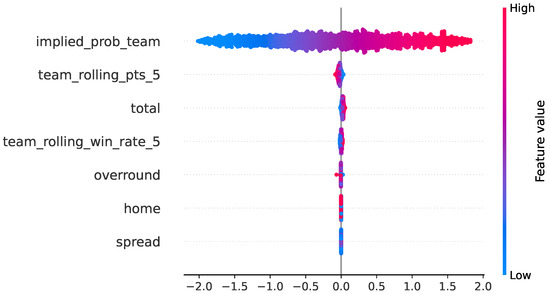
Figure 14.
SHAP summary (beeswarm) for the no-leakage logistic baseline on the 2024 test season.
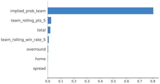
Figure 15.
Mean absolute SHAP values (global feature importance) for the no-leakage logistic baseline.
To assess whether the main conclusions depend on specific hyperparameter settings, we conducted a sensitivity and robustness analysis for the main moneyline model, covering decision thresholds, staking rules, temporal structure, and feature composition. The betting layer is evaluated over a grid of expected-value thresholds , Kelly multipliers , bet size caps EUR , and maximum odds filters . For each configuration we compute ROI, number of bets, and hit rate. The resulting surface is smooth across EV and Kelly parameters: Aggressive settings increase variance, but the model ranking and overall profitability pattern remain stable. Performance does not hinge on a narrow, finely tuned parameter choice.
We also vary the temporal window used to build past form features for the main model, testing sequences of lengths 3, 5, 7, and 10 games. Predictive metrics change gradually with sequence length, and the ranking of model variants is preserved. An ablation without shot-chart embeddings shows a consistent decrease in discrimination and calibration, confirming that spatial shooting patterns provide complementary information beyond team-level statistics.
Finally, a rolling cross-season evaluation of the no-leakage logistic baseline (Table 5) trains on seasons up to , validates on , and tests on t. Across test seasons 2012–2024, the logistic model achieves stable accuracy, Brier score, and log-loss, with mean AUC and betting performance clustered around break-even (mean final bankroll 92.99 EUR, mean ROI ). This confirms that the baseline’s behaviour on the 2024 test season is representative of its typical out-of-sample performance, and strengthens the comparison between the logistic baseline and the main uncertainty-aware pipeline.
Table 7 complements the bankroll analysis by reporting pure predictive and calibration metrics for the main baseline models on the 2024 test season. Logistic regression and XGBoost exhibit very similar behaviour: Both achieve accuracy around 0.68, Brier scores of about 0.20, and log-loss near 0.58, with AUC between 0.75 and 0.76 and low calibration errors (ECE , MCE ). The GRU sequence model is clearly inferior on all metrics, with higher Brier score and log-loss, lower AUC (0.65), and larger calibration errors. Overall, these results show that classical probabilistic baselines (logistic regression and boosted trees) are both competitive and well calibrated, while more complex sequence modelling does not automatically translate into better predictive or calibration performance. The added value of the proposed uncertainty-aware pipeline thus lies not in pointwise accuracy alone, but in its combination of calibrated probabilities, richer feature representations, and a disciplined decision layer that jointly drive long-run economic outcomes.
Table 7.
Test-set predictive performance (2024) with 95% bootstrap confidence intervals and calibration errors. ECE = expected calibration error; MCE = maximum calibration error.
6. Conclusions
The empirical analysis shows that an uncertainty-aware sequential pipeline can convert predictive lift into economic value, but only in markets where structural inefficiencies persist. On NBA moneylines, calibrated probabilities derived from the recurrent architecture, filtered through an criterion and disciplined by a fractional-Kelly staking rule, generate sustained and statistically coherent bankroll growth. This confirms that when model uncertainty is explicitly quantified and incorporated into the decision layer, predictive signals can be transformed into positive expected value. By contrast, the same pipeline applied to spreads and totals produces flat or mildly negative outcomes, consistent with these markets being more efficiently priced and leaving little exploitable residual structure. Player-level models, even when tested with synthetic odds, exhibit richer and more volatile signal in thinner markets, where informational asymmetries are slower to dissipate.
An important complementary result is that classical probabilistic baselines do not exhibit comparable behaviour. Market-implied probabilities remain at break-even under identical staking rules, logistic regression produces moderate predictive quality but negative financial returns, and boosted trees generate only modest gains. The exceptional growth observed in moneyline simulations therefore cannot be attributed to the staking mechanism, the evaluation protocol, or market prices alone: It emerges specifically from the interaction of the uncertainty-aware sequential predictor with a principled decision rule.
The diagnostic analyses clarify the mechanics behind this behaviour. The -Kelly rule tempers volatility; the threshold suppresses low-edge opportunities; and the 100 EUR stake cap prevents runaway compounding. Since the filter concentrates wagers on a sparse tail of high-odds, high-EV events, individual wins often produce large increments relative to the initial capital. Over more than a thousand chronologically ordered bets, this selective exposure plausibly accumulates into the observed growth without contradicting realistic risk constraints. The resulting equity curves—steady climbs interspersed with plateaus and shallow drawdowns—reflect precisely the dynamics expected from disciplined capital allocation under uncertainty.
The portability experiments reinforce these conclusions. Applying the same pipeline to Serie A and Premier League moneylines yields upward-sloping but less extreme trajectories, supporting the idea that the architecture extracts a transferable representation of team strength and short-term form. At the same time, the more moderate slopes outside the NBA underscore that profitability depends on the interplay between model skill and underlying market inefficiency.
Several limitations must be acknowledged. The simulations assume frictionless execution: All wagers clear at posted odds with no slippage, liquidity constraints, or bookmaker limits. The modelling pipeline excludes last-minute information such as injury news or real-time line movement, which materially affects real trading conditions. The historical coverage is restricted to the modern NBA era, and the shot chart embeddings rely on a specific CNN + PCA configuration together with Monte Carlo dropout for uncertainty. Moreover, bankroll growth remains sensitive to EV thresholds and Kelly fractions, and although robustness checks are provided, a full exploration of these hyperparameters is left for future work.
Future research should relax the idealised execution assumptions by introducing realistic liquidity and dynamic pricing. More expressive uncertainty-estimation methods (deep ensembles, Laplace approximations, SWAG) could be benchmarked against MC dropout. Extensions to incorporate player availability signals, rest patterns, and injury forecasts are natural next steps. Broader cross-league evaluations would improve ecological validity. Finally, integrating reinforcement learning decision layers or hierarchical Bayesian models for team and player strength may further clarify the boundaries of predictability in modern betting markets.
Author Contributions
Conceptualization, M.M.; methodology, M.M.; software, M.M.; validation, E.B. and A.G.; writing—original draft, M.M.; writing—review and editing, E.B. and A.G. All authors have read and agreed to the published version of the manuscript.
Funding
This research received no external funding.
Institutional Review Board Statement
Not applicable.
Informed Consent Statement
Not applicable.
Data Availability Statement
The data discussed in this paper are available at https://github.com/matteo6montrucchio/Dataset-Article.
Conflicts of Interest
The authors declare no conflicts of interest.
References
- Spherical Insights LLP. Global Online Sports Betting Market Size to Worth USD 162.92 Billion by 2033; CAGR of 11.15; Globe Newswire: New York, NY, USA, 2023. [Google Scholar]
- Baker, S.R.; Balthrop, J.; Johnson, M.J.; Kotter, J.D.; Pisciotta, K. Online Sports Betting Is Draining Household Savings; Kellog Insight: Evanston, IL, USA, 2024. [Google Scholar]
- Walsh, C.; Joshi, A. Machine learning for sports betting: Should model selection be based on accuracy or calibration? arXiv 2024, arXiv:2303.06021. [Google Scholar] [CrossRef]
- Zimmermann, A. Learning Predictive Models for Match Outcomes in US Sports, and Using Them to Bet. In Proceedings of the Sports Analytics: First International Conference, ISACE 2024, Paris, France, 12–13 July 2024; Springer: Berlin/Heidelberg, Germany, 2024; pp. 313–327. [Google Scholar] [CrossRef]
- Bunker, R.; Thabtah, F.A. A machine learning framework for sport result prediction. Appl. Comput. Inform. 2019, 15, 27–33. [Google Scholar] [CrossRef]
- Wang, J. Predictive Analysis of NBA Game Outcomes through Machine Learning. In Proceedings of the 6th International Conference on Machine Learning and Machine Intelligence (MLMI ’23), Chongqing, China, 27–29 October 2023; pp. 46–55. [Google Scholar] [CrossRef]
- Adam, C.; Pantatosakis, P.; Tsagris, M. On predicting an NBA game outcome from half-time statistics. Discov. Artif. Intell. 2024, 4, 111. [Google Scholar] [CrossRef]
- Hastie, T.; Tibshirani, R.; Friedman, J. The Elements of Statistical Learning: Data Mining, Inference and Prediction, 2nd ed.; Springer: Cham, Switzerland, 2009. [Google Scholar]
- Papadaki, I.; Tsagris, M. Are NBA Players’ Salaries in Accordance with Their Performance on Court? In Advances in Econometrics, Operational Research, Data Science and Actuarial Studies; Springer: Cham, Switzerland, 2022; pp. 405–428. [Google Scholar] [CrossRef]
- Krizhevsky, A.; Sutskever, I.; Hinton, G.E. ImageNet Classification with Deep Convolutional Neural Networks. Commun. ACM 2012, 60, 84–90. [Google Scholar] [CrossRef]
- Kandel, E.R. An introduction to the work of David Hubel and Torsten Wiesel. J. Physiol. 2009, 587, 2733–2741. [Google Scholar] [CrossRef] [PubMed]
- Zhang, X.; Zhang, X.; Wang, W. Convolutional neural network. In Intelligent Information Processing with Matlab; Springer: Cham, Switzerland, 2023; pp. 39–71. [Google Scholar]
- Jain, L.C.; Medsker, L.R. Recurrent Neural Networks: Design and Applications, 1st ed.; CRC Press, Inc.: Boca Raton, FL, USA, 1999. [Google Scholar]
- Rumelhart, D.E.; Hinton, G.E.; Williams, R.J. Learning Internal Representations by Error Propagation; MIT Press: Cambridge, MA, USA, 1985. [Google Scholar]
- Hochreiter, S.; Schmidhuber, J. Long Short-Term Memory. Neural Comput. 1997, 9, 1735–1780. [Google Scholar] [CrossRef] [PubMed]
- Strudel, R.; Pinel, R.G.; Laptev, I.; Schmid, C. Segmenter: Transformer for Semantic Segmentation. In Proceedings of the 2021 IEEE/CVF International Conference on Computer Vision (ICCV), Honolulu, HI, USA, 19–23 October 2025; pp. 7242–7252. [Google Scholar]
- Yang, J.; Li, C.; Zhang, P.; Dai, X.; Xiao, B.; Yuan, L.; Gao, J. Focal attention for long-range interactions in vision transformers. In Proceedings of the 35th International Conference on Neural Information Processing Systems (NIPS ’21), Red Hook, NY, USA, 6–14 December 2021. [Google Scholar]
- Zhou, T.; Wang, W.; Konukoglu, E.; Gool, L.V. Rethinking Semantic Segmentation: A Prototype View. arXiv 2022, arXiv:2203.15102. [Google Scholar] [CrossRef]
- Mikolov, T.; Joulin, A.; Chopra, S.; Mathieu, M.; Ranzato, M. Learning Longer Memory in Recurrent Neural Networks. arXiv 2015, arXiv:1412.7753. [Google Scholar] [CrossRef]
- John, L.; Kelly, J. A New Interpretation of Information Rate. Bell Syst. Tech. J. 1956, 35, 917–926. [Google Scholar] [CrossRef]


Disclaimer/Publisher’s Note: The statements, opinions and data contained in all publications are solely those of the individual author(s) and contributor(s) and not of MDPI and/or the editor(s). MDPI and/or the editor(s) disclaim responsibility for any injury to people or property resulting from any ideas, methods, instructions or products referred to in the content. |
© 2026 by the authors. Licensee MDPI, Basel, Switzerland. This article is an open access article distributed under the terms and conditions of the Creative Commons Attribution (CC BY) license.