Abstract
Mental disorders (MDs) constitute significant risk factors for self-harm and suicide. The incidence of MDs has been increasing annually, primarily due to inadequate diagnosis and intervention. Early identification and timely intervention can effectively slow the progression of MDs and enhance the quality of life. However, the high cost and complexity of in-hospital screening exacerbate the psychological burden on patients. Moreover, existing studies primarily focus on the identification of individual subcategories and lack attention to model explainability. These approaches fail to adequately address the complexity of clinical demands. Early screening of MDs using EEG signals and deep learning techniques has demonstrated simplicity and effectiveness. To this end, we constructed a Dual-Branch Network (DBN) leveraging resting-state Quantitative Electroencephalogram (QEEG) features. The DBN is designed to enable the detection of multiple categories of MDs. Firstly, a dual-branch feature extraction strategy was designed to capture multi-dimensional latent features. Further, we propose a Multi-Head Attention Mechanism (MHAM) that integrates dynamic routing. This architecture assigns greater weights to key elements and enhances information transmission efficiency. Finally, the diagnosis is derived from a fully connected layer. In addition, we incorporate SHAP analysis to facilitate feature attribution. This technique elucidates the contribution of significant features to MD detection and improves the transparency of model predictions. Experimental results demonstrate the effectiveness of DBN in detecting various MD categories. The performance of DBN surpasses that of traditional machine learning models. Ablation studies further validate the architectural soundness of DBN. The DBN effectively reduces screening complexity and demonstrates significant potential for clinical applications.
1. Introduction
Mental Disorders (MDs) refer to the collective term for various mental illnesses caused by disorders of brain functioning activity [1], which include Anxiety Disorder (AnxD), Obsessive–Compulsive Disorder (OCD), and Schizophrenia (SCZ), etc. MDs significantly impair of life and represent major risk factors for suicide and self-harm [2]. Stigmatization and impaired social functioning further exacerbate the condition. Due to disease-related stigma, self-denial, misdiagnosis, and underdiagnosis, many cases remain undetected and inadequately treated. Consequently, the prevalence of MDs continues to rise [3].
Early identification and timely intervention are highly effective in mitigating disease progression and improving prognosis [4]. However, in-hospital screening remains time-consuming, operationally cumbersome [5], and financially burdensome [6], making it difficult to expand coverage to high-risk populations. In addition, stigma and fear of stigmatization hinder patients’ willingness to seek medical care [7]. These challenges severely hinder the prevention and treatment of MDs. Therefore, enhancing the efficiency of the MD detection has become a pressing issue in addressing the global mental health crisis.
Developing deep neural networks (DNNs) based on electroencephalogram (EEG) signals can enhance detection efficiency and reduce screening costs. EEG provides feedback on the electrical activity and potential disorders of the human brain [8] and is the basis for MD screening. DNNs can effectively model the nonlinear features of EEG signals, providing reliable decision support [9]. Numerous studies have been conducted in this domain. Typical applications include studies on depressive disorder [10], SCZ [11], and post-traumatic stress disorder (PTSD) [12]. However, the large number of MD categories [1] poses challenges in adapting specific detection networks to diverse disorders. As a result, generalizing predictions across different MD categories remains difficult. Furthermore, the “black-box” nature of DNNs limits the explainability of results [13], hindering clinical acceptance.
In this paper, we propose a Dual-Branch Network (DBN). The DBN utilizes resting-state quantitative EEG (QEEG) features to detect multiple categories of MDs. Additionally, SHAP analysis based on cooperative game theory [14] is incorporated for feature attribution, enhancing the explainability of detection results. Our main contributions are summarized as follows:
- (1)
- A dual-branch feature extraction strategy is proposed to address the limitations of single-branch architectures, thereby providing more comprehensive feature representations for detection.
- (2)
- A Multi-Head Attention Mechanism (MHAM) with a dynamic routing is introduced to enhance attention to key elements and optimize feature space hierarchy, thereby improving information transmission efficiency.
- (3)
- SHAP analysis improves the explainability of DBN’s detections and increases the potential for clinical application.
2. Related Work
As stated earlier, neural networks offer a viable solution for the efficient and reliable detection of MD, which is an ongoing area of focus. Typical architectures include Multilayer Perceptron (MLP) and Convolutional Neural Networks (CNNs). Such models can automatically extract latent features from physiological signals and have thus received extensive attention.
The MLP is a classical classification model commonly used for the MD detection. Anxiety and depression are the most common diagnoses faced by the MLP. Bagheri et al. [15] developed an MLP to identify depression and anxiety in Iranian women with social dysfunction. It provided essential support for the development of targeted intervention initiatives. Mohamed et al. [16] conducted research on MDs in populations in conflict zones. This study utilized the MLP to detect different stages of anxiety and achieved favorable results. MLP’s salient issue is that determining the parameters requires multiple trials and errors, leading to the risk of overfitting. Therefore, the researchers attempted to improve the MLP performance through swarm intelligence algorithms. For instance, chicken swarm algorithms [17] and genetic algorithms [18] have optimized the parameter selection to upgrade accuracy while reducing overfitting. However, since the MLP is not sensitive to spatial or temporal structure, optimizing the parameter selection alone does not fundamentally break the performance bottleneck.
CNNs have become a popular choice for detecting MDs due to their superior performance in extracting local features. In Major Depressive Disorder (MDD) research, Uyulan et al. [19] processed EEG signals as grayscale images and used them to construct an adaptive learning model with a CNN architecture. The accuracy of the model was significantly improved compared to traditional approaches. Wang et al. [20] constructed a 3D Densely Connected CNN using magnetic resonance images of brain structures. It effectively extracted brain structural variability between MDD and healthy controls, with excellent performance. Besides MDD, CNNs are also common in Attention Deficit Hyperactivity Disorder (ADHD) screening. Wang et al. [21] constructed a CNN based on the independent components of functional MRI (fMRI) in individuals with ADHD. It effectively distinguished implicit feature variations and outperformed classical methods such as logistic regression and support vector machines. Akbugday et al. [22] proposed a CNN classifier for screening ADHD based on an EEG topographic feature map, which outperformed machine learning models. Furthermore, CNNs also shone in detecting PTSD [23], sleep disorders [24], and psychological disorders [25]. The CNN has powerful feature modeling capabilities. However, it is less efficient in processing tabular features, with a risk of losing global information.
The emergence of novel neural networks also provides ideas for designing the detection architectures for MD. The MHAM and the derived Transformer [26] are typical cases. Xia et al. [27] combined the MHAM and the CNN to achieve the MDD classification by EEG. The MHAM learned the latent connectivity relationships of EEG channels. Then, features were extracted by the CNN and fed into the fully connected layer for detection. The study achieved an average accuracy of 91.06%, which was superior to the comparison methods. In addition, Transformer, which focuses on the MHAM, has also received attention from many scholars for its excellent feature modeling performance. Aina et al. [28] designed an integrated learning architecture that incorporates the CNN and Visual Transformers. It achieved the prediction of depression, anxiety, etc., from the facial emotion recognition dataset with an accuracy of 81%. The spotlight was on Aina’s attention to explainability, with contributing areas of decision support highlighted in the image. The MHAM is effective in reducing redundancy but is under-examined in modeling hierarchical relationships of critical features to improve the efficiency of information transmission.
Current research in MD detection focuses on analyzing brain physiological signals, commonly fMRI and EEG. We chose EEG because it is cheap and easy to obtain, which reduces the cost of patient screening. In addition, the MD screening process has become streamlined. In constructing models, most existing methods rely on single-channel extraction of features to detect an individual category of the MD. Inadequate learning of features is a shortcoming. Meanwhile, clinical practice frequently faces more complex disease conditions and co-morbidities [29,30]. Therefore, the model’s effectiveness in detecting different MDs is unknown, making it difficult to migrate the application immediately. In addition, clinical requires a high degree of transparency in the detection results. However, most researchers tend to emphasize accuracy improvement and pay insufficient attention to explainability. Therefore, we construct the DBN using QEEG features to improve the detection accuracy and explainability for MDs.
3. Methods
3.1. The DBN Overall Architecture
The DBN primarily consists of two parts: a dual-branch feature extraction strategy and the MHAM with a dynamic routing, as illustrated in Figure 1. In the dual-branch feature extraction strategy, the MLP and the 1D-CNN model the global complex nonlinear relationships and local features of QEEG features. We use the power spectral density (PSD) and coherence value of each band of the QEEG signal to detect the MD. There is an interaction between these features of sensory signals at different locations, i.e., implicit spatiotemporal relations. 1D-CNN models local features of such relations. In addition, we introduce MLP modeling the global relation, considering the tabular property of QEEG features. The two feature extractors complement each other to provide more comprehensive information for MD detection.
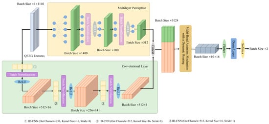
Figure 1.
Overall architecture design of the DBN.
Fusion of two-branch outputs yields computed results. Further, DBN incorporates the MHAM with dynamic routing. The MHAM runs multiple independent attentional mechanisms in parallel to highlight key information, thus obtaining the attentional distribution in different subspaces of the input sequence. Then, the dynamic routing optimizes the spatial hierarchy of attentional features to ensure efficient information delivery. The fully connected layer adapts the output dimension of the dynamic routing. Finally, the detection result of the MD is obtained by computation. The following subsections provide a detailed description of the key components of the DBN.
3.2. Dual-Branch Feature Extraction Strategy
As in Figure 1, the inputs are extracted by the MLP and the 1D-CNN for global nonlinear relationships and local features, respectively, to achieve feature modeling. Denote raw QEEG features as , , , where is the feature dimension and is the batch size. The MLP branch output is given by the following equation:
where , is the MLP weight parameter for each layer, is the bias term. denotes the batch normalization and GELU activation operations performed on the hidden layer output, computed as
where denotes a back-to-front series calculation operation.
In the 1D-CNN branch, the raw feature is convolved in 3 layers to get the output , computed as
where , , denotes performing convolution, batch normalization, and ReLU activation on the input, computed as
The layer convolution output is:
where is the number of convolution kernels in layer . denotes the result of convolving the input with the convolution kernel in layer , , , , and is the output vector dimension.
is fed into batch normalization and ReLU activation to obtain the output, and multilayer concatenation operations to obtain the output of the convolutional branch . The dual-branch feature extraction strategy output is obtained by concatenating the MLP output and the 1D-CNN output , as shown in Equation (6).
3.3. The MHAM with a Dynamic Routing
The MHAM enhances the weighting of the core elements in . On this basis, the dynamic routing of capsule neural networks [31] is integrated to combine and optimize the feature space hierarchy. is linearly transformed to obtain the query vector , the key vector , and the value vector . Denote , , is the output dimension of the dual-branch feature extraction strategy, then we have
where , is the linear layer weight matrix.
We determine the number of attention heads in the MHAM according to the following:
- Refer to the criterion for the value of in [26].
- Consider the dimension matching constraint with .
- The computational overhead associated with increasing is non-negligible.
- Combine the research needs and pre-experiments to give the final value.
According to , , , and can be grouped into , where , is the vector dimension corresponding to each head. , and . Each head output can be obtained from Scaled Dot-Product Attention [26]:
where is the output of the head. The output of the MHAM is obtained by concatenating the output of each head and performing a linear transformation, computed as
where , is the weight matrix of the linear layer.
In the dynamic routing, is computed as a prediction vector from the transformation matrix , is the product of the number and the dimension of the output vectors.
The output of the dynamic routing can be calculated from the according to Equation (11).
where is the coupling coefficient, which can be calculated from Equation (12).
where is the number of output vectors, is the routing weight. The loop iterates to update the routing weights . Further, the coupling coefficients and the output are updated according to Equations (11) and (12). The dynamic routing output is obtained by reaching the specified number of iterations. The batch output of the dynamic routing is . Input the flattened into the fully connected networks for dimensional matching. Finally, calculation is performed to obtain the detection results, as shown in Equation (13).
The cross-entropy loss function is chosen to measure the deviation of the predicted value from the target value when the error is back-propagated by
where is the true label of sample. After obtaining the loss from Equation (14), the parameters of the DBN are iteratively updated according to the back propagation principle to complete the training process.
3.4. Explainability of the DBN: SHAP Analysis
SHAP analysis allows a quantitative explanation of detection results and improves the transparency of the DBN. The core is the Shapley value calculation to measure the marginal contribution of different features to the outcome. Denote the set of raw features as , where , is the total number of features and is the number of samples, then the Shapley value of feature is:
where is the subset of various features that do not contain feature . is the subset containing the feature . is the corresponding detection result for the subset containing feature . is the corresponding detection result for the subset that do not contain feature .
According to Equation (15), indicates the relative importance of QEEG features on MDs detection results. The higher is, the greater the contribution of feature to MDs detection. Since the DBN is a kind of DNN, we choose the GradientExplainer to complete the feature importance assessment and the Shapley value dependency calculation.
4. Dataset and Experimental Settings
4.1. Dataset Introduction
The dataset was provided by [32], approved by the ethical review board (20-2019-16), and made publicly available. It was obtained from the Resting State Assessment Study at SMG-SNU Boramae Medical Center, South Korea, from January 2011 to December 2018. The initial diagnosis was made by a psychiatrist based on DSM-IV criteria promulgated by the American Psychiatric Association (APA) [33]. Clinical confirmation of diagnostic findings was completed by two psychiatrists and two psychologists in 2019.
The dataset consists of 945 subjects’ medical records, psychologically assessed IQ scores, and QEEG features from resting-state assessments. A total of 850 patients with MDs and 95 healthy controls are included. The inclusion criteria are as follows: age between 18 and 70 years old; fulfillment of the diagnosis shown in Table 1; and no difficulty in reading, hearing, writing, or understanding the Korean language. The exclusion criteria are as follows: lifetime and current medical history of neurologic disease or brain injury, neurodevelopmental disorders (i.e., intellectual disability with IQ < 70 or borderline intellectual functioning (70 < IQ < 80), tic disorders, ADHD), or any neurocognitive disorder. Our research focuses on six main categories and nine subcategories underneath, as detailed in Table 1. Among them, the OCD and the SCZ are not further subdivided.

Table 1.
Description of the composition of the experimental dataset.
The detailed processing flow and equipment used for QEEG acquisition are recorded in [32]. We visualize it in Figure 2 to enhance understanding. QEEG is 19 channels of data collected during the 5 min closed-eye resting state. Channels and sensor locations are identified according to the 10–20 international standard lead system. Among them, the acquisition channels include Fp1, Fp2, F7, F3, Fz, F4, F8, T7, C3, Cz, C4, T8, P7, P3, Pz, P4, P8, O1, and O2, and the sensor locations are marked in Figure 3. The QEEG is converted into a combination of the PSD and functional connectivity (FC) in six frequency bands: delta (1–4 Hz), theta (4–8 Hz), alpha (8–12 Hz), beta (12–25 Hz), high beta (25–30 Hz), and gamma (30–40 Hz). The FC is represented by the coherence value. Figure 3 shows the visualization of the mean values of the PSD of MNE-Python [34] for each band of the six categories of MDs. The dimension of the processed QEEG features is 1140, including power spectral density () and FC (). We use QEEG features for our study and divide it into an 8:2 ratio between the training and testing sets.
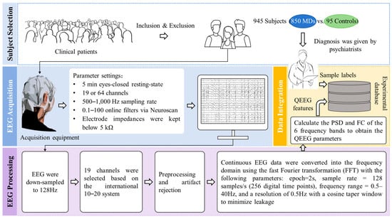
Figure 2.
Introduction to the dataset preprocessing process.

Figure 3.
Mean value of power spectral density in each frequency band.
4.2. Experimental Settings
The experimental simulation environment is built based on Windows 11 and the PyTorch deep learning framework. Acceleration of the training process is performed using a GPU, corresponding to CUDA version 12.0. The programming language is Python, version 3.8.0, and Torch version 1.12.0. The cross-entropy loss function and the Adam optimizer are chosen for the experiment. The maximum number of iterations is 500, and the minimum number of iterations is 20. The early stopping strategy is used to improve the overfitting problem that may occur during model training. Details of the experimental parameter configurations are shown in Table 2.
Table 2.
Details of experimental settings.
4.3. Performance Evaluation Metrics
Clinical diagnosis has a high cost associated with detection errors across various categories, and all samples require equal treatment. Hence, we use the macro-averaged metrics as the performance evaluation term. To evaluate the performance of the DBN, we choose the confusion matrix, Accuracy (), macro average F1 score (), and ROC curve as evaluation metrics, as stated below:
Confusion matrix: It describes the correspondence between the predicted and true values for the MDs/healthy subjects in matrix form.
: It describes the percentage of correctly identified MDs and healthy subjects out of all samples detected. It is calculated as follows:
: It is the harmonic mean of macro average Precision () and macro average Recall (). denotes the mean of percentages of two categories in the sample predicted to be MDs/healthy that are truly MDs/healthy. denotes the mean of percentages of two categories, where the true value is MDs/healthy and the prediction is also MDs/healthy.
is calculated as follows:
ROC curve: It reflects the effectiveness of the DBN detection through the trend of correlation between False Positive Rate () and True Positive Rate (). The effectiveness of MD detection can be directly observed by the area between the curve and the abscissa (AUC value).
In Equations (16) and (17), indicates the number of samples in which patients with real MDs are predicted to be ill, describes the number of healthy subjects detected to have MDs, is the number of healthy subjects detected to be healthy, and denotes the number of MD subjects predicted to be healthy.
5. Results and Discussion
5.1. Effectiveness of the DBN in the Detection of MDs
We disassembled the detection of MDs into the binary classification task and evaluated the performance on the test set. Figure 4 shows the confusion matrix of the detection results for the six main MDs. Detection results for the nine subcategories are given in Figure 5. The horizontal coordinate of the confusion matrix is the predicted prevalence, and the vertical coordinate is the true clinical diagnosis. The darker the color, the greater the number of subjects.
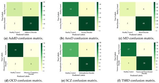
Figure 4.
Detection results of the six main MDs.
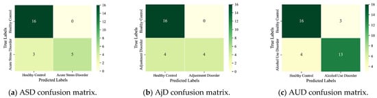
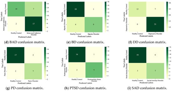
Figure 5.
Detection results for the nine subcategories.
As seen, the six main MDs are recognized correctly as AddD (95%), AnxD (81%), MD (91%), OCD (75%), SCZ (87%), and TSRD (87%). The recognition rates for the nine subcategories are as follows: ASD (63%), AjD (50%), AUD (76%), BAD (89%), BD (69%), DD (84%), PD (78%), PTSD (82%), and SAD (70%). The results show that the DBN can fulfill the task of detecting different categories of MDs. In parallel, we also note that the ASD and the AjD have lower recognition accuracies. The reason is that the DBN does not learn enough features for small sample objects. Improvement is expected through sample enhancement.
From the experimental results, the DBN is adaptable to screening for multiple categories of MDs, which is consistent with clinical practice. The DBN provides important support for the adjunctive diagnosis of clinically complex diseases or comorbid conditions.
5.2. Ablation Experiments: Structural Validity Analysis
To verify the validity of the DBN structure, we disassembled the model and completed the analysis of the ablation experiment. We evaluated the DBN performance in terms of and , and the results are shown in Table 3 and Table 4. We masked the network structure to evaluate the effectiveness of the dual-branch feature extraction strategy and the dynamic routing.
Table 3.
Detection results of the six main MDs.
Table 4.
Detection results of the nine subcategories.
Firstly, we removed the MLP and the 1D-CNN in the dual-branch feature extraction strategy, respectively. Among the six categories of results, and for dual-branch feature extraction strategies outperform the MLP in four categories, as well as outperform 1D-CNN in five categories. The detection results of the refined nine MDs also show the effectiveness of the dual-branch feature extraction strategy. It outperforms the MLP in both and in seven detections. Meanwhile, it leads the performance in six detection tasks compared to the 1D-CNN.
In addition, we also analyzed the structural validity of the MHAM with a dynamic routing. The analysis reveals that the dynamic routing performs optimally for the six main categories of MDs. Among them, the and of the detection results of the OCD are the most significantly improved, with 11% and 12%, respectively. The AnxD’s detection improves by 5% and 7%, and the SCZ improves by 2%. The performance of the remaining three categories is flat. In most of the nine subcategory experiments, detection is improved. We also note that DD detection is ineffective. By calculating the evaluation metrics, we found that the DBN is poor at recognizing the HC in this experiment. This is due to the unbalanced sample shares of the two categories, which require data governance.
The ablation experiments show that the dual-branch feature extraction strategy can mine global complex nonlinear relationships and local features in QEEG features. This provides a rich and reliable verdict for the detection of MDs. And the MHAM with dynamic routing can effectively combine and deliver key information to support the detection of MDs.
5.3. Comparative Experiment: Performance Advanced Level Analysis
We designed a 5-fold cross-validation experiment to verify the state-of-the-art of model performance. In experiments, we compared the DBN with commonly used machine learning models for MDs prediction (e.g., SVM [35], Random Forest [36], XGBoost [37], and LightGBM [38]). The performance comparison results are presented in the form of ROC curves, which are detailed in Figure 6 and Figure 7. We recorded the , , and AUC value for each fold and averaged them to obtain the final results. The subplots in Figure 6 and Figure 7 show the results of the binary classification for different MDs and healthy controls.
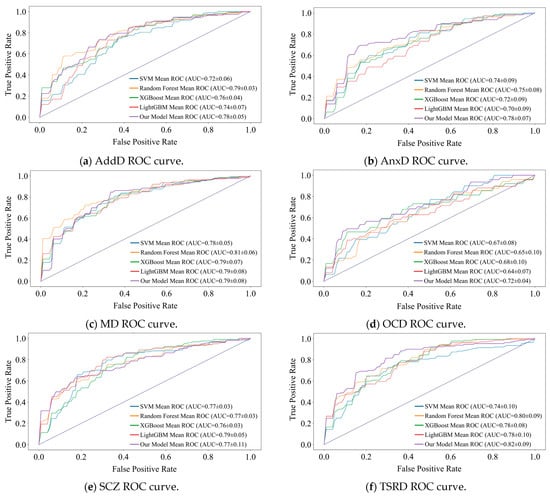
Figure 6.
Comparison of recognition performance of the six main MDs.
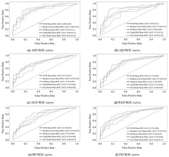
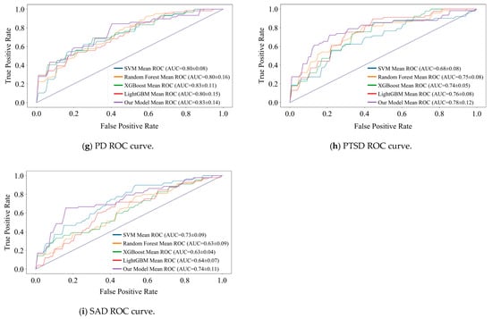
Figure 7.
Comparison of recognition performance of the nine subcategories.
AUC value is our main observation. As can be seen in Figure 6, the DBN improves over the optimal model by 3%, 4%, and 2% for the three detection tasks of AnxD, OCD, and TSRD. The other three tasks perform similarly to the optimal model. Of the nine subcategories, seven perform optimally and two perform similarly. It demonstrates that the DBN is more adaptable to new samples than machine learning.
The shape of the ROC curve is also an important indicator of performance. It is observable that the ROC curve of DBN tends to be steeper in the early stages in most tasks, especially in the detection of nine categories. It indicates that the DBN maintains a high even at a lower , and shows its strong discrimination ability for different categories. In addition, there are intersections between the ROC curves of various models. Therefore, there is no “absolute advantage”, which places demands on the adaptability of the model. DBN outperforms the comparison model at low , and is suitable for medical diagnosis scenarios with low tolerance for false positives.
The lack of data significantly affects all models. As the result shows, the ROC curves of all models exhibit sawtooth fluctuations rather than smooth curves. The reason for this phenomenon is that we split the raw dataset, resulting in a limited sample size. Under a limited test set, changes in the threshold have a discrete effect on and , resulting in a sawtooth-shaped ROC curve. Despite this issue, the overall trend of the average ROC curve and its AUC value remains a reliable indicator for evaluating performance.
Cross-validation results show that machine learning models perform very differently in detecting multiple subcategories of MDs. And the DBN can be adapted to the detection scenarios of the multiple subcategories and outperforms machine learning models for tabular data detection. The DBN exhibits robust prediction for the multiple categories of MDs and generalization for the emergence of new cases.
5.4. SHAP Analysis
Feature attribution analysis can effectively enhance the explainability of the DBN detection results, which is important for clinical applications. We implemented the DBN explainability research using SHAP analysis, as shown in Figure 8 and Figure 9. A summary of the contribution of different QEEG features to the detection of MDs is shown in two groups of bee colony plots.
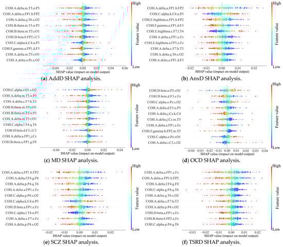
Figure 8.
Bee colony diagrams of SHAP analysis of the six main categories.
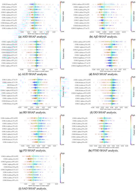
Figure 9.
Bee colony diagrams of SHAP analysis of the nine subcategories.
In the bee colony plot, the horizontal coordinates indicate the Shapley values of QEEG features, reflecting their impact on detection results. The left-hand side gives a ranking of important features based on the mean absolute Shapley value. Points in the diagram are raw values of features, with different values indicated by color differences. The further to the right the point is, the greater the positive effect on the output; conversely, the more negative the effect.
The results show that the main influencing factors are coherence values, e.g., COH.A.delta.a.FP1.b.FP2 and COH.C.alpha.r.O1.s.O2. It indicates that the synergistic effect of neural activity in different brain regions has a significant impact on the detection of MDs. Therein, COH.A.delta.a.FP1.b.FP2 has significant effects on the detection of the two main categories and five subcategories. Suggests that prefrontal brain functional connectivity provides support for the detection of a variety of MDs. This finding is supported by previous research [39]. Researchers concluded that prefrontal EEG is closely related to MDs and used a 3-electrode (Fp1, Fpz, and Fp2) to obtain signals to detect major depression.
Therefore, the SHAP is effective in providing a reliable explanation for the attribution analysis of the DBN detection results. It reveals the dependence of the pathogenesis of multiple MDs on functional brain connectivity. Thus, it enhances the transparency and reliability of the predictive results of the DBN. Our model provides novel ideas for intelligent clinical decision support.
Although the DBN improves the efficiency and explainability of MD detection, it has limitations. On the one hand, the size of the dataset is limited. The raw dataset contains only 945 samples, and the sample splitting for the binary classification further reduces the data size. The lack of samples leads to unstable training and uneven detection in machine learning, as shown in Section 5.3. Despite the improved detection quality, the small sample size still leads to insufficient feature learning by the DBN. For example, it detects ASD and AjD with low rates of correctness (Section 5.1) and does not discriminate sufficiently between DD and HC (Section 5.2). On the other hand, we split the detection into a binary classification problem, which also increases the workload. However, the problems are not insurmountable. The gradual improvement of medical data sharing policies and the development of wearable smart detection devices will solve the data limitation. In addition, multi-category detection for MDs supported by massive data will also be developed. Despite the limitations, there is reason to believe that DNNs have a promising future for clinical applications in MDs’ detection based on the DBN performance.
6. Conclusions
We propose the DBN for enhancing the quality of detecting multiple MDs with QEEG features. The DBN is evaluated in terms of detection accuracy, structural validity, performance advances, and explainability. According to the results, the DBN can accurately detect most categories of MDs, and it outperforms the machine learning models. The ablation analysis demonstrates the effectiveness of the dual-branch feature extraction strategy and the MHAM with dynamic routing. Additionally, SHAP analysis enhances the explainability of the DBN detection results by visualizing the influence of QEEG features. Overall, the DBN improves the detection efficiency of MDs with computer-aided technology. Moreover, relying only on EEG signals as the basis for judgment simplifies the clinical screening process and reduces the financial burden on patients.
Our work also has limitations, and the limited data resources affect the DBN performance improvement. In subsequent work, we will attempt to integrate medical data resources and introduce sample enhancement to improve the quality of MDs’ detection. Moreover, although our work demonstrates the excellent performance of the DBN through k-fold cross-validation (k = 5), the impact of different random initializations on the results is not systematically evaluated. Therefore, in our following work, we will further validate the robustness of the model by conducting large-scale multi-randomized seed experiments.
Author Contributions
All authors, L.Z., H.C. and Y.P., contributed to different aspects of this work. L.Z. and H.C. were responsible for conceptualization, data collection, software implementation, and experimental validation. L.Z. also led the original draft preparation and manuscript revision. H.C. contributed to the formal analysis and manuscript review. Y.P. contributed to data analysis and model construction, and provided ongoing guidance throughout the research process. All authors have read and agreed to the published version of the manuscript.
Funding
This research received no external funding.
Institutional Review Board Statement
Not applicable.
Informed Consent Statement
Not applicable.
Data Availability Statement
The original dataset presented in this study can be found in online repositories at https://osf.io/8bsvr/ (accessed on 24 December 2024). If there are difficulties accessing the website, the alternative URL is https://www.kaggle.com/datasets/shashwatwork/eeg-psychiatric-disorders-dataset (accessed on 24 December 2024). The code is open source at https://github.com/longhao-zhang-ustb/DBN_MODEL (accessed on 30 August 2025). Further inquiries can be directed to the corresponding author.
Conflicts of Interest
The authors declare no conflicts of interest.
Abbreviations
The following abbreviations are used in this manuscript:
| DBN | Dual-Branch Network |
| MDs | Mental Disorders |
| EEG | Electroencephalogram |
| QEEG | Quantitative Electroencephalogram |
| SHAP | Shapley Additive exPlanations |
| AnxD | Anxiety Disorder |
| OCD | Obsessive–Compulsive Disorder |
| SCZ | Schizophrenia |
| DNNs | Deep Neural Networks |
| PTSD | Post-Traumatic Stress Disorder |
| MHAM | Multi-Head Attention Mechanism |
| MLP | Multilayer Perceptron |
| CNNs | Convolutional Neural Networks |
| MDD | Major Depressive Disorder |
| ADHD | Attention Deficit Hyperactivity Disorder |
| fMRI | functional FMRI |
| APA | American Psychiatric Association |
| AddD | Addictive Disorder |
| AUD | Alcohol Use Disorder |
| BAD | Behavioral Addiction Disorder |
| PD | Panic Disorder |
| SAD | Social Anxiety Disorder |
| HC | Healthy Control |
| MD | Mood Disorder |
| BD | Bipolar Disorder |
| DD | Depressive Disorder |
| TSRD | Trauma- and Stress-Related Disorder |
| ASD | Acute Stress Disorder |
| AjD | Adjustment Disorder |
| PSD | Power Spectral Density |
| FC | Functional Connectivity |
References
- Broyd, S.J.; Demanuele, C.; Debener, S.; Helps, S.K.; James, C.J.; Sonuga-Barke, E.J. Default-mode brain dysfunction in mental disorders: A systematic review. Neurosci. Biobehav. Rev. 2009, 33, 279–296. [Google Scholar] [CrossRef]
- Brausch, A.M.; Whitfield, M.; Clapham, R.B. Comparisons of mental health symptoms, treatment access, and self-harm behaviors in rural adolescents before and during the COVID-19 pandemic. Eur. Child Adolesc. Psychiatry 2023, 32, 1051–1060. [Google Scholar] [CrossRef]
- World Health Organization. World Mental Health Report: Transforming Mental Health for All; World Health Organization: Geneva, Switzerland, 2022. [Google Scholar]
- Reynolds, C.F., 3rd; Jeste, D.V.; Sachdev, P.S.; Blazer, D.G. Mental health care for older adults: Recent advances and new directions in clinical practice and research. World Psychiatry 2022, 21, 336–363. [Google Scholar] [CrossRef]
- Bass, V.; Brown, F.; Beiser, D.G.; Peterson, T.; Gibbons, R.D.; Nagele, P. Preoperative assessment of anxiety and depression using computerized adaptive screening tools: A pilot prospective cohort study. Anesth. Analg. 2022, 134, 853–857. [Google Scholar] [CrossRef]
- Arias, D.; Saxena, S.; Verguet, S. Quantifying the global burden of mental disorders and their economic value. eClinicalMedicine 2022, 54, 101675. [Google Scholar] [CrossRef]
- Li, L.; Peng, W.; Rheu, M.M.J. Factors predicting intentions of adoption and continued use of artificial intelligence chatbots for mental health: Examining the role of UTAUT model, stigma, privacy concerns, and artificial intelligence hesitancy. Telemed. e-Health 2024, 30, 722–730. [Google Scholar] [CrossRef] [PubMed]
- Kopanska, M.; Ochojska, D.; Trojniak, J.; Sarzynska, I.; Szczygielski, J. The role of quantitative electroencephalography in diagnostic workup of mental disorders. J. Physiol. Pharmacol. 2024, 75, 39415522. [Google Scholar]
- Sharma, C.M.; Chariar, V.M. Diagnosis of mental disorders using machine learning: Literature review and bibliometric mapping from 2012 to 2023. Heliyon 2024, 10, e32548. [Google Scholar] [CrossRef] [PubMed]
- Khan, S.; Umar Saeed, S.M.; Frnda, J.; Arsalan, A.; Amin, R.; Gantassi, R.; Noorani, S.H.; Nisar, H. A machine learning based depression screening framework using temporal domain features of the electroencephalography signals. PLoS ONE 2024, 19, e0299127. [Google Scholar] [CrossRef]
- Alazzawı, A.; Aljumaili, S.; Duru, A.D.; Uçan, O.N.; Bayat, O.; Coelho, P.J.; Pires, I.M. Schizophrenia diagnosis based on diverse epoch size resting-state EEG using machine learning. PeerJ Comput. Sci. 2024, 10, e2170. [Google Scholar] [CrossRef]
- Yamunarani, T.; Zaki, W.S.B.W.; Elango, S.; Chandrasekaran, G.; Yamuna, S.; Kumar, K.K.; Maheswaran, S. Analysis of Post-Traumatic Stress Disorder (PTSD) Using Electroencephalography. In Proceedings of the 2024 15th International Conference on Computing Communication and Networking Technologies (ICCCNT), Kamand, India, 24–28 June 2024; IEEE: Piscataway, NJ, USA, 2024; pp. 1–6. [Google Scholar]
- Huang, S.-M.; Wu, F.-H.; Ma, K.-J.; Wang, J.-Y. Individual and integrated indexes of inflammation predicting the risks of mental disorders-statistical analysis and artificial neural network. BMC Psychiatry 2025, 25, 226. [Google Scholar] [CrossRef]
- Lundberg, S.M.; Lee, S.I. A unified approach to interpreting model predictions. Adv. Neural Inf. Process. Syst. 2017, 30, 4768–4777. [Google Scholar]
- Bagheri, S.; Taridashti, S.; Farahani, H.; Watson, P.; Rezvani, E. Multilayer perceptron modeling for social dysfunction prediction based on general health factors in an Iranian women sample. Front. Psychiatry 2023, 14, 1283095. [Google Scholar] [CrossRef]
- Mohamed, E.S.; Naqishbandi, T.A.; Bukhari, S.A.C.; Rauf, I.; Sawrikar, V.; Hussain, A. A hybrid mental health prediction model using Support Vector Machine, Multilayer Perceptron, and Random Forest algorithms. Healthc. Anal. 2023, 3, 100185. [Google Scholar] [CrossRef]
- Saranya, S.; Kavitha, N. Robust feature selection with chicken swarm intelligence improved multilayer perceptron for early detection of mental illness disorder. J. Theor. Appl. Inf. Technol. 2022, 100, 3337–3345. [Google Scholar]
- Oweimieotu, A.E.; Akazue, M.I.; Edje, A.E. Designing a Hybrid Genetic Algorithm Trained Feedforward Neural Network for Mental Health Disorder Detection. Adv. Multidiscip. Sci. Res. J. Publ. 2024, 12, 49–62. [Google Scholar] [CrossRef]
- Uyulan, C.; Ergüzel, T.T.; Unubol, H.; Cebi, M.; Sayar, G.H.; Asad, M.N.; Tarhan, N. Major depressive disorder classification based on different convolutional neural network models: Deep learning approach. Clin. EEG Neurosci. 2021, 52, 38–51. [Google Scholar] [CrossRef]
- Wang, Y.; Gong, N.; Fu, C. Major depression disorder diagnosis and analysis based on structural magnetic resonance imaging and deep learning. J. Integr. Neurosci. 2021, 20, 977–984. [Google Scholar] [CrossRef]
- Wang, D.; Hong, D.; Wu, Q. Attention deficit hyperactivity disorder classification based on deep learning. IEEE/ACM Trans. Comput. Biol. Bioinform. 2022, 20, 1581–1586. [Google Scholar] [CrossRef]
- Akbugday, B.; Bozbas, O.A.; Cura, O.K.; Pehlivan, S.; Akan, A. Detection of Attention Deficit Hyperactivity Disorder by Using EEG Feature Maps and Deep Learning. In Proceedings of the 2023 31st European Signal Processing Conference (EUSIPCO), Helsinki, Finland, 4–8 September 2023; IEEE: Piscataway, NJ, USA, 2023; pp. 1105–1109. [Google Scholar]
- Ismail, N.H.; Liu, N.; Du, M.; He, Z.; Hu, X. A deep learning approach for identifying cancer survivors living with post-traumatic stress disorder on Twitter. BMC Med. Inform. Decis. Mak. 2020, 20, 1–11. [Google Scholar] [CrossRef] [PubMed]
- Phan, D.V.; Yang, N.P.; Kuo, C.Y.; Chan, C.-L. Deep learning approaches for sleep disorder prediction in an asthma cohort. J. Asthma 2021, 58, 903–911. [Google Scholar] [CrossRef]
- Huang, P. A mental disorder prediction model with the ability of deep information expression using convolution neural networks technology. Sci. Program. 2022, 2022, 4664102. [Google Scholar] [CrossRef]
- Vaswani, A. Attention is all you need. In Proceedings of the 31st International Conference on Neural Information Processing Systems, Long Beach, CA, USA, 4–9 December 2017; Curran Associates Inc.: Red Hook, NY, USA, 2017. [Google Scholar]
- Xia, M.; Zhang, Y.; Wu, Y.; Wang, X. An end-to-end deep learning model for EEG-based major depressive disorder classification. IEEE Access 2023, 11, 41337–41347. [Google Scholar] [CrossRef]
- Aina, J.; Akinniyi, O.; Rahman, M.M.; Odero-Marah, V.; Khalifa, F. A hybrid Learning-Architecture for mental disorder detection using emotion recognition. IEEE Access 2024, 12, 91410–91425. [Google Scholar] [CrossRef] [PubMed]
- McDonald, R.G.; Cargill, M.I.; Khawar, S.; Kang, E. Emotion dysregulation in autism: A meta-analysis. Autism 2024, 28, 2986–3001. [Google Scholar] [CrossRef] [PubMed]
- Gilbert, M.; Boecker, M.; Reiss, F.; Kaman, A.; Erhart, M.; Schlack, R.; Westenhöfer, J.; Döpfner, M.; Ravens-Sieberer, U. Gender and age differences in ADHD symptoms and co-occurring depression and anxiety symptoms among children and adolescents in the BELLA study. Child Psychiatry Hum. Dev. 2023, 56, 1162–1172. [Google Scholar] [CrossRef]
- Sabour, S.; Frosst, N.; Hinton, G.E. Dynamic routing between capsules. In Proceedings of the 31st International Conference on Neural Information Processing Systems, Long Beach, CA, USA, 4–9 December 2017; Curran Associates Inc.: Red Hook, NY, USA, 2017; p. 30. [Google Scholar]
- Park, S.M.; Jeong, B.; Oh, D.Y.; Choi, C.-H.; Jung, H.Y.; Lee, J.-Y.; Lee, D.; Choi, J.-S. Identification of major psychiatric disorders from resting-state electroencephalography using a machine learning approach. Front. Psychiatry 2021, 12, 707581. [Google Scholar] [CrossRef] [PubMed]
- Frances, A.; First, M.B.; Pincus, H.A. DSM-IV Guidebook; American Psychiatric Press: Washington, DC, USA, 1995. [Google Scholar]
- Gramfort, A.; Luessi, M.; Larson, E.; Engemann, D.A.; Strohmeier, D.; Brodbeck, C.; Goj, R.; Jas, M.; Brooks, T.; Parkkonen, L.; et al. MEG and EEG data analysis with MNE-Python. Front. Neurosci. 2013, 7, 00267. [Google Scholar] [CrossRef]
- Sharma, C.M.; Thein, K.Y.M.; Chariar, V.M. Optimized Support Vector Machines for Detection of Mental Disorders. In Artificial Intelligence in Healthcare; CRC Press: Boca Raton, FL, USA, 2024; pp. 190–219. [Google Scholar]
- Adeniji, O.D.; Adeyemi, S.O.; Ajagbe, S.A. An improved bagging ensemble in predicting mental disorder using hybridized random forest-artificial neural network model. Informatica 2022, 46, 543–550. [Google Scholar] [CrossRef]
- Zhu, W.; Shen, S.; Zhang, Z. Improved multiclassification of schizophrenia based on xgboost and information fusion for small datasets. Comput. Math. Methods Med. 2022, 2022, 1581958. [Google Scholar] [CrossRef]
- Wang, J.; Wang, Z.; Li, J.; Peng, Y. An interpretable depression prediction model for the elderly based on ISSA optimized LightGBM. J. Beijing Inst. Technol. 2023, 32, 168–180. [Google Scholar]
- Cai, H.; Yuan, Z.; Gao, Y.; Sun, S.; Li, N.; Tian, F.; Xiao, H.; Li, J.; Yang, Z.; Li, X.; et al. A multi-modal open dataset for mental-disorder analysis. Sci. Data 2022, 9, 178. [Google Scholar] [CrossRef] [PubMed]
Disclaimer/Publisher’s Note: The statements, opinions and data contained in all publications are solely those of the individual author(s) and contributor(s) and not of MDPI and/or the editor(s). MDPI and/or the editor(s) disclaim responsibility for any injury to people or property resulting from any ideas, methods, instructions or products referred to in the content. |
© 2025 by the authors. Licensee MDPI, Basel, Switzerland. This article is an open access article distributed under the terms and conditions of the Creative Commons Attribution (CC BY) license (https://creativecommons.org/licenses/by/4.0/).