Article

Towards Fair Graph Neural Networks via Counterfactual and Balance

1
School of Computer Science & Technology, Beijing Institute of Technology, Beijing 100811, China
2
College of Computer Science and Technology, Changchun University, Changchun 130022, China
*
Author to whom correspondence should be addressed.
Information 2025, 16(8), 704; https://doi.org/10.3390/info16080704 (registering DOI)
Submission received: 9 July 2025 / Revised: 4 August 2025 / Accepted: 10 August 2025 / Published: 19 August 2025

Abstract

In recent years, graph neural networks (GNNs) have shown powerful performance in processing non-Euclidean data. However, similar to other machine-learning algorithms, GNNs can amplify data bias in high-risk decision-making systems, which can easily lead to unfairness in the final decision-making results. At present, a large number of studies focus on solving the fairness problem of GNNs, but the existing methods mostly rely on building complex model architectures or rely on technical means in the field of non-GNNs. To this end, this paper proposes FairCNCB (Fair Graph Neural Network based on Counterfactual and Category Balance) to address the problem of class imbalancing in minority sensitive attribute groups. First, we conduct a causal analysis of fair representation and employ the adversarial network to generate counterfactual node samples, effectively mitigating bias induced by sensitive attributes. Secondly, we calculate the weights for minority sensitive attribute groups, and reconstruct the loss function to achieve the fairness of sensitive attribute classes among different groups. The synergy between the two modules optimizes GNNs from multiple dimensions and significantly improves the performance of GNNs in terms of fairness. The experimental results on the three datasets show the effectiveness and fairness of FairCNCB. The performance metrics (such as AUC, F1, and ACC) have been improved by approximately 2%, and the fairness metrics (△sp, △eo) have been enhanced by approximately 5%.

1. Introduction

Graph-structured data are pervasive across diverse real-world domains, including social networks [1,2], communication systems [3], and biological structures such as cell graphs [4]. Graph Neural Networks (GNNs) have demonstrated exceptional capability in processing these non-Euclidean data structures, enabling significant advancements in downstream task performance. GNNs are widely used in many fields in the real world [5,6,7,8,9], such as natural-language processing, link prediction, classification tasks, etc. A key strength of GNNs lies in their unique message-passing mechanism, which iteratively aggregates features from neighboring nodes to construct an expressive representation of central nodes. Recent studies [10,11,12,13,14] have shown that although GNNs perform well in these applications, they can also display unfairness like some algorithms in machine learning, leading to ethical risks in high-risk decisions. First, GNNs may inherit biases towards sensitive attributes (such as gender, race, age, and skin color) from the training data. The message-passing mechanism [15] of GNNs tends to amplify these biases during feature aggregation, ultimately leading to prediction outcomes that systematically favor privileged demographic groups. Taking medical diagnosis as an example, when the proportion of female samples in the historical data is too high, GNNs may erroneously establish a pseudo-causal relationship [16] between women and breast diseases, increasing the missed diagnosis rate of male patients. Secondly, nodes with similar properties and sensitive attributes tend to be connected together. During feature aggregation, GNNs progressively amplify these inherent biases through a repeated message-passing mechanism. As in social networks [2], people with the same hobbies often have more communication with each other and establish connections. Thus, this network structure tends to ignore some minority groups. In traditional machine learning, class imbalance is commonly addressed through data resampling techniques. The core logic behind these methods lies in balancing the influence of different classes by adjusting sample distributions. However, the structural sensitivity inherent to GNNs underscores the limitations of conventional resampling approaches in graph data scenarios, thereby motivating researchers to explore graph-specific solutions that strike a balance between class equilibrium and structural integrity. Consequently, developing fair Graph Neural Networks that can mitigate bias represents a crucial research direction in graph-based machine learning.
Much of the existing work has been done to improve the fairness of GNNs [15,17,18,19,20,21,22,23,24]. The two most typical methods of fair GNNs are optimization of the model [23,25,26] and modification of sensitive attributes [19,27]. Prior research has largely overlooked a fundamental challenge: the class imbalance among groups with sensitive attributes will lead to bias favoring dominant groups with more training samples. This imbalance [28,29] significantly compromises the fairness of prediction in the model.
In this work, we present FairCNCB, a two-module framework based on adversarial networks that combines counterfactual node generation and class balancing of sensitive attributes. The core innovation lies in generating counterfactual nodes via the adversarial network, grounded in the theory of causal inference [30,31,32]. In fact, it is not enough to rely on counterfactual nodes to achieve fairness, because it only cuts off the causal path from sensitive attributes to prediction results at the graph structure level. While this approach effectively mitigates data distribution bias, it overlooks the class balance of sensitive attributes within minority groups. To enhance the influence of minority sensitive attribute groups during the training process, we reconstruct the loss function. This ensures the model learns to balance feature representations across all groups. We can regard FairCNCB as a hybrid model, and combine it flexibly to better improve the fairness of GNNs. Our main contributions can be listed as follows:
  • Preliminary Analysis. From the perspective of causality, we propose a counterfactual node generation framework based on adversarial networks, which provides a new causal analysis paradigm for fair graph learning.
  • Algorithm Design. We propose a FairCNCB fairness GNNs model, which performs well in dealing with data distribution bias and imbalance during the training process. Compared with the existing fair GNN models, our model achieves better performance.
  • Experimental Evaluation. We conducted a large number of experiments on the real datasets, and the results showed that FairCNCB performed well in the evaluation indicators of utility and fairness. At the same time, we deployed the model on several different compilers available in GNNs, and the results performed well.

2. Related Work

2.1. Graph Neural Networks

With the rapid development of deep learning, Graph Neural Networks have shown an amazing level in processing such special topological data as graphs, and have achieved satisfactory results in many real-world applications. GNNs based on convolution are an important research direction. As with CNNs, graph convolution can obtain the feature information and structure information of the central node by aggregating the neighbor node information. Early research on GNNs centered on architectural design, leveraging spectral graph theory to generate node embeddings or introducing sampling and aggregation mechanisms to tackle scalability challenges. Notably, these efforts overlooked fairness considerations, thereby posing the risk of bias amplification in real-world deployments.
The most typical graph convolution network (GCN) [33] uses the first-order approximation of spectral convolution on the graph to propose a new semi-supervised classification method, which can effectively encode the graph network nodes using neighbor node information. GraphSAGE [34] samples and aggregates features from the local neighbor information of the nodes to generate an embedding, solving the problem of unsupervised node embedding in large graphs. The update of node information at each layer can be seen as the propagation of information from neighbor nodes, extending information from the local neighborhood of the node to more distant neighbors. GIN [35] model learns the representation of nodes in the graph by designing an aggregation function, which not only enables GNNs to better express their structural features, but also shows excellent results in solving graph isomorphism problems, especially in graph classification tasks. Although many of the existing GNN models perform very well, they are widely used in various fields and greatly meet the needs of people. However, they are all focused on optimizing the utility of GNNs and ignoring the fairness of GNNs. Recent studies have shown that GNNs are biased against specific groups during the training process, which can lead to biased or unfair end results. Fairness is critical when high-risk decision-making systems [36,37] (e.g., Bank loans system, Lesion detection system) need GNNs to make judgments, as GNNs amplify this bias through their unique mode of propagation. Therefore, the study of GNNs with fairness is extremely crucial.

2.2. Fairness in Graph Neural Networks

Fairness is a common problem in machine learning, which can be roughly divided into group fairness [13,38], individual fairness [39,40], and counterfactual fairness [41,42]. GNNs also inherit many of the features of machine learning. During the training process, GNN will also amplify the bias, affecting downstream tasks and leading to unfair final results. This bias mainly comes from the topology of the graph itself, in which two nodes that are often closely related to each other will be connected together, and the GNNs will continue to amplify this bias after multilayer aggregation. Recent efforts have been made to address fairness in GNNs, with many models and algorithms showing excellent results.
FairGNN [15] is based on adversarial learning to reduce bias for limited sensitive attribute information. FairVGNN [23] takes into account changes in the propagation of node features in GNNs and generates a fair graph by modifying features with sensitive attributes. EDITS [19] proposed a new metric to directly remove sensitive information to reduce the bias of GNNs. With the promotion of causality theory in GNNs, researchers have severed the relationship between sensitive attributes and biases by capturing the causal relationship between graph data, and the counterfactual-based fair GNNs have also flourished. CAF [25] model combines the ideas of contrastive learning and adversarial training. It can predict the sensitive attributes of nodes from the training samples and learn a fair representation of nodes by adding some constraints to the node representation. NIFTY [17] introduces a new objective function to flip counterfactual nodes, improve the representation ability of graph-node features, and achieve more accurate graph analysis and prediction tasks, which is used to solve the stability and fairness of GNNs. While existing methods have advanced the field, two critical limitations remain: (1) Most works (e.g., FairGNN, EDITS) solely address explicit biases in sensitive attributes, neglecting implicit biases arising from class imbalance; (2) Causal approaches (e.g., CAF, NIFTY) depend on the quality of counterfactual samples yet fail to mitigate generation biases stemming from insufficient data on minority groups.

3. Preliminaries

3.1. Notations and Problem Definition

Given a graph G = (V, A, X), where V= { v i } i = 1 N is a set of N nodes, A ( 0 , 1 ) N × N is N × N degree matrix. When A i j = 1, node v i and node v j are connected. If A i j = 0, node v i and node v j are not connected. X = { x i } i = 1 N is a set of attributes of node, x i is the feature vector of node v i . We use S ( 0 , 1 ) N × 1 represents the sensitive attribute feature, where the sensitive attribute of node v i is s i . We only consider binary sensitive attribute values of 0 and 1. Let y ∈ { 1 , , c } N × 1 denote the prediction label of the node, where the label of the node v i is y i .
In this paper, we strive to ensure both accuracy and fairness of prediction results in graph-node classification tasks that involve sensitive attributes. Owing to the inadequate training advantages faced by minority sensitive attribute groups, we employ adversarial networks to generate counterfactual nodes, thereby ensuring model fairness. We assign higher weights to these minority sensitive attribute groups, prompting the model to prioritize feature generation for underrepresented groups. Finally, we validate the model’s utility and fairness through comprehensive experiments on graph-node classification tasks. We represent the low-dimensional vector representation of node attributes learned by the graph encoder f(∗) as H = [ h 1 ,…, h N ] ∈ R N × d . Then, the learned nodes are classified by the classifier (∗). Our classification model can be represented in Φ = f(∗) × (∗).

3.2. Necessity for Fair Graph Learning

Owing to the unique data structures and information dissemination patterns of graphs, GNN will continue to amplify the bias caused by sensitive attributes during the training process. These biases propagate layer by layer through the neural network, ultimately undermining the fairness of the final output. Most fair GNN models require more complex architectural models to achieve fairness [42,43]. In recent research, with the integration of causal theory into GNNs [44,45,46,47], numerous studies have harnessed causal learning techniques to capture the relationships among intrinsic data variables, offering effective solutions to fairness issues. Furthermore, we combine a structural causal model [48] with classification tasks to elucidate the process of mitigating the impact of bias.
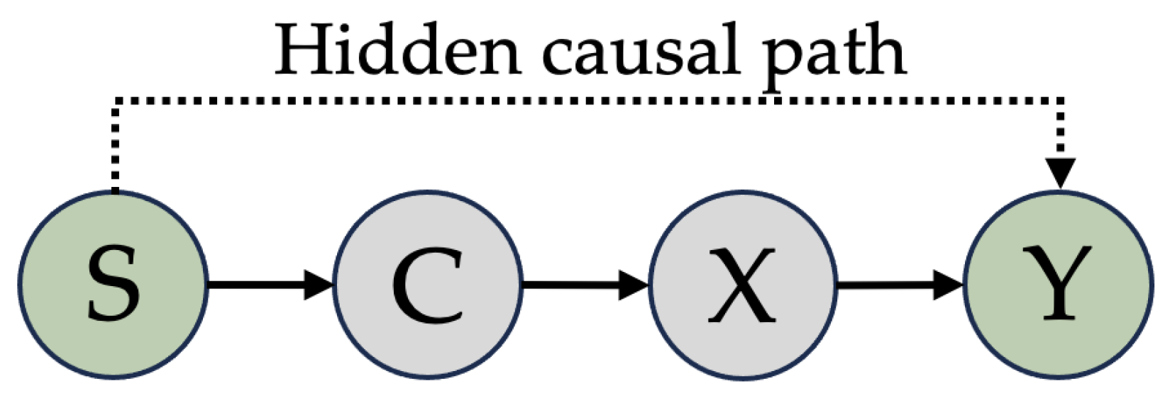
As shown in Figure 1, we construct a prediction model based on structural causality, which has four causal variables: sensitive attribute S, nonsensitive attribute C, true label Y, and node feature X, and gives the causal relationship between them. Variable C is an extrinsic variable that is not related to the sensitive attribute, which captures the data features other than the sensitive attribute. It determines the true prediction label Y through these data that are not related to the sensitive attribute. For example, when computer marking is conducted, all candidates’ sensitive information (name, student number, school, etc.) will be blocked for fair scoring. The sensitive attribute S and the nonsensitive attribute C affect the composition of node feature X together (including node information, edge connection relationship, etc.).
The prediction model constructed by integrating the causal structure enables a meticulous dissection of the underlying causes of bias within the model. This not only offers a critical theoretical framework but also facilitates a comprehensive understanding of how sensitive attributes impact the prediction results.

3.2.1. Sources of Bias

Although there is no direct causal relationship between the sensitive attribute S and the prediction label Y, there is an indirect causal path between them: S C X Y . As can be seen in Figure 2, sensitive attributes S can directly affect the composition of node features X, which in turn determine the results of prediction labels. Furthermore, the sensitive attribute S indirectly affects the prediction result Y:
P ( Y | S ) = P ( Y | X ) P ( Y | S )
Overall, bias predominantly originates from the non-causal relationship between the sensitive attribute S and the predictive label Y. Due to the inclusion of sensitive attribute S within the node feature X of the graph structure, bias inevitably emerges in the training outcomes in the prediction model. In fair GNNs, nodes update their features through neighborhood aggregation. This mechanism leads to the progressive amplification of the sensitive attribute S during the layer by layer neural network training process, ultimately undermining the fairness of the final results.
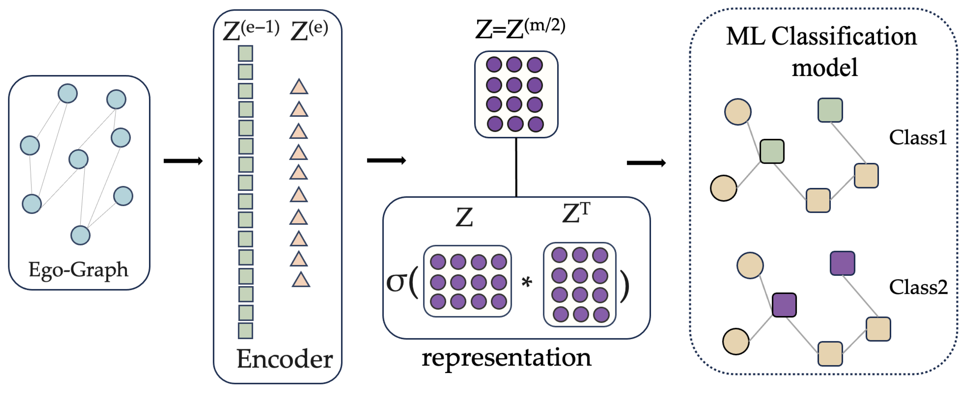
We can think about the problem from another angle. In the training process of GNNs, the encoder g(∗) aggregates information of neighbor nodes centered on nodes v i in the graph to learn the feature representation z = g(∗). The node representation z is learned in the ego-graph, that is, the balanced graph generated after the counterfactual node mixing process. The ego-graph contains graph structure information, sensitive attribute information, and other features. So, the node representation z contains the sensitive attribute features of the node v i and other nonsensitive features. After learning the node feature representation z, we classify the nodes through the classifier c(∗). After this series of operations, we can notice that the prediction label y = c(z) is made according to the ego-graph, which contains the results of the combined action of sensitive attribute S and node feature X. That is to say, although there is no direct connection between the predicted label y and the sensitive attribute S that can be seen on the causal relationship graph, there still exists a hidden relationship between them.

3.2.2. Fair Representation Learning of Debiasing

We have analyzed how sensitive attribute S is to label Y. To mitigate this bias and learn fair node representation, we propose an intervention-based counterfactual node generation method. Specifically, we intervene in the causal pathway from sensitive attribute S to prediction label Y by generating counterfactual nodes, as shown in Figure 3. For a given label Y = y, each counterfactual node enforces the sensitive attribute to take a value S S , thereby producing a diverse set of counterfactual nodes with a sensitive attribute distinct from the original node. This approach ensures the model avoids reliance on any single sensitive attribute during the prediction process.
Counterfactual nodes satisfy:
P ( Y | X ) = P ( Y | X )
In counterfactual generation, we guarantee to flip the sensitive attribute while keeping the prediction label unchanged:
P ( Y | S , X ) = P ( Y | S , X )
Therefore, after a large number of counterfactual nodes are generated, the prediction label Y will not rely too much on the sensitive attribute S:
P ( Y | S , X ) = P ( Y | X )
Thus, the causal path from S to Y is severed. Through counterfactual node generation, we mitigate bias arising from sensitive attributes while preserving the utility of the model. This approach not only generates a diverse array of counterfactual nodes but also fundamentally disrupts spurious correlations between sensitive attributes and the label, enabling the model to learn fair and interpretable node representations.

4. Methodology

In this section, we will introduce the FairCNCB model in detail, and the model architecture diagram is shown in Figure 4. Building upon causal learning theory, our model employs adversarial training to generate counterfactual nodes that are highly similar to real samples. During the node feature representation learning process, we introduce a graph representation constraint mechanism to supervise the generation of node embeddings. Finally, we reconstruct the loss function to balance the class distribution of minority sensitive attribute groups.

4.1. Counterfactual Node Generation Based on Adversarial Networks

In large-scale graph data structures, sensitive attributes have been shown to induce model unfairness. This issue is particularly pronounced in high-stakes decision-making contexts, where individuals may withhold sensitive attribute information. Consequently, minority sensitive attribute groups are disadvantaged during model training due to insufficient representation.
In fair GNNs, we can use adversarial networks to generate counterfactual nodes. The new graph network generated by combining these counterfactual nodes with real samples can reduce the dependence of target labels on sensitive attributes, thus enabling fairer decision-making. In fair graph learning, the core goal of counterfactual node generation is to generate nodes with the same target label y i , but different sensitive attributes s i for the original node v i . It can cut off the false causal path from the sensitive attribute S to the predicted result Y. Compared with direct training of the original data, counterfactual nodes generated based on the adversarial network can ensure the rationality and authenticity of the nodes. It can provide high-quality data samples for the subsequent training of fair graph neural networks.

4.1.1. Counterfactual Node Generator and Discriminator

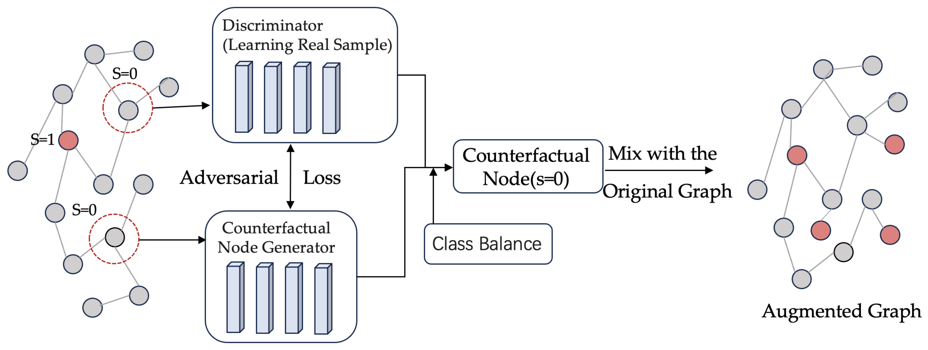
As shown in Figure 5, the adversarial network comprises two core components: a counterfactual node generator and a discriminator, which operate under mutual constraint during the training process. The generator is tasked with producing semantically plausible counterfactual nodes, while the discriminator aims to distinguish between features from the generator and real samples. This forms a dual-network architecture in which the two components engage in adversarial training. This formal adversarial network structure makes the counterfactual nodes more realistic and provides sufficient and reasonable samples in the GNN training process.
In fair graph neural networks, the counterfactual node generator ingests inputs including sensitive attributes and sample features. Through a multilayer neural architecture, it learns input node representation to generate counterfactual nodes (node features with altered sensitive attribute but identical target label) that are indistinguishable from real samples. Initially, generated counterfactual nodes may deviate significantly from real-world distributions. However, through continuous learning and updating of the neural network, the generator progressively refines its outputs to fool the discriminator. The mapping function for generating counterfactual node X′ is:
X = G ( z , x , s ) = σ L ( W L × σ L 1 ( ) + b L )
where G is the counterfactual node generator and s is the sensitive attribute. σ L denotes the activation function of layer L. W L and b L are the weight matrix and bias vectors of layer L. Random noise z usually obeys a simple distribution. In counterfactual node generation, random noise z can enable the model to generate a variety of different features of the graph structure. We also use the original feature X as part of the input of the counterfactual node generator, which guarantees the quality of the counterfactual node feature.
The discriminator takes as input two types of feature sets: real sample features X and counterfactual node features X′ generated by the counterfactual node generator. Its principal role is to discriminate between the generator features and those of the real nodes. Through iterative training, the discriminator refines its discriminative criteria by minimizing loss functions, enabling it to learn the real sample distribution. When discriminating counterfactual nodes, the discriminator optimizes the counterfactual samples through backpropagation based on the features learned from the real samples. The discriminator’s operational mechanism is defined as:
D ( x ) = σ ( V L × φ L 1 ( ) + d L )
where σ is the Sigmoid activation function and φ L 1 is the non-linear transformation of the L layer. V L and d L are the weight matrix and bias vector of layer L. When counterfactual node features are fed into the discriminator from the counterfactual node generator, the discriminator performs feature discrimination on the samples. Subsequently, it outputs a probability value ( D ( X ) [ 0 , 1 ] ) , which denotes the likelihood that the sample belongs to the real sample distribution.
m a x D D ( x )
m i n D D ( G ( z , x , s ) ) = m a x D D [ 1 D ( G ( z , x , s ) ) ]
Equations (7) and (8) indicate that when input nodes are from the real dataset, the discriminator’s optimization objective is to maximize the corresponding probability value. For counterfactual nodes generated by the counterfactual node generator, the discriminator aims to minimize this probability value. That is, a probability closer to 1 means that the discriminator classifies the sample node as real, while a value approaching 0 indicates that the node is identified as generated by the counterfactual node generator.
The max-min game between the counterfactual node generator and the discriminator drives the gradual alignment of the generated sample features with their real-world counterparts, furnishing the model with an ample supply of counterfactual samples for a subsequent classification task.

4.1.2. Adversarial Training of Counterfactual Node Generator and Discriminator

The counterfactual node generator aims to iteratively adjust its parameters, optimizing network weight and bias to minimize the distinguishability between generated counterfactual node features and real sample features. Concurrently, the discriminator must also continuously refine its parameters during training to enhance its capability of distinguishing features produced by the counterfactual node generator. In the training of fair graph neural networks, the adversarial loss function between the counterfactual node generator and discriminator effectively suppresses sensitive attribute bias, whose mathematical expression is given by:
L C F G = E x P d a t a log D ( x ) + E s s ; z P z log ( 1 D ( G ( z , x , s ) ) )
where P d a t a denotes the real sample distribution, P z denotes the random noise distribution, D is the discriminator, and G is the counterfactual node generator. When D(x) approaches 1, it indicates that the discriminator accurately identifies counterfactual node features generated by the counterfactual node generator. Conversely, when D(G(z,x,s)) approaches 1, it signifies that counterfactual samples produced by the counterfactual node generator exhibit a high degree of similarity to real samples, demonstrating significant improvement in the performance of the counterfactual node generator.

4.2. Class Balancing Mechanic

This counterfactual node generation framework based on adversarial networks effectively mitigates bias associated with sensitive attributes. Notably, this approach overlooks class imbalance among sensitive attribute groups. In fair GNN, the sample size dominance of majority groups inclines the model to prioritize learning their features during the training process. This neglect of minority sensitive attribute groups compromises the fairness of prediction outcomes. In adversarial network-based counterfactual node generation, the scarcity of minority sensitive attribute groups hinders the counterfactual node generator from learning these nodes’ features rationally.
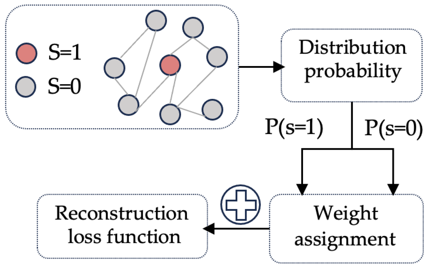
To alleviate the class imbalance problem among sensitive attribute groups and ensure that the counterfactual node generator can fairly and effectively generate high-quality representations, we introduced a class balance mechanism based on the principle of Demographic Parity. This strategy directly stems from the goal of minimizing the difference in discriminative ability between groups, and ultimately serves the principle of statistical equality and fairness. The class balancing process is visualized in Figure 6.
Within the loss function framework of adversarial training for counterfactual node generator and discriminator, we compute the weight w s for each sensitive attribute group. Given the established adversarial training loss function, we derive the inter-group weights for the sensitive attribute class as follows:
w s = l o g m a x s p ( s ) p ( s )
where p(s) is the distribution probability of the sensitive attribute s, and p(s′) is the distribution probability of the sensitive attribute s′. Then, the weights are injected into the loss function of the adversarial training:
L C B = E x P d a t a log D ( x ) + E s s ; z P z w s log ( 1 D ( G ( z , x ) ) )
In Equation (11), we integrate the weight into the adversarial training loss function to derive a novel class balancing loss function. This weight strategy directly stems from the fair goal of balancing the discriminator’s capabilities. By optimizing L C B through backpropagation, the discriminator D is forced to enhance its ability to distinguish generated samples from minority groups. Correspondingly, in order to successfully “fool” this discriminator D that is more stringent across all groups, the generator G must generate counterfactual node features of higher quality and greater difficulty in distinguishing authenticity for minority sensitive attribute groups. These improved counterfactual node features will be used more effectively in the subsequent constraints of the GNNs model, significantly reducing the dependence of its prediction results y ^ on the sensitive attribute s, thus growing closer to the statistical parity goal of P ( y ^ = 1 | s ) P ( y ^ = 1 ) .

4.3. The Fair Representation Learning

During the training of adversarial networks, it is essential to ensure that counterfactual nodes generated by the counterfactual node generator closely resemble the original sample nodes. However, such highly congruent node features may still exhibit certain bias [46]. This requires imposing constraints on the downstream classification task model to ensure the generation of fair and reliable predicted labels y ^ i .
We combine node classification tasks to judge the utility and fairness of GNNs in the training process. The target label Y is obtained by learning the node representation and adjacency matrices from the classifier f, and is expressed as:
y ^ i = f θ ( A , X )
Training the loss function of the classifier:
L pred = 1 V L v i V L y i log y ^ i + ( 1 y i ) log ( 1 y ^ i )
where | V L | denotes the number of samples in the set V L (the set of node v i ), y ^ i is the prediction label, and y i is the true label.
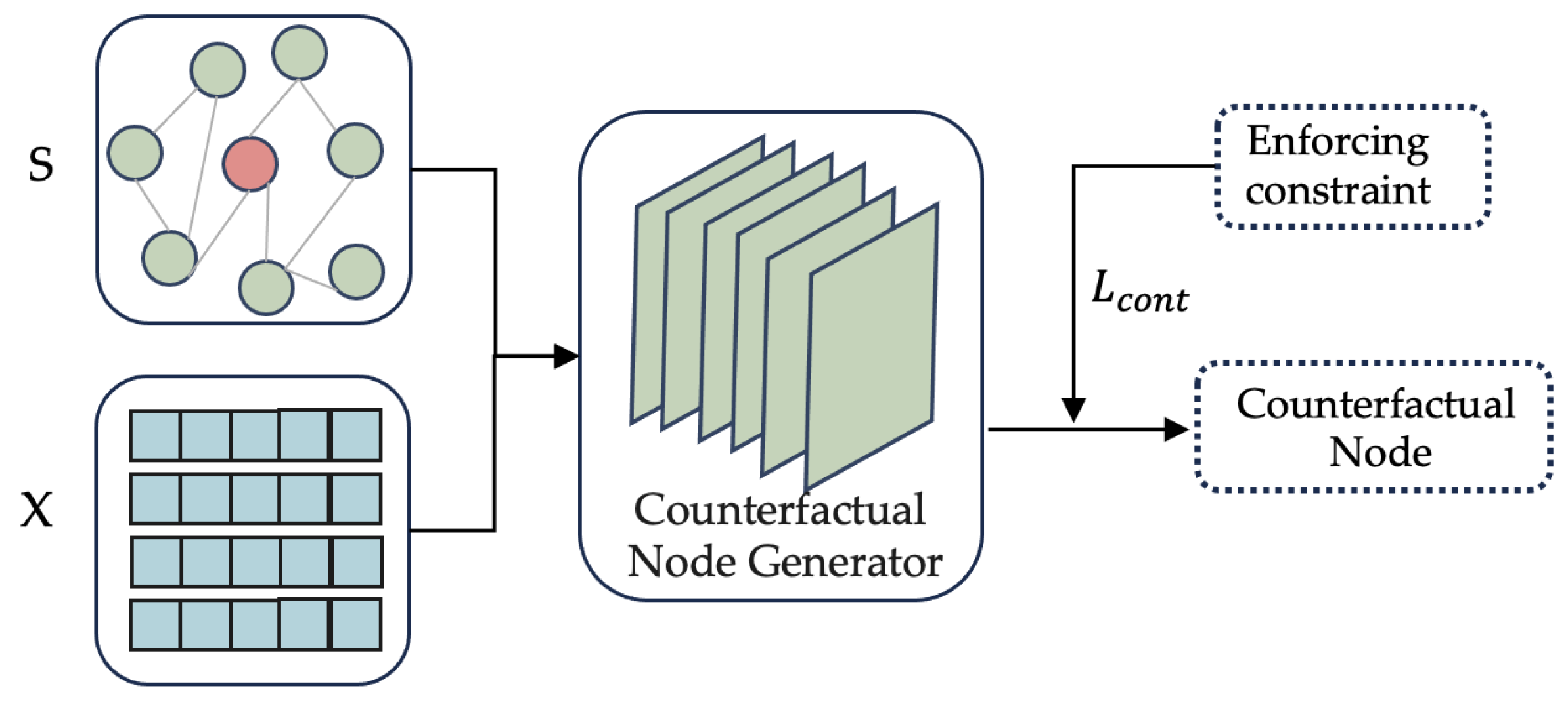
During the generation of counterfactual nodes by the counterfactual node generator, discrepancies may arise between the features of counterfactual nodes and real samples. Consequently, classifiers may exhibit predictive disparities when distinguishing between generation and real labels for these counterfactual nodes. Therefore, we need to set up a nodal constraint mechanism, as shown in Figure 7. When the sensitive attribute of the node changes, the node constraint mechanism ensures that the generated counterfactual nodes have the same prediction label as the real nodes. This approach improves fairness while preserving the utility of classification. The mathematical formulation of the constraint mechanism is:
L c o n t = E s s ; x G ( z , s ) [ ( f ( x ) , y ) ]
where ( f ( x ) , y ) is the cross-entropy of f ( x ) and y, x′ is a counterfactual node feature generated by the counterfactual node generator G.
Through backpropagation of the cross-entropy loss function, we enforce the counterfactual nodes generated by the counterfactual node generator G to align with the label y during classification tasks. If the prediction result of classifier f for counterfactual nodes disagrees with the true target label, the loss function triggers re-backpropagation, compelling generator G to strip the association between sensitive attribute s and feature x, retaining only information relevant to label y. This process imposes constraints on prediction labels, ensuring that counterfactual nodes generated by the adversarial network exhibit fairer representation. L CFG focuses on the discriminator’s ability to distinguish between real and counterfactual samples, while L cont emphasizes the label-preserving capability of counterfactual samples. These two losses jointly constrain the counterfactual node generator to produce samples that are both indistinguishable from real data and maintain label consistency, forming a complete adversarial learning framework.
When generating counterfactual nodes, an excessive number of such nodes produced by the counterfactual node generator may disrupt balance, leading to an over-weighting of minority sensitive attribute groups. After generating counterfactual nodes, we need to mix these nodes with original nodes to achieve distributional balance. Therefore, we need to control the proportion of counterfactual nodes to form a balanced graph G :
X m i n = X + η X
N ( v i ) = N ( v i )
where η [ 0 , 1 ] controls the proportion of counterfactual nodes. After constructing the new balanced graph, the connectivity between nodes changes. In Equation (16), we exclusively connect counterfactual nodes v i to their corresponding original nodes v i to avoid introducing new edges. This approach is well-suited for the simple homogeneous graph structures studied in this paper. The resulting graph preserves the original graph topology while mitigating fairness issues arising from newly generated edges.

4.4. Final Objective Function of FairCNCB

The counterfactual node generation enables the statistical mitigation of bias associated with sensitive attributes. By imposing graph information constraints on these nodes and implementing class balancing across sensitive attribute groups, we facilitate the realization of fair GNN. Algorithm 1 gives the entire training process of FairCNCB. These model approaches have their own roles and are mutually reinforcing. Therefore, putting these modules together gives us the final objective function of FairCNCB:
L C N C B = L p r e d + L c o n t + L C B
Algorithm 1: The training process of FairCNCB
Input: G = (V, A, X, S), η, Counterfactual Node Generator, Discriminator, Φ , T.
Output: prediction label y i .
     Pre-train Φ based on L p r e d
     for T do:
          Generate counterfactual nodes by Counterfactual Node Generator(Z, X );
          Determine the rationality of counterfactual nodes by Discriminator(X);
          Hybrid nodes G
          prediction label y i = Φ ( G )
           L C N C B ← Recontribution Alignment Loss;
Back-propagation;
end

5. Experiments

In this section, we performed numerous experiments on real-world datasets to assess the effectiveness of our model. Specifically, our objective is to answer the following questions:
(RQ1)
In these five evaluation indicators can FairCNCB show better performance compared to the GNN model and the fairness model?
(RQ2)
How does each module affect the working performance of the model?
(RQ3)
What are the effects of different GNN encoders in classification tasks?
(RQ4)
How do hyperparameters in the model affect FairCNCB?

5.1. Experimental Settings

5.1.1. Real-World Datasets

We conducted experiments on three widely used real-world datasets, namely German Credit, Bail, and Credit Defaulter. The statistics of the datasets can be found in Table 1. The details of the datasets are as follows:
  • German Credit [49]: The node information in the graph structure datasets is the clients. If the credit accounts of the two nodes are highly similar, they are connected. The task at hand is to classify the credit risk level as either high or low, taking into account the sensitive attribute of “gender”.
  • Bail [50]: The node information in the graph structure datasets is that of the defendant on bail. The edges between the two nodes are connected based on past criminal records and demographic similarities. The task is to classify whether a defendant is released on bail with the sensitive attribute “race”.
  • Credit Defaulter [51]: The node information in the graph structure datasets is the credit card users. The edges connected by the nodes represent the payment information if the user’s payment information is similar to each other. The task is to classify the default payment method using the sensitive attribute “age”.

5.1.2. Baselines

We compared the model with the 8 most practical and impactful methods available to verify the effectiveness of FairCNCB. We’ve divided these methods to compare into two categories: (1) classic GNNs models: GCN, GraphSAGE (SAGE for short), GAT, GIN; (2) Fair GNNs models: FairGNN, EDITS, GEAR, NIFTY, CAF. The details of each model are as follows:
  • GCN [33] proposes a very popular first-order approximate semi-supervised classification method based on spectral convolution on graphs, which can effectively encode graph network nodes.
  • GraphSAGE [34] solves the problem of unsupervised node embedding in large graphs using a function to sample and aggregate the node representations from neighbor nodes to generate an embedding.
  • GAT [52] used an attention mechanism to calculate the importance weights of neighboring nodes, capturing different types of neighbor relationships.
  • GIN [35] designed a single-shot aggregate function to learn the node representations, which can capture different graph structure data for application in graph classification tasks.
  • FairGNN [15] is grounded in adversarial learning. This approach serves to mitigate bias when dealing with limited sensitive attribute information.
  • EDITS [19] proposes a new metric to reduce bias by directly removing sensitive information.
  • GEAR [53] is an interpretable graph representation learning model based on a dual-channel graph attention mechanism, which realizes graph data generation and prediction.
  • NIFTY [17] introduces a new objective function to flip the counterfactual nodes to address the stability and fairness of GNNs.
  • CAF [25] can directly select the fair nodes to learn the real counterfactual pairs from the training samples, and can learn the fair node representation.

5.1.3. Evaluation Metrics

We regard AUC, F1 score, and accuracy as utility metrics. Statistical parity (SP) △sp and equal opportunity (EO)△eo were used to evaluate the fairness of the model.

5.1.4. Implementation Details

For the three datasets of German Credit, Credit Defaulter, and Bail, we split the datasets into train/valid/ test. For these datasets, we split the train/valid/test data using 50/25/25. We randomly initialize the hyperparameters in the experiment and search for the best hyperparameter values through the grid search method. We used the Adam optimizer [54] to train the model. Our code is available at https://github.com/yangfanzh/FairCNCB (accessed on 10 August 2025).

5.2. Performance Comparison

We integrated the node classification task across three real-world datasets to comprehensively assess the utility and fairness of FairCNCB.
Table 2 and Table 3 present the utility and fairness outcomes of each model on these datasets. The following observations can be made: (1) In comparison to other models, our FairCNCB model demonstrates outstanding utility and fairness across the three datasets, exhibiting more robust performance and competitiveness. (2) In terms of node classification utility metrics, the model outperforms the baseline model in most of the evaluation metrics across all three datasets. This performance advantage is attributable to the node representation constraints, which enforce generated counterfactual node features to closely resemble real sample features, thereby enhancing classification accuracy. (3) For the two fairness metrics, the model demonstrates substantial performance gaps with the second-best models on the German Credit and Credit Defaulter datasets, showcasing marked fairness improvements. Although both the GEAR and CAF leverage counterfactual theory for sample generation, their fairness performance lags behind our approach. This discrepancy can be attributed to our model’s explicit consideration of minority sensitive attribute group imbalance, where adaptive weighting prioritizes underrepresented groups. This mechanism directs the model’s focus toward minority groups, substantially elevating fairness outcomes.

5.3. Ablation Study

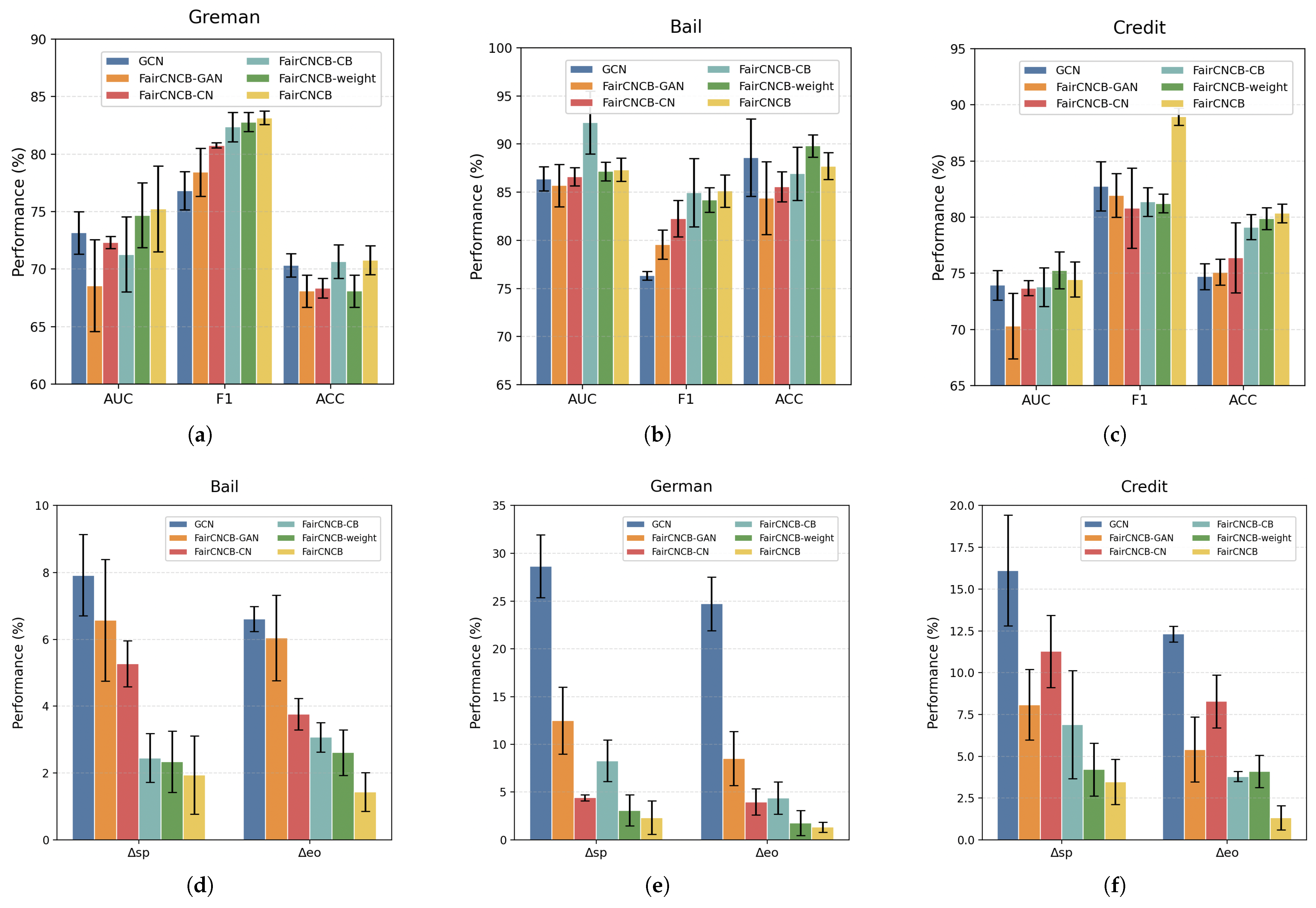
To validate the efficacy of each module within the FairCNCB framework, we developed four ablated variants: (1) FairCNCB-CN, featuring only the fairness constraint mechanism without the class balancing mechanism; (2) FairCNCB-CB, incorporating only the class balancing mechanism without the node representation constraint mechanism. (3) Removing the adversarial training mechanism, with counterfactual nodes generated by simple feature perturbations (referred to as FairCNCB-GAN). (4) Using fixed weights instead of the dynamically calculated class balance mechanism (referred to as FairCNCB-weight).
As depicted in Table 4 and Figure 8, which compares the GCN, the four ablated models, and the full FairCNCB model across three datasets. (1) The four ablated variants outperform the GCN baseline in both classification utility and fairness metrics. However, the four variants are worse than the model on the fairness metrics of the three datasets, confirming the synergistic effectiveness of the integration of the two modules. (2) FairCNCB-CN demonstrates superior fairness performance compared to FairCNCB-CB across all datasets. This is attributable to the class balancing mechanism, which assigns higher weights to minority sensitive attribute groups, thereby enhancing equity. The modules exhibit different roles in the balance of utility and fairness. FairCNCB-CB outperforms FairCNCB-CN in classification utility, primarily because: First, the node representation constraint mechanism enforces counterfactual nodes generated by the model to maintain the same labels as real samples, improving the fidelity of counterfactual node features. Second, this constraint ensures that FairCNCB-CB retains robust predictive utility while implementing fairness interventions. (3) Finally, among the two variants within the module, the model performance significantly lagged when the adversarial training mechanism was removed. This indicates that the high-quality counterfactual nodes generated by the counterfactual generator have greatly improved the classification task. When ordinary fixed weights are used in the category balance mechanism, the performance difference in utility is not significant, but fairness is somewhat reduced. Our category balance mechanism takes into account the distribution probability of sensitive attributes and uses dynamic weights to control the counterfactual node generator to focus more on generating features for minority sensitive attribute groups.

5.4. Deploying on Different Encoders

In the node classification task, we implement four state-of-the-art graph neural network (GNN) encoders (FairCNCB + GCN, FairCNCB + GraphSAGE, FairCNCB + GAT, and FairCNCB + GIN) and adopt the same utility and fairness metrics as previously defined.
Analysis of Table 5 reveals the following comparative insights: (1) GraphSAGE Encoder: Models leveraging GraphSAGE demonstrate statistically significant improvements across three utility metrics. Concurrently, they exhibit substantial enhancements in fairness indices, outperforming the baseline encoder with a notable margin. (2) GCN Encoder: The GCN-based model maintains parity with the baseline across utility metrics while achieving marked superiority in fairness metrics, indicating effective bias mitigation without compromising predictive performance. (3) GAT Encoder: A decline is observed in the F1 score for the German dataset and the ACC metric for the Bail dataset. However, this trade-off corresponds to pronounced improvements in fairness metrics, suggesting a recalibration toward equitable predictions. (4) GIN Encoder: While marginally underperforming in F1 scores, the GIN-based model demonstrates robust performance in fairness metrics, underscoring its efficacy in balancing predictive accuracy and equity. These results collectively indicate that the proposed framework yields modest yet consistent improvements in classification utility while achieving statistically significant advancements in fairness metrics. This dual efficacy is primarily attributable to the model’s counterfactual node generation mechanism and adaptive class balancing strategy, which synergistically mitigate bias propagation.

5.5. Parametric Analysis

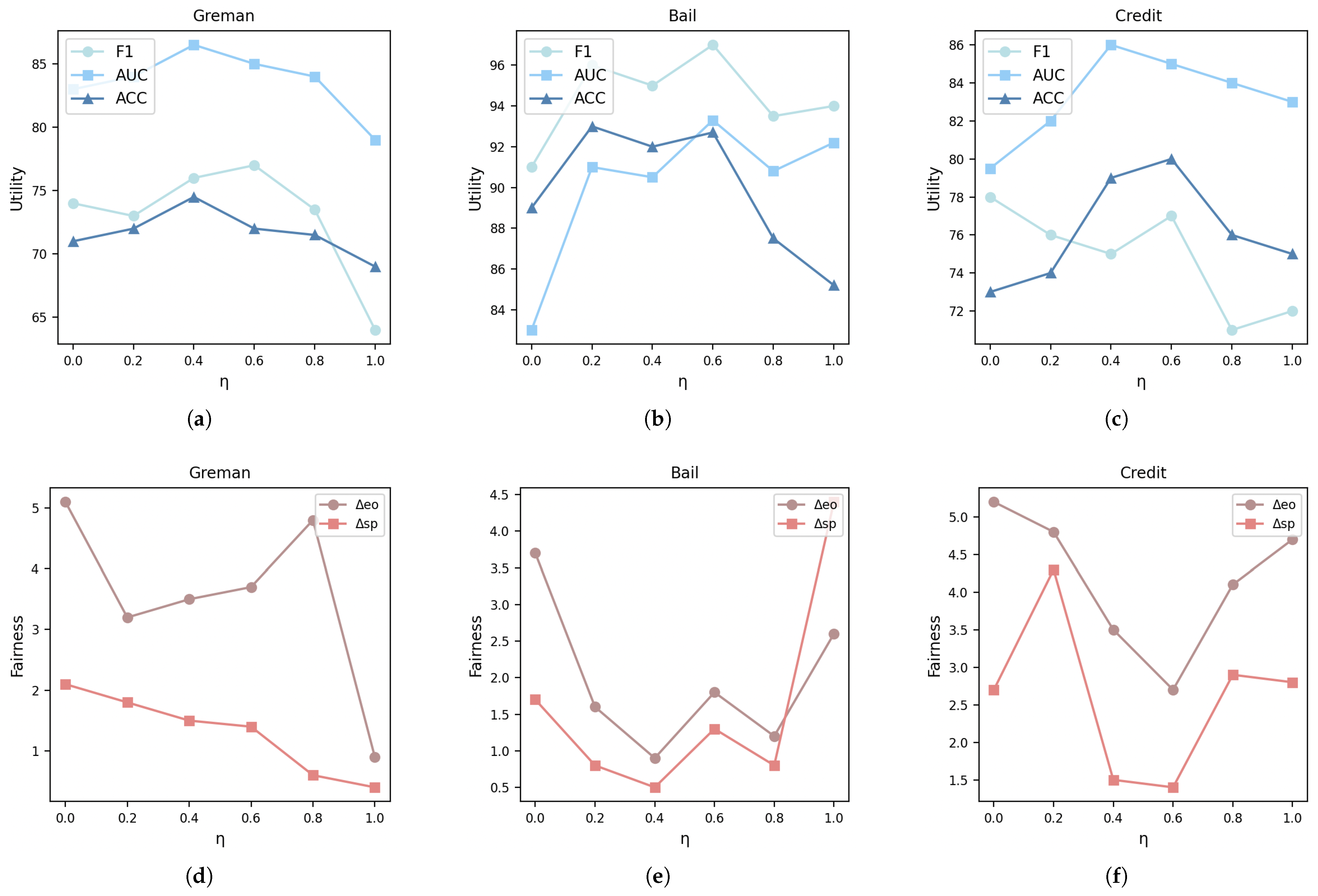
In the process of generating counterfactual nodes via adversarial networks, we introduce a hyperparameter η to control the mixing ratio of counterfactual nodes. To address RQ4, we vary η from 0 to 1. As shown in Figure 9, when η exceeds 0.8, the fairness indices of the three datasets significantly improve, but the node classification utility indices remain low. Conversely, when η is below 0.2, both the utility and fairness indices across all datasets are suboptimal. Notably, within the η range of 0.4–0.6, although some performance metrics exhibit periodic fluctuations, the comprehensive balance between node classification utility and fairness tends to stabilize. Specifically, when η is set to 0.5, the model not only achieves the desired target for both utility and fairness indices but also optimizes the overall performance of the FairCNCB model, demonstrating an ideal trade-off.

6. Conclusions

In this study, we propose a novel method to address fairness issues in graph neural networks (GNNs) by leveraging counterfactual-node-generation via adversarial networks and a balancing strategy for minority sensitive attribute groups. It is found that there is a class imbalance among the minority sensitive attribute groups, which leads to the unfairness of GNN prediction results. In view of this, the FairCNCB model we propose has shown excellent performance in dealing with the fairness problem of GNNs. Informed by causal theory, we effectively mitigate bias stemming from sensitive attributes through counterfactual-node generation via adversarial networks. To further enhance fairness, we reconstruct the loss function to enforce class balance for minority sensitive attribute groups. The two modules are organically and flexibly combined to achieve a fair GNN architecture. The experimental results fully show that the FairCNCB model has reached the current state-of-the-art level in terms of classification utility and fairness on three datasets. Looking ahead, there are still many aspects to explore. This study focuses on Homogeneous Graphs, but Heterogeneous Graphs are widely used as more complex structures in many real-world applications. Therefore, it is important to expand the existing model to diverse types of graph structure domains. The sensitive attributes examined in this article are all binary, which is impractical in many high-stakes decision-making systems. Going forward, this framework could be extended to accommodate multi-dimensional sensitive attributes.

Author Contributions

Conceptualization, Z.X. and Y.Z.; writing-review and editing, Z.X. and Y.Z.; visualization, Z.X. and Y.Z.; formal analysis, K.W. and D.L. All authors have read and agreed to the published version of the manuscript.

Funding

This research was supported by the Basic Construction Funds within the Budget of Jilin Province in 2024 (No. 2024C008-7).

Institutional Review Board Statement

Not applicable.

Informed Consent Statement

Not applicable.

Data Availability Statement

All the datasets in the paper can be downloaded from References [49,50,51].

Acknowledgments

We would like to thank Changchun University, College of Computer Science and Technology for Non-Point Source Pollution Control in Agriculture for providing the research environment and computing resources.

Conflicts of Interest

The authors state that there are no conflicts of interest.

References

  1. Zhang, S.; Ni, W.W.; Fu, N. Community-Preserving Social Graph Release with Node Differential Privacy. J. Comput. Sci. Technol. 2023, 38, 1369–1386. [Google Scholar] [CrossRef]
  2. Berk, R. Accuracy and fairness for juvenile justice risk assessments. J. Empir. Leg. Stud. 2019, 16, 175–194. [Google Scholar] [CrossRef]
  3. Liu, Y.C.; Tian, J.; Glaser, N.; Kira, Z. When2com: Multi-agent perception via communication graph grouping. In Proceedings of the IEEE/CVF Conference on Computer Vision and Pattern Recognition, Seattle, WA, USA, 13–19 June 2020; pp. 4106–4115. [Google Scholar]
  4. Martinez-Riano, A.; Wang, S.; Boeing, S.; Minoughan, S.; Casal, A.; Spillane, K.M.; Ludewig, B.; Tolar, P. Long-term retention of antigens in germinal centers is controlled by the spatial organization of the follicular dendritic cell network. Nat. Immunol. 2023, 24, 1281–1294. [Google Scholar] [CrossRef]
  5. Fofanah, A.J.; Leigh, A.O. EATSA-GNN: Edge-Aware and Two-Stage attention for enhancing graph neural networks based on teacher–student mechanisms for graph node classification. Neurocomputing 2025, 612, 128686. [Google Scholar] [CrossRef]
  6. Ma, T.; Wang, H.; Zhang, L.; Tian, Y.; Al-Nabhan, N. Graph classification based on structural features of significant nodes and spatial convolutional neural networks. Neurocomputing 2021, 423, 639–650. [Google Scholar] [CrossRef]
  7. Pang, J.; Gu, Y.; Xu, J.; Yu, G. Semi-supervised multi-graph classification using optimal feature selection and extreme learning machine. Neurocomputing 2018, 277, 89–100. [Google Scholar] [CrossRef]
  8. Said, A.; Janjua, M.U.; Hassan, S.U.; Muzammal, Z.; Saleem, T.; Thaipisutikul, T.; Tuarob, S.; Nawaz, R. Detailed analysis of Ethereum network on transaction behavior, community structure and link prediction. PeerJ Comput. Sci. 2021, 7, e815. [Google Scholar] [CrossRef]
  9. Li, X.; Shang, Y.; Cao, Y.; Li, Y.; Tan, J.; Liu, Y. Type-aware anchor link prediction across heterogeneous networks based on graph attention network. In Proceedings of the AAAI Conference on Artificial Intelligence, New York, NY, USA, 7–12 February 2020; Volume 34, pp. 147–155. [Google Scholar]
  10. Dai, E.; Cui, L.; Wang, Z.; Tang, X.; Wang, Y.; Cheng, M.; Yin, B.; Wang, S. A unified framework of graph information bottleneck for robustness and membership privacy. In Proceedings of the 29th ACM SIGKDD Conference on Knowledge Discovery and Data Mining, Long Beach, CA, USA, 6–10 August 2023; pp. 368–379. [Google Scholar]
  11. Köse, Ö.D.; Shen, Y. Fairness-aware node representation learning. arXiv 2021, arXiv:2106.05391. [Google Scholar]
  12. Ma, J.; Deng, J.; Mei, Q. Subgroup generalization and fairness of graph neural networks. Adv. Neural Inf. Process. Syst. 2021, 34, 1048–1061. [Google Scholar]
  13. Beutel, A.; Chen, J.; Zhao, Z.; Chi, E.H. Data decisions and theoretical implications when adversarially learning fair representations. arXiv 2017, arXiv:1707.00075. [Google Scholar]
  14. Mehrabi, N.; Morstatter, F.; Saxena, N.; Lerman, K.; Galstyan, A. A survey on bias and fairness in machine learning. ACM Comput. Surv. (CSUR) 2021, 54, 1–35. [Google Scholar] [CrossRef]
  15. Dai, E.; Wang, S. Say no to the discrimination: Learning fair graph neural networks with limited sensitive attribute information. In Proceedings of the 14th ACM International Conference on Web Search and Data Mining, Virtual Event, 8–12 March 2021; pp. 680–688. [Google Scholar]
  16. Bao, H.; Dong, L.; Wang, W.; Yang, N.; Piao, S.; Wei, F. Fine-tuning pretrained transformer encoders for sequence-to-sequence learning. Int. J. Mach. Learn. Cybern. 2024, 15, 1711–1728. [Google Scholar] [CrossRef]
  17. Agarwal, C.; Lakkaraju, H.; Zitnik, M. Towards a unified framework for fair and stable graph representation learning. In Proceedings of the Uncertainty in Artificial Intelligence, PMLR, Online, 27–30 July 2021; pp. 2114–2124. [Google Scholar]
  18. Dong, Y.; Kang, J.; Tong, H.; Li, J. Individual fairness for graph neural networks: A ranking based approach. In Proceedings of the 27th ACM SIGKDD Conference on Knowledge Discovery & Data Mining, Singapore, 14–18 August 2021; pp. 300–310. [Google Scholar]
  19. Dong, Y.; Liu, N.; Jalaian, B.; Li, J. Edits: Modeling and mitigating data bias for graph neural networks. In Proceedings of the ACM Web Conference 2022, Lyon, France, 25–29 April 2022; pp. 1259–1269. [Google Scholar]
  20. Dong, Y.; Ma, J.; Wang, S.; Chen, C.; Li, J. Fairness in graph mining: A survey. IEEE Trans. Knowl. Data Eng. 2023, 35, 10583–10602. [Google Scholar] [CrossRef]
  21. Dong, Y.; Zhang, B.; Yuan, Y.; Zou, N.; Wang, Q.; Li, J. Reliant: Fair knowledge distillation for graph neural networks. In Proceedings of the 2023 SIAM International Conference on Data Mining (SDM), Minneapolis, MI, USA, 27–29 April 2023; SIAM: Bangkok, Thailand, 2023; pp. 154–162. [Google Scholar]
  22. Ma, J.; Guo, R.; Wan, M.; Yang, L.; Zhang, A.; Li, J. Learning fair node representations with graph counterfactual fairness. In Proceedings of the Fifteenth ACM International Conference on Web Search and Data Mining, Virtual Event, AZ, USA, 21–25 February 2022; pp. 695–703. [Google Scholar]
  23. Wang, Y.; Zhao, Y.; Dong, Y.; Chen, H.; Li, J.; Derr, T. Improving fairness in graph neural networks via mitigating sensitive attribute leakage. In Proceedings of the 28th ACM SIGKDD Conference on Knowledge Discovery and Data Mining, Washington, DC, USA, 14–18 August 2022; pp. 1938–1948. [Google Scholar]
  24. Dai, E.; Zhao, T.; Zhu, H.; Xu, J.; Guo, Z.; Liu, H.; Tang, J.; Wang, S. A comprehensive survey on trustworthy graph neural networks: Privacy, robustness, fairness, and explainability. Mach. Intell. Res. 2024, 21, 1011–1061. [Google Scholar] [CrossRef]
  25. Guo, Z.; Li, J.; Xiao, T.; Ma, Y.; Wang, S. Towards fair graph neural networks via graph counterfactual. In Proceedings of the 32nd ACM International Conference on Information and Knowledge Management, Birmingham, UK, 21–25 October 2023; pp. 669–678. [Google Scholar]
  26. Song, W.; Dong, Y.; Liu, N.; Li, J. Guide: Group equality informed individual fairness in graph neural networks. In Proceedings of the 28th ACM SIGKDD Conference on Knowledge Discovery and Data Mining, Washington, DC, USA, 14–18 August 2022; pp. 1625–1634. [Google Scholar]
  27. Rahman, T.; Surma, B.; Backes, M.; Zhang, Y. Fairwalk: Towards fair graph embedding. In Proceedings of the 28th International Joint Conference on Artificial Intelligen, Macao, China, 10–16 August 2019. [Google Scholar]
  28. Zhao, T.; Zhang, X.; Wang, S. Graphsmote: Imbalanced node classification on graphs with graph neural networks. In Proceedings of the 14th ACM International Conference on Web Search and Data Mining, Virtual Event, Israel, 8–12 March 2021; pp. 833–841. [Google Scholar]
  29. Mukherjee, D.; Yurochkin, M.; Banerjee, M.; Sun, Y. Two simple ways to learn individual fairness metrics from data. In Proceedings of the International Conference on Machine Learning, PMLR, Online, 13–18 July 2020; pp. 7097–7107. [Google Scholar]
  30. Fan, S.; Wang, X.; Mo, Y.; Shi, C.; Tang, J. Debiasing graph neural networks via learning disentangled causal substructure. Adv. Neural Inf. Process. Syst. 2022, 35, 24934–24946. [Google Scholar]
  31. Jiang, W.; Liu, H.; Xiong, H. Survey on trustworthy graph neural networks: From a causal perspective. arXiv 2023, arXiv:2312.12477. [Google Scholar]
  32. Sui, Y.; Wang, X.; Wu, J.; Lin, M.; He, X.; Chua, T.S. Causal attention for interpretable and generalizable graph classification. In Proceedings of the 28th ACM SIGKDD Conference on Knowledge Discovery and Data Mining, Washington, DC, USA, 14–18 August 2022; pp. 1696–1705. [Google Scholar]
  33. Kipf, T.N.; Welling, M. Semi-supervised classification with graph convolutional networks. arXiv 2016, arXiv:1609.02907. [Google Scholar]
  34. Hamilton, W.; Ying, Z.; Leskovec, J. Inductive representation learning on large graphs. In Proceedings of the 31st International Conference on Neural Information Processing Systems, Long Beach, CA, USA, 4–9 December 2017; Volume 30. [Google Scholar]
  35. Xu, K.; Hu, W.; Leskovec, J.; Jegelka, S. How powerful are graph neural networks? arXiv 2018, arXiv:1810.00826. [Google Scholar]
  36. Xiao, T.; Wang, D. A general offline reinforcement learning framework for interactive recommendation. In Proceedings of the AAAI Conference on Artificial Intelligence, Online, 2–9 February 2021; Volume 35, pp. 4512–4520. [Google Scholar]
  37. Jin, G.; Wang, Q.; Zhu, C.; Feng, Y.; Huang, J.; Zhou, J. Addressing crime situation forecasting task with temporal graph convolutional neural network approach. In Proceedings of the 2020 12th International Conference on Measuring Technology and Mechatronics Automation (ICMTMA), Phuket, Thailand, 28–29 February 2020; IEEE: New York, NY, USA, 2020; pp. 474–478. [Google Scholar]
  38. Diana, E.; Gill, W.; Kearns, M.; Kenthapadi, K.; Roth, A. Minimax group fairness: Algorithms and experiments. In Proceedings of the 2021 AAAI/ACM Conference on AI, Ethics, and Society, Virtual Event, USA, 19–21 May 2021; pp. 66–76. [Google Scholar]
  39. Fleisher, W. What’s fair about individual fairness? In Proceedings of the 2021 AAAI/ACM Conference on AI, Ethics, and Society, Virtual Event, USA, 19–21 May 2021; pp. 480–490. [Google Scholar]
  40. Sharifi-Malvajerdi, S.; Kearns, M.; Roth, A. Average individual fairness: Algorithms, generalization and experiments. In Proceedings of the 33rd Conference on Neural Information Processing Systems (NeurIPS 2019), Vancouver, BC, Canada, 8–14 December 2019; Volume 32. [Google Scholar]
  41. Chiappa, S. Path-specific counterfactual fairness. In Proceedings of the AAAI Conference on Artificial Intelligence, Honolulu, HI, USA, 27 January–1 February 2019; Volume 33, pp. 7801–7808. [Google Scholar]
  42. Kusner, M.J.; Loftus, J.; Russell, C.; Silva, R. Counterfactual fairness. In Proceedings of the 31st International Conference on Neural Information Processing Systems, Long Beach, CA, USA, 4–9 December 2017; Volume 30. [Google Scholar]
  43. Makhlouf, K.; Zhioua, S.; Palamidessi, C. Survey on causal-based machine learning fairness notions. arXiv 2020, arXiv:2010.09553. [Google Scholar]
  44. Zečević, M.; Dhami, D.S.; Veličković, P.; Kersting, K. Relating graph neural networks to structural causal models. arXiv 2021, arXiv:2109.04173. [Google Scholar]
  45. Lin, W.; Lan, H.; Li, B. Generative causal explanations for graph neural networks. In Proceedings of the International Conference on Machine Learning, PMLR, Virtual, 18–24 July 2021; pp. 6666–6679. [Google Scholar]
  46. Wang, X.; Wu, Y.; Zhang, A.; Feng, F.; He, X.; Chua, T.S. Reinforced causal explainer for graph neural networks. IEEE Trans. Pattern Anal. Mach. Intell. 2022, 45, 2297–2309. [Google Scholar] [CrossRef] [PubMed]
  47. Wang, L.; Adiga, A.; Chen, J.; Sadilek, A.; Venkatramanan, S.; Marathe, M. Causalgnn: Causal-based graph neural networks for spatio-temporal epidemic forecasting. In Proceedings of the AAAI Conference on Artificial Intelligence, Virtual, 22 February–1 March 2022; Volume 36, pp. 12191–12199. [Google Scholar]
  48. Pearl, J. Causality; Cambridge University Press: Cambridge, UK, 2009. [Google Scholar]
  49. Asuncion, A.; Newman, D. UCI Machine Learning Repository; University of California: Irvine, CA, USA, 2007. [Google Scholar]
  50. Jordan, K.L.; Freiburger, T.L. The effect of race/ethnicity on sentencing: Examining sentence type, jail length, and prison length. J. Ethn. Crim. Justice 2015, 13, 179–196. [Google Scholar] [CrossRef]
  51. Yeh, I.C.; Lien, C.h. The comparisons of data mining techniques for the predictive accuracy of probability of default of credit card clients. Expert Syst. Appl. 2009, 36, 2473–2480. [Google Scholar] [CrossRef]
  52. Veličković, P.; Cucurull, G.; Casanova, A.; Romero, A.; Lio, P.; Bengio, Y. Graph attention networks. arXiv 2017, arXiv:1710.10903. [Google Scholar]
  53. Wang, H.; Wang, J.; Wang, J.; Zhao, M.; Zhang, W.; Zhang, F.; Xie, X.; Guo, M. Graphgan: Graph representation learning with generative adversarial nets. In Proceedings of the AAAI Conference on Artificial Intelligence, New Orleans, LA, USA, 2–7 February 2018; Volume 32. [Google Scholar]
  54. Kingma, D.P.; Ba, J. Adam: A method for stochastic optimization. arXiv 2014, arXiv:1412.6980. [Google Scholar]
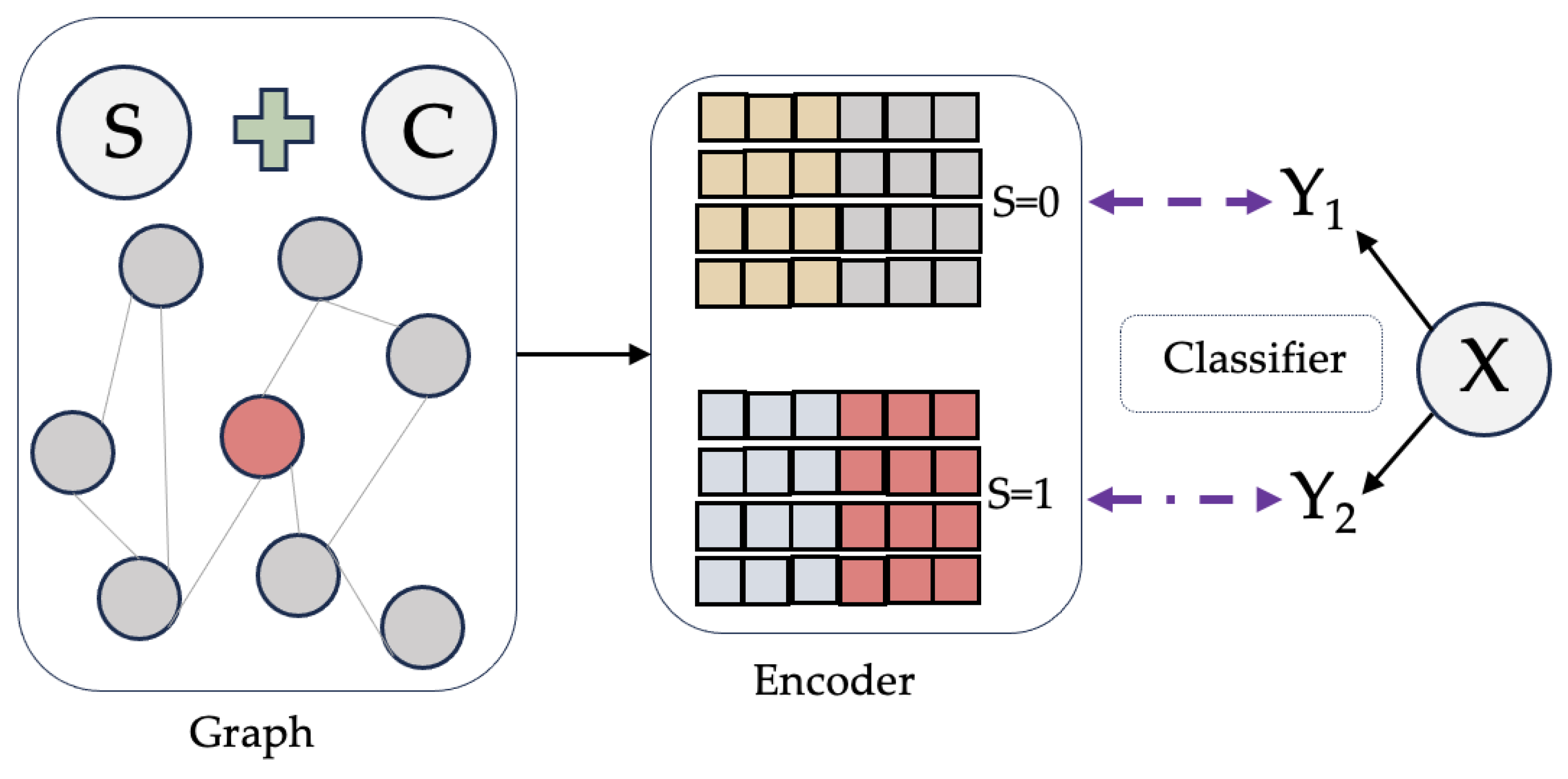
Figure 1. Combined the causal learning and classification model.
Information 16 00704 g001
Figure 2. The node classification process with causal relationships.
Information 16 00704 g002
Figure 3. The hidden causal path between the sensitive attribute and prediction label.
Information 16 00704 g003
Figure 4. The overview of proposed FairCNCB model.
Information 16 00704 g004
Figure 5. Counterfactual node Generator and Discriminator.
Information 16 00704 g005
Figure 6. The class balancing process.
Information 16 00704 g006
Figure 7. The constraint on prediction labels.
Information 16 00704 g007
Figure 8. The error bar chart of the ablation experiment results: (a) The utility results on the German dataset. (b) The utility results on the Bail dataset. (c) The utility results on the Credit dataset. (d) The fairness results on the German dataset. (e) The fairness results on the Bail dataset. (f) The fairness results on the Credit dataset.
Information 16 00704 g008
Figure 9. Experimental results of hyperparameter analysis: (a) The utility results on the German dataset. (b) The utility results on the Bail dataset (c) The utility results on the Credit dataset. (d) The fairness results on the German dataset. (e) The fairness results on the Bail dataset (f) The fairness results on the Credit dataset.
Information 16 00704 g009
Table 1. The Statistic of Datasets.
DatasetGerman CreditBailCredit Defaulter
Nodes100018,87630,000
Edges22,242321,3081,436,858
Attributes271813
Sens.GenderRaceAge
LabelCredit statusBail decisionFuture default
Table 2. The performance of FairCNCB on German, Credit, and Bail with respect to utility and fairness in the classic GNN model. ↑ represents the larger, the better, while ↓ represents the smaller, the better. Each experimental result is obtained from 10 repeated experiments.
DatasetsMetrics (%)GATGINSAGEFairCNCB
GermanAUC (↑)70.84 ± 0.7173.59 ± 1.3673.43 ± 1.8175.25 ± 3.74
F1 (↑)87.62 ± 1.5782.32 ± 1.8282.38 ± 1.1283.16 ± 0.58
ACC (↑)71.63 ± 0.8272.56 ± 0.8770.83 ± 0.5970.78 ± 1.25
△sp (↓)11.27 ± 1.9317.46 ± 6.3126.35 ± 5.172.23 ± 1.74
△eo (↓)9.03 ± 0.3110.28 ± 7.3617.39 ± 3.281.32 ± 0.53
BailAUC (↑)76.94 ± 1.1685.27 ± 0.4291.38 ± 0.4687.34 ± 1.20
F1 (↑)83.59 ± 2.0677.83 ± 0.4981.17 ± 1.3285.13 ± 1.69
ACC (↑)85.02 ± 1.3582.71 ± 0.8288.72 ± 4.2587.72 ± 1.38
△sp (↓)4.73 ± 0.598.53 ± 1.273.52 ± 2.521.94 ± 1.17
△eo (↓)7.86 ± 0.318.39 ± 0.651.92 ± 3.921.43 ± 0.58
CreditAUC (↑)70.94 ± 1.0872.53 ± 2.3771.67 ± 1.3874.45 ± 1.56
F1 (↑)85.03 ± 1.4183.15 ± 0.1483.92 ± 1.1783.35 ± 0.77
ACC (↑)79.36 ± 1.1777.96 ± 0.1875.27 ± 2.4580.35 ± 0.83
△sp (↓)7.91 ± 2.495.36 ± 1.1216.39 ± 1.983.47 ± 1.36
△eo (↓)11.58 ± 3.113.46 ± 2.7312.17 ± 4.323.31 ± 0.72
Table 3. The performance of FairCNCB on German, Credit, and Bail with respect to utility and fairness in the fair GNN model. ↑ represents the larger, the better, while ↓ represents the smaller, the better.
DatasetsMetrics (%)FairGNNEDITSGEARNIFTYCAFFairCNCB
GermanAUC (↑)69.52 ± 1.0771.01 ± 1.3070.42 ± 0.8170.32 ± 4.4271.87 ± 1.3375.25 ± 3.74
F1 (↑)80.71 ± 1.3182.43 ± 0.6980.02 ± 1.1381.98 ± 0.8282.16 ± 0.2283.16 ± 0.58
ACC (↑)68.45 ± 2.8368.73 ± 1.0468.42 ± 0.7365.53 ± 3.9468.39 ± 1.0670.78 ± 1.25
△sp (↓)11.55 ± 1.938.30 ± 3.105.48 ± 1.4915.08 ± 8.826.60 ± 1.662.23 ± 1.74
△eo (↓)6.18 ± 2.173.75 ± 3.306.81 ± 0.1612.56 ± 8.601.58 ± 1.141.32 ± 0.53
BailAUC (↑)85.69 ± 0.7785.73 ± 3.0289.60 ± 0.1688.51 ± 3.0891.39 ± 0.3487.34 ± 1.2
F1 (↑)83.47 ± 1.3279.97 ± 1.2980.00 ± 0.3179.92 ± 4.0983.09 ± 0.9885.13 ± 1.69
ACC (↑)85.81 ± 0.6483.26 ± 0.4085.20 ± 0.2684.61 ± 1.2785.91 ± 1.7887.72 ± 1.38
△sp (↓)2.09 ± 0.483.93 ± 0.595.80 ± 0.173.82 ± 1.092.29 ± 1.061.94 ± 1.17
△eo (↓)1.91 ± 0.352.30 ± 0.771.90 ± 0.235.47 ± 1.791.17 ± 0.521.43 ± 0.58
CreditAUC (↑)74.56 ± 1.3870.16 ± 0.6074.00 ± 0.0871.92 ± 0.1973.42 ± 1.8974.45 ± 1.56
F1 (↑)81.61 ± 0.8481.44 ± 0.2083.5 ± 0.0881.99 ± 0.6383.63 ± 0.8983.35 ± 0.77
ACC (↑)78.97 ± 1.3072.67 ± 0.9176.55 ± 0.1177.74 ± 3.9778.41 ± 2.9080.35 ± 0.83
△sp (↓)4.79 ± 0.599.13 ± 1.201.04 ± 0.1312.40 ± 1.628.63 ± 2.133.47 ± 1.36
△eo (↓)7.14 ± 2.867.88 ± 1.008.60 ± 0.1810.09 ± 1.556.85 ± 1.553.31 ± 0.72
Table 4. Ablation study results. ↑ represents the larger, the better, while ↓ represents the smaller, the better.
DatasetsMetrics (%)GCNFairCNCB-GANFairCNCB-CNFairCNCB-CBFairCNCB-WeightFairCNCB
GermanAUC (↑)73.16 ± 1.8668.57 ± 4.0072.32 ± 0.5471.28 ± 3.2774.69 ± 2.8175.25 ± 3.74
F1 (↑)76.84 ± 1.6578.43 ± 2.1080.76 ± 0.2282.36 ± 1.2782.79 ± 0.8383.16 ± 0.58
ACC (↑)71.76+1.0268.09 ± 1.4068.36 ± 0.8670.67 ± 1.4671.68 ± 1.3970.78 ± 1.25
△sp (↓)28.65 ± 3.2612.50 ± 3.504.41 ± 0.328.28 ± 2.173.07 ± 1.632.23 ± 1.74
△eo (↓)24.73 ± 2.828.50 ± 2.383.97 ± 1.384.38 ± 1.691.75 ± 1.321.32 ± 0.53
BailAUC (↑)86.38 ± 1.2685.71 ± 2.2086.62 ± 0.9592.26 ± 3.7387.17 ± 0.9687.34 ± 1.2
F1 (↑)76.33 ± 1.4779.55 ± 1.5182.25 ± 1.8984.96 ± 4.5384.20 ± 1.2885.13 ± 1.69
ACC (↑)88.61 ± 4.0384.39 ± 1.7785.57 ± 1.5586.93 ± 2.7689.81 ± 1.1487.72 ± 1.38
△sp (↓)7.92 ± 1.216.57 ± 1.825.27 ± 0.692.45 ± 0.732.34 ± 0.921.94 ± 1.17
△eo (↓)6.61 ± 0.376.04 ± 1.283.76 ± 0.473.07 ± 0.442.61 ± 0.781.43 ± 0.58
CreditAUC (↑)72.94 ± 1.3270.31 ± 2.9373.68 ± 0.6773.78 ± 1.7275.27 ± 1.6374.45 ± 1.56
F1 (↑)82.75 ± 2.281.95 ± 1.2380.82 ± 3.5781.36 ± 1.2881.22 ± 0.8383.35 ± 0.77
ACC (↑)75.82 ± 3.5675.11 ± 1.1576.4 ± 4.5279.12 ± 1.1279.88 ± 0.9880.35 ± 0.83
△sp (↓)16.13 ± 3.318.09 ± 2.1111.28 ± 2.166.89 ± 3.234.21 ± 1.583.47 ± 1.36
△eo (↓)12.32 ± 0.485.41 ± 1.958.29 ± 1.583.79 ± 2.314.10 ± 0.963.31 ± 0.72
Table 5. The results of different encoders in the node classification task. ↑ represents the larger, the better, while ↓ represents the smaller, the better.
DatasetsMetrics (%)GCNFairGCNSAGEFairSAGEGATFairGATGINFairGIN
GermanAUC (↑)73.16 ± 1.8675.42 ± 1.2273.43 ± 1.8174.37 ± 0.7170.84 ± 0.7172.63 ± 1.0273.59 ± 1.3676.25 ± 2.19
F1 (↑)76.84 ± 1.6583.79 ± 2.7382.38 ± 1.1284.54 ± 1.0287.62 ± 1.5785.39 ± 2.2382.32 ± 1.8280.58 ± 0.44
ACC (↑)71.76 ± 1.0277.19 ± 0.3170.83 ± 0.5980.12 ± 1.1971.63 ± 0.8276.17 ± 1.0372.56 ± 0.8774.31 ± 1.93
△sp (↓)28.65 ± 3.262.4 ± 0.7726.35 ± 5.171.91 ± 0.5911.27 ± 1.934.58 ± 1.9417.46 ± 6.312.83 ± 1.19
△eo (↓)24.73 ± 2.821.91 ± 0.2117.39 ± 3.282.77 ± 1.039.03 ± 0.315.27 ± 1.3310.28 ± 7.362.84 ± 1.92
BailAUC (↑)86.38 ± 1.2686.73 ± 1.1791.38 ± 0.4688.49 ± 3.1276.94 ± 1.1679.11 ± 0.7285.27 ± 0.4281.26 ± 0.75
F1 (↑)76.33 ± 1.4777.67 ± 1.1881.17 ± 1.3281.39 ± 0.9183.59 ± 2.0685.51 ± 1.1977.83 ± 0.4979.31 ± 2.16
ACC (↑)88.61 ± 4.0385.92 ± 2.0388.72 ± 4.2589.76 ± 1.8185.02 ± 1.3583.41 ± 1.5582.71 ± 0.8274.69 ± 0.71
△sp (↓)7.92 ± 1.215.43 ± 2.843.52 ± 2.521.89 ± 1.274.73 ± 0.594.41 ± 1.038.53 ± 1.274.31 ± 2.11
△eo (↓)6.61 ± 0.371.40 ± 1.261.92 ± 3.921.69 ± 0.737.86 ± 0.313.77 ± 2.098.39 ± 0.655.47 ± 0.93
CreditAUC (↑)72.94 ± 1.3276.59 ± 0.1871.67 ± 1.3877.42 ± 1.1270.94 ± 1.0872.37 ± 1.4872.53 ± 2.3776.82 ± 0.44
F1 (↑)82.75 ± 2.283.71 ± 1.1883.92 ± 1.1785.33 ± 2.0285.03 ± 1.4186.26 ± 0.8183.15 ± 0.1482.39 ± 0.41
ACC (↑)75.82 ± 3.5680.81 ± 0.1575.27 ± 2.4579.04 ± 2.2679.36 ± 1.1782.69 ± 1.3677.96 ± 0.1880.53 ± 1.87
△sp (↓)16.13 ± 3.313.79 ± 0.3116.39 ± 1.983.77 ± 1.037.91 ± 2.493.79 ± 1.325.36 ± 1.122.23 ± 0.33
△eo (↓)12.32 ± 0.483.49 ± 0.9412.17 ± 4.322.67 ± 0.7411.58 ± 3.113.55 ± 2.193.46 ± 2.731.83 ± 0.27
Disclaimer/Publisher’s Note: The statements, opinions and data contained in all publications are solely those of the individual author(s) and contributor(s) and not of MDPI and/or the editor(s). MDPI and/or the editor(s) disclaim responsibility for any injury to people or property resulting from any ideas, methods, instructions or products referred to in the content.