Deep Learning-Enhanced Ocean Acoustic Tomography: A Latent Feature Fusion Framework for Hydrographic Inversion with Source Characteristic Embedding

Abstract

Ocean Acoustic Tomography (OAT) is an important marine remote sensing technique used for inverting large-scale ocean environmental parameters, but traditional methods face challenges in computational complexity and environmental interference. This paper proposes a causal analysis-driven AI FOR SCIENCE method for high-precision and rapid inversion of oceanic hydrological parameters in complex underwater environments. Based on the open-source VTUAD (Vessel Type Underwater Acoustic Data) dataset, the method first utilizes a fine-tuned Paraformer (a fast and accurate parallel transformer) model for precise classification of sound source targets. Then, using structural causal models (SCM) and potential outcome frameworks, causal embedding vectors with physical significance are constructed. Finally, a cross-modal Transformer network is employed to fuse acoustic features, sound source priors, and environmental variables, enabling inversion of temperature and salinity in the Georgia Strait of Canada. Experimental results show that the method achieves accuracies of 97.77% and 95.52% for temperature and salinity inversion tasks, respectively, significantly outperforming traditional methods. Additionally, with GPU acceleration, the inference speed is improved by over sixfold, aimed at enabling real-time Ocean Acoustic Tomography (OAT) on edge computing platforms as smart hardware, thereby validating the method’s practicality. By incorporating causal inference and cross-modal data fusion, this study not only enhances inversion accuracy and model interpretability but also provides new insights for real-time applications of OAT.

1. Introduction

Ocean Acoustic Tomography (OAT) is a marine remote sensing technique that leverages the physical properties of acoustic wave propagation. By analyzing parameters such as propagation time, amplitude attenuation, and phase delay of acoustic waves in seawater, OAT enables the inversion of three-dimensional thermohaline and dynamic structures of large-scale ocean environments, including distributions of temperature, salinity, and current velocity. The technical framework relies on collaborative observations from source-receiver arrays, utilizing joint measurements of multipath acoustic signal characteristics combined with inverse problem theory to reconstruct ocean parameter fields. Compared to traditional point measurement methods, OAT offers significant advantages in achieving cost-effective and continuous monitoring under all-weather conditions across a wide area. This makes it uniquely valuable for studying mesoscale eddy dynamics, ocean circulation variability, and ocean heat budget, while providing critical data support for climate modeling, underwater acoustic applications, and marine environmental warning systems.

Classic OAT methods typically follow an “observation–modeling–optimization” closed-loop system. Initially, raw data such as acoustic propagation time and phase are collected and preprocessed using source-receiver arrays. Subsequently, forward modeling of the acoustic field is performed based on an initial environmental field (e.g., temperature, salinity, and current velocity), employing ray tracing or wave theory models to generate theoretical propagation characteristics. A difference function between observed and theoretical data is then constructed, and environmental parameters are iteratively adjusted using linear or nonlinear optimization algorithms. Finally, three-dimensional ocean parameter fields are derived through residual analysis and multi-source data validation. Specific methods include single-hydrophone inversion based on geometric acoustics models [1], wavenumber integration, and Bayesian inference frameworks [2,3]. However, these traditional methods require repeated calls to computationally intensive forward models, with efficiency constrained by model complexity on the order of $O\left(N^3\right)$ and exponentially growing parameter dimensions, often necessitating high-performance computing for parameter inversion.

Recent advancements in deep learning have made high-precision, low-complexity OAT feasible [4,5,6]. Examples include temperature and salinity field predictions using ConvLSTM [7], temperature field inversion combining graph neural networks (GNN) with OAT [8], and full waveform inversion (FWI) methods achieving temperature and salinity predictions within 0.1 °C accuracy [9,10]. Additionally, innovative methods like the Graph Convolutional Mamba Network (GC-MT) proposed by Ye et al. [11] have advanced vessel trajectory prediction using AIS data, offering a potential framework for integrating spatiotemporal features in marine applications. Despite these advances, deep learning methods for OAT still face challenges such as signal distortion, information ambiguity due to multipath effects, and model instability caused by environmental variations. In deep water, strong nonlinearity arising from complex propagation paths and environmental perturbations poses significant challenges to physical parameter inversion.

OAT for inverting oceanographic parameters such as temperature, salinity, and current velocity/direction involves multiple observational variables and their perturbations, including source type, frequency distribution, water depth, and water column stratification. Directly using observed variables as inputs to deep neural networks can introduce redundant features or even confound causal directions, leading to reduced generalization ability of inversion models. Causal inference, which identifies causal relationships between variables to infer intervention effects, can reveal mechanistic influences, mitigate confounding factors, and enhance interpretability. Therefore, causal inference can be employed to identify and select key observational variables with significant impacts on target inversion parameters, constructing physically meaningful causal embedding vectors. This approach enhances the interpretability and reliability of oceanographic parameter inversion models in complex marine environments.

This paper proposes a causal analysis-driven deep neural network method for Ocean Acoustic Tomography, capable of accurately inverting temperature and salinity in the Georgia Strait, Canada, using the open-source underwater acoustic dataset VTUAD [12]. The proposed approach first fine-tunes a Paraformer-based model [13], leveraging its powerful contextual modeling and parallel inference capabilities to achieve accurate target recognition in complex acoustic environments. Secondly, a structural causal model (SCM) and the potential outcome framework are introduced to identify significant observational variables from environmental factors that influence the inversion of hydrographic parameters, thereby constructing physically meaningful embedded representations. Finally, a unified cross-modal Transformer network is designed to integrate acoustic embeddings, source priors, and causal environmental embeddings, enabling the inversion of seawater temperature and salinity.

The main contributions and innovations of this work are summarized as follows:

• A Paraformer-based sound source classification method is proposed, achieving a balance between high accuracy and real-time performance in complex underwater environments;
• A causal inference mechanism is introduced to construct physically interpretable environmental embedding vectors, enhancing the interpretability and generalization ability of the inversion model;
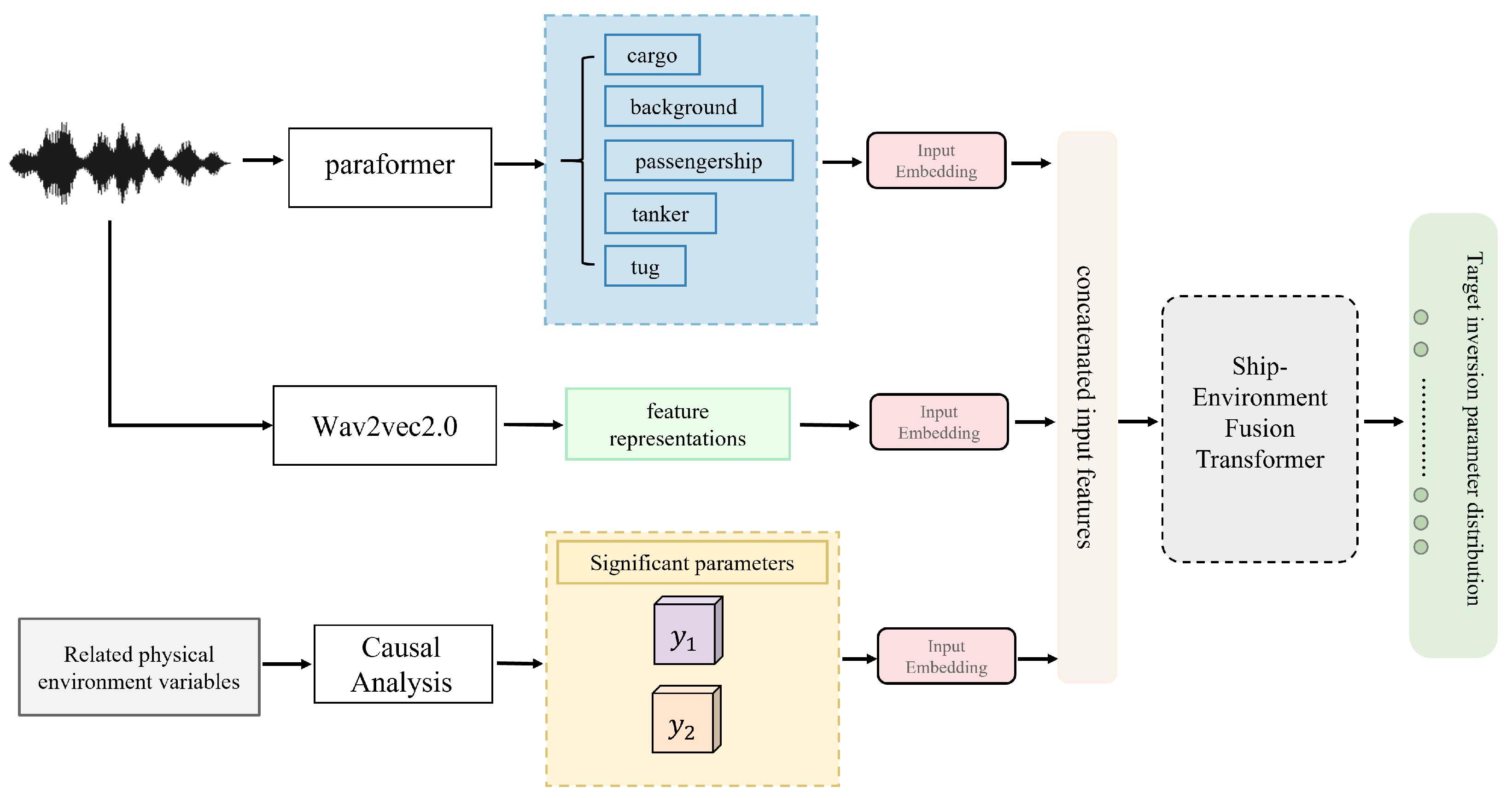
• A causal analysis-driven latent feature fusion network is designed and implemented, integrating source attributes, acoustic data, and causal environmental information, and employing a classification-based strategy instead of regression to achieve high-precision inference of key physical parameters, with GPU acceleration improving inference speed by over sixfold.

The proposed causal modeling deep network framework is experimentally validated on the VTUAD dataset. Experimental results demonstrate significant performance improvements in both seawater temperature and salinity inversion tasks. Furthermore, with GPU acceleration, the inference speed is improved by more than sixfold, fully validating the effectiveness and application potential of the causal analysis-driven latent feature fusion network in complex underwater environments.

Related Works

Ocean Acoustic Tomography, as a non-invasive marine remote sensing technique, has been extensively studied, encompassing traditional optimization methods and emerging deep learning approaches [14]. This section reviews representative works closely related to the present study.

Among traditional methods, Dushaw et al. [1] proposed a single-hydrophone inversion technique based on geometric acoustics models, reconstructing ocean temperature fields by analyzing acoustic propagation times. This method relies on ray tracing algorithms but suffers from high computational complexity, making it suitable for small-scale environments. Martins et al. [3] integrated wavenumber integration with a Bayesian inference framework, developing a more robust parameter inversion approach capable of handling multipath effects. However, its computational cost, on the order of $O\left(N^3\right)$, limits its applicability in large-scale scenarios. Skarsoulis et al. [2] further refined the Bayesian approach by incorporating environmental perturbation modeling, improving inversion stability, though still requiring high-performance computing resources.

In recent years, deep learning has provided new solutions for OAT. Li et al. [7] employed a ConvLSTM model to predict temperature and salinity fields, achieving efficient modeling of spatiotemporal sequences with an accuracy of up to 0.2 °C. However, the method exhibited limitations in complex multipath environments. Wang et al. [8] combined Graph Neural Networks (GNNs) with acoustic tomography techniques to invert temperature fields, significantly reducing computational complexity and enhancing the capability to capture nonlinear relationships, albeit with high sensitivity to input data quality. Sun et al. [9] proposed a deep learning method based on full waveform inversion (FWI), achieving a prediction accuracy of 0.1 °C for temperature and salinity, demonstrating the potential of deep learning for high-precision inversion. Zhang et al. [10] further applied FWI to acoustic tomography in the South China Sea, verifying its applicability in large-scale environments, although the model’s robustness to signal distortion remains to be improved. Vardi and Bonnel [15] proposed an end-to-end geoacoustic inversion method based on deep learning, utilizing a single hydrophone and a 1D Convolutional Neural Network (CNN) to jointly achieve source localization and geoacoustic parameter inversion in shallow water environments. Their method was validated on the Seabed Characterization Experiment 2022 dataset, successfully detecting and localizing 289 Navy SUS (Subsurface Unmanned Signal) explosions with an average localization error of 400 m. The inverted sediment sound speed profiles exhibited spatial variability consistent with traditional methods, while significantly improving computational efficiency.

2. Methodologies

This section introduces three key techniques employed in the causal analysis-driven deep neural network method for marine hydrographic parameter inversion: source target detection via fine-tuning of the Paraformer model, causal analysis, and latent causal feature fusion with its framework.

2.1. Oceanic Hydrological Parameter Inversion

In the ocean acoustic forward problem, we focus on the sound wave propagation process determined by both environmental conditions and sound source characteristics, i.e., how the underwater acoustic signal generated by a specific type of sound source changes as it propagates through a given marine environment and is received by a hydrophone.

Let $\mathbf{e}\in {\mathbb{R}}^m$ represent the ocean environmental variables (such as temperature, salinity, sound speed, etc.), $\mathbf{s}\in {\mathbb{R}}^n$ represent the sound source characteristics (such as sound source type, speed, displacement, etc.), $\mathbf{r}\in {\mathbb{R}}^p$ represent the hydrophone deployment information (such as location, depth, sensor characteristics, etc.), and $\mathbf{a}\in {\mathbb{R}}^d$ represent the acoustic signal features received by the hydrophone (such as spectrum or waveform representation). The generation process of the underwater acoustic signal can be modeled as the following forward mapping:

$$\mathbf{a}=f(\mathbf{e},\mathbf{s},\mathbf{r})+\epsilon ,$$

(1)

where $f(·)$ is a complex nonlinear physical generation function, and $\epsilon$ represents environmental noise and measurement errors.

Therefore, the inverse problem of Ocean Acoustic Tomography, i.e., oceanic hydrological parameter inversion, can be defined as the problem of deducing the ocean environmental variables based on the known acoustic signal features received by the hydrophone, as shown in Equation (2).

$$\mathbf{e}=f^{-1}\left(\mathbf{a}\right).$$

(2)

In this study, based on the definition of the inverse problem, we propose a two-stage inversion strategy to recover the ocean environment state $\mathbf{e}$. Specifically, we first predict the sound source type $\widehat{\mathbf{s}}=f_{\theta }\left(\mathbf{a}\right)$ based on the observed acoustic signal $\mathbf{a}$, and then use the acoustic signal and the predicted result to further estimate the environmental variables $\widehat{\mathbf{e}}=g_{\varphi }(\mathbf{a},\widehat{\mathbf{s}})$.

To describe the two-stage inversion process, we express its goal as minimizing the difference between the predicted environmental parameters and the true environmental parameters, formalized as the following optimization problem:

$$\underset{\theta ,\varphi }{\min }\mathcal{L}\left(g_{\varphi }\left(\mathbf{a},f_{\theta }\left(\mathbf{a}\right)\right),\mathbf{e}\right)$$

(3)

To represent this inversion process more generally and adapt it to broader problems, we generalize it to the following form, representing the inference of unknown states from the observed signals:

$$\widehat{\mathbf{e}}=g_{\varphi }(\mathbf{a},f_{\theta }(\mathbf{a},\mathbf{s}))\approx \arg \underset{\mathbf{e}}{\min }\mathcal{L}\left(\widehat{\mathbf{e}},\mathbf{e}\right)$$

(4)

Here, the function $f_{\theta }(\mathbf{a},\mathbf{s})$ can represent broad sound source features, accepting various types of sound source information as input, such as frequency, intensity, and the position of the sound source. $\mathcal{L}(·)$ is the loss function used to measure the difference between the predicted and true values.

2.2. Source Target Detection via Fine-Tuning of the Paraformer Model

Underwater acoustic environments are characterized by complex and variable signals, low signal-to-noise ratios, and significant redundant information, posing challenges for real-time and high-precision identification of acoustic signals. Non-Autoregressive Automatic Speech Recognition (Non-Autoregressive ASR) models, with their robust parallel decoding capabilities, have been widely adopted in real-time audio processing tasks. The Paraformer (Parallel Autoregressive Transformer) [13], a representative high-performance architecture, introduces a single-step non-autoregressive parallel Transformer framework that maintains recognition accuracy while significantly enhancing inference speed and system throughput. This makes it particularly suitable for acoustic recognition tasks requiring high real-time performance and reliability. The Paraformer’s strong contextual modeling capabilities, adaptive alignment mechanisms, and efficient inference performance render it well-suited for source target identification and hydrographic parameter inversion. In this study, the Paraformer model was fine-tuned on the VTUAD dataset for precise classification of source types, serving as a core component of the multimodal causal analysis network. This architecture provides a stable and scalable foundation for high-quality inversion of critical physical parameters.

As shown in Figure 1, the Paraformer architecture comprises three primary modules. First, the contextual encoding module employs a Transformer-based encoder network to perform deep modeling of input acoustic feature sequences. Through multiple layers of multi-head attention mechanisms and feed-forward networks, this module effectively captures long-range temporal dependencies, yielding high-level acoustic embeddings with global contextual awareness. Second, the Continuous Integrate-and-Fire (CIF) predictor module adaptively predicts the number of output symbols and achieves temporal alignment. The CIF mechanism mimics neural spike firing by integrating acoustic features frame-by-frame, triggering an output when the accumulated value reaches a threshold, thus enabling dynamic alignment between variable-length inputs and outputs. This approach does not rely on strong supervised alignment information, making it inherently suitable for underwater acoustic data, which often exhibits ambiguous annotations and variable-length structures. Finally, the Glancing Language Model (GLM) incorporates partial ground-truth target labels as prior information during training, guiding the network to learn contextual dependencies among targets. This strategy effectively mitigates the exposure bias issue common in non-autoregressive models, significantly enhancing semantic modeling capabilities and final recognition accuracy.

The Paraformer model offers several advantages for source type identification tasks. First, its adaptive temporal alignment, facilitated by the CIF module, eliminates the need for precise alignment annotations, making it particularly suitable for underwater acoustic signals with inherent alignment uncertainties. Second, its efficient parallel processing and low-latency characteristics, derived from the non-autoregressive decoding framework, substantially reduce inference time, meeting the real-time requirements of marine acoustic monitoring applications. Additionally, the joint contextual and semantic modeling capabilities, achieved through the synergy of the encoder and GLM, enable the model to accurately capture subtle yet discriminative patterns in acoustic features across different sources.

2.3. Causal Analysis

The inversion of ocean hydrographic parameters involves multiple observational variables. Directly using raw observational variables as model inputs can introduce redundant features or confound causal directions, leading to reduced generalization performance of inversion models. To address this, causal inference methods are employed to identify and select key factors with significant impacts on target inversion variables. Specifically, this study adopts Causal Representation Learning to construct causal graphs among variables, followed by intervention estimation models (e.g., double distribution regressors or causal forests) to quantify the causal contributions of environmental variables to inversion outcomes. Based on this, a subset of physically driven features is extracted for embedding modeling and integrated into a multimodal network to enhance the synergistic inference capabilities for source target identification and physical parameter inversion.

Causal inference extends beyond data-driven correlation modeling to mechanistic causal modeling, emphasizing causal effects under hypothetical interventions. This is particularly significant for modeling dependencies among physical quantities in complex marine environments. The theoretical foundation of causal analysis relies on two primary paradigms: the structural causal model (SCM) and the potential outcome framework. The SCM explicitly defines dependency paths and information flow mechanisms among variables through causal graphs, enabling the computation of causal effects using do-calculus. The potential outcome framework, on the other hand, focuses on comparing potential outcome differences between intervention and non-intervention scenarios under controlled covariates, estimating the average treatment effect (ATE) of treatment variables. Consider an observational dataset,

$$D={\left\{(x_i,y_i)\right\}}_{i=1}^n,$$

where $x=(t,w)\in {\mathbb{R}}^d$ comprises a binary treatment variable $t\in \{0, 1\}$ and covariates $w\in {\mathbb{R}}^{d-1}$, and $y\in \mathbb{R}$ represents the outcome variable. The ATE of the treatment variable t on the outcome y is defined as

$$\mathrm{ATE}=\mathbb{E}[y\mid \mathrm{do}(t=1\left)\right]-\mathbb{E}[y\mid \mathrm{do}(t=0\left)\right],$$

where $\mathrm{do}(·)$ denotes an external intervention operation. Unlike traditional correlation analysis, the do-operation evaluates true causal effects by “severing” dependencies between a variable and its parent nodes, aligning with the interpretative needs of physical mechanisms.

2.4. Latent Causal Feature Fusion and Framework

Latent causal feature fusion has garnered significant attention in complex environmental perception and high-dimensional data modeling tasks. Its core objective is to integrate latent feature embeddings generated through causal inference within a unified learning framework. These embeddings are derived from diverse information sources (e.g., acoustic features, environmental variables, and source attributes), enhancing the model’s expressive power, discriminative capability, and generalization performance. Compared to traditional models relying on single modalities, latent causal feature fusion captures complementary and causal relationships among different information sources, thereby improving robustness and performance in scenarios with high uncertainty and complex data dimensions.

The intrinsic characteristics of ocean hydrographic parameter inversion are often distributed across multiple information sources. For instance, acoustic features capture spectral characteristics of sound propagation underwater, serving as critical direct information for source-type identification. Source prior attributes (e.g., vessel tonnage, speed, and structural classification) reflect prior structural constraints on source and propagation characteristics. Environmental variables (e.g., seawater temperature, depth, salinity, and water column stratification) significantly influence sound wave propagation paths and attenuation, constituting essential perturbation factors in physical parameter inversion modeling. Traditional hydrographic parameter inversion methods often rely on single information sources (e.g., acoustic spectrograms), overlooking the coupling mechanisms and causal influences among different sources, which hinders accurate modeling of signal variations in complex environments. To address this, a latent causal feature fusion strategy is introduced, where acoustic features, environmental variables, and source attributes are transformed into structured latent causal feature embeddings through causal inference. These embeddings are then uniformly encoded into a latent causal feature fusion network to enable synergistic modeling for ocean hydrographic parameter inversion tasks.

3. Neural Networks

To address practical challenges in marine environments, such as high acoustic signal noise and signal distortion, a deep neural network framework is proposed for ocean hydrographic parameter inversion. This framework integrates speech classification, acoustic feature modeling, and causality-driven physical embedding information to enhance model robustness and interpretability.

The overall workflow of the system is illustrated in Figure 2, comprising three core components: a source target identification module, an acoustic feature modeling module, and a multimodal fusion module driven by physical embeddings. First, advanced speech modeling networks process raw audio data collected by hydrophones to generate high-confidence classification labels representing acoustic source features. Second, self-supervised learning is employed to extract stable and robust temporal representations from audio signals, capturing complex acoustic patterns in marine sound propagation. Third, key environmental physical parameters are selected based on causal analysis and encoded into structured embedding information, enhancing the system’s ability to model environmental variations. Finally, the extracted information is fused in the embedding space and input into a unified neural network architecture for joint optimization, achieving hydrographic parameter inversion based on source target identification. To further improve model generalization and interpretability, certain regression tasks are transformed into discrete classification problems, reducing training complexity and enhancing inference accuracy.

3.1. Ocean Hydrographic Parameter Inversion

To incorporate physically meaningful embeddings into the multimodal learning framework, causal analysis is conducted to identify key environmental variables influencing the target inversion parameters (e.g., temperature).

Causal inference is based on the structural causal model (SCM) and the potential outcome framework [16]. Given an observational dataset

$$D={\left\{(x_i,y_i)\right\}}_{i=1}^n,$$

(5)

where $x=(t,w)\in {\mathbb{R}}^d$ comprises a binary treatment variable $t\in \{0, 1\}$ and other covariates $w\in {\mathbb{R}}^{d-1}$, and $y\in \mathbb{R}$ represents the outcome variable. The average treatment effect (ATE) of the treatment t on the outcome y is defined as

$$\mathrm{ATE}=\mathbb{E}\left[y\mid \mathrm{do}(t=1)\right]-\mathbb{E}\left[y\mid \mathrm{do}(t=0)\right],$$

(6)

where $\mathrm{do}(·)$ denotes an intervention operation that fixes t to a specified value and severs its dependencies with parent nodes in the causal graph.

A directed acyclic graph (DAG) is constructed based on domain knowledge to model causal relationships among environmental variables. The graph includes nodes for temperature, salinity, sound speed, pressure, conductivity, duration, sampling rate, and source type. Taking temperature as the target inversion parameter, it is assumed that salinity, sound speed, pressure, and conductivity directly affect temperature; duration and sampling rate influence all environmental variables; and source type causally impacts all physical parameters, as shown in Figure 3. Based on this graph, the backdoor criterion is applied to select an adjustment set $Z\subseteq \{w_1,w_2,\dots ,w_{d-1}\}$ that blocks all backdoor paths from t to y without including descendants of t, thereby eliminating confounding bias. When the backdoor criterion is satisfied and the causal effect is identifiable, the intervention distribution is estimated as follows:

$$p(y\mid \mathrm{do}(t))=\int p(y\mid t,Z)p(Z)dZ.$$

(7)

The implementation of causal inference relies on the DoWhy library [17]. Salinity, sound speed, pressure, and conductivity are treated as treatment variables, with temperature and other physical quantities as outcome variables. For each treatment–outcome pair, a CausalModel is constructed, the backdoor criterion is applied to identify the adjustment set, and linear regression is used to estimate the ATE. Additionally, sensitivity analysis is conducted using the random common cause method to evaluate the robustness of estimates against unobserved confounders.

The entire causal analysis process is outlined in Algorithm 1. Ultimately, based on the absolute ATE values, the environmental parameters with the most significant causal impacts are selected to construct physical information embeddings, thereby enhancing the model’s physical interpretability.

Algorithm 1 Causal Analysis of Environmental Parameters

Require: Observational dataset $D={\left\{(x_i,y_i)\right\}}_{i=1}^n$, causal graph $\mathcal{G}$, treatment variable set $\mathcal{T}$, outcome variable set $\mathcal{Y}$ Ensure: Causal graph visualization, ATE estimates, key feature set   1: Initialize the causal graph $\mathcal{G}$ based on marine domain knowledge   2: for each treatment variable $t\in \mathcal{T}$ do   3:  for each outcome variable $y\in \mathcal{Y}$ do   4:   Construct a CausalModel, setting t as treatment and y as outcome   5:   Apply the backdoor criterion to identify the adjustment set Z   6:   Estimate the intervention distribution $p(y\mid \mathrm{do}(t\left)\right)$ using linear regression   7:   Compute ATE: $\mathbb{E}\left[y\right|\mathrm{do}(t=1)]-\mathbb{E}[y\left|\mathrm{do}\right(t=0\left)\right]$   8:   Perform sensitivity analysis using the random common cause method   9:  end for  10: end for  11: Select the top k key features for each outcome variable based on $\left|\mathrm{ATE}\right|$ magnitude  12: return Causal graph $\mathcal{G}$, ATE values, selected features

3.2. Latent Causal Feature Fusion and Joint Modeling

3.2.1. Physically-Informed Embedding Generation

Following source target classification, physically-informed embeddings are constructed by integrating source type information, environmental variables, and acoustic features to address the challenges posed by complex hydrodynamic and acoustic interactions in marine environments for physical parameter inversion. These embeddings comprise three components: environmental parameters selected through causal analysis, categorical embeddings of source types, and audio features extracted using wav2vec 2.0 [18].

Initially, wav2vec 2.0 is pre-trained on raw speech signals. The input waveform ${\mathbf{x}}_{\mathrm{wav}}$ is processed by a multi-layer convolutional feature encoder:

$${\mathbf{z}}_t=f_{\mathrm{enc}}\left({\mathbf{x}}_{\mathrm{wav}}\right)\in {\mathbb{R}}^d,$$

(8)

where p time steps of continuous segments of length M are randomly masked and replaced with learned mask vectors, yielding a masked latent sequence $\tilde{\mathbf{z}}$ [18]. Subsequently, $\tilde{\mathbf{z}}$ is fed into a multi-layer Transformer context network g, producing contextualized representations:

$${\mathbf{c}}_t=g\left(\tilde{\mathbf{z}}\right)\in {\mathbb{R}}^{d_a},$$

(9)

where $d_a=768$. A quantization module Q discretizes ${\mathbf{z}}_t$ into ${\mathbf{q}}_t=Q\left({\mathbf{z}}_t\right)$ using G codebooks. During pre-training, a contrastive loss is applied at each masked position t:

$${\mathcal{L}}_{\mathrm{contra}}=-\sum _t\log {\displaystyle \frac{\exp \left(\mathrm{sim}({\mathbf{c}}_t,{\mathbf{q}}_t)/\kappa \right)}{{\sum }_{\tilde{\mathbf{q}}\in {\mathcal{Q}}_t}\exp \left(\mathrm{sim}({\mathbf{c}}_t,\tilde{\mathbf{q}})/\kappa \right)}},$$

(10)

where ${\mathcal{Q}}_t$ includes the true code ${\mathbf{q}}_t$ and K distractor samples, $\mathrm{sim}(\mathbf{u},\mathbf{v})={\mathbf{u}}^{\top }\mathbf{v}/\parallel \mathbf{u}\parallel \parallel \mathbf{v}\parallel$ denotes cosine similarity, and $\kappa$ is a temperature parameter [18]. A diversity loss is also applied to encourage uniform codebook usage. After pre-training, the Transformer context outputs $\left\{{\mathbf{c}}_t\right\}$ form the final audio features:

$${\mathbf{f}}_{\mathrm{audio}}=[{\mathbf{c}}_1,\dots ,{\mathbf{c}}_L]\in {\mathbb{R}}^{L\times d_a},$$

(11)

where L is the sequence length and $d_a=768$ is the hidden dimension, effectively capturing key acoustic patterns in marine sound propagation.

Subsequently, two types of embeddings are defined:

$${\mathbf{e}}_{\mathrm{ship}}=f_{\mathrm{ship}}(t_{\mathrm{ship}};{\theta }_s),{\mathbf{e}}_{\mathrm{env}}=f_{\mathrm{env}}(S,C;{\theta }_e),$$

(12)

where $t_{\mathrm{ship}}$ is the categorical index of the source type, and $f_{\mathrm{ship}}$ is an embedding layer mapping source types to a 64-dimensional space; S and C represent environmental features such as salinity and conductivity, and $f_{\mathrm{env}}$ is a transformation that linearly maps these two-dimensional environmental variables to a 256-dimensional shared space. Both source type and environmental embeddings are then mapped to a common $d=256$-dimensional space via linear transformations to achieve multimodal feature alignment. Source embeddings implicitly learn and reflect hydrodynamic constraints (e.g., drag and wave effects due to source size and speed), while environmental embeddings encode key physical parameters affecting sound speed propagation (e.g., the influence of salinity on sound speed) [19]. The selection of environmental variables is guided by the causal analysis results from Section 2.3, prioritizing variables with the highest average treatment effects to enhance physical interpretability and reduce noise interference.

This approach leverages causal relationships and observational data, including audio, source target classification, and environmental parameters, to capture marine physical information, enabling robust feature representations for ocean hydrographic parameter inversion. It is particularly effective in noisy underwater scenarios, providing a reliable foundation for subsequent physical parameter classification and inversion tasks.

3.2.2. Multimodal Fusion Network Architecture

Based on the physically-informed embeddings proposed in Section 3.2.1, a cascaded processing pipeline is constructed to integrate audio, source features, and environmental variables for physical parameter inversion in marine environments. Initially, audio signals are input into the Paraformer speech recognition model, which undergoes full-parameter fine-tuning to optimize the pre-trained model by unfreezing and updating all parameters. Compared to lightweight fine-tuning methods (e.g., LoRA), full-parameter fine-tuning fully activates the model’s representation capabilities, effectively adapting to the complex characteristics of multimodal marine inversion tasks. During training, mixed-precision and distributed training techniques are employed to ensure efficient and stable model optimization. The fine-tuning process adjusts batch sizes dynamically based on audio–text pairs and token counts from the VTUAD dataset, achieving efficient parameter updates, reduced computational overhead, and rapid convergence. The fine-tuned Paraformer outputs vessel type classification labels, serving as one of the initial input modalities.

Subsequently, the wav2vec 2.0 model [18] is used to extract feature representations from audio signals, capturing complex acoustic patterns critical to marine sound propagation. These audio features, along with vessel type embeddings generated by Paraformer and environmental features (e.g., salinity and conductivity) selected through causal analysis in Section 2.3, are used to construct physically-informed embeddings ${\mathbf{e}}_{\mathrm{audio}}$, ${\mathbf{e}}_{\mathrm{ship}}$, and ${\mathbf{e}}_{\mathrm{env}}$. These embeddings are projected into a common 256-dimensional space via linear transformations:

$${\mathbf{h}}_{\mathrm{audio}}=f_{\mathrm{audio}}({\mathbf{e}}_{\mathrm{audio}};{\theta }_a),{\mathbf{h}}_{\mathrm{ship}}=f_{\mathrm{ship}}({\mathbf{e}}_{\mathrm{ship}};{\theta }_s),{\mathbf{h}}_{\mathrm{env}}=f_{\mathrm{env}}({\mathbf{e}}_{\mathrm{env}};{\theta }_e).$$

(13)

Here, ${\mathbf{e}}_{\mathrm{audio}}$ is derived from the wav2vec 2.0 output, ${\mathbf{e}}_{\mathrm{ship}}$ encodes the vessel type index, and ${\mathbf{e}}_{\mathrm{env}}$ aggregates physical variables identified through causal analysis.

Next, the three feature streams are concatenated along the sequence dimension and processed through a multi-head attention (MHA) mechanism to enhance cross-modal interactions. Drawing on successful experiences in capturing global dependencies in multimodal data [20,21], an MHA mechanism with eight heads is applied prior to feature fusion. This mechanism projects inputs into query (Q), key (K), and value (V) matrices, enabling the model to adaptively focus on critical information across modalities and sequence positions. For the i-th attention head, the computation is as follows:

$$\mathrm{Attention}(Q_i,K_i,V_i)=\mathrm{softmax}\left({\displaystyle \frac{Q_i{K}_i^{\top }}{\sqrt{d_k}}}\right)V_i,$$

(14)

where

$$Q_i={\mathbf{h}}_{\mathrm{concat}}{W}_i^Q,K_i={\mathbf{h}}_{\mathrm{concat}}{W}_i^K,V_i={\mathbf{h}}_{\mathrm{concat}}{W}_i^V,$$

(15)

and $W_i^Q,W_i^K,W_i^V\in {\mathbb{R}}^{d\times d_k}$ are trainable projection matrices, with $d_k=d/\mathrm{num}\_\mathrm{heads}=256/8=32$. The outputs of all heads are concatenated and linearly mapped:

$${\mathbf{h}}_{\mathrm{attended}}=\mathrm{Concat}({\mathrm{head}}_1,\dots ,{\mathrm{head}}_8)W^O,$$

(16)

where $W^O\in {\mathbb{R}}^{d\times d}$, resulting in ${\mathbf{h}}_{\mathrm{attended}}\in {\mathbb{R}}^{L\times d}$.

The ${\mathbf{h}}_{\mathrm{attended}}$ is then fed into a Transformer encoder with four layers, each with eight heads and a dropout rate of 0.1, to further refine the fused features. Each layer consists of a multi-head self-attention sublayer and a feed-forward network (FFN) sublayer, both employing residual connections and layer normalization (LN). To preserve sequence positional information, positional encoding is added before input:

$$P{E}_{(pos,2i)}=\sin \left({\displaystyle \frac{pos}{{10000}^{2i/d}}}\right),P{E}_{(pos,2i+1)}=\cos \left({\displaystyle \frac{pos}{{10000}^{2i/d}}}\right),$$

(17)

yielding

$${\mathbf{x}}_0={\mathbf{h}}_{\mathrm{attended}}+PE.$$

(18)

The computation for the ℓ-th layer ($\ell =1,\dots ,4$) is:

$$\begin{array}{cc}\hfill {\mathbf{x}}_{\ell }^{\prime }& =\mathrm{LN}\left(\mathrm{MHSA}\left({\mathbf{x}}_{\ell -1}\right)+{\mathbf{x}}_{\ell -1}\right),\hfill \end{array}$$

(19)

$$\begin{array}{cc}\hfill {\mathbf{x}}_{\ell }& =\mathrm{LN}\left(\mathrm{FFN}\left({\mathbf{x}}_{\ell }^{\prime }\right)+{\mathbf{x}}_{\ell }^{\prime }\right),\hfill \end{array}$$

(20)

where the FFN is defined as:

$$\mathrm{FFN}\left(\mathbf{x}\right)=\mathrm{ReLU}(\mathbf{x}{W}_1+b_1)W_2+b_2,$$

(21)

with $W_1\in {\mathbb{R}}^{d\times d_{\mathrm{ff}}}$, $W_2\in {\mathbb{R}}^{d_{\mathrm{ff}}\times d}$, and $d_{\mathrm{ff}}=1024$. The encoder’s final output is ${\mathbf{h}}_{\mathrm{fused}}={\mathbf{x}}_4$, capturing both local and global dependencies [21].

The architecture of the Ship Environment Fusion Transformer is illustrated in Figure 4. This figure depicts the feature fusion stage within the complete multimodal inversion pipeline shown in Figure 2, specifically highlighting the cross-modal interactions of vessel type embeddings, environmental feature embeddings, and audio features via the multi-head attention mechanism, as well as the feature refinement process through the Transformer encoder.

The last token representation of the Transformer output sequence is extracted, passed through a dropout layer (rate 0.3), and fed into a linear layer for prediction. In traditional physical parameter inversion tasks, regression is commonly used to directly model target variables (e.g., seawater temperature or salinity). While regression methods achieve high numerical accuracy in certain domains, such as environmental sensor value prediction or meteorological parameter estimation, they often struggle to provide stable and high-resolution outputs in applications with multimodal inputs, significant observational noise, and complex relationships between features and targets. In marine environments, sound propagation is influenced by multiple coupled factors (e.g., salinity, temperature, depth, and vessel interference), and even if regression models produce outputs close to true values overall, accumulated errors from nonlinear mappings can lead to estimation biases in localized regions. Such errors are particularly sensitive in certain physical metrics, ultimately reducing inversion accuracy, especially for high-resolution monitoring tasks.

To address these challenges, this study leverages the advantages of classification in high-resolution tasks by reformulating continuous-value inversion as a multi-class classification problem. The numerical range of each target physical quantity is uniformly discretized into multiple intervals (e.g., 100 or 1000 intervals based on precision requirements), with each interval corresponding to a class label. This transforms the model’s learning objective into determining the interval in which the input sample’s physical quantity lies, mitigating accumulated errors and distribution shifts associated with direct continuous value prediction.

Compared to regression methods, which typically rely on loss functions such as MSE or MAE, the classification strategy with cross-entropy loss (CrossEntropyLoss) imposes clearer penalties on errors during training and is more sensitive to boundaries, enabling the model to focus on fine-grained discrimination near interval boundaries. This enhances the robustness and discriminability of physical parameter estimation. During inference, the predicted class label is mapped back to the midpoint of the corresponding interval to obtain the numerical estimate.

To convert the continuous-value inversion problem into a classification task, the target physical quantity (e.g., temperature) is uniformly discretized into 1000 intervals within its expected range. Given a true value y, its class label c is computed as:

$$c=\mathrm{floor}\left({\displaystyle \frac{y-y_{\min }}{y_{\max }-y_{\min }}}\times 1000\right),$$

(22)

where $y_{\min }$ and $y_{\max }$ are the lower and upper bounds of the parameter range, respectively. During inference, the predicted class is mapped to the midpoint of the corresponding interval. This discretization approach simplifies the continuous optimization problem into a classification task, leveraging classification strategies to enhance robustness to marine environmental noise. In summary, by reformulating the physical inversion problem as a classification task and integrating multimodal representations with deep attention mechanisms, the proposed approach better adapts to high-resolution inversion demands in complex environments, providing a stable foundation for subsequent physical inference and downstream analysis.

4. Experimental Configuration

This section provides a detailed description of the dataset used in this study, the loss function design employed during model training, and the specific experimental setup. These elements collectively form the foundation for model evaluation and comparative experiments, ensuring the reproducibility and scientific rigor of the research results.

4.1. Dataset Description

This study employs the VTUAD dataset for experimental validation. The dataset is a curated collection of underwater acoustic data sourced from the Ocean Networks Canada initiative, collected between 24 June and 3 November 2017, in the Georgia Strait, Canada. It represents typical operational scenarios during the pre-pandemic summer and autumn seasons. Acoustic signals were captured using an icListen AF hydrophone deployed 147 m below sea level, supplemented by Automatic Identification System (AIS) data for vessel positioning. Environmental data were recorded using a Sea-Bird SBE 16plus SEACAT recorder(Sea-Bird Scientific, Bellevue, WA, USA), a high-precision CTD instrument designed for fixed deployments.

The VTUAD dataset includes five categories of underwater acoustic signals: cargo, tanker, tug, passengership, and background. The data are divided into three subsets (or scenarios) based on the distance between vessels and the hydrophone: Scenario 1 (within a 2 km radius, excluding 3 km, i.e., distances between 2 and 3 km); Scenario 2 (within a 3 km radius, excluding 4 km, i.e., distances between 3 and 4 km); and Scenario 3 (within a 4 km radius, excluding 6 km, i.e., distances between 4 and 6 km). Additionally, the dataset provides environmental information, including mean values for five parameters: temperature (in degrees Celsius), conductivity (in Siemens per meter), pressure (in decibars), salinity (in Practical Salinity Units, PSU), and sound speed (in meters per second).

The dataset’s strength lies in its real marine environmental data, the diversity of sound sources (i.e., ship types), and the inclusion of environmental information, making it suitable for hydrological parameter inversion tasks. However, the dataset has certain limitations, such as some audio files potentially being corrupted or containing noise, and the data distribution across different distance scenarios may not be balanced. Additionally, we filtered the dataset to ensure all samples contain complete environmental metadata, thus eliminating missing values in the environmental parameters that are critical for our analysis. In this study, we primarily used the data from Scenario 1 for the experiments to ensure data quality, and we enhanced model training stability through data cleaning and preprocessing. Scenario 1 contains approximately 20,000 samples, with around 7000 samples per category (cargo ships, tankers, tugboats, passenger ships, and background). The dataset creators have pre-split the data into training and testing sets. To improve the model’s generalizability, we re-adjusted the dataset while maintaining the original training-testing ratio, ensuring approximately 7000 training samples and 300 testing samples per category. This re-adjustment ensures balanced representation of each category, mitigating potential biases in the original split.

The VTUAD dataset was chosen because it has unique advantages in the field of Ocean Acoustic Tomography (OAT) compared to other datasets. Unlike the ShipsEar dataset [22], which contains only around 100 samples, the VTUAD dataset provides a larger sample size that meets the data requirements for deep learning methods. Similarly, although the DeepShip dataset [23] is larger, it lacks the comprehensive environmental metadata required for our study, such as temperature, salinity, and sound speed.

4.2. Loss Functions

Model training in this study is divided into two stages, each with distinct loss functions tailored to the tasks of speech classification pre-training and physical parameter inversion via latent causal feature fusion.

For the source target identification task, the Paraformer speech recognition model is fine-tuned within the FunASR framework to extract structured semantic information from acoustic signals. This stage employs FunASR’s default joint loss mechanism, combining Connectionist Temporal Classification (CTC) loss, ${\mathcal{L}}_{\mathrm{ctc}}$, with sequence-to-sequence cross-entropy loss, ${\mathcal{L}}_{\mathrm{ce}}$, to achieve multi-level alignment optimization between acoustic sequences and semantic labels. The overall loss function is defined as:

$${\mathcal{L}}_{\mathrm{paraformer}}={\lambda }_{\mathrm{ctc}}·{\mathcal{L}}_{\mathrm{ctc}}+(1-{\lambda }_{\mathrm{ctc}})·{\mathcal{L}}_{\mathrm{ce}},$$

(23)

where the hyperparameter ${\lambda }_{\mathrm{ctc}}\in [0, 1]$ controls the weighting of the two sub-objectives. This combined loss function significantly enhances consistency in sequence modeling and target classification, improving the model’s ability to discriminate source types in complex acoustic scenarios.

For the final physical parameter inversion task, continuous hydrographic variables (e.g., temperature) are discretized into multiple intervals, transforming the problem into a multi-class classification task. The cross-entropy loss function is used as the primary optimization objective, expressed as:

$${\mathcal{L}}_{\mathrm{ce}}=-\sum _{i=1}^C{y}_i\log \left({\widehat{y}}_i\right),$$

(24)

where C denotes the number of discrete classes, $y_i$ is the one-hot representation of the true class, and ${\widehat{y}}_i$ is the model’s softmax probability output. The cross-entropy loss effectively improves classification accuracy and adapts to the complex noise conditions of marine environments, enhancing the robustness of inversion results.

4.3. Experimental Setup

The hardware environment for the experiments is detailed in

Table 1. Experimental hardware environment.

CPU	Intel(R) Xeon(R) Gold 6230 CPU @ 2.10 GHz (Santa Clara, CA, USA)
OS	Ubuntu 20.04 LTS
GPU	NVIDIA Tesla V100-SXM2-32 GB (Santa Clara, CA, USA)
CUDA Version	CUDA 12.6

. The software environment is based on Python 3.9.21, with model implementation using the PyTorch 2.5.1 framework. Training is conducted for 100 epochs, with a batch size of 32 samples per iteration for weight updates. The AdamW optimizer is employed with an initial learning rate of 0.0001, and a cosine annealing strategy is used to dynamically adjust the learning rate. The model parameter settings are summarized in

Table 2. Experimental parameter settings.

Model Layers	Dropout	Epochs	Learning Rate Strategy
4	0.3	100	Cosine Annealing
Batch Size	Initial Learning Rate	Optimizer
32	0.0001	AdamW

.

In the experiments, the VTUAD dataset is split into training and test sets with a ratio of 19:1 (36,510 training samples and 1880 test samples).

5. Results

Experiment of Model

To further validate the model’s performance in hydrographic parameter inversion tasks, experiments were conducted on Scenario 1 data from the VTUAD dataset, focusing on the discretized prediction of temperature and salinity. Taking temperature as an example inversion target, the temperature values were discretized into 1000 classes, and the model’s performance was evaluated on the validation set. The model achieved an accuracy of 98.68% on the validation set, demonstrating strong robustness for temperature inversion in complex marine environments. To provide deeper insights into the model’s predictive behavior, various visualization methods were employed to present and analyze the experimental results. Additionally, we evaluated several performance metrics, including accuracy, F1 score, precision, recall, and area under the curve (AUC).

The confusion matrices (Figure 5) indicate that the model effectively distinguishes between different temperature classes, with most misclassifications occurring between adjacent classes, reflecting the smooth nature of temperature predictions. The class distribution plot (Figure 6) compares the true and predicted temperature distributions on the validation set, covering the first 50 classes. The temperature range spans 1000 classes from 9.15 °C to 10.55 °C, with an interval of 0.0014 °C per class. Among the 1000 classes, the validation set covers 191 classes. With 1000-class discretization, higher classification precision is achieved. For 100-class discretization, the temperature distribution is relatively balanced, as shown in Figure 6, though sample counts vary across classes, and prediction accuracy is slightly lower compared to 1000-class discretization.

To intuitively assess the model’s predictive performance, Figure 7 illustrates the temperature inversion results of the latent causal feature fusion network on the validation set, comparing the probability density distributions of true and predicted temperature values. This plot is generated using kernel density estimation (KDE), with the x-axis representing temperature values (ranging from 9.15 °C to 10.55 °C) and the y-axis indicating probability density. The blue solid line represents the true temperature distribution, while the orange dashed line represents the predicted temperature distribution. The two curves exhibit high alignment in shape and position, with only a slight underestimation in the high-temperature region (above 10.4 °C), indicating the model’s ability to effectively capture temperature distribution characteristics.

The accuracy curve (Figure 8) depicts the accuracy variation across training epochs for 100-class temperature discretization, with a final validation accuracy of 98.61%. For 1000-class discretization, the final validation accuracy is 97.77%.

In addition to temperature, experiments were conducted on salinity as an inversion target, comparing the probability density distributions of predicted and true salinity values. Based on causal analysis, the most relevant environmental variables for salinity were conductivity and sound speed. Similar to the temperature setup, salinity was discretized into 100 classes, ranging from 30.15 PSU to 30.75 PSU, with an interval of 0.006 PSU per class. The model achieved a validation accuracy of 96.38% for salinity prediction, demonstrating its effectiveness in handling multiple hydrographic parameters.

To further evaluate the model’s performance in salinity inversion, Figure 9 presents the probability density distributions of true and predicted salinity on the validation set, also generated using KDE. The x-axis represents salinity values, and the y-axis indicates probability density. The blue solid line represents the true salinity distribution, while the orange dashed line represents the predicted salinity distribution. The two curves show high consistency, indicating that the latent causal feature fusion network effectively captures salinity distribution characteristics.

To comprehensively demonstrate the model’s performance in the temperature and salinity inversion tasks, we summarize the results on the validation set in

Table 3. Experimental results for temperature and salinity inversion tasks.

Inversion Parameter	Classes	Accuracy (%)	F1 Score	Recall (%)	Precision (%)	AUC
Temperature	100	98.61	0.985	96.95	97.26	0.99
	1000	97.77	0.978	96.08	96.59	0.99
Salinity	100	96.72	0.964	96.28	96.28	0.99
	1000	95.52	0.955	94.54	94.86	0.99

, including accuracy, F1 score, recall, precision, and AUC. Accuracy is defined as the ratio of correctly classified samples to the total number of samples, and is calculated as follows:

$$\mathrm{Accuracy}={\displaystyle \frac{\mathrm{TP}+\mathrm{TN}}{\mathrm{TP}+\mathrm{TN}+\mathrm{FP}+\mathrm{FN}}}\times 100\%$$

(25)

where TP (true positive) is the number of true positive samples, TN (true negative) is the number of true negative samples, FP (false positive) is the number of false positive samples, and FN (false negative) is the number of false negative samples. The F1 score is the harmonic mean of precision and recall, calculated as:

$$\mathrm{F}1\mathrm{Score}=2\times {\displaystyle \frac{\mathrm{Precision}\times \mathrm{Recall}}{\mathrm{Precision}+\mathrm{Recall}}}$$

(26)

Here, $\mathrm{Precision}={\displaystyle \frac{\mathrm{TP}}{\mathrm{TP}+\mathrm{FP}}}$ represents precision, and $\mathrm{Recall}={\displaystyle \frac{\mathrm{TP}}{\mathrm{TP}+\mathrm{FN}}}$ represents recall. Accuracy reflects the overall correctness of the model’s classification, while the F1 score considers both precision and recall, making it particularly suitable for evaluating performance under class imbalance in multi-class classification tasks. In addition, the AUC (area under the ROC curve) metric is used to assess the overall ability of the model to distinguish between positive and negative samples. The ROC curve depicts the relationship between the false positive rate (FPR) and true positive rate (TPR) under varying thresholds. An AUC value closer to 1 indicates better classification performance, whereas an AUC near 0.5 suggests that the model performs no better than random guessing. AUC is especially useful for evaluating the robustness of models under multi-class or imbalanced data conditions.

Table 3 presents the overall performance of the latent causal feature fusion network in the temperature and salinity inversion tasks. Under the 100-class setting, the inversion accuracy for temperature and salinity reached 98.61% and 96.72%, respectively. The F1 scores also remained at high levels (0.985 and 0.964, respectively), with both recall and precision exceeding 96%, indicating that the model possesses strong discriminative ability and stable predictive performance in medium-granularity classification tasks.

As the number of classes increases to 1000, the inversion task becomes significantly more challenging. Under this setting, the inversion accuracy for temperature and salinity drops to 97.77% and 95.52%, respectively. However, the F1 scores remain above 0.955, and the decreases in recall and precision are relatively small, indicating that the model still maintains a good classification balance when handling high-resolution classification tasks.

In terms of the AUC metric, all tasks maintain an AUC of 0.99 under both the 100-class and 1000-class settings, indicating that the model exhibits stable discriminative capability across different classification thresholds. This is particularly valuable for handling imbalanced class distributions or evaluating probabilistic outputs. These results suggest that the model not only achieves accurate classification but also effectively ranks prediction probabilities, making it well-suited for fine-grained hydrological parameter inversion in complex marine environments.

Further observations from the confusion matrix shown in Figure 5 reveal that most classification errors are concentrated between adjacent classes with similar temperature values. This indicates that the model exhibits a certain degree of uncertainty when distinguishing within boundary regions of temperature. Such local errors may be attributed to the physical continuity of temperature itself—since real-world temperature distributions are typically smooth in space, discretization labeling may introduce artificial “hard boundaries” leading to deviations between the predicted classes and the true labels.

In terms of probability density distribution, Figure 7 and Figure 9 illustrate the kernel density estimation (KDE) comparison between the model predictions and the ground truth. The results show a high degree of consistency between the two, with only slight deviations observed in the high-temperature range (>10.4 °C) and mid-to-high salinity intervals. These deviations may result from the relative sparsity of training samples in high-value regions or from nonlinear disturbances caused by local environmental variations (e.g., small-scale mixing, seabed topography, and other unmodeled factors). Overall, the model demonstrates high reliability in capturing the distribution of temperature and salinity across the major value ranges.

It is worth noting that the overall performance of temperature inversion is superior to that of salinity prediction. This may be attributed to the relatively stable spatiotemporal variation of temperature, whereas salinity is influenced by a combination of factors such as ocean currents, precipitation, evaporation, and estuarine mixing, resulting in a more complex spatial distribution and greater prediction difficulty. Future work may consider incorporating additional physical variables (e.g., wind stress, sea surface evaporation, and bathymetric information) to enhance the model’s ability to capture the underlying mechanisms of salinity variation.

In summary, the experimental results demonstrate that the proposed latent causal feature fusion network exhibits strong predictive performance and robustness across multi-granularity and multi-parameter oceanic hydrological inversion tasks, indicating its promising generalization ability and practical application value.

Inference Speed Comparison Experiment

To evaluate the performance of the latent causal feature fusion network under hardware acceleration, the inference speeds of the model on GPU and CPU were compared. Experiments were conducted on the validation set of the VTUAD dataset, measuring the single-pass inference times for temperature and salinity inversion tasks. The hardware environment consisted of a CPU (Intel(R) Xeon(R) Gold 6230 @ 2.10 GHz, 20 cores) and a GPU (NVIDIA Tesla V100-SXM2-32 GB, 32 GB HBM2, 1410 MHz). Model parallelization was implemented using PyTorch’s DataParallel module, leveraging the GPU’s multi-core parallel computing capabilities.

Table 4. Model inference costs.

Inversion Parameter	CPU (Seconds)		GPU (Seconds)
	Average Time	Speedup Ratio	Average Time	Speedup Ratio
Temperature	37.49	1.00	5.73	6.54
Salinity	36.85	1.00	5.73	6.43

presents the average inference times for temperature and salinity inversion tasks on CPU and GPU. The results demonstrate that the GPU achieves a speedup ratio of 6.54 for temperature inversion and 6.43 for salinity inversion compared to the CPU. This significant performance improvement is attributed to the GPU’s parallel computing capabilities, which enable simultaneous processing of multiple data samples and matrix operations across model layers.

Analysis indicates that the parallelized implementation of the latent causal feature fusion network effectively utilizes the GPU’s high-throughput characteristics. However, the longer CPU inference times may be constrained by single-threaded computation and memory bandwidth limitations. Future optimizations, such as improving data loading pipelines or adopting more efficient parallel algorithms (e.g., TensorRT), could further enhance GPU performance, particularly in real-time inversion scenarios.

6. Conclusions

This study proposes a multimodal causal approach based on a latent causal feature fusion network for physical parameter inversion tasks, leveraging vessel type classification as an auxiliary feature. The approach was thoroughly evaluated for temperature and salinity inversion using the VTUAD dataset. The primary contributions are as follows: (1) The development of a latent causal feature fusion network that integrates causal relationship modeling with multimodal data from vessel types and acoustic signals, significantly improving inversion accuracy, achieving 97.77% and 95.52% accuracy for temperature and salinity, respectively, under 1000-class discretization; (2) The incorporation of source target classification as environmental context, enhancing the model’s adaptability to the complexity of marine environments; (3) The implementation of GPU acceleration (NVIDIA Tesla V100-SXM2-32 GB), which resulted in substantial inference speed improvements, with speedup ratios of 6.54 and 6.43 for temperature and salinity inversion, respectively, compared to an Intel Xeon Gold 6230 CPU, aimed at approaching Ocean Acoustic Tomography (OAT) on edge computing as smart hardware, thereby validating the practicality of hardware optimization.

Experimental results demonstrate the robustness of the latent causal feature fusion network in handling high-granularity discretization tasks, with the alignment of probability density distributions (verified via kernel density estimation) further confirming the model’s effectiveness. However, the superior performance in temperature inversion compared to salinity inversion may be attributed to the multivariate coupling characteristics of salinity, suggesting a need for further optimization of multimodal feature fusion strategies in future research. The inference speed comparison experiment highlights the advantages of GPU parallel computing, though constraints in memory bandwidth and data loading efficiency indicate room for further optimization.

Future work will focus on extending the model to other hydrographic parameters, such as sound speed field inversion, by enhancing the causal relationship module to accommodate more complex coupling mechanisms. Additionally, exploring more efficient parallelization techniques, such as TensorRT or mixed-precision training, will improve real-time performance to meet the stringent demands of marine monitoring applications. Incorporating additional sensor data, such as pH values, could enrich multimodal inputs and further enhance the model’s generalization capability. These directions will advance the application of the latent causal feature fusion network in marine science and hardware-accelerated environments.

References

1. Le Gac, J.C.; Asch, M.; Stephan, Y.; Demoulin, X. Geoacoustic inversion of broad-band acoustic data in shallow water on a single hydrophone. IEEE J. Ocean. Eng. 2003, 28, 479–493. [Google Scholar] [CrossRef]
2. Wang, Z.; Ma, Y.; Kan, G.; Liu, B.; Zhou, X.; Zhang, X. An Inversion Method for Geoacoustic Parameters in Shallow Water Based on Bottom Reflection Signals. Remote Sens. 2023, 15, 3237. [Google Scholar] [CrossRef]
3. Martins, N.E.; Jesus, S.M. Bayesian acoustic prediction assimilating oceanographic and acoustically inverted data. J. Mar. Syst. 2009, 78, S349–S358. [Google Scholar] [CrossRef]
4. Li, H.; Liu, Y.; Li, M.; Wang, P.; Zhu, Y.; Mao, K.; Chen, X. A Deep Learning-Based Reconstruction Model for 3d Sound Speed Field Combining Underwater Vertical Information. Available online: https://www.ssrn.com/abstract=5012577 (accessed on 25 April 2025).
5. Jin, J.; Saha, P.; Durofchalk, N.; Mukhopadhyay, S.; Romberg, J.; Sabra, K.G. Machine learning approaches for ray-based ocean acoustic tomography. J. Acoust. Soc. Am. 2022, 152, 3768–3788. [Google Scholar] [CrossRef] [PubMed]
6. Saha, P.; Touret, R.X.; Ollivier, E.; Jin, J.; McKinley, M.; Romberg, J.; Sabra, K.G. Leveraging sound speed dynamics and generative deep learning for ray-based ocean acoustic tomography. JASA Express Lett. 2025, 5, 040801. [Google Scholar] [CrossRef] [PubMed]
7. Song, T.; Wei, W.; Meng, F.; Wang, J.; Han, R.; Xu, D. Inversion of Ocean Subsurface Temperature and Salinity Fields Based on Spatio-Temporal Correlation. Remote Sens. 2022, 14, 2587. [Google Scholar] [CrossRef]
8. Xu, P.; Xu, S.; Shi, K.; Ou, M.; Zhu, H.; Xu, G.; Gao, D.; Li, G.; Zhao, Y. Prediction of Water Temperature Based on Graph Neural Network in a Small-Scale Observation via Coastal Acoustic Tomography. Remote Sens. 2024, 16, 646. [Google Scholar] [CrossRef]
9. Bornstein, G.; Biescas, B.; Sallarès, V.; Mojica, J.F. Direct temperature and salinity acoustic full waveform inversion. Geophys. Res. Lett. 2013, 40, 4344–4348. [Google Scholar] [CrossRef]
10. Zhang, C.; Zhu, Z.N.; Xiao, C.; Zhu, X.H.; Liu, Z.J. Acoustic tomographic inversion of 3D temperature fields with mesoscale anomaly in the South China Sea. Front. Mar. Sci. 2024, 11, 1350337. [Google Scholar] [CrossRef]
11. Ye, H.; Wang, W.; Zhang, X. GC-MT: A Novel Vessel Trajectory Sequence Prediction Method for Marine Regions. Information 2025, 16, 311. [Google Scholar] [CrossRef]
12. Domingos, L.; Skelton, P.; Santos, P. VTUAD: Vessel Type Underwater Acoustic Data. IEEE Dataport 2022. [Google Scholar] [CrossRef]
13. Gao, Z.; Zhang, S.; McLoughlin, I.; Yan, Z. Paraformer: Fast and Accurate Parallel Transformer for Non-autoregressive End-to-End Speech Recognition. arXiv 2023, arXiv:2206.08317. [Google Scholar]
14. Jiang, X.; Liu, T.; Song, T.; Cen, Q. Optimized Marine Target Detection in Remote Sensing Images with Attention Mechanism and Multi-Scale Feature Fusion. Information 2025, 16, 332. [Google Scholar] [CrossRef]
15. Vardi, A.; Bonnel, J. End-to-End Geoacoustic Inversion With Neural Networks in Shallow Water Using a Single Hydrophone. IEEE J. Ocean. Eng. 2024, 49, 380–389. [Google Scholar] [CrossRef]
16. Imbens, G.W.; Rubin, D.B. Causal Inference for Statistics, Social, and Biomedical Sciences: An Introduction; Cambridge University Press: Cambridge, UK, 2015. [Google Scholar]
17. Sharma, A.; Kiciman, E. DoWhy: An End-to-End Library for Causal Inference. arXiv 2020, arXiv:2011.04216. [Google Scholar]
18. Baevski, A.; Zhou, H.; Mohamed, A.; Auli, M. wav2vec 2.0: A framework for self-supervised learning of speech representations. In Proceedings of the 34th International Conference on Neural Information Processing Systems, Vancouver, BC, Canada, 6–12 December 2020. [Google Scholar]
19. Chen, C.; Millero, F.J. Speed of sound in seawater at high pressures. J. Acoust. Soc. Am. 1977, 62, 1129–1135. [Google Scholar] [CrossRef]
20. Vaswani, A.; Shazeer, N.; Parmar, N.; Uszkoreit, J.; Jones, L.; Gomez, A.N.; Kaiser, L.; Polosukhin, I. Attention is all you need. In Proceedings of the 31st International Conference on Neural Information Processing Systems, Long Beach, CA, USA, 4–9 December 2017; pp. 6000–6010. [Google Scholar]
21. Farahnakian, F.; Heikkonen, J. Deep Learning Based Multi-Modal Fusion Architectures for Maritime Vessel Detection. Remote Sens. 2020, 12, 2509. [Google Scholar] [CrossRef]
22. Santos-Domínguez, D.; Torres-Guijarro, S.; Cardenal-López, A.; Pena-Gimenez, A. ShipsEar: An underwater vessel noise database. Applied Acoust. 2016, 113, 64–69. [Google Scholar] [CrossRef]
23. Irfan, M.; Jiangbin, Z.; Ali, S.; Iqbal, M.; Masood, Z.; Hamid, U. DeepShip: An underwater acoustic benchmark dataset and a separable convolution based autoencoder for classification. Expert Syst. Appl. 2021, 183, 115270. [Google Scholar] [CrossRef]
Figure 1. The Paraformer architecture.
Information 16 00665 g001
Figure 2. Framework for ocean hydrographic parameter inversion.
Information 16 00665 g002
Figure 3. Example of a causal graph for marine environmental variables.
Information 16 00665 g003
Figure 4. Multimodal network architecture.
Information 16 00665 g004
Figure 5. Confusion matrices illustrating the prediction accuracy of the proposed model on temperature inversion tasks. (a) Confusion matrix—part 1. (b) Confusion matrix—part 2.
Information 16 00665 g005
Figure 6. Comparison of true and predicted temperature class distributions on the validation set.
Information 16 00665 g006
Figure 7. Kernel density estimation (KDE) of true versus predicted temperature values on the validation set.
Information 16 00665 g007
Figure 8. Training accuracy curve over epochs for the 100-class temperature inversion task.
Information 16 00665 g008
Figure 9. Kernel density estimation (KDE) of true versus predicted salinity values on the validation set.
Information 16 00665 g009