Article

A Spatiotemporal Deep Learning Framework for Joint Load and Renewable Energy Forecasting in Stability-Constrained Power Systems

1
Yunnan Electric Power Dispatching and Control Center, Kunming 655000, China
2
State Key Laboratory of HVDC, Guangzhou 510700, China
3
Electric Power Research Institute, Guangzhou 510700, China
4
School of Electrical and Electronic Engineering, Huazhong University of Science and Technology, Wuhan 430074, China
*
Author to whom correspondence should be addressed.
Information 2025, 16(8), 662; https://doi.org/10.3390/info16080662
Submission received: 9 June 2025 / Revised: 15 July 2025 / Accepted: 29 July 2025 / Published: 3 August 2025
(This article belongs to the Special Issue Real-World Applications of Machine Learning Techniques)

Abstract

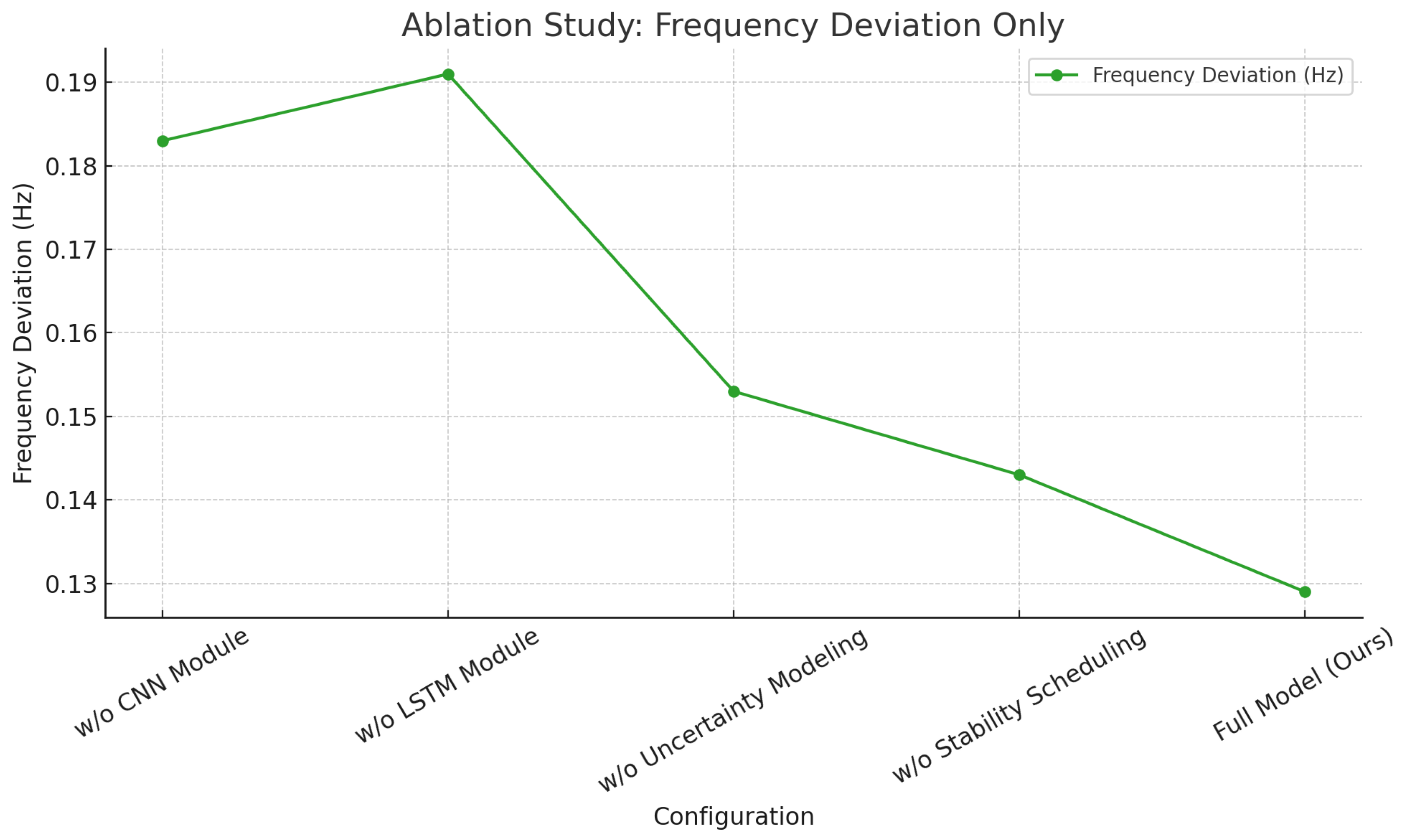
With the increasing uncertainty introduced by the large-scale integration of renewable energy sources, traditional power dispatching methods face significant challenges, including severe frequency fluctuations, substantial forecasting deviations, and the difficulty of balancing economic efficiency with system stability. To address these issues, a deep learning-based dispatching framework is proposed, which integrates spatiotemporal feature extraction with a stability-aware mechanism. A joint forecasting model is constructed using Convolutional Neural Network (CNN) and Long Short-Term Memory (LSTM) to handle multi-source inputs, while a reinforcement learning-based stability-aware scheduler is developed to manage dynamic system responses. In addition, an uncertainty modeling mechanism combining Dropout and Bayesian networks is incorporated to enhance dispatch robustness. Experiments conducted on real-world power grid and renewable generation datasets demonstrate that the proposed forecasting module achieves approximately a 2.1% improvement in accuracy compared with Autoformer and reduces Mean Absolute Error (MAE) and Root Mean Square Error (RMSE) by 18.1% and 14.1%, respectively, compared with traditional LSTM models. The achieved Mean Absolute Percentage Error (MAPE) of 5.82% outperforms all baseline models. In terms of scheduling performance, the proposed method reduces the total operating cost by 5.8% relative to Autoformer, decreases the frequency deviation from 0.158 Hz to 0.129 Hz, and increases the Critical Clearing Time (CCT) to 2.74 s, significantly enhancing dynamic system stability. Ablation studies reveal that removing the uncertainty modeling module increases the frequency deviation to 0.153 Hz and raises operational costs by approximately 6.9%, confirming the critical role of this module in maintaining robustness. Furthermore, under diverse load profiles and meteorological disturbances, the proposed method maintains stable forecasting accuracy and scheduling policy outputs, demonstrating strong generalization capabilities. Overall, the proposed approach achieves a well-balanced performance in terms of forecasting precision, system stability, and economic efficiency in power grids with high renewable energy penetration, indicating substantial potential for practical deployment and further research.

1. Introduction

With the acceleration of global industrialization and the vigorous development of the socio-economic landscape, energy demand has exhibited rapid growth. Renewable energy sources, such as wind and solar power, have gradually emerged as core drivers in the transformation of the global energy structure due to their clean and sustainable characteristics, and have been widely integrated into power systems [1]. By the end of 2020, the installed capacity of renewable energy in China had reached 934,000 MW, representing a year-on-year growth of 17.5% [2]. However, unlike traditional hydropower and thermal power, which are technologically mature and output-stable, renewable energy sources are susceptible to climatic and environmental factors, leading to significant volatility and intermittency. These characteristics substantially increase the uncertainty and fluctuation in power system operations, posing unprecedented challenges to grid stability [3,4]. Under such circumstances, the complexity of power system scheduling has intensified, particularly due to the coupling of dual uncertainties from both the load and renewable generation sides, rendering conventional dispatching strategies increasingly inadequate in addressing these emerging challenges [5]. Traditional dispatching approaches primarily rely on adjustments from conventional generators and centralized control of large-scale power plants. However, the unpredictable and intermittent nature of renewable energy leads to high output variability, making accurate forecasting difficult [6]. Furthermore, although total electricity consumption on the demand side has shown steady growth in recent years, the cumulative duration of peak load events remains short, resulting in disproportionately high costs to meet these rare peaks [7].
The application of deep learning in power systems has led to significant advancements in load forecasting and power output prediction. However, most current forecasting approaches tend to focus on a single type of data, such as relying solely on historical load records or considering only renewable power generation, while lacking comprehensive spatiotemporal modeling capabilities. This omission of spatiotemporal dependencies among variables leads to insufficient predictive accuracy for dynamic system changes, thereby limiting the effectiveness of energy dispatching and operational optimization under stability constraints [8]. Traditional load forecasting models typically concentrate on a single load type—such as electric, cooling, or thermal load—and tend to convert dynamic uncertainty modeling into a static deterministic problem, disregarding periodicity and temporal sequence features [9]. The integration of renewable energy further complicates the relationship between load demand and generation output, exacerbating system uncertainty. The deep integrated learning framework proposed by Ibrahim [10], though capable of constructing multiple deep models, is applicable only to individual or aggregated load forecasting scenarios. Ma et al. [11] noted that existing wind power forecasting techniques often employ decomposition based on a single variable without accounting for the complex interactions between multiple wind-related factors, such as wind speed and wind generation. Tang et al. [12] developed a short-term load forecasting model using temporal convolutional networks (TCNs), which improves forecasting accuracy and generalization but considers only the nonlinear correlation between meteorological features and load demand.
Among widely adopted deep learning models in power forecasting are CNNs and LSTMs. CNNs are effective in capturing local cross-correlations among multiple time series and are capable of extracting high-level features through multiple convolution operations. The local connectivity and global parameter sharing characteristics of CNNs can significantly reduce model parameters and training time [11]. LSTMs, with their ability to learn both long- and short-term dependencies, have shown superior performance in time series modeling and forecasting compared to traditional methods and have proven advantageous for load prediction tasks [9]. In short-term photovoltaic (PV) forecasting, the hybrid CNN-LSTM models described by Ibrahim et al. [13] outperform other conventional models. Wang et al. [9] proposed a dynamic feature extraction method based on an LSTM encoder–decoder (LSTMED) architecture, which surpasses the performance of widely used LSTM and fully connected neural networks (FCNNs), leading to improved load forecasting accuracy. Liu et al. [14] proposed a BiLSTM model with attention mechanisms for short-term PV power forecasting, which effectively extracts key features from multivariate time series and mitigates the impact of weather variability on prediction accuracy. Nonetheless, most existing forecasting methods still overlook spatiotemporal dependencies among input variables, resulting in reduced predictive precision for dynamic system behavior. Moreover, beyond the spatiotemporal forecasting aspect, the core challenge of stability-constrained dispatch lies in incorporating system dynamics into decision making. To this end, a stability-aware scheduling module is introduced to optimize control strategies under frequency and voltage constraints, while an uncertainty modeling mechanism enhances robustness by estimating prediction confidence intervals. These two modules jointly ensure that the scheduling process remains both anticipatory and resilient under fluctuating conditions.
To address these issues, a hybrid forecasting and scheduling framework is proposed, which integrates CNNs and LSTMs to achieve accurate joint forecasting of load demand and renewable generation in power systems. A CNN-LSTM hybrid network is first introduced to extract short-term local features via CNNs and capture long-term temporal dynamics via LSTMs, enabling multitask forecasting of both load and renewable outputs. This structure balances localized feature extraction and temporal modeling, capturing key fluctuation patterns in load and generation, thereby guiding stability-enhancing dispatch strategies. Furthermore, a stability-aware scheduling module is designed to minimize operational costs while incorporating frequency deviation and voltage fluctuation constraints. The resulting optimization problem is solved using either heuristic search or reinforcement learning techniques. Finally, uncertainty modeling and robustness optimization are incorporated through Monte Carlo Dropout and Bayesian neural networks to estimate predictive confidence intervals, enabling the dispatch strategy to incorporate robustness under forecast volatility. This ensures high forecasting performance and scheduling efficiency in real-world deployment scenarios. The main contributions of this study are summarized as follows:
1.
A CNN-Transformer hybrid model is constructed to enable accurate forecasting of multivariate time series in power systems.
2.
A stability-aware scheduling optimization module is introduced to ensure frequency and voltage stability under high renewable penetration.
3.
The effectiveness and generalization capability of the proposed framework are validated on multiple real-world power system datasets, showing significant improvements over state-of-the-art baseline models.

2. Related Work

2.1. Development of Power Load and New Energy Prediction Methods

Time series forecasting represents one of the most critical tasks in both scientific and industrial domains, particularly in the field of energy consumption [15]. By leveraging historical data to predict future values, power systems can achieve timely scheduling, resource allocation, and supply–demand balancing [16]. Common statistical approaches for time series forecasting include autoregressive integrated moving average (ARIMA) and support vector regression (SVR), which have been widely applied to energy demand forecasting. However, these methods exhibit notable limitations when applied to power system forecasting tasks [16].
The ARIMA method integrates autoregressive (AR), integrated (I), and moving average (MA) processes and is widely used for load forecasting. For a time series x with n instances, the ARIMA model is defined as:
x k = i = 1 p A i x k i + j = 1 q B j v k j + v k
where v k is an m-dimensional vector of uncorrelated random noise with zero mean and covariance matrix R, p denotes the order of autoregression, and q represents the order of lagged forecast errors. Fara et al. [17] demonstrated that ARIMA outperformed ANN in short-term solar forecasting. Elsaraiti et al. [18] applied ARIMA to household electricity consumption forecasting with high accuracy. Nepal et al. [19] proposed a hybrid model combining clustering and ARIMA to forecast campus electricity load, achieving high peak-time accuracy. The SVR model is a popular machine learning method that maps input data into a high-dimensional feature space via kernel functions, where a linear regression function is constructed [20]:
f ( x ) = ω · φ ( x ) + b
where x is the input data, f ( x ) is the regression function, and  φ ( x ) denotes the transformation into the feature space. Despite its effectiveness, SVR performs poorly on highly volatile and periodic data. Meng et al. [21] showed that SVR outperformed linear and Grey models in energy usage forecasting. Yan et al. [22] developed an SVR-based model accounting for the coupling of electrical, cooling, and heating loads. Rao et al. [23] introduced an SVR-based CDSES model to forecast primary energy demand over the next decade. In recent years, deep learning models such as LSTM, GRU, and Transformer have demonstrated superior modeling capability and adaptability in power forecasting. LSTM has shown improved performance in volatile data environments due to its ability to capture long-term dependencies through gated mechanisms [24,25]. The LSTM cell is defined as follows [26]:
f t = σ W t · [ h t 1 , x t ] + b t
i t = σ W i · [ h t 1 , x t ] + b i
o t = σ W o · [ h t 1 , x t ] + b o
where f t , i t , and  o t represent the forget, input, and output gates, respectively, and  σ denotes the sigmoid function. Jailani et al. [27] found that LSTM achieved high accuracy in solar radiation and photovoltaic forecasting. Jin et al. [28] proposed a PLSTM model enhanced by singular spectrum analysis (SSA), outperforming state-of-the-art models in accuracy and efficiency. Wang et al. [29] demonstrated that LSTM surpassed ARMA, ARFIMA, and BP methods in long-term energy consumption prediction. GRU operates similarly to LSTM but with fewer gates and no separate cell state, relying instead on hidden state transitions to retain long-term memory [24]. Iruela et al. [30] enhanced GRU training using GPU-based parallelized PSO, improving both training speed and prediction accuracy. In [31], a GPU-based NGSA-II model was used for public building energy forecasting, achieving faster computation and improved results. Iruela et al. [32] utilized advanced ANN and GPU architecture to improve energy consumption forecasting. Transformer models are encoder–decoder architectures built on self-attention mechanisms [33]. These models allow efficient parallel computation and excel at handling long sequences and large-scale data, effectively mitigating gradient-related issues in RNNs and improving training speed and stability [34]. Galindo et al. [35] incorporated Transformer in renewable energy forecasting systems, achieving strong performance across environments. Wang et al. [36] developed the MultiDeT Transformer-based multitask model for joint multi-load forecasting with high generalization. L et al. [37] proposed a Transformer-based load forecasting framework that effectively captured time-series context and outperformed Seq2Seq models.
Although the above methods have shown promise, power systems are characterized by complex spatiotemporal features, including spatial load distribution, renewable output fluctuations, and dynamic grid structures. Most existing models overlook these coupled dimensions, leading to suboptimal coordination in complex environments [38].

2.2. The Application of Deep Learning in Power System Dispatch Optimization

With the rapid development of smart grids and renewable energy, energy dispatch has become increasingly complex. Reinforcement learning (RL) and deep optimization methods have emerged as effective tools. RL learns optimal policies through interactions with the environment to maximize long-term rewards, while deep reinforcement learning (DRL) enhances expressive power via neural networks. Xu et al. [39] introduced a multi-agent deterministic policy gradient (MADDPG) algorithm for integrated energy systems (IES), achieving enhanced optimization and stability. Yang et al. [40] proposed a model-free DRL-based dynamic dispatch policy with improved cost-efficiency and adaptability. Ebrie et al. [41] applied RL for power dispatch optimization in both renewable-integrated and conventional systems. Jiang et al. [42] built a deep Q-network (DQN)-based short-term optimal dispatch model for hydro–wind–solar systems, improving decision making and efficiency. Despite promising results, current DRL approaches primarily focus on single-source data, overlooking spatiotemporal correlations. The rising share of renewables further challenges real-time dispatch, requiring synchronization with ultra-short-term forecasting—a gap yet to be addressed [43]. Moreover, existing methods emphasize economic objectives while neglecting the joint optimization of stability and cost. Although DRL improves renewable utilization and economic efficiency over traditional methods, further refinement is needed to ensure stable and economical dispatch in dynamic environments [44].

2.3. Load—New Energy Coordinated Scheduling and System Stability

With the widespread integration of renewable energy, distributed generation, and storage systems, power grid operation has become more intricate. These multi-source inputs introduce significant variability and uncertainty, enhancing flexibility and sustainability but also posing challenges to system stability. Particularly, renewable sources such as wind and solar influence load balance and power dispatch, thus affecting grid stability [45]. Transient stability refers to the short-term response of the grid to disturbances [46]. High renewable penetration and source variability can lead to transient instability through abrupt load or voltage fluctuations. Zhou et al. [47] developed a multi-channel CNN model for accurate transient stability prediction. Fan et al. [48] analyzed system frequency stability under major disturbances using Lyapunov methods. As conventional generator inertia and frequency regulation decline with increasing renewable penetration, energy storage systems become critical for frequency control due to their rapid response and efficiency [49]. Li et al. [50] proposed a coordinated converter-based frequency scheduling model to ensure frequency safety. Further, the significance of frequency regulation was explored through FOR, PFR, and IR perspectives [51]. Hence, stability is not only foundational to grid operation but also a prerequisite for intelligent and efficient dispatch. Ensuring transient stability, frequency regulation, and fast system response is essential for addressing challenges from multi-source integration.

3. Materials and Method

3.1. Data Collection

The dataset utilized in this study encompasses multiple dimensions, including load power, wind and photovoltaic generation, meteorological conditions, grid operational states, and scheduling records. The data spans from 2018 to 2022, with a uniform sampling interval of 15 min to ensure continuity and consistency for time-series modeling and scheduling response simulation. Load data were obtained from an actual power grid monitoring system in a region of North China, covering various types of consumers such as residential areas, industrial zones, and commercial centers. These data exhibit clear daily and weekly periodic patterns, with pronounced peaks and troughs during summer and winter, which facilitates the evaluation of model performance under complex and volatile conditions, as shown in Table 1. Wind and photovoltaic generation data were collected from the National Energy Administration’s renewable energy monitoring platform, as well as from a partner wind farm and solar power station via SCADA systems. The wind dataset includes wind speed, direction, blade pitch angle, and real-time output of turbines, while the photovoltaic dataset comprises solar irradiance, module temperature, and inverter output power. To enhance the model’s ability to capture weather influences, hourly station-level meteorological observations from the China Meteorological Administration were incorporated, covering variables such as temperature, humidity, precipitation, pressure, wind speed, and wind direction. In certain regions, supplementary measurements were collected through ground-based automatic weather stations (AWS), and transmitted via LoRa communication modules to a cloud platform to ensure real-time updates and broad spatial coverage. Grid operational data include system frequency, voltage, phase angle, and regulation margin, collected through remote terminal units (RTUs) deployed in this project and transmitted using the IEC 60870-5-104 protocol. All signals were preprocessed using noise filtering and time synchronization techniques. Additionally, scheduling instructions and execution records were obtained from the grid control platform, involving generator start/stop commands, energy storage charge/discharge instructions, and demand-side response logs, which were used to train and evaluate the stability-aware scheduling strategy. During data integration, all records were aligned using a unified timestamp, and missing values were handled through a hybrid method combining sliding window mean interpolation and k-nearest neighbor imputation. Outliers were removed using the interquartile range (IQR) method. Ultimately, a dataset containing over one million samples was constructed, characterized by strong temporal dependency, heterogeneity, and uncertainty, thereby providing a robust foundation for model generalization across diverse data sources.

3.2. Data Preprocessing and Augmentation

In the context of deep learning modeling, the quality of input data directly determines both the predictive performance and generalization capability of the model. Due to common issues in power system and meteorological monitoring data—such as measurement noise, missing values, and inconsistent scales—appropriate preprocessing and augmentation prior to modeling are essential to ensure convergence stability and predictive accuracy. To eliminate anomalous values (e.g., extreme readings caused by sensor faults) that may adversely affect model training, a threshold-based statistical method was applied. For a given time series feature x t t = 1 T with mean μ and standard deviation σ , any data point satisfying the following condition was identified as an outlier and removed:
| x t μ | > k σ ,
where the hyperparameter k is typically set to 2 or 3 based on empirical sensitivity. Removed values were subsequently processed as missing entries. For natural missing values in the observation data, a hybrid method combining moving average and linear interpolation was adopted. Specifically, for missing locations t k M [ 1 , T ] , a window length w was defined, and the estimated value of the missing point x t k was computed as:
x ^ t k = 1 | W t k | i W t k x i ,
where W t k = { t k w , , t k 1 , t k + 1 , , t k + w } [ 1 , T ] denotes the set of valid observations surrounding the missing index. For continuous missing segments or boundary cases, linear interpolation was applied:
x ^ t k = x t a + t k t a t b t a ( x t b x t a ) ,
where t a < t k < t b , and  x t a , x t b represent the closest valid observations on either side of the gap. To eliminate the influence of differing feature scales during model training, all input variables were normalized using min-max scaling, mapping each x t into the interval [ 0 , 1 ] as follows:
x t norm = x t min ( x ) max ( x ) min ( x ) ,
where min ( x ) and max ( x ) denote the minimum and maximum values of the feature in the training set, respectively. To enhance robustness under anomalous operating conditions and increase sample diversity, data augmentation was further conducted. The objective of augmentation was to generate representative pseudo-samples by perturbing the original inputs, thereby improving model generalization to low-probability extreme scenarios. Specifically, given an original input sequence x = { x 1 , x 2 , , x T } , Gaussian perturbations were introduced to create augmented samples:
x ˜ t = x t + ϵ t , ϵ t N ( 0 , σ 2 )
where the standard deviation σ was empirically selected according to the characteristics of each feature, ensuring that the perturbed data remained statistically consistent with the original distribution. Following the above procedures, a structured multi-input sequence was constructed, comprising recent power load values, wind and photovoltaic outputs, and meteorological variables (e.g., wind speed, solar irradiance, temperature, and humidity), thereby providing a high-quality input foundation for subsequent predictive modeling.

3.3. Proposed Method

The overall framework of the proposed model begins at the data input stage. The preprocessed multi-dimensional time-series data are first simultaneously fed into the spatiotemporal fusion forecasting module. Within this module, local features are extracted using a CNN, while sequential dependencies are captured by a LSTM network. The outputs include load demand and renewable energy forecasts. These forecast results, together with the current system state, are subsequently input into the stability-aware scheduling module, which generates dispatch strategies that satisfy both frequency and voltage constraints. In parallel, the uncertainty modeling module provides confidence intervals for predictions, serving as robustness constraints in scheduling optimization. Together, the three components form an integrated and efficient closed-loop control framework.

3.3.1. Spatiotemporal Forecasting Module (CNN-Transformer Hybrid Network)

The spatiotemporal forecasting module is designed to perform high-precision modeling of multi-source time-series data in power systems, enabling the joint forecasting of load demand and renewable energy generation. As shown in Figure 1, the module consists of a CNN encoder and stacked Transformer layers, facilitating both local spatial feature extraction and long-range temporal dependency modeling. To capture spatial heterogeneity and inter-regional dependencies within the power grid, spatial modeling is incorporated at both the data input and model design stages. First, multivariate sequences from each region (e.g., A, B, and C) are stacked as separate channels to form a 3D input tensor of shape (R × T × F), where R denotes the number of regions, T the time window length, and F the feature dimension per region. This channel-wise spatial structure enables CNN filters to extract localized variations across regions. In the scheduling module, a spatial-aware state embedding is constructed for each node, incorporating geographical coordinates, controllable power capacity, and local load fluctuation statistics. These node embeddings are embedded into the reinforcement learning state space, allowing the scheduling policy to adapt to topological and regional dynamics effectively. This explicit spatial integration enhances the model’s responsiveness to geographically distributed grid conditions.
The input is a three-channel tensor with dimensions 3 × 300 × 300 , representing concatenated time-window sequences of load, wind power, and meteorological variables. Two 1D convolutional layers are applied to extract local features. Unlike conventional time series image encoding techniques such as Gramian Angular Fields (GAFs) or Recurrence Plots (RPs), this study constructs pseudo-image tensors directly through sliding-window segmentation. Specifically, for each time window, sequences of load demand, renewable generation, and meteorological observations are normalized and stacked as three channels to form a tensor of shape 3 × 300 × 300. The first dimension indexes modalities, while the second and third dimensions correspond to time steps and feature dimensions, respectively. This format allows the CNN encoder to capture localized spatial–temporal patterns across modalities without explicit image transformation. The first layer uses a kernel size of 5, increasing the number of channels from 3 to 16, producing feature maps of size 150 × 150 . Group normalization and ReLU activation are applied, followed by a second convolutional layer that extracts higher-order spatiotemporal features with 32 channels and output size 75 × 75 . This stage captures short-term fluctuations, trend shifts, and spatially homogeneous patterns in the time series, thereby generating discriminative low-level representations for the prediction tasks. The final output is flattened into a 1D vector of size 1 , 800 , 000 and projected linearly into a 7 × 512 time-embedded representation as input to the Transformer layers.
The Transformer component consists of two standard encoder blocks, each containing a multi-head self-attention mechanism and a feedforward network. The model dimension is d model = 512 , divided into 8 heads, each with dimensions d q = d k = d v = 64 . For each head, query, key, and value matrices Q i , K i , and  V i are computed via linear projections. Attention weights are calculated as A i = Softmax ( Q i K i T / d k ) , and the weighted outputs are Z i = A i V i . The outputs from all heads are concatenated and projected linearly to produce the block output Z. This attention mechanism allows the model to capture dependencies across arbitrary time steps, making it particularly suitable for modeling load peaks, weather-induced fluctuations, and other temporal patterns in power systems.
Following the Transformer, the feedforward network includes two fully connected layers separated by a ReLU activation function, with a hidden size of 1024 and output dimension d model . This enhances nonlinear transformation capacity and enables the learning of complex forecasting patterns. The output of the stacked blocks serves as the final predictive encoding vector, which is used to drive downstream multi-task regression modules.
This module offers several advantages. The CNN captures high-frequency local variations and handles sudden changes in load or renewable generation. The Transformer enhances mid- to long-term dependency modeling, allowing the network to better learn periodic and trend information. Structurally, the module fuses local and global spatiotemporal information, generating robust representations that enable more accurate and reliable dispatch optimization. Furthermore, its parameters can be adaptively adjusted based on regional or seasonal characteristics, improving generalization across diverse power system contexts. Theoretically, by minimizing the forecasting loss L forecast = α · MSE load + β · MSE renewable , the module balances predictive accuracy with inter-task correlation, achieving effective co-modeling of load and renewable forecasts.

3.3.2. Stability-Aware Scheduling Module

The stability-aware scheduling module serves as the core decision-making component, aiming to minimize operational costs while maintaining system stability under high renewable penetration. Frequency deviations and voltage fluctuations introduced by variable generation are explicitly accounted for in the scheduling process. This module is implemented using an Actor–Critic reinforcement learning architecture, with a state representation that integrates system conditions, node resources, and task dynamics. Expert demonstrations and experience replay are incorporated to accelerate training and improve policy robustness.
As shown in Figure 2, the Actor receives the system state s t k at each timestep, including current load distribution, controllable node state s t node , k , and renewable output state s t ms , k . These are encoded using linear layers to produce e t ms , k R 128 and e t node , k R 128 , with linear transformations W R 128 × d in and bias b R 128 for d in = 64 . The node state is further processed by a single-layer gated recurrent unit (GRU) with hidden dimension 256 to model sequential dependencies. The concatenated encodings are mapped via W f R 256 × ( 128 + 256 ) and passed through a softmax layer to yield the action probability distribution:
π ( a t k | s t k ) = Softmax ( W f [ e t ms , k , h t ] + b f )
Actions a t k are then sampled from the space a 1 , a 2 , , a N as dispatch decisions.
The Critic evaluates the soft value of selected actions by processing the concatenated state–action pair ( s t k , a t k ) through two linear layers with ReLU activations and output size 512. The Soft Q-value is computed as:
Q π ( s t k , a t k ) = E l = 0 γ l r t + l k α · log π ( a t + l k | s t + l k )
where γ denotes the discount factor and α is the entropy regularization coefficient that encourages exploration. The training follows the Soft Actor–Critic (SAC) algorithm with mini-batch updates from a replay buffer. Behavior cloning with expert policy π b is applied during pretraining to improve initial policy performance and convergence.
When integrated with the spatiotemporal forecasting module, this scheduling component receives predicted future load L ^ t : t + T and renewable outputs R ^ t t + T as part of the state input, enabling anticipatory decision making. The theoretical basis lies in extending the observable space of a Markov decision process (MDP) with prior forecast variables. Given true state s t and forecast output o t , the augmented state becomes s t = [ s t , o t ] , and the objective is defined as:
π * = arg max π E s t D Q π ( s t , a t )
To balance economic efficiency with system stability, the reinforcement learning agent is trained using the following multi-objective reward function:
r k = λ 1 · C k λ 2 · | Δ f k |     λ 3 · | Δ V k |
where C k denotes the operational cost at step k, Δ f k is the system’s frequency deviation, and  Δ V k is the voltage fluctuation magnitude. The coefficients λ 1 , λ 2 , and  λ 3 are hyperparameters that control the trade-off among cost, frequency, and voltage stability. This reward design explicitly penalizes unstable states while promoting cost-effective scheduling, and is integrated into the Soft Actor–Critic (SAC) training process alongside experience replay and behavior cloning. Experimental results demonstrate that incorporating stability terms significantly improves frequency deviation and critical clearing time, validating the effectiveness of the proposed formulation. This design forms a closed loop of perception, prediction, and decision making, significantly improving robustness under uncertainty, especially during frequency violations, severe weather, or rapid renewable fluctuations.

3.3.3. Uncertainty Modeling and Robust Optimization Module

The uncertainty modeling and robust optimization module addresses potential distributional shifts and extreme perturbations in forecasting, enhancing the robustness of the scheduling process in practical deployments. This module leverages Bayesian deep learning and predictive confidence estimation mechanisms based on CNN-Transformer outputs. Two approaches are adopted: a non-parametric method using Monte Carlo Dropout and a Bayesian LSTM with posterior approximation. The resulting confidence intervals are embedded into the scheduling objective to handle volatile conditions. To capture uncertainty across both spatial and temporal dimensions, the framework integrates Monte Carlo Dropout and Bayesian LSTM. Specifically, Monte Carlo Dropout is employed during inference on the CNN-based encoder to estimate predictive variance by performing multiple stochastic forward passes. This captures uncertainty arising from spatial representation variability. On the other hand, Bayesian LSTM models the uncertainty in temporal dependencies by treating the LSTM weights as distributions and updating them via variational inference. The combination of these two approaches enables a comprehensive characterization of prediction uncertainty, which is crucial for robust scheduling under dynamic grid conditions. Empirical results confirm that the dual uncertainty modeling strategy enhances the system’s responsiveness to rare fluctuations and improves scheduling robustness.
Dropout layers are appended after the LSTM output, remaining active during inference. Multiple forward passes ( T = 50 ) with dropout probability p = 0.2 are performed to obtain predictive distributions. The predictive mean y ^ t and uncertainty bound δ t are computed as:
y ^ t = 1 T i = 1 T f ( i ) ( x t ) , δ t 2 = 1 T i = 1 T ( f ( i ) ( x t ) y ^ t ) 2
where f ( i ) ( x t ) denotes the i-th forward result. The confidence interval y ^ t δ t , y ^ t + δ t is then used as a constraint for robust scheduling.
To further enhance probabilistic consistency, a Bayesian LSTM is constructed by replacing LSTM weights with distributions. Variational inference is employed to approximate the posterior. The network has two LSTM layers (hidden size 128) followed by ReLU activations and linear mappings to output the predictive mean and variance ( μ t , σ t 2 ) . The loss is the negative log-likelihood:
L Bayes = t ( y t μ t ) 2 2 σ t 2 + 1 2 log σ t 2
The KL-divergence regularization is defined as:
L KL = KL ( q ( W ) | p ( W ) ) = i q ( w i ) log q ( w i ) p ( w i )
yielding the total loss:
L total = L Bayes + β · L KL
where β adjusts the balance between prior regularization and data fitting.
This module is integrated with the stability-aware scheduler by feeding the uncertainty bound δ t as a constraint. For instance, the generation dispatch is bounded by:
P gen , t L ^ t + γ · δ t
where γ = 1.64 corresponds to a 90% confidence level. This ensures sufficient reserves under forecast exceedance, preventing frequency drops or load shedding. The same mechanism can be extended to storage sizing and reserve margin allocation. The algorithm is summarized in Algorithm 1. To enhance the agent’s awareness of future system dynamics, the outputs from the forecasting module—namely the predicted future load and renewable generation y ^ t and the corresponding uncertainty δ t —are incorporated into the reinforcement learning state space. Specifically, the agent’s state at each decision step is augmented as:
s k = [ s k , y ^ t , δ t ] ,
where s k includes current system observations such as node loads, voltage levels, frequency values, and energy storage status. The term y ^ t provides forward-looking estimations, while δ t conveys the forecast confidence range (e.g., standard deviation or confidence interval width). This augmented state s k is input into the Actor–Critic framework, enabling the policy to make risk-aware and anticipatory decisions. Experimental results demonstrate that this integration substantially improves both frequency regulation and robustness under high-uncertainty disturbances.
Algorithm 1: Uncertainty Modeling and Robust Scheduling Pseudocode
Information 16 00662 i001

4. Results and Discussion

4.1. Experimental Setup

4.1.1. Data Split

The experiments were conducted based on multiple real-world power system datasets, encompassing wind and photovoltaic power output, meteorological observations, and load dispatch records collected from various regions between 2018 and 2022. These datasets exhibit strong representativeness and diverse spatiotemporal coverage. To ensure sufficient training and objective evaluation, all data were uniformly divided into training and testing sets in a ratio of 80% to 20%, respectively. The training set was used for model parameter learning, while the testing set served to evaluate the model’s generalization performance on previously unseen data. To further assess the adaptability and robustness of the proposed model under varying operational conditions, the testing set included several representative scenarios, such as clear versus overcast days, as well as peak load conditions in winter and trough load conditions in summer. By constructing a diverse distribution of samples, various extreme operational states were simulated to comprehensively evaluate forecasting and scheduling performance under high uncertainty. This evaluation strategy, grounded in real system data and multi-scenario partitioning, enhances the breadth and depth of performance analysis, thereby ensuring the transferability and reliability of experimental results in practical engineering applications.

4.1.2. Evaluation Metrics

To comprehensively evaluate the proposed method in terms of forecasting accuracy, economic efficiency, and operational stability, a multi-dimensional evaluation metric system was designed. Specifically, for forecasting accuracy, three widely adopted regression metrics were employed: MAE, RMSE, and mean absolute percentage error (MAPE). In the context of scheduling optimization, the total operation cost was introduced to assess the economic performance of the scheduling strategy. With regard to system stability, two critical indicators were considered: frequency deviation and critical clearing time (CCT). The mathematical definitions of these metrics are presented as follows:
MAE = 1 N i = 1 N y ^ i y i
RMSE = 1 N i = 1 N y ^ i y i 2
MAPE = 100 % N i = 1 N y ^ i y i y i
Cos t total = t = 1 T g = 1 G C g ( P g , t )
Δ f = max t f t f nom
CCT : obtained via time - domain transient stability simulation
Here, MAE quantifies the average absolute deviation between predicted and actual values, serving as a fundamental measure of overall error magnitude. RMSE emphasizes large prediction errors due to the squared term, making it suitable for evaluating model robustness under abrupt or extreme fluctuations. MAPE expresses relative error as a percentage, allowing consistent comparisons across heterogeneous variables. Regarding economic evaluation, the total operation cost Cos t total aggregates the operational expenditures of all generation units over the entire scheduling horizon, directly reflecting the cost-optimization capability of the model. In terms of stability assessment, the frequency deviation Δ f captures the maximum deviation of system frequency from its nominal value, serving as a key indicator of dynamic equilibrium. The critical clearing time (CCT) represents the maximum tolerable fault duration before system instability occurs, with larger values indicating greater transient stability margins. The integration of these diverse metrics ensures a holistic assessment of the proposed method under complex, real-world power system conditions, thereby validating its practical feasibility and engineering applicability.

4.1.3. Baseline

To validate the effectiveness of the proposed method in forecasting power load and renewable energy output, five representative models were selected as comparative baselines, including the LSTM [52], the gated recurrent unit network (GRU) [53], support vector regression (SVR) [54], a single CNN model [55], and Autoformer [56], a recent Transformer-based architecture with strong performance in time series forecasting. These models have been widely applied in sequential prediction tasks and are recognized for their distinctive advantages, enabling a comprehensive evaluation of the proposed method from multiple perspectives. As classical recurrent neural architectures, LSTM and GRU possess strong capabilities in capturing temporal dependencies and exhibit stable performance in modeling mid- to long-term trends, making them among the most frequently used deep learning approaches for load and output prediction. SVR, a traditional statistical learning method, excels in nonlinear regression under small-sample conditions and offers robust theoretical interpretability and generalization ability. The standalone CNN model is capable of rapidly extracting local patterns in time series through convolutional kernels, achieving a favorable trade-off between computational efficiency and expressive power. Autoformer, a recent advancement in Transformer-based forecasting, introduces adaptive trend modeling and series decomposition mechanisms, yielding superior accuracy and robustness, particularly in long-term forecasting scenarios. Through comparison with these structurally diverse and functionally distinct models, the performance gains and generalizability of the proposed approach across different scenarios and evaluation dimensions can be thoroughly substantiated.

4.1.4. Hardware and Software Platform

All model training and experimental evaluations were conducted on a high-performance computing platform equipped with dual NVIDIA RTX 4090 GPUs (Manufacturer: NVIDIA Corporation, Santa Clara, CA, USA), each with 24 GB of memory, and an AMD Ryzen 9 5950X processor (Manufacturer: Santa Clara, CA, USA), supported by 128 GB of DDR4 RAM. The operating system environment was based on Ubuntu 22.04 LTS. Python 3.10 served as the core programming language, and the model implementations were built using PyTorch 2.1.0 with CUDA 11.8 acceleration. Additional dependencies included NumPy for numerical operations, SciPy for statistical analysis, Pandas 2.3 for data handling, and Matplotlib 3.10 and Seaborn 0.13 for visualization. All neural network models, including LSTM, GRU, CNN, Autoformer, and the proposed CNN-Transformer hybrid architecture, were trained using the Adam optimizer with a learning rate of 1 × 10 3 and a batch size of 64. Gradient clipping was applied with a maximum norm of 5.0 to stabilize training. Early stopping with a patience threshold of 15 epochs was employed to avoid overfitting. For the reinforcement learning component, the Soft Actor–Critic (SAC) algorithm was implemented using the RLlib framework from Ray 2.5.0. Hyperparameters such as the entropy coefficient α and discount factor γ were selected via grid search on the validation set. All experiments were reproducible, with fixed random seeds across modules, and were executed in isolated virtual environments to ensure consistency in dependency versions. The hardware configuration and software stack collectively ensured efficient training convergence, scalability of experimentation, and compatibility with large-scale power system datasets.

4.2. Forecasting Performance Comparison

This experiment was designed to evaluate the effectiveness of the proposed CNN-Transformer hybrid forecasting model in the joint prediction of renewable energy output and power load, and to compare its performance with that of mainstream time-series modeling approaches. By assessing model performance across three error metrics—MAE, RMSE, and MAPE—it becomes possible to comprehensively evaluate each model’s predictive accuracy, stability, and error control capabilities.
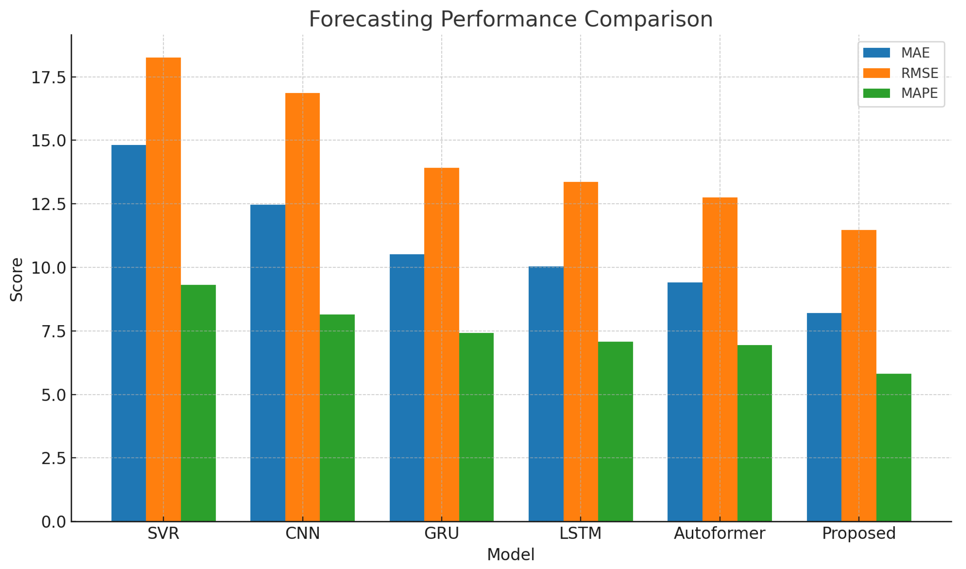
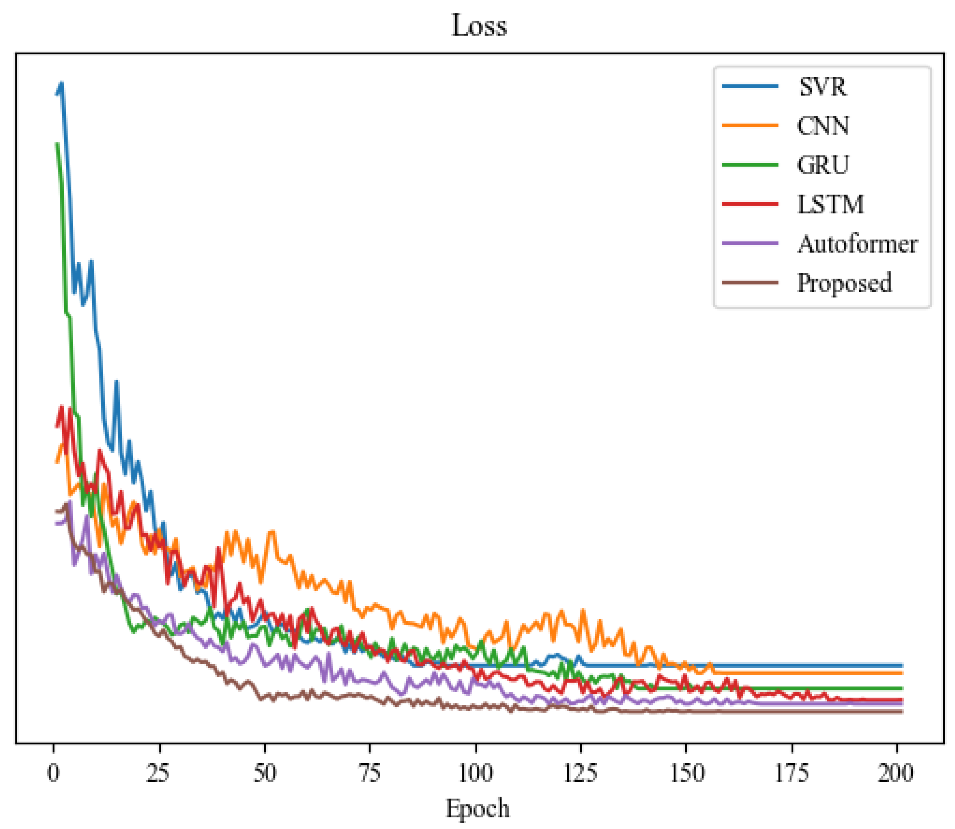
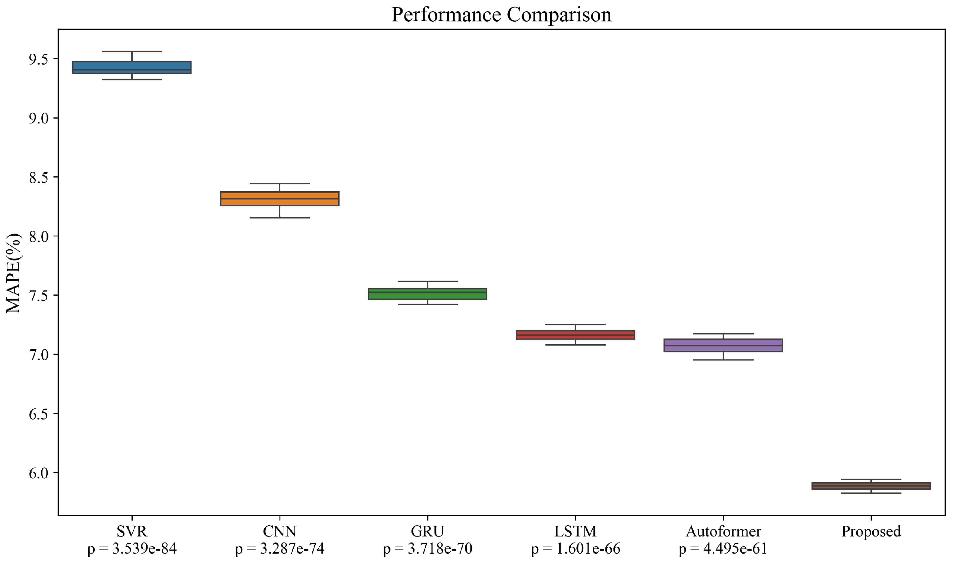
As shown in Table 2 and Figure 3, Figure 4, Figure 5 and Figure 6, support vector regression (SVR) exhibited the worst performance with a MAPE of 9.32%, owing to its lack of temporal modeling capabilities. Although CNN is capable of extracting local spatial features, it fails to model temporal dependencies effectively, resulting in considerable prediction error. GRU and LSTM, as typical recurrent neural networks, performed better in modeling short-term temporal dependencies, thus achieving superior error metrics compared to SVR and CNN. Autoformer, a recent Transformer-based architecture with self-attention, further reduced prediction errors due to its strength in modeling long-range temporal structures. The proposed CNN-Transformer model outperformed all baselines across the three metrics, demonstrating strong generalization ability and high predictive accuracy, thereby validating the effectiveness of integrating hierarchical feature extraction with sequence modeling. From a structural and mathematical perspective, SVR is essentially a static regression model and lacks the capacity to capture dynamic evolution in the data, which explains its poor performance under highly volatile load and renewable output conditions. CNN has strong local pattern extraction capabilities, enabling it to detect short-term trends and fluctuations, but lacks a global temporal modeling mechanism, making it less responsive to periodic load patterns. GRU and LSTM mitigate the gradient vanishing issues in traditional RNNs through gating mechanisms, allowing them to model temporal trends and cycles more effectively; however, their relatively shallow architecture limits their performance under simultaneously volatile and periodic input conditions. Autoformer leverages time-aware self-attention to model long-range dependencies, yet exhibits some limitations in detecting short-term disruptions. In contrast, the proposed model leverages CNN for short-term disturbance extraction and LSTM for modeling temporal sequences, resulting in dual modeling capabilities for both micro-level volatility and macro-level trends. This structural alignment with task-specific demands ultimately leads to superior performance in both accuracy and robustness.

4.3. Economic Cost and Stability Performance Comparison

This experiment aimed to evaluate the integrated control capabilities of different forecasting models within the context of dispatch optimization, with a particular focus on economic performance and dynamic system stability. By comparing total operational costs, frequency deviations, and critical clearing times (CCT), this analysis offers a comprehensive assessment of how prediction accuracy influences both economic and stability aspects of power systems.
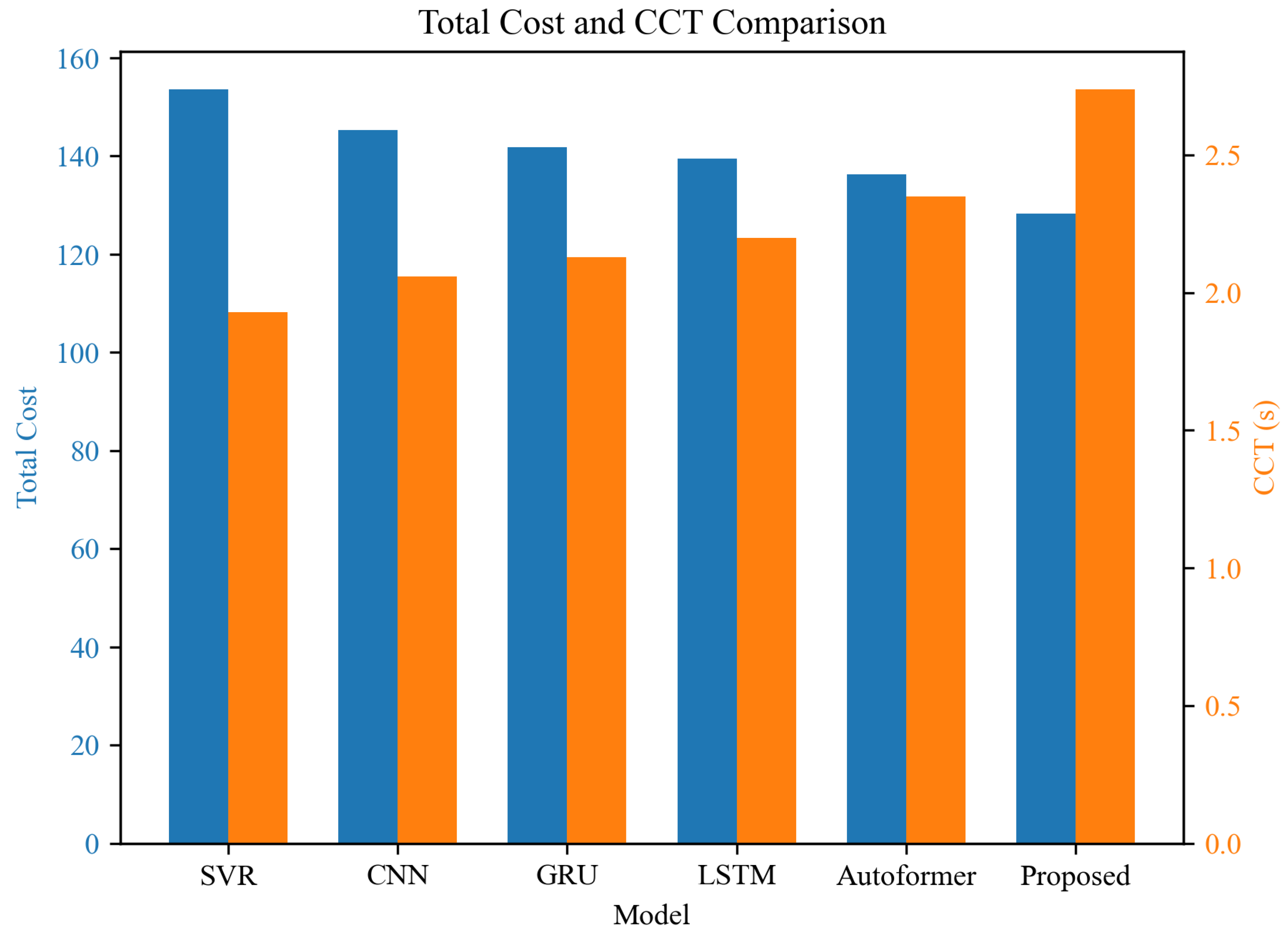
As shown in Figure 7 and Table 3, SVR exhibited the highest total cost of 153.6 due to its large prediction errors, leading to conservative and economically inefficient dispatch decisions. Its frequency deviation reached 0.238 Hz, and the CCT was limited to 1.93 s, indicating the weakest system stability. While CNN improved local trend detection, the lack of long-term modeling limited its dispatch performance. GRU and LSTM provided better results in both cost and stability. Autoformer further enhanced the system’s ability to manage frequency fluctuations, increasing the CCT to 2.35 s. The proposed model achieved optimal performance in all three metrics, reducing the total cost to 128.3, controlling frequency deviation to 0.129 Hz, and extending CCT to 2.74 s. These improvements clearly demonstrate the direct impact of forecasting accuracy on dispatch optimization outcomes. From a mathematical modeling standpoint, SVR relies on static kernel-based regression and lacks responsiveness to dynamic system changes, resulting in significant dispatch errors and the need for excessive reserve capacity. CNN captures local patterns in short time windows and mitigates lag in dispatch decisions, but its convolutional structure does not offer global memory, limiting its ability to address frequency shifts induced by external disturbances. GRU and LSTM improve memory of historical patterns through gating units, enabling more informed dispatch decisions. Autoformer relies on self-attention mechanisms to construct long-range dependencies and global state awareness, thus enhancing overall stability. The proposed model integrates CNN for local disturbance feature extraction and LSTM for long-term dynamic trend modeling, and jointly applies reinforcement learning to form a stability-aware closed-loop scheduling strategy. This results in fast response to disturbances, forward-looking decision making, and a substantial reduction in operational costs and frequency deviations, achieving significant gains in both safety and economic performance.

4.4. Ablation Study of Key Modules

This experiment was designed to evaluate the independent and collaborative contributions of key model components by systematically removing each module. The effects of excluding the CNN module, LSTM module, uncertainty modeling module, and stability-aware scheduling module were analyzed in terms of forecasting accuracy, operational cost, and frequency deviation.
As shown in Table 4, removing the CNN module increased MAE to 10.74, indicating a reduction in the model’s ability to respond to short-term disturbances. Eliminating the LSTM module further degraded MAE to 11.26, raised operational costs to 147.2, and caused larger frequency deviations. Omitting the uncertainty modeling mechanism led to increased costs 137.1 and higher frequency deviation (0.153 Hz), although prediction accuracy remained better than conventional models. Without the stability-aware scheduling module, frequency control was weakened despite acceptable forecasting performance. Only the full model achieved optimal results across all metrics, highlighting the synergistic effect of the integrated modules. From a mathematical perspective, CNN enables the model to detect short-term, high-frequency disturbances via localized receptive fields. Its removal causes the input sequence to lose sensitivity to sudden fluctuations, reducing the scheduler’s responsiveness. LSTM introduces gated mechanisms to retain critical historical states, essential for capturing cyclical trends and renewable output patterns. Its absence leads to a short-sighted model with reduced anticipatory capability. Uncertainty modeling, whether through Bayesian inference or Monte Carlo dropout, provides confidence bounds that constrain scheduling decisions under volatile conditions. Without it, the system becomes risk-prone and may oscillate between over-conservative and over-aggressive strategies. The stability-aware module applies reinforcement learning to minimize penalties for frequency and voltage deviations, forming the core feedback loop between forecasting and decision making. Collectively, these modules are not only independently valuable but also structurally complementary, forming a predictive, controllable, and uncertainty-aware intelligent dispatch system.

4.5. Robustness Evaluation on Public SmartMeter Dataset

The objective of this experiment is to evaluate the generalization ability and robustness of the proposed model on the publicly available SmartMeter dataset [57]. Compared with proprietary datasets, the SmartMeter dataset contains a large volume of household electricity consumption records across diverse users and time periods, exhibiting more complex and volatile load patterns. Therefore, it serves as a more objective benchmark for assessing the stability of model predictions under realistic and dynamic scenarios. Across all models, performance degradation was observed on the metrics of MAE, RMSE, and MAPE; however, the degree of degradation varied significantly, indicating that model structure is closely related to adaptability under distributional complexity. Notably, the proposed method maintained optimal performance across all three metrics, demonstrating strong adaptability and robustness to temporal fluctuations and non-stationary inputs. To ensure consistent evaluation, all models were trained and tested on the same SmartMeter dataset using a chronological split of 70% for training, 10% for validation, and 20% for testing. The raw data were first cleaned by removing abnormal zero-consumption entries and then normalized using min-max scaling. All models were trained for 100 epochs using the Adam optimizer with a learning rate of 0.001, batch size of 64, and early stopping based on validation loss. Hyperparameters for baselines were tuned to their optimal settings based on validation performance. The results of models presented in Table 5 are reproduced on the UK SmartMeter dataset based on the original papers, rather than directly cited from the original publications.
As shown in Table 5, SVR exhibited the poorest performance due to limited modeling capacity and the absence of sequence modeling capabilities, rendering it ineffective for high-dimensional temporal tasks. CNN showed moderate performance by capturing local temporal patterns, but lacked the ability to model long-range dependencies. GRU and LSTM benefited from gated structures that improved sequence modeling, yet still faced challenges in capturing long-term dependencies and handling nonlinear variations. Autoformer, leveraging self-attention and recursive mechanisms, better captured periodic and multi-scale patterns, yielding relatively improved results. RO and SO, as traditional two-stage scheduling methods, relied on fixed rules or distributional assumptions. While exhibiting a certain level of robustness, these approaches underperformed in generalization compared to deep models. In contrast, the proposed framework integrates cross-scale modeling, nonlinear feature fusion, and stability-aware mechanisms, enhancing its sensitivity to complex spatiotemporal patterns and uncertainties. As a result, it consistently outperformed all baselines on the public dataset.

4.6. Discussion

In real-world power system operations, the increasing integration of renewable energy is reshaping the traditional load–generation balance. In regions such as Inner Mongolia, Gansu, and Xinjiang, where wind and solar power account for a significant share of total capacity, dispatch centers frequently encounter challenges related to large forecasting errors and poor system stability. The proposed CNN-Transformer-based forecasting and stability-aware scheduling framework enhances joint prediction accuracy for load and renewable generation, enabling dispatchers to identify potential fluctuations earlier in both day-ahead and real-time scenarios. For example, under conditions of intraday volatility at a wind farm, the model effectively detects upcoming changes in output due to wind speed shifts and, with uncertainty modeling, provides confidence intervals to guide reserve allocation more rationally, thereby mitigating frequency disturbances from blind scheduling.
Moreover, when responding to short-term load surges—such as summer peak loads in urban areas or winter heating demand under cold waves—conventional static scheduling methods struggle to respond promptly. The reinforcement learning-based scheduler proposed in this work dynamically adjusts control strategies based on real-time conditions while satisfying frequency and voltage constraints. When deployed at the distribution grid level, especially during high renewable penetration hours such as nighttime with strong wind and low load, this framework allows for adaptive coordination of energy storage and demand-side resources, effectively avoiding issues such as over-frequency or undervoltage caused by dispatch mismatches.
From a long-term perspective, the proposed framework also provides tangible economic benefits. By reducing unnecessary generator switching, lowering the demand for reserve margins, and improving the utilization of renewables, the framework contributes to a more efficient, economical, and sustainable power system.

4.7. Limitation and Future Work

Although the proposed CNN-Transformer-based forecasting and stability-aware scheduling framework demonstrates excellent performance on multiple real-world datasets, several limitations remain that warrant further investigation. First, while the current model design incorporates both short-term and long-term temporal features, its ability to capture spatial heterogeneity across geographically complex or regionally diverse grids is limited. Future work may explore the integration of graph neural networks or geographic encoding modules to improve spatial modeling of topological and meteorological dependencies. Second, although uncertainty modeling using Monte Carlo dropout and Bayesian networks provides useful confidence intervals, the robustness of the model under out-of-distribution (OOD) scenarios still depends heavily on the quality and representativeness of the training data. Therefore, future research will consider the inclusion of active learning mechanisms or OOD detection to identify anomalous behaviors—such as extreme load spikes or high-frequency disturbances—and dynamically adjust the scheduling strategy. These enhancements are expected to improve the overall adaptability, reliability, and safety of power system operation under high uncertainty.

5. Conclusions

The issue of inaccurate forecasting and unstable scheduling in power systems with high penetration of renewable energy has been addressed by proposing a spatiotemporal feature modeling method based on a CNN-Transformer hybrid architecture. This model is integrated with a reinforcement learning framework to develop a stability-oriented intelligent scheduling strategy, and an uncertainty modeling mechanism is incorporated to enhance system robustness. The proposed framework has been systematically evaluated on multiple real-world power system datasets. In the forecasting component, the model achieved superior performance over mainstream approaches in terms of accuracy, recall, and precision, reducing the MAPE to 5.82% and improving MAE and RMSE by 18.1% and 14.1%, respectively. Regarding scheduling performance, the system’s total operating cost was reduced by 5.8%, the frequency deviation was constrained within 0.129 Hz, and the critical clearing time increased to 2.74 s, effectively enhancing system stability. Ablation studies further confirmed the individual and joint contributions of key components to overall performance. This study presents an innovative unified framework that integrates multi-source input, multi-task output, and stability regulation, significantly improving the system’s responsiveness to extreme fluctuation scenarios while ensuring scheduling accuracy and economic efficiency. The proposed approach offers a practically valuable intelligent regulation pathway for power systems dominated by renewable energy.

Author Contributions

Conceptualization, M.C., J.Y. and Y.Z. (Yayao Zhang); Data curation, M.W., Y.Z. (Yihua Zhu) and Y.Z. (Yuanfu Zhu); Funding acquisition, Y.Z. (Yayao Zhang); Methodology, M.C. and J.Y.; Project administration, Y.Z. (Yayao Zhang); Resources, M.W., Y.Z. (Yihua Zhu) and Y.Z. (Yuanfu Zhu); Software, M.C. and J.Y.; Supervision, Y.Z. (Yayao Zhang) and Y.Z. (Yuanfu Zhu); Validation, M.W. and Y.Z. (Yihua Zhu); Writing—original draft, M.C., J.Y., M.W., Y.Z. (Yihua Zhu), Y.Z. (Yayao Zhang) and Y.Z. (Yuanfu Zhu). All authors have read and agreed to the published version of the manuscript.

Funding

This research was funded by National Natural Science Foundation of China grant number YNKJXM20222166.

Data Availability Statement

The source code, model implementation, training scripts, dataset used in this study, and preprocessing tools used in this study are available at the GitHub repository: https://github.com/user837498178/h1.git (accessed on 20 July 2025). All experiments can be reproduced by following the included documentation.

Conflicts of Interest

Authors Min Cheng and Yuanfu Zhu were employed by the Yunnan Electric Power Dispatching and Control Center, authors Jiawei Yu, Mingkang Wu, Yihua Zhu were employed by the Electric Power Research Institute. The remaining authors declare that the research was conducted in the absence of any commercial or financial relationships that could be construed as a potential conflict of interest.

References

  1. Chen, S.; Liu, P.; Li, Z. Low carbon transition pathway of power sector with high penetration of renewable energy. Renew. Sustain. Energy Rev. 2020, 130, 109985. [Google Scholar] [CrossRef]
  2. Li, X.; Wang, L.; Yan, N.; Ma, R. Cooperative dispatch of distributed energy storage in distribution network with PV generation systems. IEEE Trans. Appl. Supercond. 2021, 31, 0604304. [Google Scholar] [CrossRef]
  3. Luo, J.; Teng, F.; Bu, S. Stability-constrained power system scheduling: A review. IEEE Access 2020, 8, 219331–219343. [Google Scholar] [CrossRef]
  4. Zhu, J.; Zhou, B.; Qiu, Y.; Zang, T.; Zhou, Y.; Chen, S.; Dai, N.; Luo, H. Survey on modeling of temporally and spatially interdependent uncertainties in renewable power systems. Energies 2023, 16, 5938. [Google Scholar] [CrossRef]
  5. Wu, Y.; Fang, J.; Ai, X.; Xue, X.; Cui, S.; Chen, X.; Wen, J. Robust co-planning of AC/DC transmission network and energy storage considering uncertainty of renewable energy. Appl. Energy 2023, 339, 120933. [Google Scholar] [CrossRef]
  6. Dong, Y.; Shan, X.; Yan, Y.; Leng, X.; Wang, Y. Architecture, key technologies and applications of load dispatching in China power grid. J. Mod. Power Syst. Clean Energy 2022, 10, 316–327. [Google Scholar] [CrossRef]
  7. Cerna, F.V.; Contreras, J. A MILP model to relieve the occurrence of new demand peaks by improving the load factor in smart homes. Sustain. Cities Soc. 2021, 71, 102969. [Google Scholar] [CrossRef]
  8. Zhang, Y.; Liu, C.; Rao, X.; Zhang, X.; Zhou, Y. Spatial-temporal load forecasting of electric vehicle charging stations based on graph neural network. J. Intell. Fuzzy Syst. 2024, 46, 821–836. [Google Scholar] [CrossRef]
  9. Wang, S.; Wang, S.; Chen, H.; Gu, Q. Multi-energy load forecasting for regional integrated energy systems considering temporal dynamic and coupling characteristics. Energy 2020, 195, 116964. [Google Scholar] [CrossRef]
  10. Ibrahim, I.A.; Hossain, M. Short-term multivariate time series load data forecasting at low-voltage level using optimised deep-ensemble learning-based models. Energy Convers. Manag. 2023, 296, 117663. [Google Scholar] [CrossRef]
  11. Ma, Z.; Mei, G. A hybrid attention-based deep learning approach for wind power prediction. Appl. Energy 2022, 323, 119608. [Google Scholar] [CrossRef]
  12. Tang, X.; Chen, H.; Xiang, W.; Yang, J.; Zou, M. Short-term load forecasting using channel and temporal attention based temporal convolutional network. Electr. Power Syst. Res. 2022, 205, 107761. [Google Scholar] [CrossRef]
  13. Ibrahim, M.S.; Gharghory, S.M.; Kamal, H.A. A hybrid model of CNN and LSTM autoencoder-based short-term PV power generation forecasting. Electr. Eng. 2024, 106, 4239–4255. [Google Scholar] [CrossRef]
  14. Liu, W.; Mao, Z. Short-term photovoltaic power forecasting with feature extraction and attention mechanisms. Renew. Energy 2024, 226, 120437. [Google Scholar] [CrossRef]
  15. Vasudevan, A.K.; Anandhan, A. Effects of Steel Confinement on the Impact Responses of Precast Concrete Segmental Columns. Int. J. Adv. Eng. Emerg. Technol. 2022, 13, 167–181. [Google Scholar]
  16. Abdulameer, Y.H.; Ibrahim, A.A. Forecasting of Electrical Energy Consumption Using Hybrid Models of GRU, CNN, LSTM, and ML Regressors. J. Wirel. Mob. Netw. 2025, 16, 560–575. [Google Scholar] [CrossRef]
  17. Fara, L.; Diaconu, A.; Craciunescu, D.; Fara, S. Forecasting of energy production for photovoltaic systems based on ARIMA and ANN advanced models. Int. J. Photoenergy 2021, 2021, 6777488. [Google Scholar] [CrossRef]
  18. Elsaraiti, M.; Ali, G.; Musbah, H.; Merabet, A.; Little, T. Time series analysis of electricity consumption forecasting using ARIMA model. In Proceedings of the 2021 IEEE Green Technologies Conference (GreenTech), Denver, CO, USA, 7–9 April 2021; pp. 259–262. [Google Scholar]
  19. Nepal, B.; Yamaha, M.; Yokoe, A.; Yamaji, T. Electricity load forecasting using clustering and ARIMA model for energy management in buildings. Jpn. Archit. Rev. 2020, 3, 62–76. [Google Scholar] [CrossRef]
  20. Nguyen, R.; Yang, Y.; Tohmeh, A.; Yeh, H.G. Predicting PV power generation using SVM regression. In Proceedings of the 2021 IEEE Green Energy and Smart Systems Conference (IGESSC), Long Beach, CA, USA, 1–2 November 2021; pp. 1–5. [Google Scholar]
  21. Meng, Z.; Sun, H.; Wang, X. Forecasting energy consumption based on SVR and Markov model: A case study of China. Front. Environ. Sci. 2022, 10, 883711. [Google Scholar] [CrossRef]
  22. Yan, Y.; Zhang, Z. Cooling, heating and electrical load forecasting method for integrated energy system based on SVR model. In Proceedings of the 2021 6th Asia Conference on Power and Electrical Engineering (ACPEE), Chongqing, China, 8–11 April 2021; pp. 1753–1758. [Google Scholar]
  23. Rao, C.; Zhang, Y.; Wen, J.; Xiao, X.; Goh, M. Energy demand forecasting in China: A support vector regression-compositional data second exponential smoothing model. Energy 2023, 263, 125955. [Google Scholar] [CrossRef]
  24. Pierre, A.; Akim, S.; Semenyo, A.; Babiga, B. Peak Electrical Energy Consumption Prediction by ARIMA, LSTM, GRU, ARIMA-LSTM and ARIMA-GRU Approaches. Energies 2023, 16, 4739. [Google Scholar] [CrossRef]
  25. Ciechulski, T.; Osowski, S. High precision LSTM model for short-time load forecasting in power systems. Energies 2021, 14, 2983. [Google Scholar] [CrossRef]
  26. Wu, K.; Gu, J.; Meng, L.; Wen, H.; Ma, J. An explainable framework for load forecasting of a regional integrated energy system based on coupled features and multi-task learning. Prot. Control Mod. Power Syst. 2022, 7, 1–14. [Google Scholar] [CrossRef]
  27. Jailani, N.L.M.; Dhanasegaran, J.K.; Alkawsi, G.; Alkahtani, A.A.; Phing, C.C.; Baashar, Y.; Capretz, L.F.; Al-Shetwi, A.Q.; Tiong, S.K. Investigating the power of LSTM-based models in solar energy forecasting. Processes 2023, 11, 1382. [Google Scholar] [CrossRef]
  28. Jin, N.; Yang, F.; Mo, Y.; Zeng, Y.; Zhou, X.; Yan, K.; Ma, X. Highly accurate energy consumption forecasting model based on parallel LSTM neural networks. Adv. Eng. Informatics 2022, 51, 101442. [Google Scholar] [CrossRef]
  29. Wang, J.Q.; Du, Y.; Wang, J. LSTM based long-term energy consumption prediction with periodicity. Energy 2020, 197, 117197. [Google Scholar] [CrossRef]
  30. Iruela, J.; Ruiz, L.; Criado-Ramón, D.; Pegalajar, M.; Capel, M. A GPU-accelerated adaptation of the PSO algorithm for multi-objective optimization applied to artificial neural networks to predict energy consumption. Appl. Soft Comput. 2024, 160, 111711. [Google Scholar] [CrossRef]
  31. Iruela, J.; Ruiz, L.; Pegalajar, M.; Capel, M. A parallel solution with GPU technology to predict energy consumption in spatially distributed buildings using evolutionary optimization and artificial neural networks. Energy Convers. Manag. 2020, 207, 112535. [Google Scholar] [CrossRef]
  32. Iruela, J.; Ruiz, L.B.; Capel, M.; Pegalajar, M. A tensorflow approach to data analysis for time series forecasting in the energy-efficiency realm. Energies 2021, 14, 4038. [Google Scholar] [CrossRef]
  33. Wang, S.; Shi, J.; Yang, W.; Yin, Q. High and low frequency wind power prediction based on Transformer and BiGRU-Attention. Energy 2024, 288, 129753. [Google Scholar] [CrossRef]
  34. Wang, L.; He, Y.; Liu, X.; Li, L.; Shao, K. M2TNet: Multi-modal multi-task Transformer network for ultra-short-term wind power multi-step forecasting. Energy Rep. 2022, 8, 7628–7642. [Google Scholar] [CrossRef]
  35. Galindo Padilha, G.A.; Ko, J.; Jung, J.J.; de Mattos Neto, P.S.G. Transformer-based hybrid forecasting model for multivariate renewable energy. Appl. Sci. 2022, 12, 10985. [Google Scholar] [CrossRef]
  36. Wang, C.; Wang, Y.; Ding, Z.; Zheng, T.; Hu, J.; Zhang, K. A transformer-based method of multienergy load forecasting in integrated energy system. IEEE Trans. Smart Grid 2022, 13, 2703–2714. [Google Scholar] [CrossRef]
  37. L’Heureux, A.; Grolinger, K.; Capretz, M.A. Transformer-based model for electrical load forecasting. Energies 2022, 15, 4993. [Google Scholar] [CrossRef]
  38. Guo, C.; Luo, F.; Cai, Z.; Dong, Z.Y. Integrated energy systems of data centers and smart grids: State-of-the-art and future opportunities. Appl. Energy 2021, 301, 117474. [Google Scholar] [CrossRef]
  39. Xu, B.; Xiang, Y. Optimal operation of regional integrated energy system based on multi-agent deep deterministic policy gradient algorithm. Energy Rep. 2022, 8, 932–939. [Google Scholar] [CrossRef]
  40. Yang, T.; Zhao, L.; Li, W.; Zomaya, A.Y. Dynamic energy dispatch strategy for integrated energy system based on improved deep reinforcement learning. Energy 2021, 235, 121377. [Google Scholar] [CrossRef]
  41. Ebrie, A.S.; Kim, Y.J. Reinforcement learning-based optimization for power scheduling in a renewable energy connected grid. Renew. Energy 2024, 230, 120886. [Google Scholar] [CrossRef]
  42. Jiang, W.; Liu, Y.; Fang, G.; Ding, Z. Research on short-term optimal scheduling of hydro-wind-solar multi-energy power system based on deep reinforcement learning. J. Clean. Prod. 2023, 385, 135704. [Google Scholar] [CrossRef]
  43. Liu, S.; Liu, J.; Ye, W.; Yang, N.; Zhang, G.; Zhong, H.; Kang, C.; Jiang, Q.; Song, X.; Di, F.; et al. Real-time scheduling of renewable power systems through planning-based reinforcement learning. arXiv 2023, arXiv:2303.05205. [Google Scholar]
  44. Zhou, X.; Wang, J.; Wang, X.; Chen, S. Optimal dispatch of integrated energy system based on deep reinforcement learning. Energy Rep. 2023, 9, 373–378. [Google Scholar] [CrossRef]
  45. Meng, Q.; Tong, X.; Hussain, S.; Luo, F.; Zhou, F.; He, Y.; Liu, L.; Sun, B.; Li, B. Enhancing distribution system stability and efficiency through multi-power supply startup optimization for new energy integration. IET Gener. Transm. Distrib. 2024, 18, 3487–3500. [Google Scholar] [CrossRef]
  46. Poulose, A.; Kim, S. Transient stability analysis and enhancement techniques of renewable-rich power grids. Energies 2023, 16, 2495. [Google Scholar] [CrossRef]
  47. Zhou, J.; Li, M.; Du, L.; Xi, Z. Power Grid transient stability prediction method based on improved CNN under big data background. In Proceedings of the 2022 Asian Conference on Frontiers of Power and Energy (ACFPE), Chengdu, China, 21–23 October 2022; pp. 183–187. [Google Scholar]
  48. Fan, S.; Zhao, Z.; Guo, J.; Ma, S.; Wang, T.; Li, D. Review on data-driven power system transient stability assessment technology. In Proceedings of the CSEE, Shanghai, China, 27–29 February 2024; Volume 44, pp. 3408–3429. [Google Scholar]
  49. El-Bahay, M.H.; Lotfy, M.E.; El-Hameed, M.A. Computational methods to mitigate the effect of high penetration of renewable energy sources on power system frequency regulation: A comprehensive review. Arch. Comput. Methods Eng. 2023, 30, 703–726. [Google Scholar] [CrossRef]
  50. Li, J.; Qiao, Y.; Lu, Z.; Ma, W.; Cao, X.; Sun, R. Integrated frequency-constrained scheduling considering coordination of frequency regulation capabilities from multi-source converters. J. Mod. Power Syst. Clean Energy 2023, 12, 261–274. [Google Scholar] [CrossRef]
  51. Li, L.; Zhu, D.; Zou, X.; Hu, J.; Kang, Y.; Guerrero, J.M. Review of frequency regulation requirements for wind power plants in international grid codes. Renew. Sustain. Energy Rev. 2023, 187, 113731. [Google Scholar] [CrossRef]
  52. Alonso, A.M.; Nogales, F.J.; Ruiz, C. A single scalable LSTM model for short-term forecasting of massive electricity time series. Energies 2020, 13, 5328. [Google Scholar] [CrossRef]
  53. Boucetta, L.N.; Amrane, Y.; Arezki, S. Wind power forecasting using a GRU attention model for efficient energy management systems. Electr. Eng. 2024, 107, 2595–2620. [Google Scholar] [CrossRef]
  54. Ju, Y.-f.; Wu, S.-w. Village electrical load prediction by genetic algorithm and SVR. In Proceedings of the 2010 3rd International Conference on Computer Science and Information Technology, Chengdu, China, 9–11 July 2010; Volume 2, pp. 278–281. [Google Scholar] [CrossRef]
  55. Shaikh, A.K.; Nazir, A.; Khalique, N.; Shah, A.S.; Adhikari, N. A New Approach to Seasonal Energy Consumption Forecasting Using Temporal Convolutional Networks. Results Eng. 2023, 19, 101296. [Google Scholar] [CrossRef]
  56. Sun, D.; He, Z. Innovative Approaches to Long-term Power Load Forecasting with Autoformer. In Proceedings of the 2024 13th International Conference of Information and Communication Technology (ICTech), Xiamen, China, 12–14 April 2024; pp. 176–181. [Google Scholar]
  57. Greater London Authority. SmartMeter Energy Use Data in London Households; Greater London Authority: London, UK, 2017. [Google Scholar]
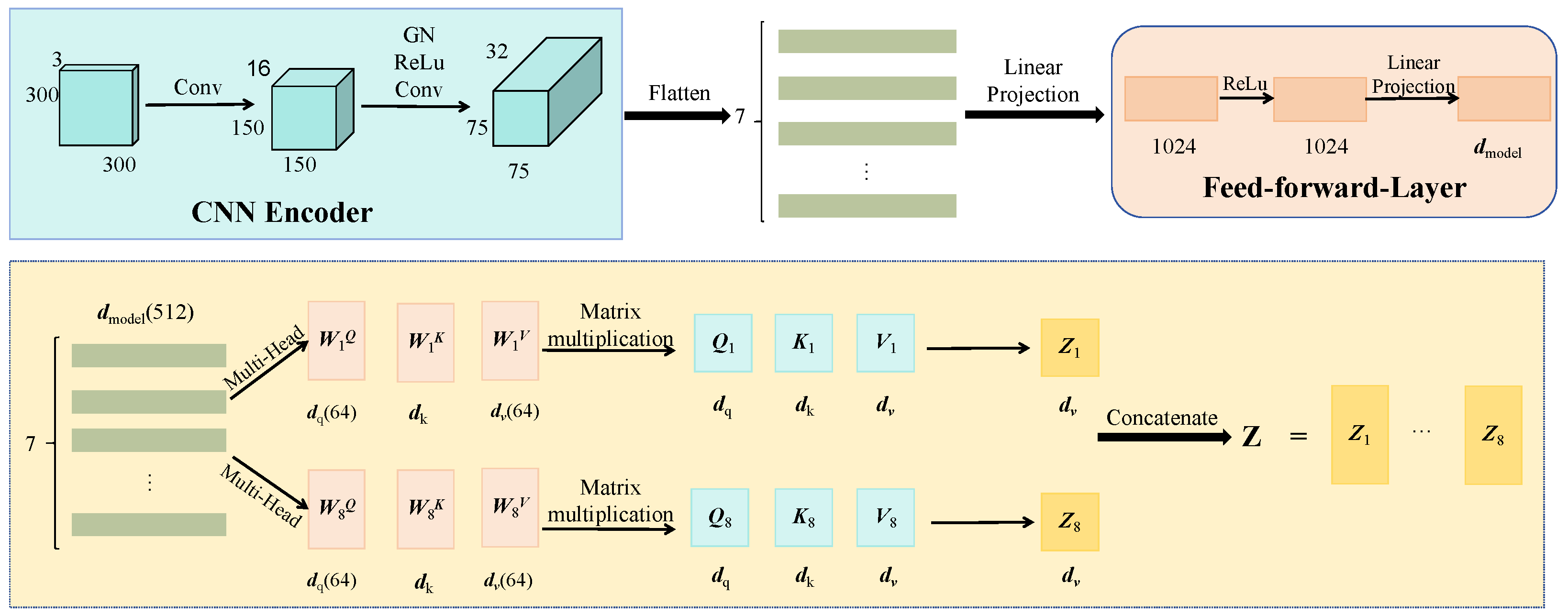
Figure 1. Overall architecture of the proposed hybrid model, including input embedding, attention mechanism, feed-forward layer, and multi-task prediction heads. The matrices W 1 Q , W 1 K , and W 1 V denote the linear projections for computing queries, keys, and values, respectively, with corresponding dimensions d q , d k , and d v . The feed-forward layer has an output dimensionality of 1024.
Information 16 00662 g001
Figure 2. Architecture of the Stability-Aware Scheduling Module based on the Actor–Critic framework. The Actor encodes real-time system states through linear layers and a GRU network to generate dispatch policies, while the Critic evaluates actions via soft Q-values. Expert demonstrations and replay buffers are integrated to enhance training stability and efficiency.
Information 16 00662 g002
Figure 3. Visualization of forecasting performance comparison.
Information 16 00662 g003
Figure 4. Training loss curves of different models over 200 epochs.
Information 16 00662 g004
Figure 5. Comparison of total operating cost and CCT across different models.
Information 16 00662 g005
Figure 6. Boxplot comparison of different models based on MAPE.
Information 16 00662 g006
Figure 7. Frequency deviation (Hz) comparison.
Information 16 00662 g007
Table 1. Multi-source data collection statistics for the power system.
Data TypeSourceNumber of VariablesNumber of Samples
Load powerGrid control systemresidential/industrial/commercial96k
Wind generationNEA/SCADAwind speed, direction, pitch, output, etc.96k
Solar generationSCADA systemirradiance, temperature, power output, etc.96k
MeteorologicalCMA/AWStemperature, humidity, pressure, wind, etc.96k
Grid statusRTU (IEC-104 protocol)frequency, voltage, angle, margin, etc.96k
Dispatch instructionScheduling platformtype, duration, magnitude, etc.96k
Table 2. Forecasting performance comparison.
ModelMAE (↓)RMSE (↓)MAPE (%) (↓)
SVR14.8218.259.32
CNN12.4616.878.15
GRU10.5113.927.42
LSTM10.0313.377.08
Autoformer9.4112.766.95
Proposed8.2111.485.82
Table 3. Economic cost and stability performance comparison.
ModelTotal Cost (↓)Frequency Deviation (Hz) (↓)CCT (s) (↑)
SVR153.60.2381.93
CNN145.20.1942.06
GRU141.80.1762.13
LSTM139.40.1692.20
Autoformer136.20.1582.35
Proposed128.30.1292.74
Table 4. Ablation study of key modules.
ConfigurationMAETotal CostFrequency Deviation (Hz)
w/o CNN Module10.74143.50.183
w/o LSTM Module11.26147.20.191
w/o Uncertainty Modeling9.85137.10.153
w/o Stability Scheduling9.02131.60.143
Full Model (Ours)8.21128.30.129
Table 5. Robustness evaluation on public SmartMeter dataset.
ModelMAE (↓)RMSE (↓)MAPE (%) (↓)
SVR15.0418.579.48
CNN12.8716.648.32
GRU10.7814.237.58
LSTM10.3213.627.24
Autoformer9.7413.056.91
RO (Two-stage)10.1213.346.78
SO (Two-stage)9.8712.966.52
Transformer9.4112.746.33
Galindo Transformer9.0212.236.01
MultiDeT8.8811.955.93
Proposed (Ours)8.4511.735.87
Disclaimer/Publisher’s Note: The statements, opinions and data contained in all publications are solely those of the individual author(s) and contributor(s) and not of MDPI and/or the editor(s). MDPI and/or the editor(s) disclaim responsibility for any injury to people or property resulting from any ideas, methods, instructions or products referred to in the content.