Ambiguities, Built-In Biases, and Flaws in Big Data Insight Extraction

Abstract

I address the challenge of extracting reliable insights from large datasets using a simplified model that illustrates how hierarchical classification can distort outcomes. The model consists of discrete pixels labeled red, blue, or white. Red and blue indicate distinct properties, while white represents unclassified or ambiguous data. A macro-color is assigned only if one color holds a strict majority among the pixels. Otherwise, the aggregate is labeled white, reflecting uncertainty. This setup mimics a percolation threshold at fifty percent. Assuming that directly accessing the various proportions from the data of colors is infeasible, I implement a hierarchical coarse-graining procedure. Elements (first pixels, then aggregates) are recursively grouped and reclassified via local majority rules, ultimately producing a single super-aggregate for which the color represents the inferred macro-property of the collection of pixels as a whole. Analytical results supported by simulations show that the process introduces additional white aggregates beyond white pixels, which could be present initially; these arise from groups lacking a clear majority, requiring arbitrary symmetry-breaking decisions to attribute a color to them. While each local resolution may appear minor and inconsequential, their repetitions introduce a growing systematic bias. Even with complete data, unavoidable asymmetries in local rules are shown to skew outcomes. This study highlights a critical limitation of recursive data reduction. Insight extraction is shaped not only by data quality but also by how local ambiguity is handled, resulting in built-in biases. Thus, the related flaws are not due to the data but to structural choices made during local aggregations. Although based on a simple model, these findings expose a high likelihood of inherent flaws in widely used hierarchical classification techniques.

1. Introduction

Collecting and treating huge masses of data has become an essential part of almost any activity, covering a rather large spectrum of fields. However, the related extraction of accurate and meaningful information from heterogeneous and diverse datasets may be delicate and sometimes misleading, with risks of information loss, bias outcomes, and misinterpretation. This issue represents a major challenge for data science.

Many common analytical techniques are available; yet, while these techniques are designed to extract inferences under uncertainty, each of them incorporates specific tradeoffs that can significantly affect the feasibility of the insights obtained.

For instance, Principal Component Analysis (PCA) is a widely used technique for dimensionality reduction, transforming high-dimensional data into a lower-dimensional space that captures the greatest variance [1]. However, PCA assumes linear relationships and can obscure localized or nonlinear structures. Similarly, t-distributed Stochastic Neighbor Embedding (t-SNE) is a nonlinear technique effective for visualizing aggregates, but is highly sensitive to parameter choices and does not preserve global distances well [2].

On the other hand, aggregating algorithms such as k-means and DBSCAN (Density-Based Spatial Aggregating of Applications with Noise) aim to partition data into meaningful groups. While k-means minimizes intra-aggregate variance assuming spherical aggregates of similar size, DBSCAN identifies aggregates based on density connectivity and can detect arbitrarily shaped aggregates [3]. However, both methods require careful parameter tuning and can struggle with noisy or unbalanced data.

In addition, when multi-scale data are involved, as in statistical physics and image analysis, coarse-graining methods are very efficient in extracting insights [4]. These methods can handle large-scale data; yet, ambiguity resolution and information compression introduce the potential for distortion at each stage of aggregation, especially when uncertainty is ignored or oversimplified [5].

All of these methodological issues become particularly critical in classification tasks, where simplified representations must still support accurate decision-making. Among a series of potential flaws, small distortions can cascade into systematic misclassifications.

Indeed, research into algorithmic fairness and explainable machine learning has shown that oversights in preprocessing or model design can have epistemic and ethical consequences [6]. Therefore, extracting insights from a dataset is not merely a technical process but a conceptual one, requiring scrutiny of the assumptions baked into every transformation, aggregation, and inference [7,8].

I previously demonstrated this point in an idealized case involving identification of a would-be terrorist from a large set of data obtained by monitoring a suspicious person. By labeling each ground item as Terrorist-Connected or Terrorist-Free, coarse-graining of all collected ground items is implemented to end up eventually labeling the person under scrutiny as a would-be terrorist or not a would-be terrorist [9,10]. The results showed the existence of systematic wrong labeling for some specific ranges of the item proportions. In particular, the flaw proves to be irremovable due to its being anchored within the treatment of uncertain aggregates of items which appear inevitably.

In this paper, I extend the above illustration to a more general setting by addressing the challenge of extracting reliable macroscopic information from non-annotated microscopic data. To that end, I investigate a stylized model that determines the macro-color of a collection of individually colored pixels using a repeated coarse-graining process based on bottom-up hierarchical aggregation. Here, the collection of colored pixels is an idealization of big data. Each pixel is assigned one of three colors, red, blue, or white. Red and blue serve as illustrative categories that can represent any form of underlying content or classification such as traits, behaviors, or detection statuses, depending on the application; in contrast, white denotes an unclassified or undecided state.

The process begins by forming groups of r randomly selected pixels. The color of each aggregate is then determined by applying a local majority rule. The procedure is repeated across successive layers, with each new layer formed by grouping r aggregates from the layer below and assigning their color using the same local majority rule. As the hierarchical structure develops, the system ultimately converges to a final super-aggregate encompassing all pixels. The resulting macro-color provides the final classification of the entire collection. When more than fifty percent of the pixels are red or blue, the corresponding macro-color is expected to be red or blue, respectively; otherwise, it is considered white.

By fixing all aggregates to size $r=4$, it is possible to solve the model analytically; in addition, I complement the analysis with simulations. While the hierarchical scheme is intuitive and computationally efficient, the results reveal that it produces misleading outcomes. The repeated application of local majority rules introduces cumulative information loss, which becomes increasingly pronounced at higher levels of aggregation. In particular, early ambiguities caused by possible white pixels and tie groupings propagate upward;,through repeated filtering, these always distort the final result for some specific range of the respective proportions of pixel colors. As a consequence, the system frequently converges to a macro-color that does not accurately represent the original proportions of red and blue pixels.

This distortion is not the product of randomness or local fluctuations, but rather stems from structural limitations inherent in the coarse-graining process. The recursive majority rule acts as a nonlinear filter, suppressing white aggregates and amplifying early local biases. Even very few white aggregates in the initial layers can disproportionately affect the outcome, leading to systematic misclassification. By analyzing how such distortions emerge and accumulate, the results expose the subtle but significant flaws embedded in hierarchical aggregation methods commonly employed in data reduction and classification tasks.

Last but not least, it is worth noting that similar phenomena occur in opinion dynamics with the democratic spreading of minorities, which take advantage of doubts and prejudices to convince an initial majority to shift opinion [11]. The thwarting of rational choices is also active in financial markets [12]. These works subscribe to the active field of the modeling of opinion dynamics within the field of sociophysics [13,14,15,16,17,18,19,20,21,22,23,24,25,26,27].

Outline of the Paper

The remainder of the paper is organized as follows. In Section 2, I define the hierarchical coarse-graining procedure in precise terms and introduce the majority rule dynamics governing color assignment at each level. Analytical tools are employed to characterize the evolution of color distributions through successive layers of aggregation, with special focus on the case where $r=4$.

An exact analytical solution is derived for the setting in which only blue (B) and red (R) pixels are present. The use of repeated local aggregations is shown to already produce indecisive aggregates at the first level of the hierarchy. In cases of ties, aggregate are labeled B with probability k and R with probability $(1-k)$. The repeated appearance of local ambiguities with related symmetry-breaking can drive the spread of the minority pixel color while climbing the hierarchy.

The impact of including a third color (white) is studied in Section 3. Exact analytical solutions demonstrate how local ambiguities propagate through the formation of white aggregates. I provide a detailed examination of the nonlinear filtering effect induced by repeated majority decisions and its consequences for the final macro-color classification.

In Section 4, I build out the full flow of colors leading to the macro-color for a series of different sets of parameter values.

Section 5 reports the results of numerical simulations that complement the theoretical analysis. These simulations explore the probability of correct classifications under varying initial conditions, such as different proportions of red, blue, and white pixels. In addition, the simulations quantify how small local fluctuations can lead to large-scale misclassifications.

Finally, a short discussion is provided in Section 6; in particular, I emphasize the major impact of local decision rules during coarse-graining that introduce hidden biases. Understanding these structural flaws is critical for designing more robust and interpretable data aggregation procedures.

2. Majority Rule and Ambiguity for Two-Color Pixels

In this section, I define the hierarchical coarse-graining procedure given a collection of individually colored pixels with respectively red (R) and blue (B) colors in proportions $p_0$ and $(1-p_0)$.

All pixels are then distributed randomly in groups of four, yielding $2^4=16$ different types of configuration. Among them, two are single-colored, eight are composed by three pixels of the same color, and six involve a tie with two R and two B pixels. These sixteen configurations reduce to five in terms of different compositions of R and B.

Applying a majority rule to the first ten configurations yields five configurations where all pixels are replaced with R pixels and five where all are replaced with B pixels. The last six tied configurations are undetermined based on the majority rule, and require a special handling. To cover all possible treatments of a tie configuration, I introduce the parameter k, which provides the probability that 2R 2B → 4R and → 4B with probability $(1-k)$.

Each single-colored group is now turned to one aggregate of level one with the group color. The probability of having a level one R aggregate is

$$p_1=p_0^4+4p_0^3(1-p_0)+6k{p}_0^2{(1-p_0)}^2.$$

(1)

Repeating the procedure to build aggregates of level $2,3,\dots ,n$, where the last level n encompasses the full collection of pixels, leads to $p_0\to p_1\to p_2\to \dots \to p_{n-1}\to p_n$. For a collection of N pixels, the number n of successive coarse-grained iterations is provided by

$$n=⌊{\displaystyle \frac{lnN}{ln4}}⌋,$$

(2)

where the floor function ensures an integer value for the number n of hierarchical levels. As a side effect, when $N>4^n$, a number $N-4^n$ of pixels must be discarded.

The logarithmic dependence on N indicates that collecting larger numbers of items does not require a significant increase in the number of required iterations in order to treat the corresponding collection of pixels. For instance, going from $N=4096$ to $N=16,384$, i.e., adding 12,288 pixels, requires only one additional coarse-graining, with $n=7$ instead of $n=6$. To go up to $N=65,536$ pixels requires $n=8$, and only $n=10$ is required to process the huge number $N=1.04858{10}^6$.

To determine the dynamics driven by iterating Equation (1), I solve the fixed point Equation $p_1=p_0$ to obtain the values which are invariant under coarse-graining. Three fixed points are obtained, with $p_R=1$, $p_B=0$ being attractors and

$$p_{c,k}={\displaystyle \frac{(1-6k)+\sqrt{13-36k+36k^2}}{6(1-2k)}}$$

(3)

a tipping point between them. With $p_{c,0}={\displaystyle \frac{1+\sqrt{13}}{6}}\approx 0.77$, $p_{c,1/2}={\displaystyle \frac{1}{2}}$, and $p_{c,1}={\displaystyle \frac{5-\sqrt{13}}{6}}\approx 0.23$, I obtain ${\displaystyle \frac{1}{2}}\le p_{c,k}\le 0.77$ for $0\le k\le {\displaystyle \frac{1}{2}}$ and $0.23\le p_{c,k}\le {\displaystyle \frac{1}{2}}$ for ${\displaystyle \frac{1}{2}}\le k\le 1$.

At this stage it is worth stressing that obtaining the level-n aggregate does not guarantee reaching one of the two attractors with $p_n\ne p_R\&p_B$. In such a case, the color labeling is probabilistic: R with probability $p_n$, and B with probability $(1-p_n)$.

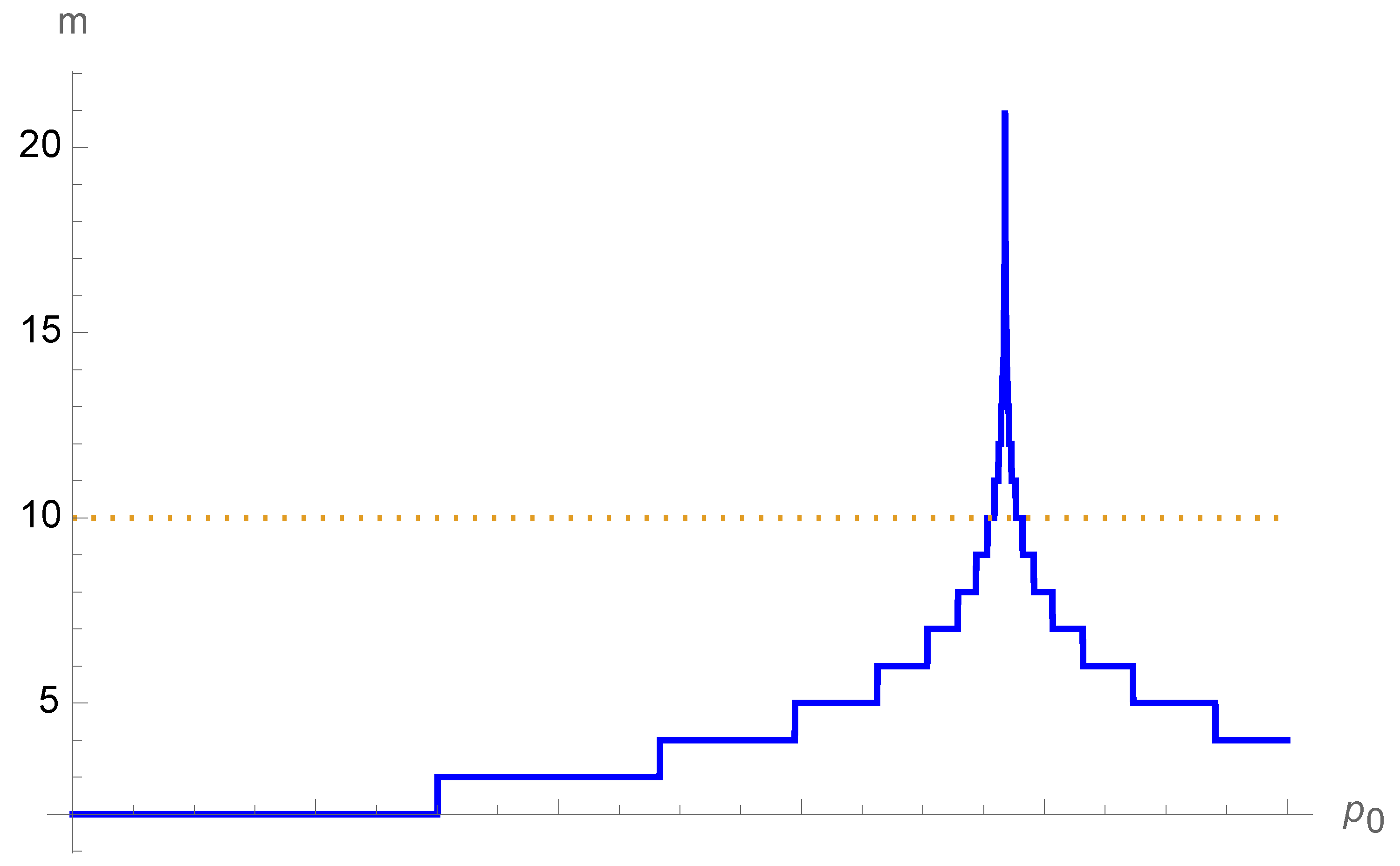
Starting from a proportion $p_0$ of R pixels, ensuring that it is possible to reach one of the two attractors requires a number

$$m=⌊{\displaystyle \frac{1}{ln{\lambda }_k}}ln{\displaystyle \frac{1}{|1-\frac{p_0}{p_{c,k}}|}}⌋+2$$

(4)

of hierarchical levels [28], where ${\lambda }_k\equiv {\displaystyle \frac{d{p}_1}{d{p}_0}}{|}_{p_{c,k}}$ with ${\lambda }_0={\lambda }_1\approx 1.64$ and ${\lambda }_{{\displaystyle \frac{1}{2}}}={\displaystyle \frac{3}{2}}$.

While Equation (4) is an approximation [28], it yields exact results for most cases. Most of the associated values are less than 10, as seen from Figure 1 for $k=0$. Only in the immediate vicinity of the tipping point $p_{c,0}\approx 0.77$ does m exhibit a cusp around 20. There, $N=4^{20}$ pixels are required to reach the attractor, which is often out of reach (Equation (2)). Therefore, given $p_0$, a minimum number $N=4^m$ pixels is required, otherwise the color labeling becomes probabilistic.

Applying local majority rules to even-size groups naturally introduces the challenge of dealing with ambiguities in extracting information. These ambiguities appear naturally when a local tie occurs randomly with the same number of R and B pixels. In an aggregate of two R and two B pixels, there is no majority with which it is possible to identify the aggregate color, which in turn creates ambiguity in how to color the related aggregate. Thus, a decision has to be made in order to select one of the two colors.

Combining the above results with the conditions $p_0>0.50\Rightarrow$ macro-R (red) and $p_0<0.50\Rightarrow$ macro-B (blue) proves a systematic error with a wrong macro-color in either of the two following cases:

When $0\le k\le {\displaystyle \frac{1}{2}}$, the range ${\displaystyle \frac{1}{2}}\le p_0\le p_{c,k}$ yields a macro-B result, while the exact color is macro-R.

Similarly, when ${\displaystyle \frac{1}{2}}\le k\le 1$, the range $p_{c,k}\le p_0\le {\displaystyle \frac{1}{2}}$ yields a macro-R result, while the exact color is macro-B.

While these local wrong outcomes are meaningless per se, they are found to end up disrupting drastically the expected final outcome in terms of the actual macro-color of the collection of pixels.

These different scenarios can be illustrated by the case of tagging a person under scrutiny as a would-be terrorist [9]. Red pixels are associated with data which are terrorist-connected, while blue pixels represent terrorism-free data; thus, a macro-red color signals a would-be terrorist, while a macro-blue color means the person is not a would-be terrorist.

In the event of a tie, if the presumption of innocence prevails ($k=0$), then a systematic error occurs for all persons whose scrutiny has yielded a proportion of terrorist-compatible ground items (R) between $50\%$ and $77\%$. While these persons should be labeled would-be terrorists, as shown in the top part of Figure, they are instead wrongly labeled as not would-be-terrorists Figure 2.

In contrast, applying a presumption of guilt ($k=1$) in the event of a tie ensures that no would-be terrorists will be missed. However, the concomitant price is that all persons with more than $23\%$ but less than $50\%$ of terrorist-connected ground items (R) will be wrongly tagged as would-be terrorists when in fact they are not, as seen in the lower part of Figure 2.

3. Adding a White Third Color for Uninformative Items

In the above two-color case, an ambiguous aggregate is assigned a property by coloring it either R or B depending on the current expectation of the monitoring of the actual extraction of information. However, to cover a larger spectrum of cases, it is of interest to introduce a third color denoted white (W) to account for uninformative items resulting from unclassified or ambiguous states, which serves as a proxy for incomplete, missing, or uncertain data. White pixels can be present; even if they are not, however, W aggregates inevitably appear in the treatment of aggregates for which there exists no majority (either R, B, or W).

Thus, the problem becomes a three-color (R, B, W) problem in which applying a majority rule to groups of four items generates unsolved configurations for which no color is a majority. Nonetheless, a decision has to be made for each type of ambiguous configurations. The respective proportions of R, B, and W pixels are respectively $p_0,q_0,(1-p_0-q_0)$.

Distributing them randomly in groups of four can result in $3^4=81$ different configurations, of which fifteen have different compositions of R, B, and W. Accounting for the permutations in the respective configurations yields three with same color for the four pixels and 24 with the same color for three pixels. Applying majority rule to these nine configurations yields nine single-colored configurations, as follows:

• RRRR (1), RRRB (4), RRRW (4) ⇒ RRRR
• BBBB (1), RBBB (4), BBBW (4) ⇒ BBBB
• WWWW (1), WWWR (4), WWWB (4) ⇒ WWWW

where the numbers in parentheses are the numbers of equivalent configurations.

For the remaining six configurations, no color has the majority (i.e., three or more); accordingly, these configurations require special handling in order to decide which color to attribute to each of them.

The “synthesizer” must then select a series of criteria to allow for treatment of all cases. The associated rules can be directly related to a preconceived view on how to complete incomplete data or can a random selection in tune with the framework culture of the system operating the data.

This does not demonstrate a lack of rigor; on the contrary, searching for insights necessitates some a priori expectation. This motivation does not reverse the synthesis when it is clear (here, in the presence of a local majority); however, when in doubt (here, in the event of a tie) this local a priori expectation will make the difference one way or the other. An agent or IA sticks to the data when it is clear; in presence of uncertainty, however, some a priori expectation is inevitably at work. This could be unconscious or conscious, and is generally dictated by the corporate culture, for instance, and not by a conscious desire to manipulate the data.

While the absence of a majority in a group of four with only two colors is self-evident, the situation is richer in the case of three colors, as absolute and relative majorities are now possible. In addition, the white color is without identified content, meaning that its relative weight is not equal to those of red and blue.

Accordingly, with W not counting, for a strong relative majority of 2 R (B) against 0 B (R), I take WWWW with a probability u and $(1-u)$ for RRRR (BBBB). For a weak relative majority of 2 R (B) against 1 B (R), I take WWWW with a probability v and $(1-v)$ for RRRR (BBBB). In a tie between R and B (2, 2; 1, 1), I choose RRRR with probability r, BBBB with probability b, and WWWW with probability $(1-r-b)$. The following update rules apply to ambiguous configurations:

• RRWW ⇒ WWWW, RRRR with respective probabilities $u,(1-u)$
• BBWW ⇒ WWWW, BBBB with respective probabilities $u,(1-u)$
• RRBW ⇒ WWWW, RRRR with respective probabilities $v,(1-v)$
• RBBW ⇒ WWWW, BBBB with respective probabilities $v,(1-v)$
• RRBB, RBWW ⇒ RRRR, BBBB, WWWW with respective probabilities $r,b,(1-r-b)$.

Indeed, accounting for all different cases would require doubling the numbers of parameters from 5 to 10. Here, I have chosen to restrict the investigation to the five parameters shown in

Table 1. Update rules with multi-line probabilistic outputs with $t_1=$ for B, $t_2=$ for R, and $t_3=$ for W. The numbers in parentheses signal the numbers of equivalent configurations obtained by permuting the colors. The letters in parentheses are the probabilities of the respective outcomes of the updates.

Inputs	Outputs	Condition
BBBB (1), BBBR (4), BBBW (4)	BBBB	$t_1>2$
RRRR (1), RRRB (4), RRRW (4)	RRRR	$t_2>2$
WWWW (1), WWWB (4), WWWR (4)	WWWW	$t_3>2$
BBWW(6)	WWWW (u)
BBBB ($1-u$)	$t_1=t_3=2$
RRWW(6)	WWWW (u)
RRRR ($1-u$)	$t_2=t_3=2$
BBRW(12)	WWWW (v)
BBBB ($1-v$)	$t_2=t_3=1$
RRBW(12)	WWWW (v)
RRRR ($1-v$)	$t_1=t_3=1$
BBRR (6), BRWW(12)	BBBB (b)
RRRR (r)
WWWW ($1-b-r$)	$t_1=t_2=2,1$

in order to keep it focused and clear without losing generality. Given this choice, the update equations for a single coarse-grained iteration from level-n to level-(n + 1), I write

$$\begin{array}{cc}\hfill p_{n+1}& =p_n^2\left[p_n^2+4p_n{q}_n+4p_n(1-p_n-q_n)+6{(1-p_n-q_n)}^2(1-u)\right.\hfill \\ \hfill & \left.+12q_n(1-p_n-q_n)(1-v)\right]+b(6p^2{q}^2+12pq{(1-p-q)}^2),\hfill \end{array}$$

(5)

$$\begin{array}{cc}\hfill q_{n+1}& =q_n^2\left[q_n^2+4p_n{q}_n+4q_n(1-p_n-q_n)+6{(1-p_n-q_n)}^2(1-u)\right.\hfill \\ \hfill & \left.+12p_n(1-p_n-q_n)(1-v)\right]+r(6p^2{q}^2+12pq{(1-p-q)}^2),\hfill \end{array}$$

(6)

with $(1-p_{n+1}-q_{n+1})$ yielding W for the aggregate.

Solving the associated fixed-point equations $p_{n+1}=p_n$ and $q_{n+1}=q_n$ generates a two-dimensional landscape for the dynamics of opinion, instead of the previous one-dimensional landscape with only R and B. Analytical solving is no longer feasible, and a numerical treatment must be used instead.

4. Results from the Update Equations

My main focus in this work is not to discuss the nature and merits of each choice of treatment of the various ambiguities implemented by $(u,v,r,b)$, but rather to demonstrate that the appearance of ambiguities is inevitable from the coarse-graining process and that some pixel compositions $(p,q)$ will result in erroneous macro-color diagnoses irrespective of how they are sorted.

On this basis, with the parameter space having six dimensions $(p,q,u,v,r,b)$, I restrict the investigation to a series of representative cases without losing generality. The underlying surface of expected exact macro-colors is exhibited in Figure 3 as a function of distributions of p and q. The light blue, red, and white triangles delimit the areas with a majority of pixels, respectively B, R, and W. There, the exact macro-colors are B, R, and W. In the central green triangle, no absolute majority (more than half) prevails; however $p+q>0.50$ with a relative majority of one of the two colors in relation to the other. Thus, some arbitrage is required to set the related expected macro-color, if any.

For each set of chosen parameters $(u,v,r,b)$, I identify all associated fixed points using Equations (5) and (6) together with their respective stabilities. I then build the related two-dimensional complete flow diagram generated by the coarse-graining from every point $(p,q)$ until its ending attractor. Stable, unstable, and saddle fixed points are shown in the figures by blue, red and magenta, respectively.

The obtained diagram indicates areas of pixel composition ending in wrong macro-color outcomes. As can be seen from Table 1, I consider a symmetry of B and R against W, using u for both BBWW and RRWW configurations and v for both BBRW and RRBW. At this stage, including a B–R asymmetry would only blur the readability of the results. Assuming full symmetry between R and B implies that $r=b$.

It is worth emphasizing that $p+q<1$ implies a proportion $(1-p-q)$ of white pixels in the sample. In addition, white aggregates appear during the coarse-graining implementation as a function of the treatment of local ambiguities depending on the value of $(u,v,r,b)$. With this regard, for each $(u,v,r,b)$ set, I show two flow diagrams to discriminate the impact of white pixels from the forming of white aggregates. One includes the full two-dimensional triangular surface, which embodies any pixel composition $(p,q,1-p-q)$, while the other includes with samples with no white pixels, i.e., along the one-dimensional line $p+q=1$.

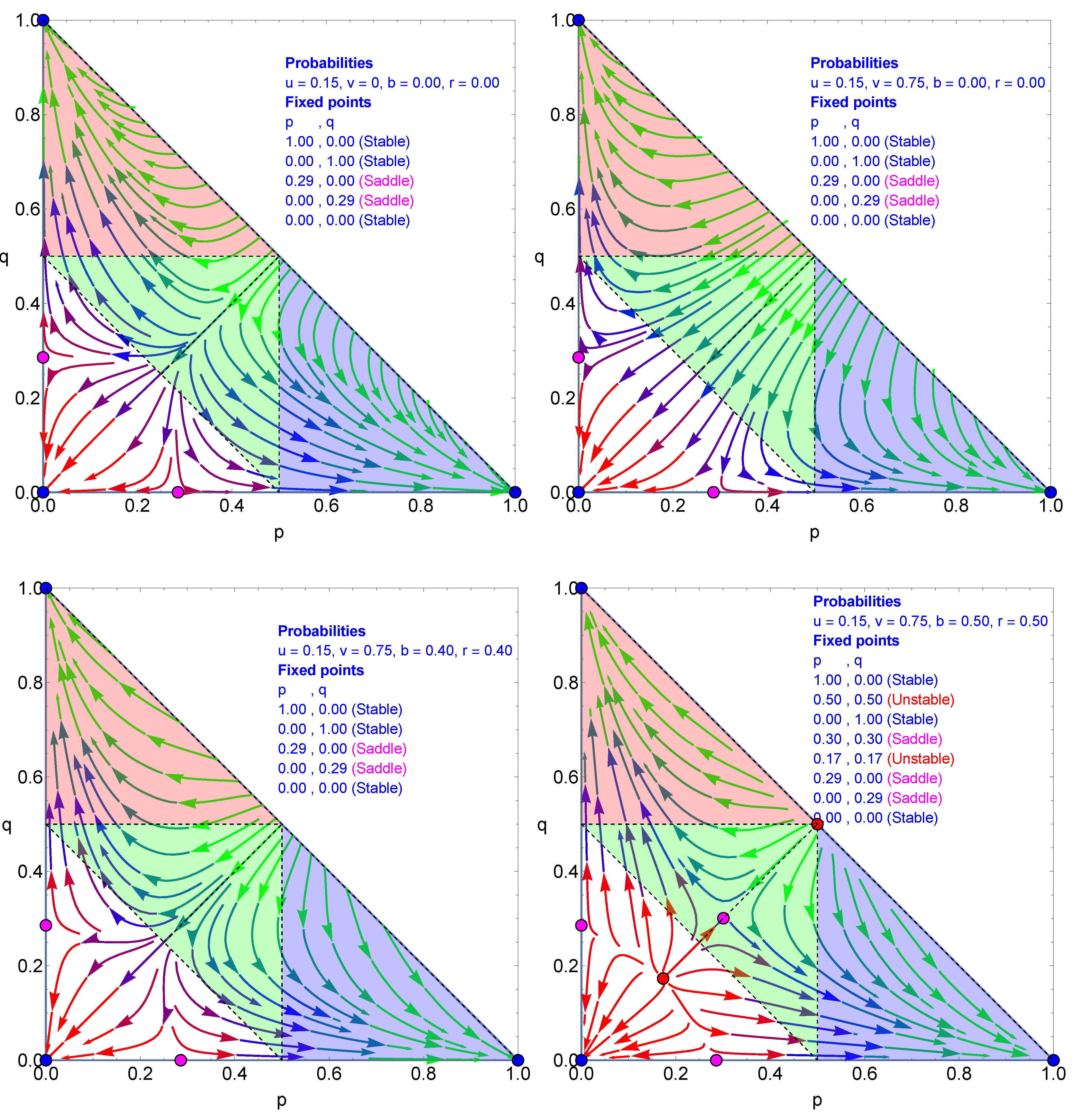
I start with W, not taken into account in the local calculations of the majority, i.e., $u=v=0$. Thus, W always disappears for WWWB and WWWR, which yields WWWW following the majority rule. If W does not count locally, then $b=r=0.50$, meaning that there is no tie-breaking effect. Seven fixed points are found, which are listed in the upper left part of Figure 4. The basin of attraction of the W attractor ($p=q=0$) is at its minimal area. The green area leads equally to B ($p=1,q=0$) and R ($p=0,q=1$) attractors.

When BBRR and BRWW yield WWWW with probability $(1-b-r)\ne 0$, then $b=r<0.50$. The case with $b=r=0.20$ is shown in the upper right part of Figure 4. Comparing with the upper left part indicates that the flows along the $q=0$ and $p=0$ lines are unchanged, with the tipping point still located at 0.23 for each. However, the two unstable and saddle fixed points ($p=q=0.12$) and ($p=q=0.50$) have moved toward each other, with $p=q=0.18$ and $p=q=0.42$.

With ($b=r=0$), the two unstable and saddle fixed points move to ($p=q=0.3$) and ($p=q=0.33$), but do not overlap, as seen in the lower left part of Figure 4. Only $u=0.01$ generates the overlap at ($p=q=0.32$), as shown in the lower right part of Figure 4. In addition, the tipping points on the axes move to 0.24.

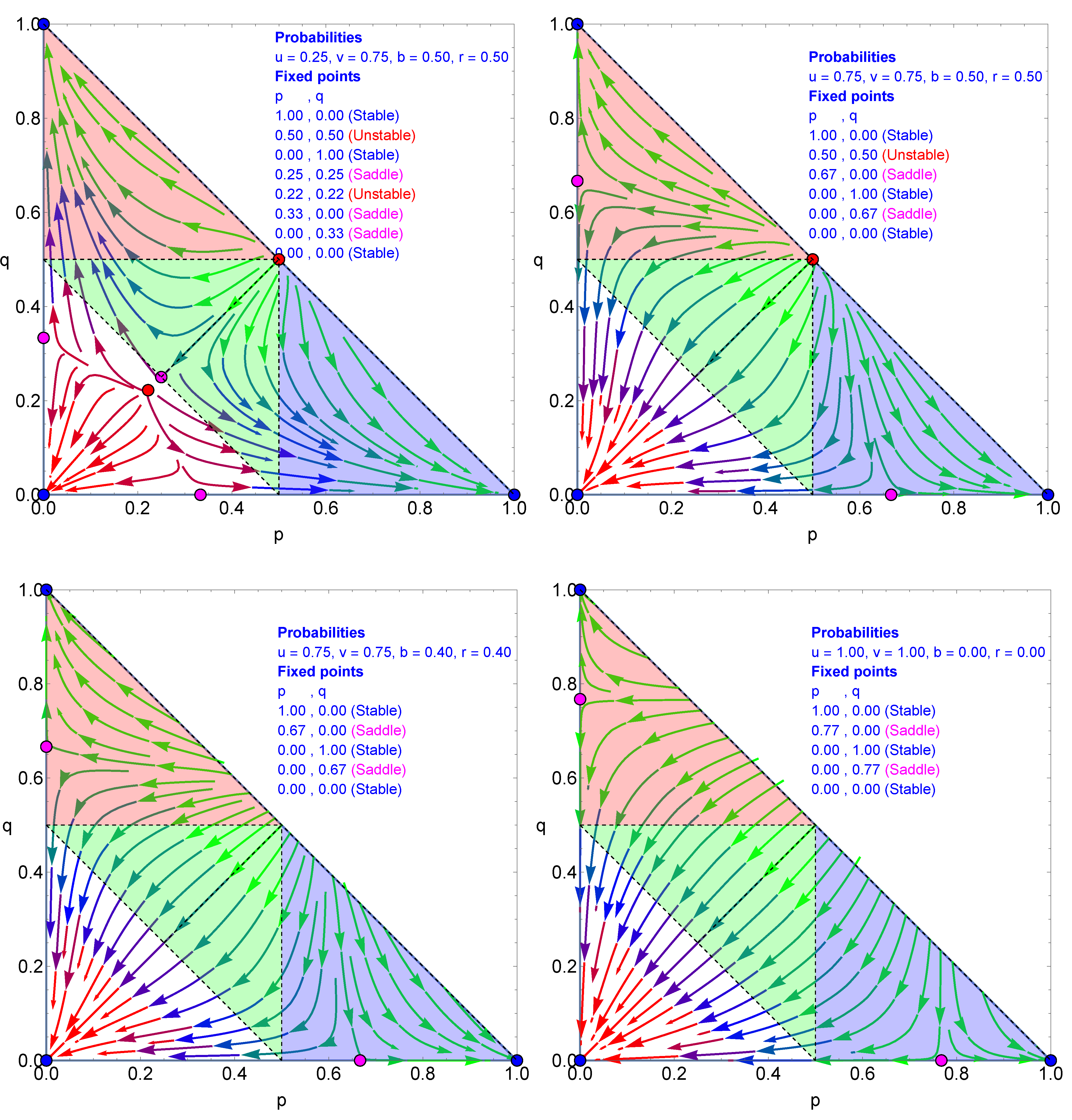
After coalescing, the fixed points ($p=q=0.32$) disappear, leaving the flow landscape driven by only five fixed points, as illustrated in the upper left part of Figure 5 for $u=0.15$. Moving to the case with $u=0.15,v=0.75,b=r=0$, there is little effect on the dynamics besides directing the flows more quickly toward the two attractors $(1,0),(0,1)$, as exhibited in the upper right part of Figure 5. Increasing $(b,r)$ from $(0,0)$ to $\left(0.40\right)$ does not have much effect, as shown in the lower left part of Figure 5; however, $(b=r=0.50)$ reintroduces three fixed points to reach a total of seven, as seen in the lower right part of Figure 5.

Increasing u from 0.15 to 0.25 while keeping $v=0.75,b=r=0.50$ unchanged has little effect. However, for $u=0.75)$, two fixed points disappear, leaving the dynamics driven by six fixed points, as respectively exhibited in the left and right sides of the upper part of Figure 6. The lower part of Figure 6 shows that while $(u=v=0.75,b=r=0.40)$ does not have much effect, $(u=v=1,b=r=0)$ shifts the axis attractors from 0.67 to 0.77.

All of the above cases highlight the unavoidable flaws produced by the handling of local ambiguities, with the way they are treated contributing in part to classification as B, R, and W.

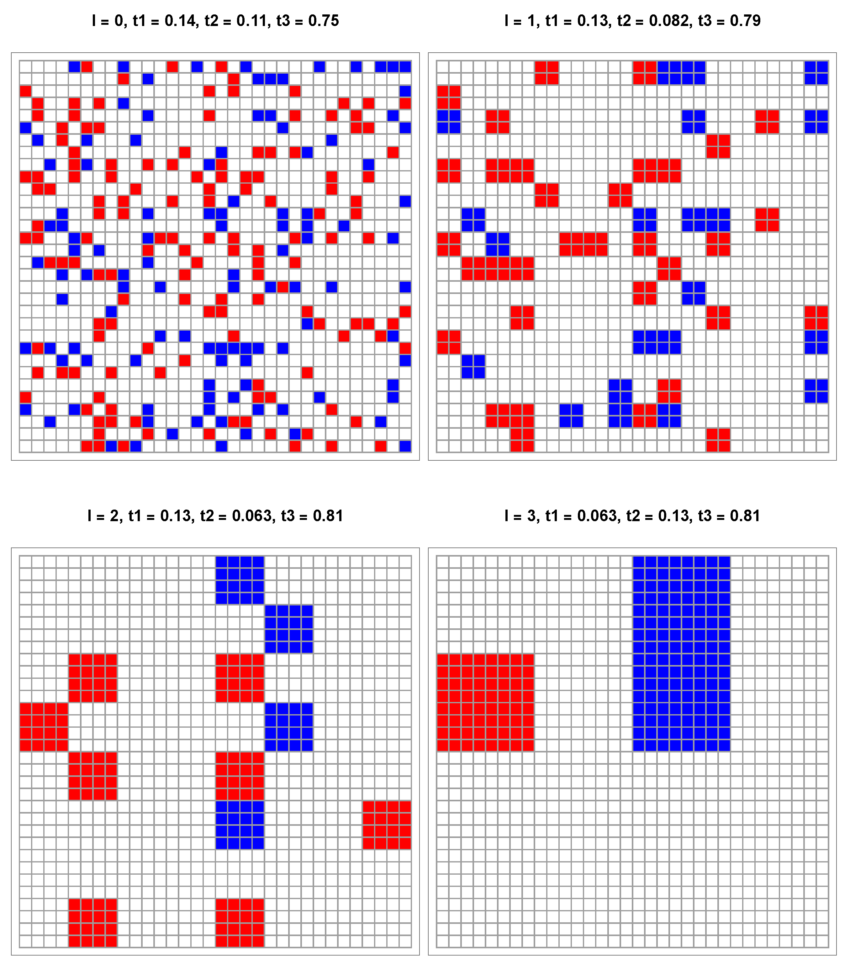
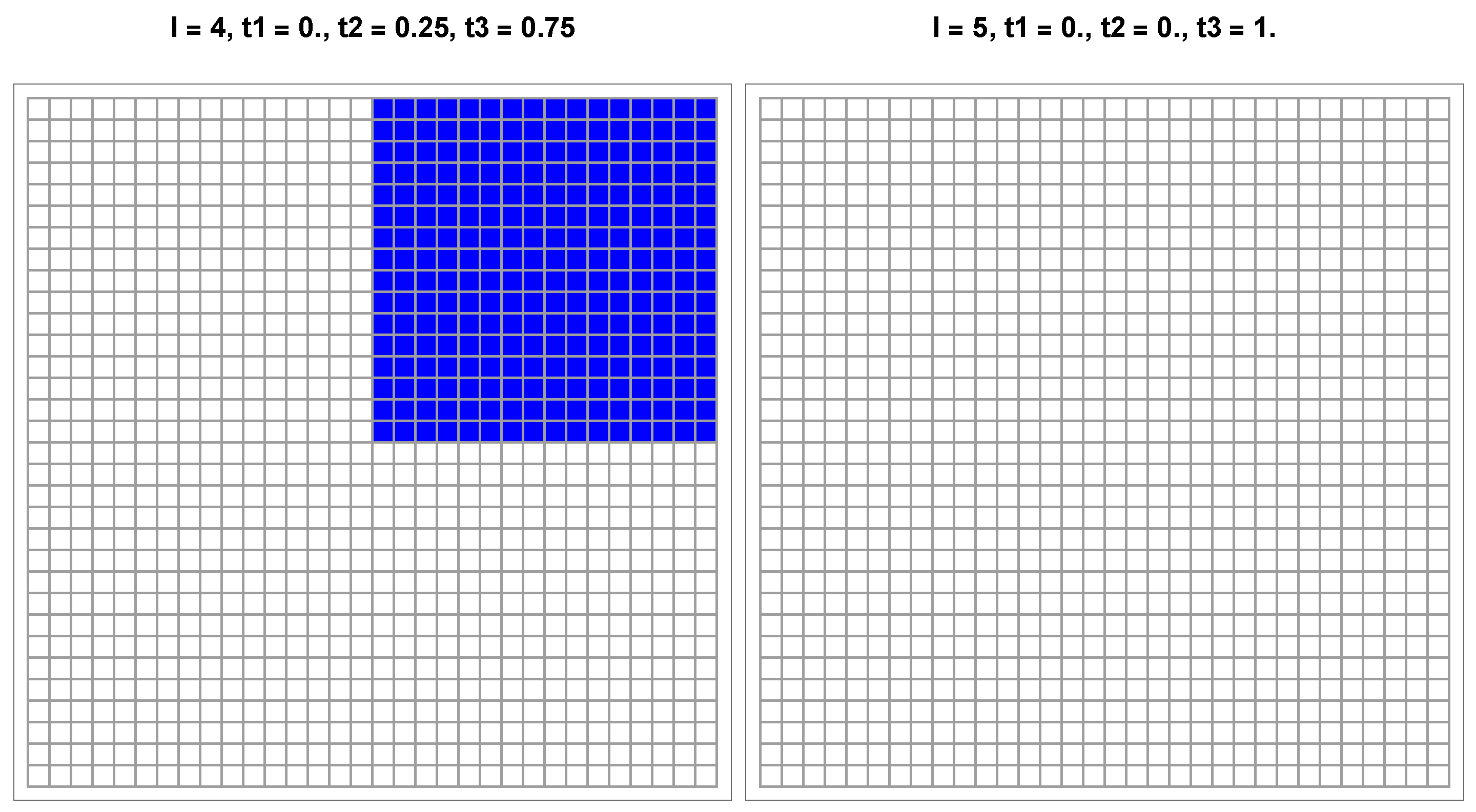
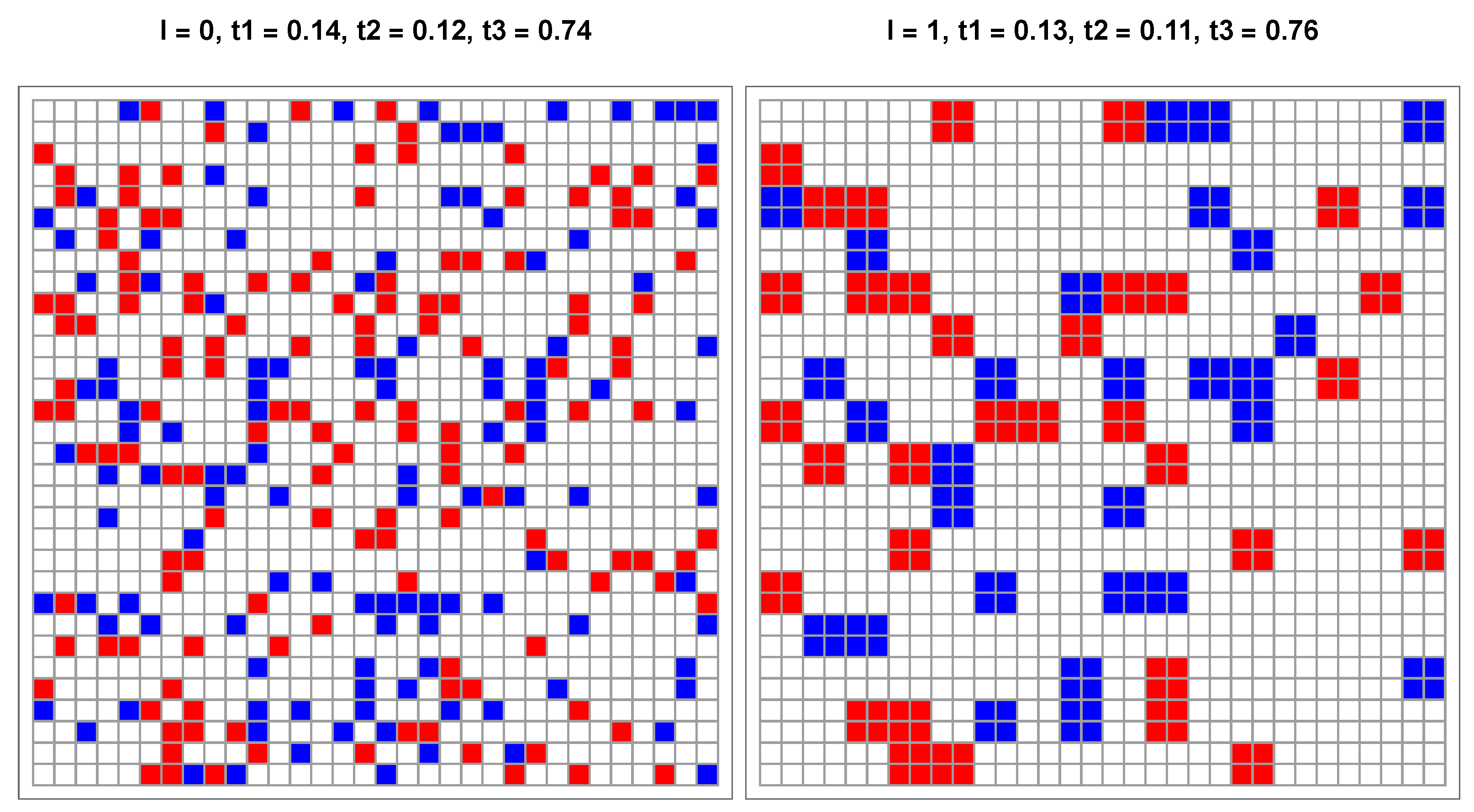
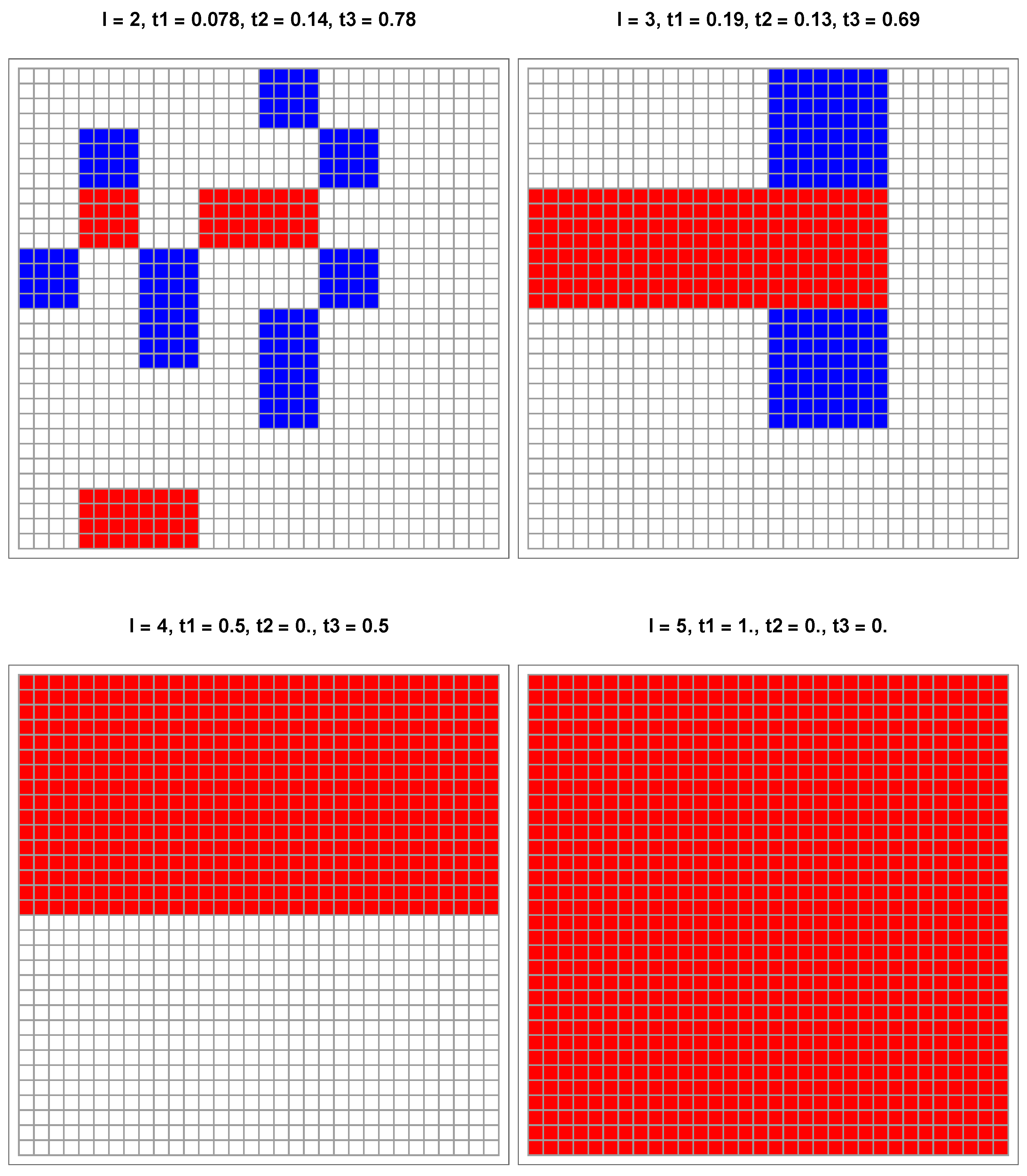
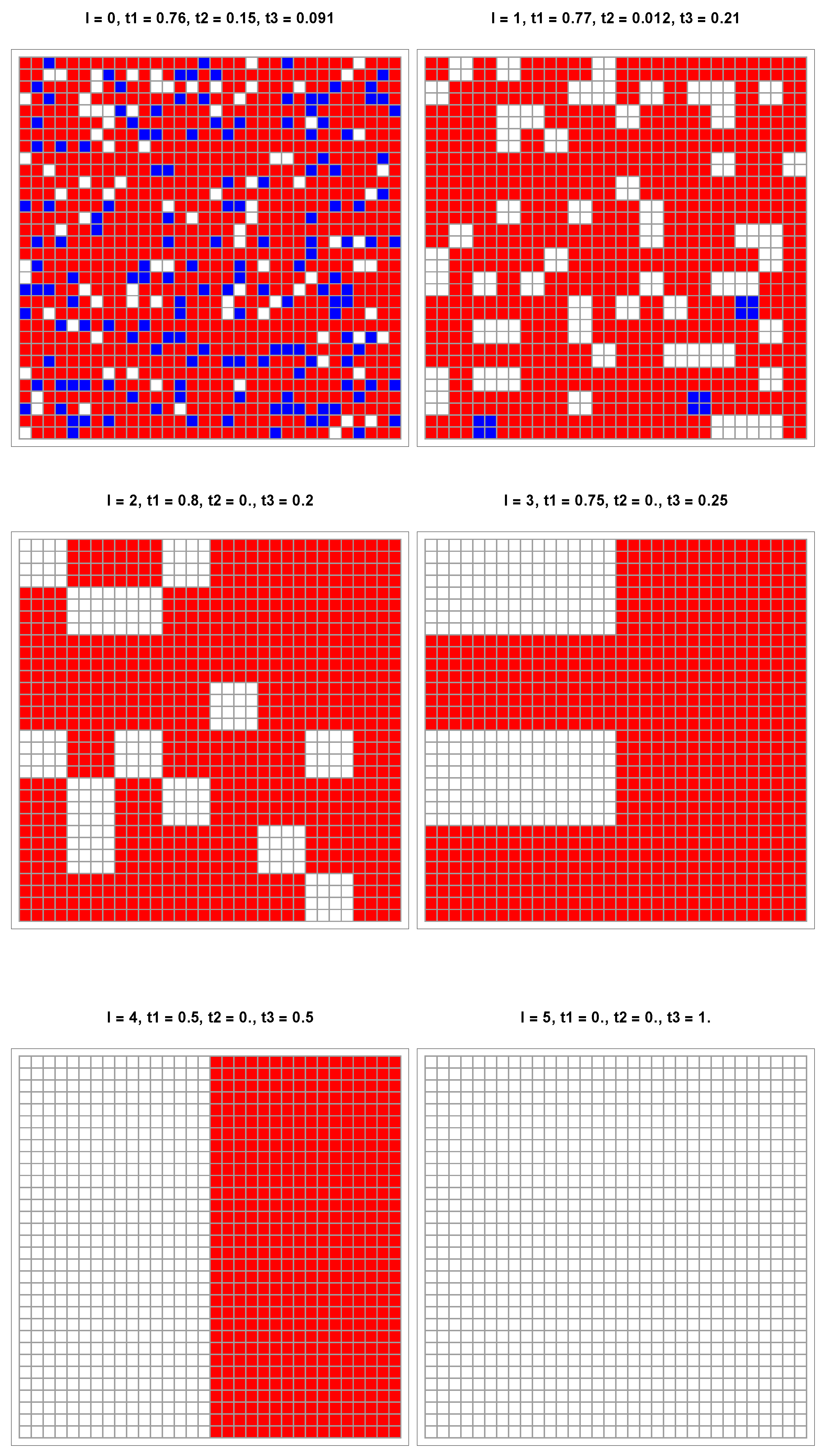
5. Results from Simulations

To validate the above results, I ran simulations to materialize the actual coarse-graining of a collection of colored pixels. Because one simulation is required for each pair $(p_0,q_0)$, I report only three cases here to illustrate the process. I treat collections of 1064 pixels randomly distributed on a $2^5\times 2^5=32\times 32$ grid, which corresponds to five consecutive updates. Each level of coarse-graining is numbered $l=1,2,3,4,5$, with $l=0$ for the actual collection of pixels. For each level l, $t_1,t_2,t_3$ denote the proportions of aggregates, respectively, blue, red, and white. The parameters $t_1,t_2,t_3,l$ are identical to $p_n,q_n,1-p_n-q_n,n$ used for the above update equations.

The first case is associated with point $t_1=0.14,t_2=0.11,t_3=0.75$ given $u=v=0$, $b=r=0.50$. The upper left part of Figure 4 lists the associated seven fixed points driving the dynamic flow. In particular, starting from $p_0=0.14,q_0=0.11$ leads to the W attractor $p_0=q_0=0$, which is the correct label for $75\%$ of W pixels. The related five levels are exhibited in Figure 7 with the same macro-color.

I note that $t_1=0.14,t_2=0.11$ is within the basin of attraction delimited by the unstable fixed point (0.12, 0.12) and the two saddle points at (0.23, 0) and (0, 0.23).

In the second case, I slightly shift the proportion of R to $t_1=0.14,t_2=0.12$, which is now outside the basin of attraction. As expected, the simulation shown in Figure 8 recovers a B macro-color from the upper left part of Figure 7. However, this final label is wrong, since both $p_0$ and $q_0$ are less than $50\%$.

The last case shown in Figure 9 has $u=v=1$, $b=r=0$ and $t_1=0.76,t_2=0.15$. While the exact macro-color is B, the coarse-graining wrongly yields W, similarly to the update equations, as seen in the lower right part of Figure 6. The reason for this is that the p axis has W and B attractors separated by a saddle fixed point located at 0.77.

The three simulations exhibited above recover the results yielded by the update equations, showing that further simulations are not needed at this stage.

6. Conclusions

To address the subtle challenge of extracting reliable insights from large datasets, I have explored the minimal yet illustrative case of a collection of colored pixels—red, blue, or white—for which the overall macro-color is defined by the actual majority color among the pixels. Assuming that the pixel color proportions are not directly accessible, I apply a recursive coarse-graining procedure to infer the macro-color from local configurations.

This approach frames the problem within the broader context of classification under uncertainty in big data. Each coarse-graining step acts as a local classifier operating with incomplete local information, specifically the appearance of aggregates without local majority, and the entire procedure forms a stacked ensemble of such decisions.

The analysis shows that recursive majority-vote rules frequently fail to recover the correct macro-color due to the unavoidable unclassified appearance of white aggregates. These ambiguous cases require arbitrary decisions in order to proceed. By systematically exploring the space of such decisions, I have identified the parameter regimes in which the process yields incorrect outcomes.

The central conclusion of this work is that inherent related biases propagate through the hierarchy regardless of the chosen local decision rules, which are inevitably required, leading to distortions in the final classification. In this sense, the coarse-graining process itself becomes a source of systematic error, even when starting from an unbiased configuration.

In particular, the results highlight how the mere presence of unclassified white aggregates misleads the inference of global properties, underlining the fragility of hierarchical procedures in the face of local ambiguities.

This study emphasizes that robust insight extraction depends not only on the volume of data but also on how local uncertainties are handled. Hierarchical aggregation schemes inherently act as symmetry-breaking mechanisms, whether through deterministic or stochastic rules, ultimately favoring one outcome over another.

Although these local instances of symmetry breaking may appear to be sound, minor, or inconsequential, their cumulative effect can be profound. As ambiguities propagate through the hierarchy, small asymmetries in rule design or data distribution can give rise to significant macroscopic biases, even in complete datasets.

Though based on a simple model, these findings offer insights into widely used data reduction techniques. In particular, they demonstrate that the impact of unintentional bias in hierarchical classification processes is unavoidable. Recognizing and addressing this practical flaw is crucial for extracting meaningful categorical insights from complex, multi-scale data.