New Permutation-Free Quantum Circuits for Implementing 3- and 4-Qubit Unitary Operations

Abstract

The article presents the quantum signal-induced heap transform (QsiHT) method of the QR-decomposition of multi-qubit operations. This transform can be generated by a given signal, by using different paths, or orders, of processing the data. We propose using the concept of the fast path of calculation of the QsiHT and applying such transforms on each stage of the matrix decomposition. This allows us to build quantum circuits for multi-qubit unitary operation without permutations. Unitary operations with real and complex matrices are considered. The cases of 3- and 4-qubit operations are described in detail with quantum circuits. These circuits use a maximum of 28 and 120 Givens rotation gates for 3- and 4-qubit real operations, respectively. All rotations are performing only on adjacent bit planes. For complex unitary operation, each of the Givens gates is used in pairs with two Z-rotation gates. These two types of rotations and the global phase gate are the universal gate set for multi-qubit operations. The presented approach can be used for implementing quantum circuits for $n$-qubits when $n\ge 2$, with a maximum of ($4^n/2-2^{n-1})$ Givens rotations and no permutations.

1. Introduction

In recent years, increased work has been done but much remains to be done in the development of existing and novel methods of data processing in new computers named quantum computers. Quantum circuits are complex, since all operations, or gates, should be invertible (unitary), and all calculations should be performed on normalized data, which are called quantum superpositions [1,2]. Another feature is the impossibility of measuring the quantum states during calculation in circuits without destroying the complete quantum superposition. Quantum states change instantly as soon as they are observed. In other words, they are well protected from our interference. So even simple tasks require hundreds of thousands of runs of the same quantum circuit to observe reliable data for computing. All that tells us that we need to develop effective and, most importantly, simple methods of building quantum circuits. Many simple one- and two-qubit gates are well known in quantum computation [3,4,5]. However, how to use them in the most effective way to build universal codes, or circuits, to compute multi-qubit quantum operations is still an open problem to be solved.

Multi-qubit operations, or gates, in quantum computation are described by unitary matrices, real or complex. It means that if we build the circuit for multi-qubit operation $A$, it is not difficult to obtain the circuit for inverse operation $A^{-1}$. This is a good and desirable property for the transform. However, the requirement for operation to be unitary makes it difficult to implement many important operations. For instance, in engineering, we mention the operation of linear convolution, correlation, linear filtration, optimal or Wiener filtration, and signal and image restoration [6,7].

Studying different methods of matrix decomposition, such as the Gramm–Schmidt process [8], the method of Householder transformations [9,10], cosine-sine decomposition (CSD) [11], and QR-decomposition by Givens rotations [12,13], we choose QR-decomposition. This decomposition, or the factorization for the case of unitary matrices, has been studied and used by many researchers. To build quantum circuits for multi-qubit operations and state preparations, this decomposition has been combined with different permutations [14,15,16,17,18,19,20]. The purpose of such additional permutations, including CNOT operations and Gray code-based permutations, is the requirement to fulfil the computations only on adjacent bit planes (BP), that is, which differ by only one bit [21,22,23]. The presence of permutations and CNOT gates is associated with multiple switching of information flows from one set of qubits to others. Even for a small number of qubits, for example, 4-qubit operations, the number of only CNOT operations is estimated as $100$. Many quantum circuits are populated with different switches. The possibility of removing all such permutations from the circuits was noted in our work devoted to 3-qubit operations [24]. Permutations are not mandatory elements in a universal set of gates, they are not needed at all for multi-qubit operations. We mention several quantum circuits that are used to compute the $n$-qubit quantum Fourier transform (QFT) [25,26]. It is a complicated operation, but implementation of this operation by the Cooley–Tookey algorithm [27,28] and paired-transform based method [29] do not include the CNOT gates in the circuits of the $n$-qubit QFT. In connection with what has been said, we present

Table 1. Number of CNOTs for $n$-qubit operation, when $n=2:7.$

$\mathit{n}$	$2$	$3$	$4$	$5$	$6$	7
QR [15]	4	64	536	4156	22,618	108,760
CSD [31]	8	48	224	980	3968	16,128
QSD (optimized) [30]	3	20	100	444	1868	7660
Lower bounds [32]	3	14	61	252	1020	4091
QR by QsiHT	0	0	0	0	0	0

with CNOT counts in the known circuits for $n$-qubit operations (see Table 1 in [30] (p. 1008)). This table includes for comparison, the known QR decomposition, cosine-sine decomposition (CSD), and quantum Shannon decomposition (QSD).

This work is the continuation of the above mentioned publication that describes in detail only the case of 3-qubit operations with real unitary matrices, not complex. Here, we consider the general case of 3- and 4-qubit operations. The QR-decomposition and circuits for computing these operations are described in detail. The QR-decomposition is based on the concept of the discrete-time signal-induced heap transform (DsiHT) [33,34]. Namely, we consider its particular case, when the transform is generated (induced) by one signal, not several. This transform is used in the QR decomposition with a special property. On each stage of the decomposition, we introduce the roadmap of the transform. It shows a path, the “fast path,” for the DsiHT to operate exclusively on adjacent bit-planes, which ensures optimization of the quantum circuit layout. That allows us to entirely eliminate CNOT gates and Gray-code permutations from the circuits.

The DsiHT is generated by a given signal, and there are many ways to compose this transform by using the path of the transform. The path is an especially important characteristic of the transform, and from the very beginning when this transform was presented (Grigoryan [35]), we have repeatedly drawn attention to the choice of this path. It was shown, for example, that the right choice of such a path may significantly reduce the number of zeros of the unitary matrix $Q$ in the decomposition $A=QR$ for a square matrix, in the general case when $A$ is not necessarily unitary. That reduces the number of multiplications in the matrix calculation. Thus, the traditional method of processing data in the natural order $0,1,2, \dots , (N-1$) is not the best way (or path) of processing data in QR decomposition of an $N\times N$ matrix $A$. In quantum computation, we only consider the case when $N$ is a power of 2, $N=2^r$. The quantum analogue of the $N$-point DsiHT is the $r$-qubit quantum signal-induced transform (QsiHT) [36].

The key contributions of this work are:

• New effective roadmaps or “fast paths” for all fifteen DsiHTs in the QR decomposition of a 4-qubit operation, real or complex. No additional permutations with Gray codes or CNOT gates are required in the decomposition.
• For any 3- or 4-qubit operation (circuit), the universal set of gates consists only of $Y$- and $Z$-rotations, plus the phase gate.
• For quantum operations with unitary real matrices, only Givens rotations are required.
• A universal and transparent circuit for quantum 3- and 4-qubit operations.
• The quantum circuit with a maximum of 120 controlled rotation gates and depth of 54 for 4-qubit real operation. The circuit for complex 4-qubit operation requires a maximum of $120$ $Y$-rotation gates, $240 Z$-rotation gates, and no permutations.
• A simple circuit for generating any 3- and 4-qubit operation with a real or complex unitary matrix by using an encoding table.
• A general method for constructing circuits for multi-qubit operations with maximum of $(4^n/2-2^{n-1})$ $Y$-rotation gates, $(4^n-2^n)$ $Z$-rotation gates and no permutations, for $n>1$ qubits.

The rest of the paper is organized as follows. In Section 2, the concept of the DsiHT is briefly discussed. The roadmaps for the 3-qubit QsiHT is presented. The complex DsiHT is considered in Section 3. Section 4 describes the method of DsiHT-based QR decomposition on the example with an 8 $\times$ 8 matrix, $A=QR$. In Section 5 and Section 6, the cases of 2- and 3-qubit quantum signal-induced heap transform (QsiHT) are considered in detail with two encoding tables and quantum circuits for complex 2- and 3-qubit operations. The quantum circuit of a 4-qubit unitary operation is presented in Section 7. All roadmaps for 15 QsiHTs in the QR-decompisition of the 4-qubit operation (complex and real) are presented in Appendix A.

2. The Concept of the DsiHT

The DsiHT is the unitary transformation that is induced, or generated, by one or more signals [37]. The illustration of this transform when the transform is generated by a single signal $\mathit{x}$ is shown in Figure 1. A signal-generator is shown in Figure 1a. The input and output of the generated transform are shown in Figure 1b and Figure 1c, respectively.

To compose such a transform, different ways of processing the components of the generator can be used. We consider the case when the transform is composed sequentially by the series of 2-point operations. At each stage of composition, only two components $x_n$ and $x_k$ of signal $\mathit{x}$ will be processed, for instance, the components number $n=3$ and $k=7$. These components can also be renewed during the calculations as well. By using these components, a 2-point operation, $T_{n,k}$, will be generated, and then, it will be applied on component number $n$ and $k$ of the input signal $\mathit{z}$, as shown in Figure 1. Thus, it is a two-level transformation. On the first level, the transforms $T_{n,k}$ are generated, and on the second level, they are applied on the input signal. Input signal $\mathit{z}$ can also be processed after generating the entire transform, DsiHT. We consider the simple case, when each 2-point transformation ${T=T}_{n,k}$ moves the energy of the input to one of its components. In other words, the transformation is defined as

$$T: \left(x,y\right)\to \left(\pm \sqrt{x^2+y^2},0\right)$$

(1)

or

$$T: \left(x,y\right)\to \left(0,\pm \sqrt{x^2+y^2}\right).$$

(2)

Here, the energy of the input $(x,y)$ is defined as $\sqrt{x^2+y^2}$ or $\sqrt{{|x|}^2+|{y|}^2}$ for the complex input.

First, we consider real transformations defined by the Given rotation, $T=R_{\vartheta }$, which is described in the matrix form as

$$R_{\vartheta }\left[\begin{array}{c}x\\ y\end{array}\right]=\left[\begin{array}{cc}\cos \vartheta & -\sin \vartheta \\ \sin \vartheta & \cos \vartheta \end{array}\right]\left[\begin{array}{c}x\\ y\end{array}\right]=\left[\begin{array}{c}\pm \sqrt{x^2+y^2}\\ 0\end{array}\right].$$

(3)

The angle is calculated by $\vartheta =-\arctan \left(y/x\right)$, and $\vartheta =\pm \pi /2$ if $x=0$. The transformation in Equation (2) is described by

$$R_{\vartheta }\left[\begin{array}{c}x\\ y\end{array}\right]=\left[\begin{array}{cc}\cos \vartheta & -\sin \vartheta \\ \sin \vartheta & \cos \vartheta \end{array}\right]\left[\begin{array}{c}x\\ y\end{array}\right]=\left[\begin{array}{c}0\\ \pm \sqrt{x^2+y^2}\end{array}\right],\hspace{1em}\hspace{1em}\vartheta =\mathrm{atan}{\displaystyle \frac{x}{y}}.$$

(4)

Because of the property $\mathit{atan}(x/y)$ + $\mathit{atan}(y/x)=\pi /2,$ after changing $\vartheta$ as $\vartheta +\pi /2$, the Givens rotation in Equation (3) will result in the transform in Equation (4).

In this section, we describe the DsiHTs composed of the Givens rotations and apply them to real signals. The case of complex transformations $T$ and DsiHT is considered in Section 3. The main characteristic of the DsiHT is the path, that is, the order in which it is assembled from the basic 2-point rotations with one parameter (the angle) each. The angles are calculated from the generator. The set of these angles is called the angular representation of the generator and is denoted by $A_x$ [33,37]. In quantum computation, it is desired to compose operations only on adjacent bit planes to avoid additional permutations. Therefore, to apply the concept of the DsiHT in quantum computation and compose the quantum analog of this transform, the path of the transform is chosen as one that allows the composition of the transform by the rotations only on adjacent bit planes [24].

As an example, we consider the 8-point DsiHTs, which use two different paths. Figure 2 shows the so-called road map of the 8-point DsiHT and the quantum circuit of the analogue 3-qubit QsiHT.

The road map is the table with the 8-point generator in the first column, $\mathit{x}=\left(x_0,x_1, \dots , x_7\right),$ eight bit-planes in the second column, and the output of the transform in the last column. The transformation over the same generator moves the entire energy of $\mathit{x}$ to the first component, resulting in the following signal:

$$H_x:\mathit{x}\to \left(x_0^{(3)},0,0,\dots ,0\right),\hspace{1em}\hspace{1em}{x}_0^{(3)}=\pm \sqrt{x_0^2+x_1^2+\cdots +x_7^2}.$$

(5)

The road map shows seven operations, or butterflies, with two inputs and two outputs. The colors in circles for outputs 0 are in red. The blue color shows the output with the energy of the input. Nodes with blue and next to the right black color on the same bit plane are considered connected. Therefore, the connecting horizontal lines between them are not shown. All butterflies are numbered from top to bottom and left to right. On the first stage, the first four butterflies operate on the bit-planes (0,1), (2,3), (4,5), and (6,7). In the quantum circuits these four operations are described by four gates of rotation controlled by the first two qubits. The corresponding angles of rotations, ${\vartheta }_k, k=1:4,$ are calculated as shown in Equation (3). On the second stage of calculation of the DsiHT, two butterflies are used on the renewed components of the generators, namely component numbers 0, 2, and 4, 6. The corresponding controlled gates of rotations $R_{{\vartheta }_5}$ and $R_{{\vartheta }_6}$ are shown in the circuit. These gates are controlled by qubit numbers 1 and 3. The last butterfly operates on the renewed component numbers 0 and 4. As a result the energy of the generator will be moved to the first output. It is the heap of the transform (shown in yellow circle) and is denoted by $x_0^{(3)}$ because this component was renewed three times. This butterfly is described by the rotation gate $R_{{\vartheta }_7}$ controlled by the last two qubits. The depth of this circuit is equal to 3, that is, to the number of stages composing the DsiHT. The circuit does not have permutations, only seven gates of rotation on adjacent bit-planes. Seven angles ${\vartheta }_k, k=1:7,$ make up the angular representation of the generator $\mathit{x}$. These angles plus the path are the key of the DsiHT. This transformation can be written in the matrix form as follows:

$$H_8=H_{8;1}=R_{{\vartheta }_7;0,4}\left(R_{{\vartheta }_6;4,6}{R}_{{\vartheta }_5;0,2}\right)\left(R_{{\vartheta }_4;6,7}{R}_{{\vartheta }_3;4,5}{R}_{{\vartheta }_2;2,3}{R}_{{\vartheta }_1;0,1}\right).$$

(6)

Here, the notation $R_{\vartheta ;i,j}$ is used for the controlled rotation gate that operates on the biplanes $i$ and $j$, $i\ne j$.

Now, we consider the 8-point DsiHT generated by the same generator $\mathit{x}$ but with another path. Figure 3 shows the road map of the new 8-point DsiHT and the corresponding quantum circuit of the 3-qubit QsiHT. Here, we also have seven butterflies, or rotations, and all operates on adjacent bit-planes. This 3-qubit QsiHT can be written in the matrix form as

$$H_8{=H}_{8;2}=R_{{\vartheta }_7;0,4}{R}_{{\vartheta }_6;0,1}\left(R_{{\vartheta }_5;4,6}{R}_{{\vartheta }_4;1,3}\right)\left(R_{{\vartheta }_4;6,7}{R}_{{\vartheta }_3;4,5}{R}_{{\vartheta }_1;0,2}\right).$$

(7)

In comparison with the road map in Figure 2, the 3-qubit DsiHT is calculated in five stages. It means that the quantum circuit has a depth of 5. Therefore, the circuit in Figure 2 with depth 3 can be considered more effective than the second circuit. In the future, we will also give preference to road maps that provide minimal computational depth.

Example 1.

Consider the generator $\mathit{x}=\left(1,2,4,-2, 3,1,-2,1\right).$ The matrix of the 8-point DsiHT with the road map in Figure 2 can be written as

$$H_{8;1}=D_1\left[\begin{array}{rrrrrrrr}1& 2& 4& -2& 3& 1& -2& 1\\ -2& 1& 0& 0& 0& 0& 0& 0\\ 2& 4& -2& 1& 0& 0& 0& 0\\ 0& 0& 1& 2& 0& 0& 0& 0\\ 3& 6& 12& -6& -15& -5& 10& -5\\ 0& 0& 0& 0& 1& -3& 0& 0\\ 0& 0& 0& 0& 3& 1& 4& -2\\ 0& 0& 0& 0& 0& 0& 1& 2\end{array}\right]$$

(8)

Here, the diagonal matrix is

$$D_1=\mathrm{d}\mathrm{i}\mathrm{a}\mathrm{g}\left\{0.1581,0.4472,-0.2,0.4472,-0.0408,-0.3162,-0.1826,-0.4472\right\}.$$

(9)

The set of angles of rotation gates is equal to (in degrees)

$$A_x=\left\{-63.4349°,26.5651°,-18.4349°,206.5651°,-63.4349°,-35.2644°,-37.7612°\right\}.$$

(10)

Now, we consider the 8-point DsiHT with the road map given in Figure 3. The matrix of this transform is equal to

$$H_{8;2}=D_2\left[\begin{array}{rrrrrrrr}1& 2& 4& -2& 3& 1& -2& 1\\ 4& -17& 16& 17& 0& 0& 0& 0\\ -4& 0& 1& 0& 0& 0& 0& 0\\ 0& 1& 0& 1& 0& 0& 0& 0\\ 3& 6& 12& -6& -15& -5& 10& -5\\ 0& 0& 0& 0& 1& -3& 0& 0\\ 0& 0& 0& 0& 3& 1& 4& -2\\ 0& 0& 0& 0& 0& 0& 1& 2\end{array}\right]$$

(11)

with the diagonal matrix

$$D_2=\mathrm{d}\mathrm{i}\mathrm{a}\mathrm{g}\left\{0.1581,-0.0343,0.2425,0.7071,-0.0408,-0.3162,-0.1826,-0.4472\right\}.$$

(12)

The angular representation of the signal is the set of angles

$$A_x=\left\{-75.9638°,-18.4349°, 206.5651°,45°,-35.2644°,-34.4499°,-37.7612°\right\}.$$

(13)

Both matrices of the DsiHT have 32 zero coefficients, they are unitary and

$$H_{8;1}{\mathit{x}}^{\prime }=H_{8;2}{\mathit{x}}^{\prime }={\left(‖\mathit{x}‖, 0,0,\dots ,0\right)}^{\prime }={\left(6.3246, 0,0,\dots ,0\right)}^{\prime },$$

(14)

and if we normalize the generator, $\mathit{x}=\mathit{x}/‖\mathit{x}‖,$ then $H_{8;1}{\mathit{x}}^{\prime }=H_{8;2}{\mathit{x}}^{\prime }={\left(1, 0,0,\dots ,0\right)}^{\prime }.$ It means that the 3-qubit superposition

$$|x⟩=x_0|000⟩+x_1|001⟩+x_2|010⟩+\cdots +x_7|111⟩$$

(15)

will be transformed to the first basis state $H_8:|x⟩\to |000⟩$. The 3-qubit can be prepared by both transforms $H_8=H_{8;1}$ and $H_{8;2}$, as $|x⟩=H_8^{\prime }|000⟩$. Here, $H_8^{\prime }=H_8^{-1}$ denotes the transpose matrix. It follows from Equation (6), that the preparation of $|x⟩$ can be accomplished by the 3-qubit operation described as

$$H_8^{\prime }=\left(R_{{-\vartheta }_1;0,1}{R}_{-{\vartheta }_2;2,3}{R}_{-{\vartheta }_3;4,5}{R}_{-{\vartheta }_4;6,7}\right)\left(R_{{-\vartheta }_5;0,2}{R}_{{-\vartheta }_6;4,6}\right)R_{{-\vartheta }_7;0,4}.$$

(16)

Here, we use the fact that $R_{\vartheta }^{\prime }=R_{\vartheta }^{-1}=R_{-\vartheta }$ for rotation gate $R_{\vartheta }$. Figure 4 shows the quantum circuit for 3-qubit state preparation when using the first road map of the DsiHT.

3. Complex QsiHT

In this section, we describe the general case of the $2^n$-point DsiHT and its quantum analogue, $n$-qubit QsiHT, generated by complex signals, or $n$-qubit superposition. As shown in [34], there are different complex matrices $2\times 2$ that can be used as the basis elements to compose the $N$-point DsiHT. First, we consider the following 2 × 2 matrix:

$$\mathit{M}={\displaystyle \frac{1}{\sqrt{{\left|x_0\right|}^2+|x_1{|}^2}}}\left[\begin{array}{cc}\hfill {\overline{x}}_0& {\overline{x}}_1\\ \hfill -x_1{\displaystyle \frac{{\overline{x}}_0}{{|x}_0|}}& {|x}_0|\end{array}\right].$$

(17)

Numbers $x_0$ and $x_1$ are complex. One coefficient of this matrix is a real number. The matrix $\mathit{M}$ is unitary, and its determinant is the complex number

$$\det \mathit{M}={\displaystyle \frac{1}{{\left|x_0\right|}^2+|x_1{|}^2}}\left[{\overline{x}}_0{|x}_0|+{\overline{x}}_1{x}_1{\displaystyle \frac{{\overline{x}}_0}{{|x}_0|}}\right]={\displaystyle \frac{{\overline{x}}_0}{{|x}_0|}}$$

(18)

with $\left|\mathit{det}\mathit{M}\right|=1.$ The matrix product $\mathit{M}(x_0,x_1)\prime$ equals

$${\displaystyle \frac{1}{\sqrt{{\left|x_0\right|}^2+|x_1{|}^2}}}\left[\begin{array}{cc}\hfill {\overline{x}}_0& {\overline{x}}_1\\ \hfill -x_1{\displaystyle \frac{{\overline{x}}_0}{{|x}_0|}}& {|x}_0|\end{array}\right]\left[\begin{array}{c}{x}_0\\ x_1\end{array}\right]={\displaystyle \frac{1}{\sqrt{{\left|x_0\right|}^2+|x_1{|}^2}}}\left[\begin{array}{c}{\left|x_0\right|}^2+|x_1{|}^2\\ 0\end{array}\right]=\left[\begin{array}{c}\sqrt{{\left|x_0\right|}^2+|x_1{|}^2}\\ 0\end{array}\right].$$

(19)

Consider the polar form of the numbers, $x_0=\left|x_0\right|e^{i{\phi }_0}$ and $x_1=\left|x_1\right|e^{i{\phi }_1}$. Then, the matrix $\mathit{M}$ in Equation (17) can be written as

$$\mathit{M}={\displaystyle \frac{1}{\sqrt{{\left|x_0\right|}^2+|x_1{|}^2}}}\left[\begin{array}{cc}\hfill \left|x_0\right|e^{-i{\phi }_0}& \left|x_1\right|e^{-i{\phi }_1}\\ \hfill -\left|x_1\right|e^{i{(\phi }_1-{\phi }_0)}& {|x}_0|\end{array}\right].$$

(20)

Denoting

$$\cos \vartheta ={\displaystyle \frac{\left|x_0\right|}{\sqrt{{\left|x_0\right|}^2+|x_1{|}^2}}}\hspace{1em}\mathrm{a}\mathrm{n}\mathrm{d}\hspace{1em}\sin \vartheta =-{\displaystyle \frac{\left|x_1\right|}{\sqrt{{\left|x_0\right|}^2+|x_1{|}^2}}},$$

(21)

for angle $\vartheta =-\mathit{atan}(\left|x_1\right|/\left|x_0\right|$), we obtain the following:

$$\mathit{M}=\left[\begin{array}{rr}{e}^{-i{\phi }_0}\cos \vartheta & -e^{-i{\phi }_1}\sin \vartheta \\ e^{i{(\phi }_1-{\phi }_0)}\sin \vartheta & \cos \vartheta \end{array}\right]=\left[\begin{array}{rr}1& 0\\ 0& e^{-i{\phi }_0}\end{array}\right]\left[\begin{array}{rr}{e}^{-i{\phi }_0}\cos \vartheta & -e^{-i{\phi }_1}\sin \vartheta \\ e^{i{\phi }_1}\sin \vartheta & e^{i{\phi }_0}\cos \vartheta \end{array}\right].$$

(22)

Therefore, this matrix can be represented as

$$\mathit{M}=\left[\begin{array}{rr}1& 0\\ 0& e^{-i{\phi }_0}\end{array}\right]\left[\begin{array}{rr}{e}^{-i{(\phi }_0+{\phi }_1)/2}& 0\\ 0& e^{i{(\phi }_0+{\phi }_1)/2}\end{array}\right]\left[\begin{array}{rr}\cos \vartheta & -\sin \vartheta \\ \sin \vartheta & \cos \vartheta \end{array}\right]\left[\begin{array}{rr}{e}^{-i{(\phi }_0-{\phi }_1)/2}& 0\\ 0& e^{i{(\phi }_0-{\phi }_1)/2}\end{array}\right].$$

(23)

This is the decomposition of the matrix by the phase shift, two $Z$-rotations, and one $Y$-rotation, that is,

$$\mathit{M}=P\left({-\phi }_0\right)R_z\left({\phi }_0+{\phi }_1\right)R_y\left(\vartheta \right)R_z\left({\phi }_0-{\phi }_1\right).$$

(24)

For the real numbers $x_0$ and $x_1$, the matrix is

$$\mathit{M}={\displaystyle \frac{1}{\sqrt{x_0^2+x_1^2}}}\left[\begin{array}{cc}\hfill x_0& x_1\\ \hfill -x_1{\displaystyle \frac{x_0}{{|x}_0|}}& {|x}_0|\end{array}\right]={\displaystyle \frac{1}{\sqrt{x_0^2+x_1^2}}}\left[\begin{array}{cc}1& 0\\ 0& {|x}_0|\end{array}\right]\left[\begin{array}{cc}\hfill x_0& x_1\\ \hfill -{\displaystyle \frac{x_1}{x_0}}& 1\end{array}\right],$$

(25)

$$\det \mathit{M}={\displaystyle \frac{x_0}{{|x}_0|}}=\pm 1.$$

(26)

The phase shift gate $P\left({-\phi }_0\right)$ can be removed from the decomposition in Equation (23) and the operation with the following matrix can be considered:

$$\mathit{M}=\left[\begin{array}{rr}{e}^{-i{(\phi }_0+{\phi }_1)/2}& 0\\ 0& e^{i{(\phi }_0+{\phi }_1)/2}\end{array}\right]\left[\begin{array}{rr}\cos \vartheta & -\sin \vartheta \\ \sin \vartheta & \cos \vartheta \end{array}\right]\left[\begin{array}{rr}{e}^{-i{(\phi }_0-{\phi }_1)/2}& 0\\ 0& e^{i{(\phi }_0-{\phi }_1)/2}\end{array}\right].$$

(27)

This is the decomposition of the matrix by two $Z$-rotations and one $Y$-rotation,

$$\mathit{M}={\mathit{M}}_{\mathsf{\Phi }}={\mathit{M}}_{\mathit{\phi },\mathit{\vartheta },\mathit{\psi }}=R_z\left(\phi \right)R_y\left(\vartheta \right)R_z\left(\psi \right).$$

(28)

Here, the vector-angle $\mathsf{\Phi }=(\phi ,\vartheta ,\psi )$, and the angles $\phi ={\phi }_0+{\phi }_1$ and $\psi ={\phi }_0-{\phi }_1$. The 2 × 2 matrix $\mathit{M}$ is defined as

$$\mathit{M}={\displaystyle \frac{1}{\sqrt{{\left|x_0\right|}^2+|x_1{|}^2}}}\left[\begin{array}{rr}{\overline{x}}_0& {\overline{x}}_1\\ -x_1& x_0\end{array}\right],\hspace{1em}\det \mathit{M}=1.$$

(29)

All coefficients of this matrix are complex numbers. The circuit element for the 1-qubit operation with matrix $\mathit{M}$ is shown in Figure 5.

Also, we consider the transform with the following unitary 2 $\times$ 2 matrix:

$$\mathit{K}={\displaystyle \frac{1}{\sqrt{{\left|x_0\right|}^2+|x_1{|}^2}}}\left[\begin{array}{cc}{x}_1& {-x}_0\\ {\overline{x}}_0& {\overline{x}}_1\end{array}\right],\hspace{1em}\det \mathit{K}=1.$$

(30)

Transform $\mathit{K}$ moves the energy of the complex vector $(x,y)$ to the second output,

$${\displaystyle \frac{1}{\sqrt{{\left|x_0\right|}^2+|x_1{|}^2}}}\left[\begin{array}{cc}{x}_1& {-x}_0\\ {\overline{x}}_0& {\overline{x}}_1\end{array}\right]\left[\begin{array}{c}{x}_0\\ x_1\end{array}\right]=\left[\begin{array}{c}0\\ \sqrt{{\left|x_0\right|}^2+|x_1{|}^2}\end{array}\right].$$

(31)

The following decomposition holds:

$$\mathit{K}=\left[\begin{array}{rr}{e}^{i{(\phi }_0+{\phi }_1)/2}& 0\\ 0& e^{-i{(\phi }_0+{\phi }_1)/2}\end{array}\right]\left[\begin{array}{rr}\cos \gamma & -\sin \gamma \\ \sin \gamma & \cos \gamma \end{array}\right]\left[\begin{array}{rr}{e}^{-i{(\phi }_1-{\phi }_0)/2}& 0\\ 0& e^{i{(\phi }_1-{\phi }_0)/2}\end{array}\right].$$

(32)

with the angle $\gamma =\mathrm{atan}(\left|x_0\right|/\left|x_1\right|)$. Thus,

$$\mathit{K}={\mathit{K}}_{\mathsf{\Phi }}={\mathit{K}}_{\mathit{\phi },\mathit{\gamma },\mathit{\psi }}=R_z\left(-\phi \right)R_y\left(\gamma \right)R_z\left(-\psi \right),$$

(33)

where the vector-angle $\mathsf{\Phi }=(\phi ,\gamma ,\psi )$. The circuit element for the 1-qubit operation $\mathit{K}$ with this matrix is shown in Figure 6. It should be noted that because of $\gamma =\vartheta +\pi /2,$ this matrix can be written as ${\mathit{M}}_{-\mathit{\phi },\mathit{\vartheta }+\mathit{\pi }/2,-\mathit{\psi }}.$

Example 2.

Consider the complex generator $\mathit{x}=\left(1-3i,2+2i,4+i,-2-2i, 3+i,1+4i,-2+5i,1+2i\right)$ with the energy $104$. To generate the complex 8-point DsiHT, we will use the road map given in Figure 2. Each of seven butterflies in this road map will represent the corresponding complex gate $M_{{\Phi }_k}=M_{{\vartheta }_k, {\phi }_k,{\psi }_k},k=$ 1:7, with three parameters and angles. The circuit of the 3-qubit complex QsiHT is given in Figure 7.

The angles of seven gates ${\mathit{M}}_{{\mathit{\Phi }}_{\mathit{k}}}$ are given in

Table 2. The angles of the rotations in the circuit of Figure 7.

Gate	${\mathit{\phi }}_{\mathit{k}}$	${\mathit{\vartheta }}_{\mathit{k}}$	${\mathit{\psi }}_{\mathit{k}}$	$\mathit{k}$
$M_{{\Phi }_1}$	$-26.5651°$	$-41.8103°$	$-116.5651°$	$1$
$M_{{\Phi }_2}$	−120.9638$°$	$-34.4499°$	$-149.0362°$	2
$M_{{\Phi }_3}$	$94.3987°$	$-52.5131°$	$-57.5288°$	3
$M_{{\Phi }_4}$	$-175.2365°$	$-22.5496°$	$48.3665°$	$4$
$M_{{\Phi }_5}$	$0°$	$-49.6845°$	$0°$	5
$M_{{\Phi }_6}$	$0°$	$-48.2947°$	0$°$	$6$
$M_{{\mathsf{\Phi }}_7}$	$0°$	$-49.9834°$	$0°$	7

.

The circuit is described by the following matrix equation:

$$H_8=M_{{\mathsf{\Phi }}_7;0,4}\left(M_{{\mathsf{\Phi }}_6;4,6}{M}_{{\mathsf{\Phi }}_5;0,2}\right)\left(M_{{\mathsf{\Phi }}_4;6,7}{M}_{{\mathsf{\Phi }}_3;4,5}{M}_{{\mathsf{\Phi }}_2;2,3}{M}_{{\mathsf{\Phi }}_1;0,1}\right).$$

(34)

As in the case of real rotations, the notation $M_{\Phi ;i,j}$ is used for the controlled gate $M_{\Phi }$ that operates on the biplanes $i$ and $j$, $i\ne j$. This circuit of the 3-qubit QsiHT calculates the first basis state $|000⟩$ from the generator, written as the 3-qubit superposition

$$|\mathit{x}⟩={\displaystyle \frac{1}{\sqrt{104}}}\left(\begin{array}{c} (1-3i)|000⟩+(2+2i)|001⟩+(4+i)|010⟩-(2+2i)|011⟩+\\ +\left(3+i\right)\left|100⟩+\left(1+4i\right)\right|101⟩-\left(2-5i\right)\left|010⟩+\left(1+2i\right)\right|111⟩\end{array} \right).$$

(35)

That is, $H_8|\mathit{x}⟩=|000⟩$, or $H_8{\mathit{x}}^{\prime }=$(1,0,0,…,0)’. The matrix of this transform is equal to

$$\begin{gathered} H_8=\left[\begin{array}{rrrrrrrr}0.0981& 0.1961& 0.3922& -0.1961& 0.2942& 0.0981& -0.1961& 0.0981\\ -0.4714& 0.2357& 0& 0& 0& 0& 0& 0\\ -0.1797& -0.3594& 0.5176& -0.2588& 0& 0& 0& 0\\ 0& 0& 0.4& 0.8& 0& 0& 0& 0\\ -0.1168& -0.2336& -0.4672& 0.2336& 0.2470& 0.0823 & -0.1647& 0.0823\\ 0& 0& 0& 0& -0.1925& 0.5774& 0& 0\\ 0& 0& 0& 0& -0.4310& -0.1437& -0.2282& 0.1141\\ 0& 0& 0& 0& 0& 0& 0.1141& -0.3430\end{array}\right]+ \\ i\left[\begin{array}{rrrrrrrr}0.2942& -0.1961& -0.0981& 0.1961& -0.0981& -0.3922& -0.4903& -0.1961\\ -0.4714& -0.7071& 0& 0& 0& 0& 0& 0\\ -0.5392& 0.3594& -0.1294& 0.2588& 0& 0& 0& 0\\ 0& 0& 0.4& 0.2& 0& 0& 0& 0\\ -0.3504& 0.2336& 0.1168& -0.2336& -0.0823& -0.3293 & -0.4116& -0.1647\\ 0& 0& 0& 0& -0.7698& 0.1925& 0& 0\\ 0& 0& 0& 0& 0.1437& 0.5747& -0.5705& -0.2282\\ 0& 0& 0& 0& 0& 0& -0.3430& 0.8575\end{array}\right]. \end{gathered}$$

(36)

The determinant of this matrix is equal to 1. As in the case of the real generator in Example 1, the number of zeros in this matrix is equal to 32 (the half of the size of the matrix).

The matrix is unitary, the transpose matrix is the inverse matrix of the conjugate transpose,$H_8^{\prime }={{(\overline{H}}_8)}^T$. Therefore, the 3-qubit preparation ($|000⟩\to |\mathit{x}⟩$) can be accomplished by the 3-qubit gates as

$$H_8^{\prime }=\left(M_{{\Phi }_1;0,1}^{\prime }{M}_{{\Phi }_2;2,3}^{\prime }{M}_{{\Phi }_3;4,5}^{\prime }{M}_{{\Phi }_4;6,7}^{\prime }\right)\left(M_{{\Phi }_5;0,2}^{\prime }{M}_{{\Phi }_6;4,6}^{\prime }\right)M_{{\Phi }_7;0,4}^{\prime }.$$

(37)

Note that the gate inverse to ${\mathit{M}}_{\mathsf{\Phi }}$ is calculated by

$${\mathit{M}}_{\mathsf{\Phi }}^{\mathbf{\prime }}={\mathit{M}}_{\mathit{\vartheta },\mathit{\phi },\mathit{\psi }}^{\mathbf{\prime }}={\left[R_z\left(\phi \right)R_y\left(\vartheta \right)R_z\left(\psi \right)\right]}^{\prime }=R_z^{\prime }\left(\psi \right)R_y^{\prime }\left(\vartheta \right)R_z^{\prime }\left(\phi \right)=R_z\left(-\psi \right)R_y\left(-\vartheta \right)R_z\left(-\phi \right).$$

(38)

Thus, ${\mathit{M}}_{\mathit{\Phi }}^{-1}={\mathit{M}}_{\mathsf{\Phi }}^{\mathbf{\prime }}=M_{-\psi ,-\vartheta ,-\phi }$. The triplets of angles for the inverse gates change as $\left({\phi }_k,{\vartheta }_k,{\psi }_k\right)\to (-{\psi }_k,-{\vartheta }_k,-{\phi }_k)$, $k=1:7$.

Figure 8 shows the quantum circuit for preparing the 3-qubit superposition $|\mathit{x}⟩$, by using the first road map of the 8-point DsiHT. This circuit is composed of rotation gates $R_y$ and $R_z$. These two gates, $Y$- and $Z$-rotations, together with the phase gate, compose the set of universal gates for 3-qubit operations. This circuit uses a maximum of 7 rotation gates $R_y$ and 14 gates $R_z$.

The main characteristics of this quantum circuit are given in

Table 3. Characteristic of the circuit for the 3-qubit preparation.

Method	# Rotation Gates	# ${\mathit{R}}_{\mathit{y}}$	# ${\mathit{R}}_{\mathit{z}}$	# Permutations/CNOTs	# All Gates	Depth
QsiHT	21	7	14	0	21	8

.

For the signal $\mathit{x}$ in Example 2, there are six zero angles for gates $R_z$ in Table 1. This means that the last three operations are rotations, ${M_k=M}_{{\Phi }_k}=R_{{\vartheta }_k}, k=5:7$. The circuit can be simplified. The full quantum circuit to initiate the 3-qubit state $|\mathit{x}⟩$ in Equation (35) is shown in Figure 9. The circuit contains seven rotation gates $R_y$ and eight gates $R_z$. The total number of gates is 15.

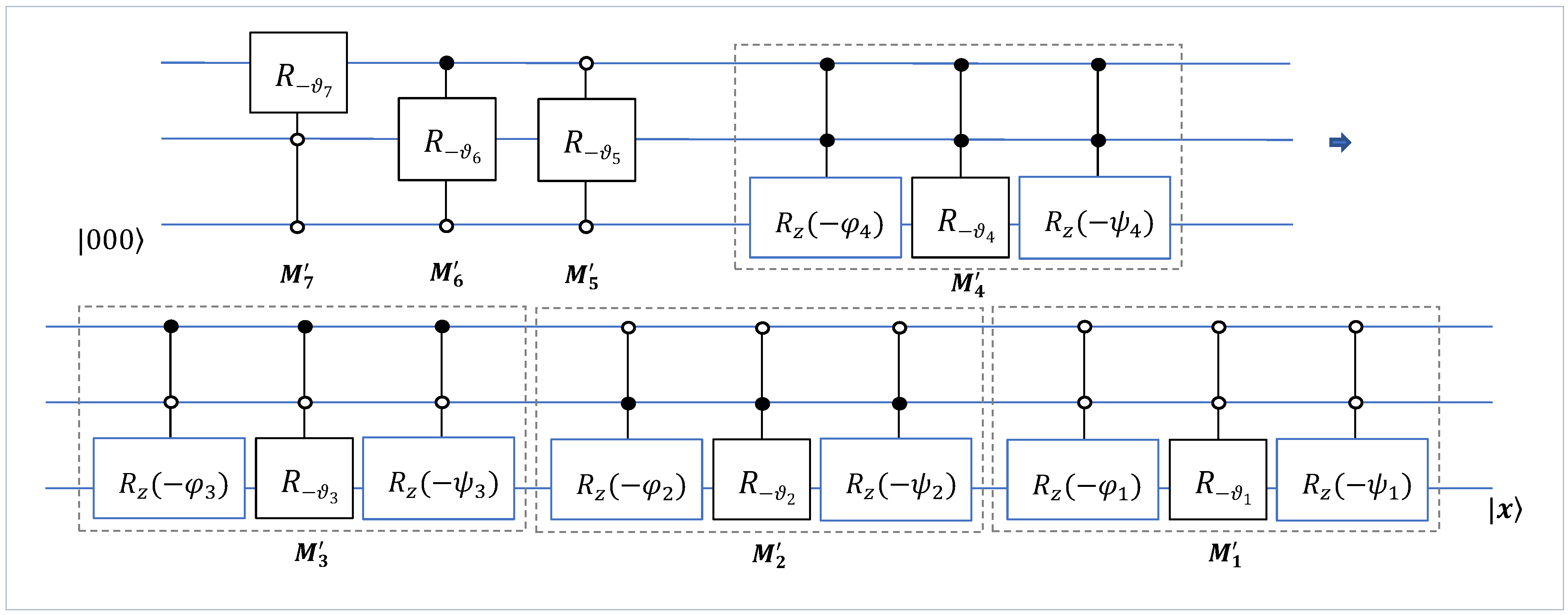
4. DsiHT-Based QR Decomposition

In this section, we describe the QR decomposition of a square unitary matrix of size $2^r\times 2^r, r>1,$ by the Givens rotations [34,38]. The unitary matrix $A=\left\{a_{i,j}\right\}$ is considered with real or complex coefficients. In this decomposition, the matrix is presented as $A=QR$, where $Q$ is a unitary matrix composed of rotations, and $R$ is a diagonal matrix with coefficients lying on the unit circle. During this decomposition, the matrix $A$ is transformed sequentially into a diagonal matrix $R$. $(2^r-1)$ DsiHTs are used in the QR decomposition of matrix $A$. The first step of this decomposition is illustrated below, for an 8 $\times 8$ unitary matrix,

$$A=\left[\begin{array}{cccccccc}{x}_0& \circ & \circ & \circ & \circ & \circ & \circ & \circ \\ x_1& \circ & \circ & \circ & \circ & \circ & \circ & \circ \\ x_2& \circ & \circ & \circ & \circ & \circ & \circ & \circ \\ x_3& \circ & \circ & \circ & \circ & \circ & \circ & \circ \\ x_4& \circ & \circ & \circ & \circ & \circ & \circ & \circ \\ x_5& \circ & \circ & \circ & \circ & \circ & \circ & \circ \\ x_6& \circ & \circ & \circ & \circ & \circ & \circ & \circ \\ x_7& \circ & \circ & \circ & \circ & \circ & \circ & \circ \end{array}\right] \stackrel{\mathit{x}-DsiHT}{\to } A_1=\left[\begin{array}{cccccccc}{x}_0^{(3)}& 0& 0& 0& 0& 0& 0& 0\\ 0& y_1& \star & \star & \star & \star & \star & \star \\ 0& y_2& \star & \star & \star & \star & \star & \star \\ 0& y_3& \star & \star & \star & \star & \star & \star \\ 0& y_4& \star & \star & \star & \star & \star & \star \\ 0& y_5& \star & \star & \star & \star & \star & \star \\ 0& y_6& \star & \star & \star & \star & \star & \star \\ 0& y_7& \star & \star & \star & \star & \star & \star \end{array}\right]\to \cdots \to R.$$

(39)

The matrix diagonalization can be described by the following steps:

1.

The first DsiHT, denoted as $H_{0-7},$ is generated by the first column $\left(a_{0,0},a_{1,0}, \dots ,a_{7,0}\right)$ of the matrix $A$, which we denote by $\mathit{x}=\left(x_0,x_1,\dots ,x_7\right).$ This transform changes this column as

$$H_{0-7}:\mathit{x}\to \left(x_0^{(3)},0,0,\dots ,0\right)=\left(\pm ‖\mathit{x}‖,0,0,\dots ,0\right).$$

(40)

After multiplying the matrix of this DsiHT by matrix $A$, the new matrix $A_1=H_{0-7}A$ will have the form shown in Equation (39). Except the first point on the diagonal, all values of the first column and row are equal to 0.

2.

The second 8-point DsiHT, denoted as $H_{1-7},$ is generated by the second column of the new matrix $A_1$, which is denoted as $\mathit{y}=\left(0,y_1,\dots ,y_7\right).$ This transform will change this column as

$$H_{8;\#2}:\mathit{y}\to \left(0,\pm ‖\mathit{y}‖,0,0,\dots ,0\right)$$

(41)

and other columns $\mathit{z}$ of the matrix $A_1$ as $H_{1-7}:\mathit{z}\to \left(0,0,z_2^{\prime },\dots ,{\mathrm{z}}_7\prime \right)$.

3.

A similar 8-point DsiHT, $H_{2-7}$, will be generated by the 3rd column of the new matrix $A_2=H_{1-7}{(H}_{0-7}A)$ and applied on it. If we denote this column as $\mathit{v}=\left(0,0,v_2,\dots ,v_7\right)$, then this transform will change this column as

$$H_{2-7}:\mathit{v}\to \left(0,0,\pm ‖\mathit{v}‖,0,0,\dots ,0\right)$$

(42)

and other columns $\mathit{z}$ of the matrix $A_2$ as $H_{2-7}:\mathit{z}\to \left(0,0,0,z_3^{\prime },\dots ,{\mathrm{z}}_7\prime \right)$.

4.

This process is continued four more times, until matrix diagonalization is completed

$$R={H_{6-7}(\dots {(H}_{2-7}(H}_{1-7}{(H}_{0-7}A)))\dots ).$$

(43)

Each of these seven 8-point DsiHTs can be defined with the fast path, as in the examples described above, which calculate these transforms only on adjacent bit planes.

In the above, for $k=0:6$, the transform $H_{k-7}$ generated by the vector $\mathit{x}=\left(x_0,x_1,\dots , x_7\right)$ does not change the first values $x_0,x_1, \dots , x_{k-1}$ of $\mathit{x}$, as well as a vector $\mathit{z}$ on which it applies. That is, it processes only the remaining components. For instance, if $k=2$,

$$H_{2-7}:\mathit{z}=\left(z_0,z_1,\underbrace{{z_2,z}_3,z_4,z_5,z_6, z_7}\right)\to \left(z_0,z_1,\underbrace{z_2^{\prime },z_3^{\prime },z_4^{\prime },z_5^{\prime },z_6^{\prime }, z_7^{\prime }}\right).$$

(44)

This 8-point DsiHT is generated under the condition,

$$H_{2-7}:\mathit{x}=\left(0,0,\underbrace{{x_2,x}_3,x_4,x_5,x_6, x_7}\right)\to \left(0,0,\underbrace{\pm ‖x‖,0,0,0,0,0}\right),$$

(45)

where $‖x‖$ is the norm of the vector, $‖x‖=\sqrt{{|x}_2{|}^2+{|x}_3{|}^2+\cdots {|x}_7{|}^2}$. Thus, the energy of the signal is moved to the third components ($k+1=3$).

These seven 8-point DsiHT with fast paths for the QR-decomposition of a matrix 8 $\times$ 8 are described in detail and with the quantum circuits in [24] for the real matrix $A$. The QR decomposition is encoded, as shown in

Table 4. The encoded table of seven QsiHTs by the fast paths in the 3-qubit QR decomposition.

QsiHT	#BPs				BFs
$H_{0-7}$	7	${\left(0,1\right)}_{\circ }^{\ast }$	${\left(2,3\right)}_{\circ }^{\ast }$	${\left(4,5\right)}_{\circ }^{\ast }$	${\left(6,7\right)}_{\circ }^{\ast }$	${\left(0,2\right)}_{\circ }^{\ast }$	${\left(4,6\right)}_{\circ }^{\ast }$	${\left(0,4\right)}_{\circ }^{\ast }$
$H_{1-7}$	6	${\left(2,3\right)}_{\ast }^{\circ }$	${\left(6,7\right)}_{\ast }^{\circ }$	${\left(1,3\right)}_{\circ }^{\ast }$	${\left(5,7\right)}_{\circ }^{\ast }$	${\left(4,5\right)}_{\ast }^{\circ }$	${\left(1,5\right)}_{\circ }^{\ast }$
$H_{2-7}$	5	${\left(2,3\right)}_{\circ }^{\ast }$	${\left(4,5\right)}_{\circ }^{\ast }$	${\left(6,7\right)}_{\circ }^{\ast }$	${\left(4,6\right)}_{\ast }^{\circ }$	${\left(2,6\right)}_{\circ }^{\ast }$
$H_{3-7}$	4	${\left(4,5\right)}_{\ast }^{\circ }$	${\left(6,7\right)}_{\ast }^{\circ }$	${\left(5,7\right)}_{\ast }^{\circ }$	${\left(3,7\right)}_{\circ }^{\ast }$
$H_{4-7}$	3	${\left(4,5\right)}_{\circ }^{\ast }$	${\left(6,7\right)}_{\circ }^{\ast }$	${\left(4,6\right)}_{\circ }^{\ast }$
$H_{5-7}$	2	${\left(6,7\right)}_{\ast }^{\circ }$	${\left(5,7\right)}_{\circ }^{\ast }$
$H_{6-7}$	1	${\left(6,7\right)}_{\circ }^{\ast }$

.

All butterflies (BF) and paths are shown in this table for all seven DsiHTs that are used in the decomposition. In other words, seven roadmaps are encoded in this table. For instance, we consider the transform $H_{2-7}$. Five butterflies are used as follows. The butterflies are numbered from left to right. The first butterfly is encoded as ${\left(2,3\right)}_{\circ }^{\ast }$, meaning that it operates on bit-planes 2 and 3, and the second output of the operation is zero (symbol ‘o’ is used). The energy of the input will be moved to the first output (symbol ‘*’ is used). This butterfly is the operation of rotation described in Equation (3). The butterfly number 4, which is encoded as ${\left(4,6\right)}_{\ast }^{\circ }$, operates on bit-planes 4 and 6 and moves the energy of the input to the second output. The first output is zero. This is the rotation described in Equation (4). The remaining butterflies of numbers 2, 3, and 5 operate on bit-planes (4,5), (6,7), and (2,6), respectively. They are operations of rotation that move the energy of the inputs to the first component, as the first butterfly. 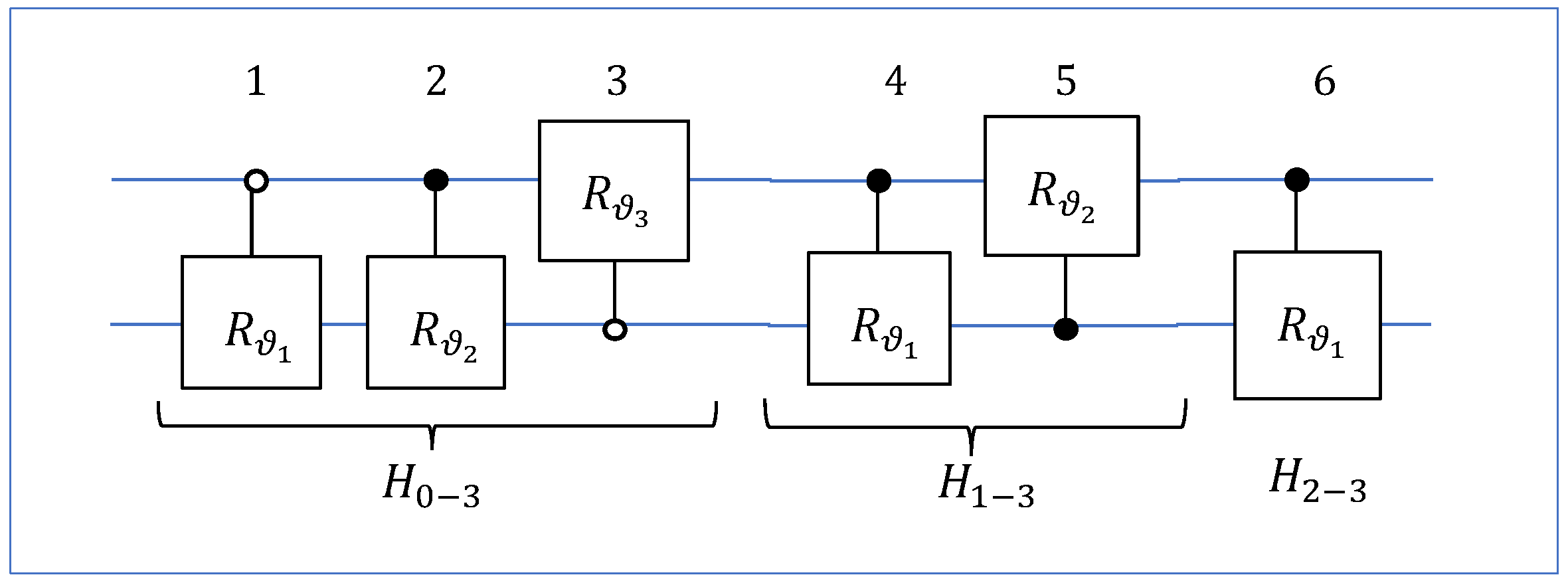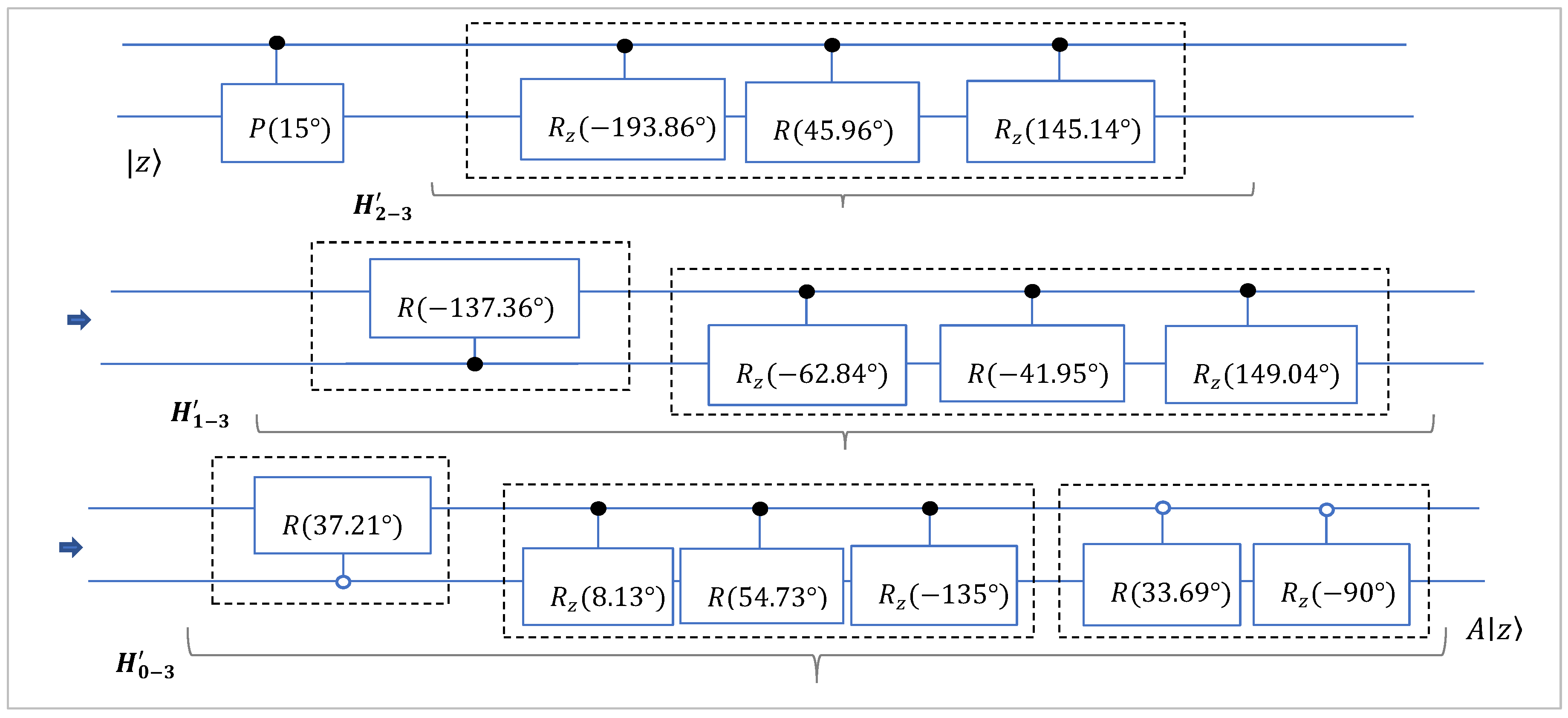The road map and the quantum circuit for the 3-qubit DsiHT, $H_{2-7}$, for the real generator are given in Figure 10.

This encoded table shows that 20 gates $M_{{\Phi }_n}$ and 8 gates $K_{{\Phi }_n}$ are used for the decomposition of the matrix. The same encoded table can be used in the case when the matrix $A$ is complex. Only the above butterflies as real gates should be changed by the corresponding complex gates $M_{{\Phi }_n}$ or $K_{{\Phi }_n}$. For instance, in the above case, the 1st butterfly ${\left(2,3\right)}_{\circ }^{\ast }$ will be changed by $M_{{\Phi }_1}$, and the firth butterfly ${\left(4,6\right)}_{\ast }^{\circ }$ should be changed to $K_{{\Phi }_4}$. The corresponding quantum circuit is given in Figure 11.

5. Two-Qubit Operations

In this section, we describe two QR-decompositions of 4 $\times$ 4 real matrix $A$ by the above method of DsiHT. First, we consider the encoded data of the decomposition, which is given in

Table 5. The encoded table for the 2-qubit QR decomposition.

QsiHT	#BPs		BFs
$H_{0-3}$	3	${\left(0,2\right)}_{\circ }^{\ast }$	${\left(1,3\right)}_{\circ }^{\ast }$	${\left(0,1\right)}_{\circ }^{\ast }$
$H_{1-3}$	2	${\left(2,3\right)}_{\ast }^{\circ }$	${\left(1,3\right)}_{\circ }^{\ast }$
$H_{2-3}$	1	${\left(2,3\right)}_{\circ }^{\ast }$

. The corresponding quantum circuit for the 2-qubit operation QR decomposition is given in Figure 12.

To simplify the notations in equation of such circuits, all rotation gates (and angles of rotations) are numbered as 1, 2, …, 7 from left to right. Therefore, the circuit in Figure 12 is described by the operation

$$H_2=R_{{\mathsf{\vartheta }}_6;2,3}\left(R_{{\mathsf{\vartheta }}_5;1,3}{R}_{{\mathsf{\vartheta }}_4;2,3}\right)\left(R_{{\mathsf{\vartheta }}_3;0,1}{R}_{{\mathsf{\vartheta }}_2;1,3}{R}_{{\mathsf{\vartheta }}_1;0,2}\right),$$

(46)

and the diagonal matrix $R=H_{2}A$.

Note that the road map for the first 4-point DsiHT, $H_{0-3}$, can be changed, as shown in

Table 6. The second encoded table for the 2-qubit QR decomposition.

QsiHT	#BPs		BFs
$H_{0-3}$	3	${\left(0,1\right)}_{\circ }^{\ast }$	${\left(2,3\right)}_{\circ }^{\ast }$	${\left(0,2\right)}_{\circ }^{\ast }$
$H_{1-3}$	2	${\left(2,3\right)}_{\ast }^{\circ }$	${\left(1,3\right)}_{\circ }^{\ast }$
$H_{2-3}$	1	${\left(2,3\right)}_{\circ }^{\ast }$

. Then, the quantum circuit for the corresponding decomposition of the 2-qubit operation will change, as shown in Figure 13,

$$H_2=R_{{\mathsf{\vartheta }}_6;2,3}\left(R_{{\mathsf{\vartheta }}_5;1,3}{R}_{{\mathsf{\vartheta }}_4;2,3}\right)\left(R_{{\mathsf{\vartheta }}_3;0,2}{R}_{{\mathsf{\vartheta }}_2;2,3}{R}_{{\mathsf{\vartheta }}_1;0,1}\right),$$

(47)

and $R=H_{2}A$. This cicuit has a depth of 5, when the circuit in Figure 12 has a depth of 4. The angles ${\vartheta }_k, k=1:7,$ and diagonal matrices $R$ for these decompositions of $A$ are different.

Next, we consider the 2-qubit complex operations and describe a quantum circuit to calculate them by using only rotation gates.

Complex 2-Qubit Operations

For 4 $\times$ 4 complex matrix $A$, the quantum circuit for the QR-decomposition by the first encoded table (Table 5) is shown in Figure 14. This circuit generalizes the circuit in Figure 12, which is given for a real matrix. There are five gates $M_{{\Phi }_k}, k=1,2,3,5,6$, and one gate $K_{{\Phi }_4}.$ The gates are numbered from left to right.

The same circuit of the decomposition operation, $H_2:A\to R$, is given in Figure 15 in a simplified form,

$$H_2=M_{{\Phi }_6;2,3}\left(M_{{\Phi }_5;1,3}{K}_{{\Phi }_4;2,3}\right)\left(M_{{\Phi }_3;0,1}{M}_{{\Phi }_2;1,3}{M}_{{\Phi }_1;0,2}\right).$$

(48)

The QR-factorization of the unitary matrix results in a diagonal matrix $R=H_{2}A$ with coefficeints lying on the unit circle. Therefore, the 3-qubit operation can be accomplished by inverting all six gates in Equation (48),

$$A=H_2^{\prime }R=\left(M_{{\Phi }_1;0,2}^{\prime }{M}_{{\Phi }_2;2,3}^{\prime }{M}_{{\Phi }_3;0,1}^{\prime }\right)\left(K_{{\Phi }_4;2,3}^{\prime }{M}_{{\Phi }_5;1,3}^{\prime }\right)M_{{\Phi }_6;2,3}^{\prime }R.$$

(49)

The inverse to the $K$ gate is calculated as $K_{\mathsf{\Phi }}^{\prime }={\left(R_z\left(-\phi \right)R\left(\gamma \right)R_z\left(-\psi \right)\right)}^{\prime }=R_z(\psi )R\left(-\gamma \right)R_z\left(\phi \right)$.

Thus, we obtain the circuit to calculate the 2-qubit operation $A.$ This circuit is shown in Figure 16 and in more detail in Figure 17.

If we use the second encoded table, namely Table 6, for 2-qubit complex operation $A$, then we obtain the circuit that is shown in Figure 18. Comparing this circuit with the one in Figure 16, one can notice the change in the part of the transform $H_{0-3}^{\prime }$. Angles are also different for all 6 complex gates.

Example 3.

Consider the following complex unitary $4\times 4$ matrix:

$$A=\left[\begin{array}{cccc}0.4685+0.4685i& 0.2810-0.5163i& -0.4049+0.1321i& 0.1224+0.1380i\\ 0.3123+0.3123i& -0.4379+0.2810i& 0.2124-0.2434i& 0.0260+0.6551i\\ 0.1562+0.3123i& -0.3987-0.0327i& -0.0777-0.5352i& 0.0391-0.6512i\\ 0.1562+0.4685i& 0.0915+0.4640i& 0.2987+0.5767i& 0.0847-0.3217i\end{array}\right]$$

(50)

with the determinant $\left|\det A\right|=1.$ All angles in the DsiHT-based QR decomposition of matrix $A=QR$ are shown in

Table 7. The angles of the rotations in the circuit of Figure 17 with encoding Table 5.

	${\mathit{\phi }}_{\mathit{k}}$	${\mathit{\vartheta }}_{\mathit{k}}$$\mathbf{\left(}{\mathit{\gamma }}_{\mathit{k}}\mathbf{\right)}$	${\mathit{\psi }}_{\mathit{k}}$	$\mathit{k}$
$H_{0-3}$	$108.4349°$	$-27.7913°$	$-18.4349°$	$1$
	$116.5651°$	$-48.1897°$	$-26.5651°$	2
	$0°$	$-41.4976°$	$0°$	3
$H_{1-3}$	$-74.9816°$	$47.8430°$	$-226.9092°$	$1$
	$54.2886°$	$-50.8961°$	$54.2886°$	2
$H_{2-3}$	$258.1788°$	$-70.1975°$	$-37.7291°$	$1$

. The encoding table is considered to be Table 5. The diagonal matrix is equal to $R=\mathrm{d}\mathrm{i}\mathrm{a}\mathrm{g}\left\{1,1,1,e^{-i\pi /12}\right\}$, which can be written with the phase gate as $R=I_2\oplus P(-\pi /12)$. The symbol $\oplus$ is used for the Kronecker sum of matrices [1]. In the last gate $M_{{\Phi }_3;0,2},$ of the tranform $H_{0-3}$, two $Z$-rotations are the identity transforms, $R_z\left(0\right)=I_2$. This gate is $Y$-rotation gate $R_{{\vartheta }_3;0,2}$.

The same diagonal matrix $R=\mathrm{d}\mathrm{i}\mathrm{a}\mathrm{g}\left\{1,1,1,e^{-i\pi /12}\right\}$ is obtained when the QR-decomposition of the matrix $A$ is calculated by encoding Table 7. In this case, the set of angles of rotations changes as shown in

Table 8. The angles of the rotations in the circuit of Figure 17 with encoding Table 6.

	${\mathit{\phi }}_{\mathit{k}}$	${\mathit{\vartheta }}_{\mathit{k}}$$\mathbf{\left(}{\mathit{\gamma }}_{\mathit{k}}\mathbf{\right)}$	${\mathit{\psi }}_{\mathit{k}}$	$\mathit{k}$
$H_{0-3}$	$90°$	$-33.6901°$	$0°$	$1$
	$135°$	$-54.7356°$	$-8.1301°$	2
	$0°$	$-37.2187°$	$0°$	3
$H_{1-3}$	$149.0489°$	$41.9525°$	$-62.8419°$	$1$
	$180°$	$-42.6315°$	$180°$	2
$H_{2-3}$	$-145.1403°$	$-45.9683°$	$193.8652°$	$1$

.

One can note that there are more angles with simple rotations than in Table 7. Therefore, we chose the quantum circuit in Figure 18 for calculating the 2-qubit operation described by the matrix in Equation (50). In the first gate $M_{{\Phi }_1;0,2}$ of the transformation ${\mathit{H}}_{0-3}$, one $Z$-rotation is the identity transform, $R_z\left(0\right)=I_2.$ Also, on the 2nd stage of the DsiHT, ${\mathit{H}}_{1-3}$, the vector-angle ${\mathsf{\Phi }}_2=\left({\phi }_2,{\vartheta }_2,{\psi }_2\right)=(180°,-42.6315°,180°)$. The following holds for the rotation gates with such angles:

$${\mathit{M}}_{{\mathit{\Phi }}_2}={\mathit{M}}_{\mathit{\pi },{\mathit{\vartheta }}_2,\mathit{\pi }}=R_z\left(\pi \right)R_y\left({\vartheta }_2\right)R_z\left(\pi \right)=R_y\left({\vartheta }_2+\pi \right).$$

(51)

This operation is described by one rotation gate $R_y$. Therefore, the circuit for the 2-qubit operation $A$ in Figure 18 can be simplified as shown in Figure 19. Here, we consider the angle ${\vartheta }_2=-42.6315°$ and 180$°-42.6315°=137.3685°.$ This quantum circuit for this operation $A$ includes six $Y$-rotations, seven $Z$-rotations, and one phase gate.

6. The Circuit for 3-Qubit Operation

The QsiHT-based QR decomposition $T:A\to R$ of a unitary matrix 8 $\times$ 8 is accomplished by seven transforms in Equation (43). Therefore, the 3-qubit operation can be calculated as

$$A=T^{-1}\left(R\right)=H_{0-7}^{\prime }{H}_{1-7}^{\prime }{H}_{2-7}^{\prime }{H}_{3-7}^{\prime }{H}_{4-7}^{\prime }{H}_{5-7}^{\prime }{H}_{6-7}^{\prime }R.$$

(52)

This operation in the case where matrix $A$ is real is described in detail in [24]. The quantum circuit uses a maximum of 28 control $Y$-rotations and one phase gate for the diagonal matrix $R$. All rotations are fulfilled on the adjacent bit planes because of the encoded Table 4. Therefore, the circuit does not use any permutation elements or CNOT gates. The same encoding table is used in the complex case of the matrix. The quantum circuit is shown in Figure 20. It uses $28\times 3=84$ rotation gates and the depth of the circuit is equal to 18 $\times$ 3 = 54. The numbers of rotation gates and depth for each 3-qubit QsiHT circuit element and its depth are in given in

Table 9. Data of the 3-qubit QsiHT-based circuit for a 3-qubit complex operation.

QsiHT	# ${\mathit{R}}_{\mathit{y}}$	# ${\mathit{R}}_{\mathit{z}}$	# Rotations	# Non-Adjacent BPs	# ${\mathit{M}}_{\mathit{\Phi }}$	# ${\mathit{K}}_{\mathit{\Phi }}$	Depth
$H_{6-7}^{\prime }$	1	2	3	0	1	0	3
$H_{5-7}^{\prime }$	2	4	6	0	1	1	6
$H_{4-7}^{\prime }$	3	6	9	0	3	0	6
$H_{3-7}^{\prime }$	4	8	12	0	1	3	9
$H_{2-7}^{\prime }$	5	10	15	0	4	1	9
$H_{1-7}^{\prime }$	6	12	18	0	3	3	12
$H_{0-7}^{\prime }$	7	14	21	0	7	0	9
Total	28	54	84	0	20	8	54

.

It is considered that the depth of each complex gate $M_{{\Phi }_i}$ and $K_{{\Phi }_i}$ is equal to 3. In the case, when the operation is real, this number is counted as 1, and the depth of the circuit is equal to $54/3=18$.

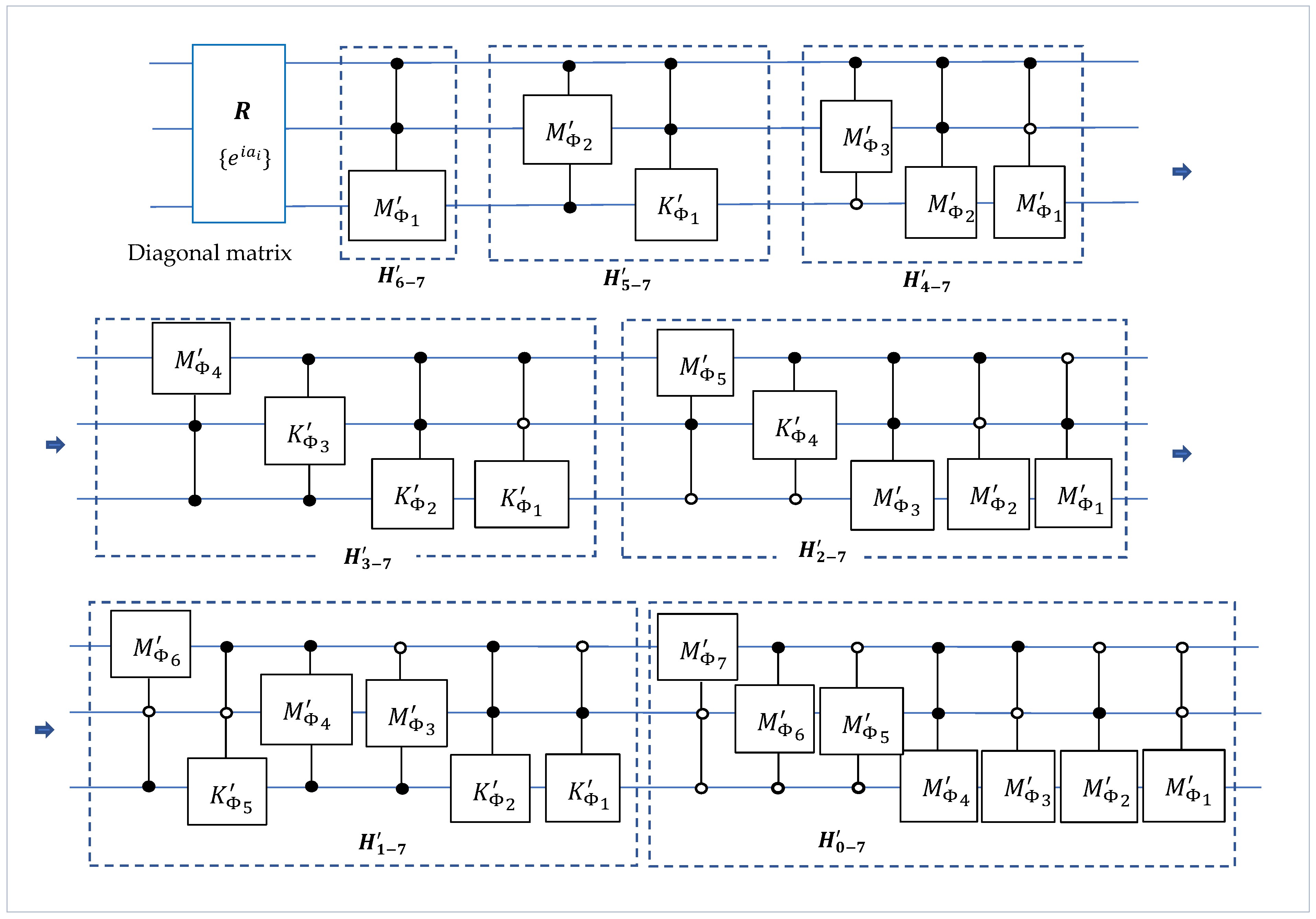
7. The Circuit for 4-Qubit Operation

In this section, we describe the circuit for calculating 4-qubit operations, which is defined by a complex unitary 16 $\times$ 16 matrix $A$. The QR-decomposition is accomplished by fifteen 16-point DsiHTs in total on 120 adjacent biplanes. The information on this decomposition

$$H_4:A\to R={H_{14-15}{(H}_{13-15}(\cdots (H_{2-15}{(H}_{1-15}(H}_{0-15}A)))))$$

(53)

is given in encoding

Table 10. The encoding table of all fifteen QsiHTs by the fast paths, which use the 4-qubit QR decomposition.

$\mathbf{Q}\mathbf{s}\mathbf{i}\mathbf{H}\mathbf{T}$	#				BPs
$H_{0-15}$	15	${\left(0,1\right)}_{\circ }^{\ast }$	${\left(2,3\right)}_{\circ }^{\ast }$	${\left(4,5\right)}_{\circ }^{\ast }$	${\left(6,7\right)}_{\circ }^{\ast }$	${\left(8,9\right)}_{\circ }^{\ast }$	${\left(10,11\right)}_{\circ }^{\ast }$	${\left(12,13\right)}_{\circ }^{\ast }$	${\left(14,15\right)}_{\circ }^{\ast }$
			${\left(0,2\right)}_{\circ }^{\ast }$	${\left(4,6\right)}_{\circ }^{\ast }$	${\left(8,10\right)}_{\circ }^{\ast }$	${\left(12,14\right)}_{\circ }^{\ast }$	${\left(0,4\right)}_{\circ }^{\ast }$	${\left(8,12\right)}_{\circ }^{\ast }$	${\left(0,8\right)}_{\circ }^{\ast }$
$H_{1-15}$	14	${\left(2,3\right)}_{\ast }^{\circ }$	${\left(6,7\right)}_{\ast }^{\circ }$	${\left(10,11\right)}_{\ast }^{\circ }$	${\left(14,15\right)}_{\ast }^{\circ }$	${\left(1,3\right)}_{\circ }^{\ast }$	${\left(5,7\right)}_{\circ }^{\ast }$	${\left(9,11\right)}_{\circ }^{\ast }$	${\left(13,15\right)}_{\circ }^{\ast }$
				${\left(4,5\right)}_{\ast }^{\circ }$	${\left(12,13\right)}_{\ast }^{\circ }$	${\left(1,5\right)}_{\circ }^{\ast }$	${\left(9,13\right)}_{\circ }^{\ast }$	${\left(8,9\right)}_{\ast }^{\circ }$	${\left(1,9\right)}_{\circ }^{\ast }$
$H_{2-15}$	13	${\left(4,5\right)}_{\circ }^{\ast }$	${\left(8,9\right)}_{\circ }^{\ast }$	${\left(10,11\right)}_{\circ }^{\ast }$	${\left(12,13\right)}_{\circ }^{\ast }$	${\left(14,15\right)}_{\circ }^{\ast }$	${\left(4,6\right)}_{\ast }^{\circ }$	${\left(12,14\right)}_{\circ }^{\ast }$	${\left(6,7\right)}_{\ast }^{\circ }$
					${\left(8,12\right)}_{\circ }^{\ast }$	${\left(3,7\right)}_{\circ }^{\ast }$	${\left(8,10\right)}_{\ast }^{\circ }$	${\left(2,3\right)}_{\circ }^{\ast }$	${\left(2,10\right)}_{\circ }^{\ast }$
$H_{3-15}$	12	${\left(4,5\right)}_{\ast }^{\circ }$	${\left(6,7\right)}_{\ast }^{\circ }$	${\left(8,9\right)}_{\ast }^{\circ }$	${\left(10,11\right)}_{\ast }^{\circ }$	${\left(12,13\right)}_{\circ }^{\ast }$	${\left(5,7\right)}_{\ast }^{\circ }$	${\left(9,11\right)}_{\ast }^{\circ }$	${\left(12,14\right)}_{\ast }^{\circ }$
						${\left(14,15\right)}_{\ast }^{\circ }$	${\left(3,7\right)}_{\circ }^{\ast }$	${\left(11,15\right)}_{\circ }^{\ast }$	${\left(3,11\right)}_{\circ }^{\ast }$
$H_{4-15}$	11	${\left(4,5\right)}_{\circ }^{\ast }$	${\left(6,7\right)}_{\circ }^{\ast }$	${\left(8,9\right)}_{\circ }^{\ast }$	${\left(10,11\right)}_{\circ }^{\ast }$	${\left(12,13\right)}_{\circ }^{\ast }$	${\left(14,15\right)}_{\circ }^{\ast }$	${\left(4,6\right)}_{\circ }^{\ast }$	${\left(8,10\right)}_{\circ }^{\ast }$
							${\left(12,14\right)}_{\circ }^{\ast }$	${\left(8,12\right)}_{\ast }^{\circ }$	${\left(4,14\right)}_{\circ }^{\ast }$
$H_{5-15}$	10	${\left(6,7\right)}_{\ast }^{\circ }$	${\left(8,9\right)}_{\circ }^{\ast }$	${\left(10,11\right)}_{\circ }^{\ast }$	${\left(14,15\right)}_{\circ }^{\ast }$	${\left(5,7\right)}_{\circ }^{\ast }$	${\left(8,10\right)}_{\circ }^{\ast }$	${\left(12,14\right)}_{\circ }^{\ast }$	${\left(8,12\right)}_{\ast }^{\circ }$
								${\left(12,13\right)}_{\circ }^{\ast }$	${\left(5,13\right)}_{\circ }^{\ast }$
$H_{6-15}$	9	${\left(6,7\right)}_{\circ }^{\ast }$	${\left(8,9\right)}_{\circ }^{\ast }$	${\left(10,11\right)}_{\circ }^{\ast }$	${\left(12,13\right)}_{\circ }^{\ast }$	${\left(14,15\right)}_{\circ }^{\ast }$	${\left(8,10\right)}_{\ast }^{\circ }$	${\left(12,14\right)}_{\ast }^{\circ }$	${\left(10,14\right)}_{\ast }^{\circ }$
									${\left(6,14\right)}_{\circ }^{\ast }$
$H_{7-15}$	8	${\left(8,9\right)}_{\ast }^{\circ }$	${\left(10,11\right)}_{\ast }^{\circ }$	${\left(12,13\right)}_{\ast }^{\circ }$	${\left(14,15\right)}_{\ast }^{\circ }$	${\left(9,11\right)}_{\ast }^{\circ }$	${\left(13,15\right)}_{\ast }^{\circ }$	${\left(11,15\right)}_{\ast }^{\circ }$	${\left(7,15\right)}_{\circ }^{\ast }$
$H_{8-15}$	7	${\left(8,9\right)}_{\circ }^{\ast }$	${\left(10,11\right)}_{\circ }^{\ast }$	${\left(12,13\right)}_{\circ }^{\ast }$	${\left(14,15\right)}_{\circ }^{\ast }$	${\left(8,10\right)}_{\circ }^{\ast }$	${\left(12,14\right)}_{\circ }^{\ast }$	${\left(8,12\right)}_{\circ }^{\ast }$
$H_{9-15}$	6	${\left(10,11\right)}_{\ast }^{\circ }$	${\left(14,15\right)}_{\ast }^{\circ }$	${\left(9,11\right)}_{\circ }^{\ast }$	${\left(13,15\right)}_{\circ }^{\ast }$	${\left(12,13\right)}_{\ast }^{\circ }$	${\left(9,13\right)}_{\circ }^{\ast }$
$H_{10-15}$	5	${\left(10,11\right)}_{\circ }^{\ast }$	${\left(12,13\right)}_{\circ }^{\ast }$	${\left(14,15\right)}_{\circ }^{\ast }$	${\left(12,14\right)}_{\ast }^{\circ }$	${\left(10,14\right)}_{\circ }^{\ast }$
$H_{11-15}$	4	${\left(12,13\right)}_{\ast }^{\circ }$	${\left(14,15\right)}_{\ast }^{\circ }$	${\left(13,15\right)}_{\ast }^{\circ }$	${\left(11,15\right)}_{\circ }^{\ast }$
$H_{12-15}$	3	${\left(12,13\right)}_{\circ }^{\ast }$	${\left(14,15\right)}_{\circ }^{\ast }$	${\left(12,14\right)}_{\circ }^{\ast }$
$H_{13-15}$	2	${\left(14,15\right)}_{\ast }^{\circ }$	${\left(13,15\right)}_{\circ }^{\ast }$
$H_{14-15}$	1	${\left(14,15\right)}_{\circ }^{\ast }$						Total #	120 BPs

.

If we use this table for a real 4-qubit operation, the QR decomposition requires only 120 rotation gates. Therefore, the quantum circuit for this operation

$$A={H_{0-15}^{\prime }{(H}_{1-15}^{\prime }(\cdots (H_{12-15}^{\prime }{(H}_{13-15}^{\prime }(H}_{14-15}^{\prime })))))R$$

(54)

requires a maximum of 120 rates $R_y$ plus one Pauli $Z$ gate for the diagonal matrix with coefficients $\{1,1,\dots ,1,1,\pm 1\}$, if the last coefficient is $-1$.

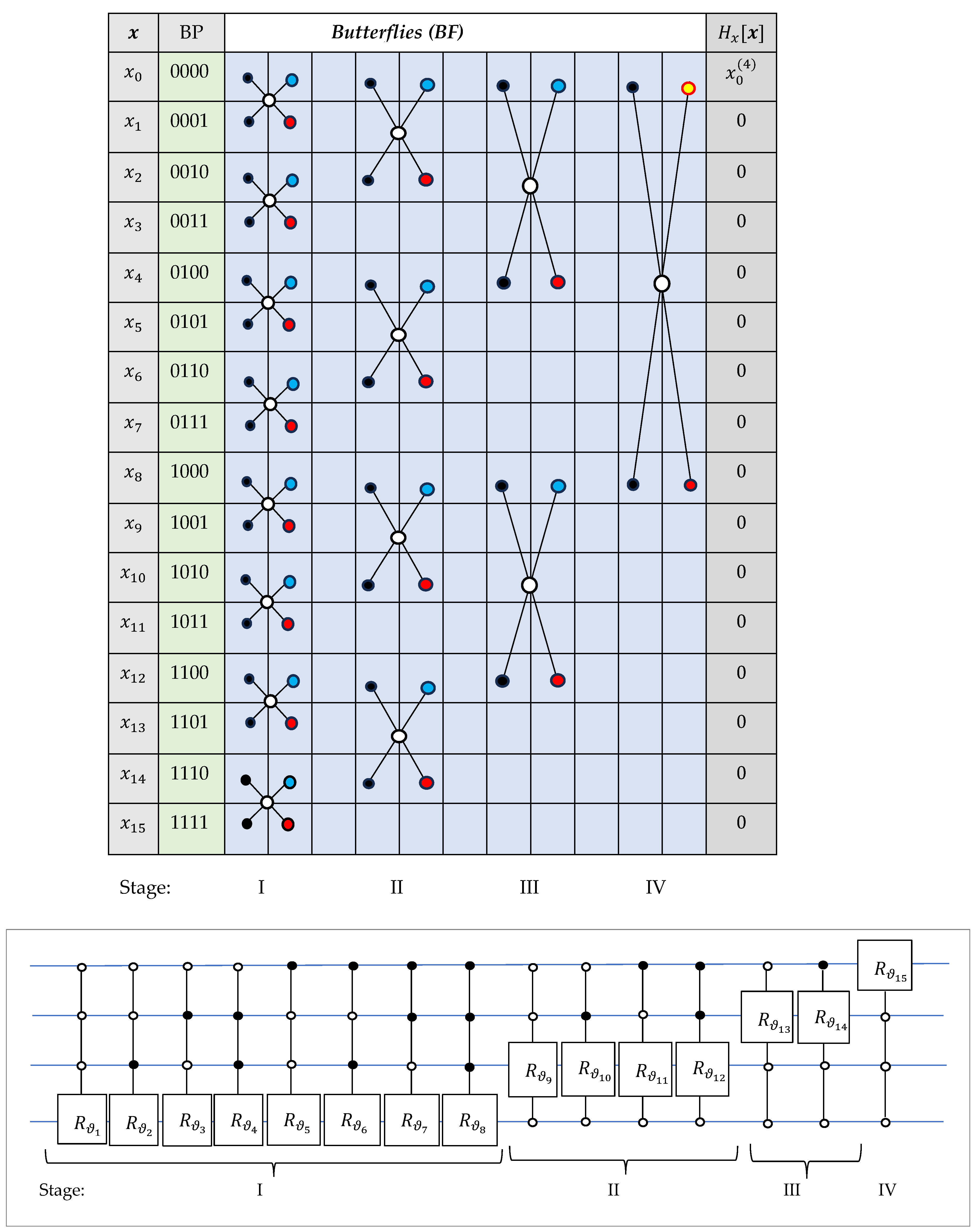
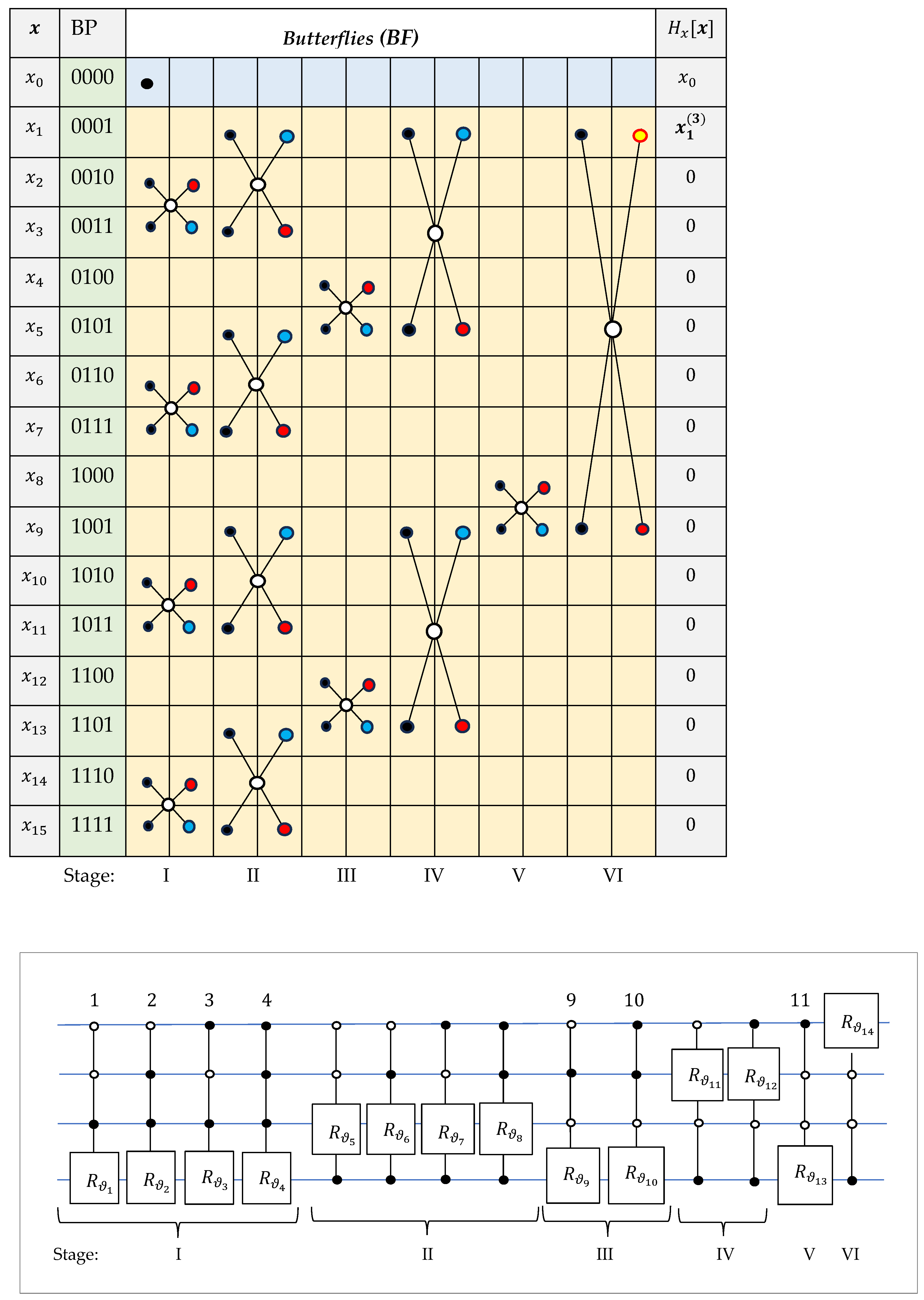
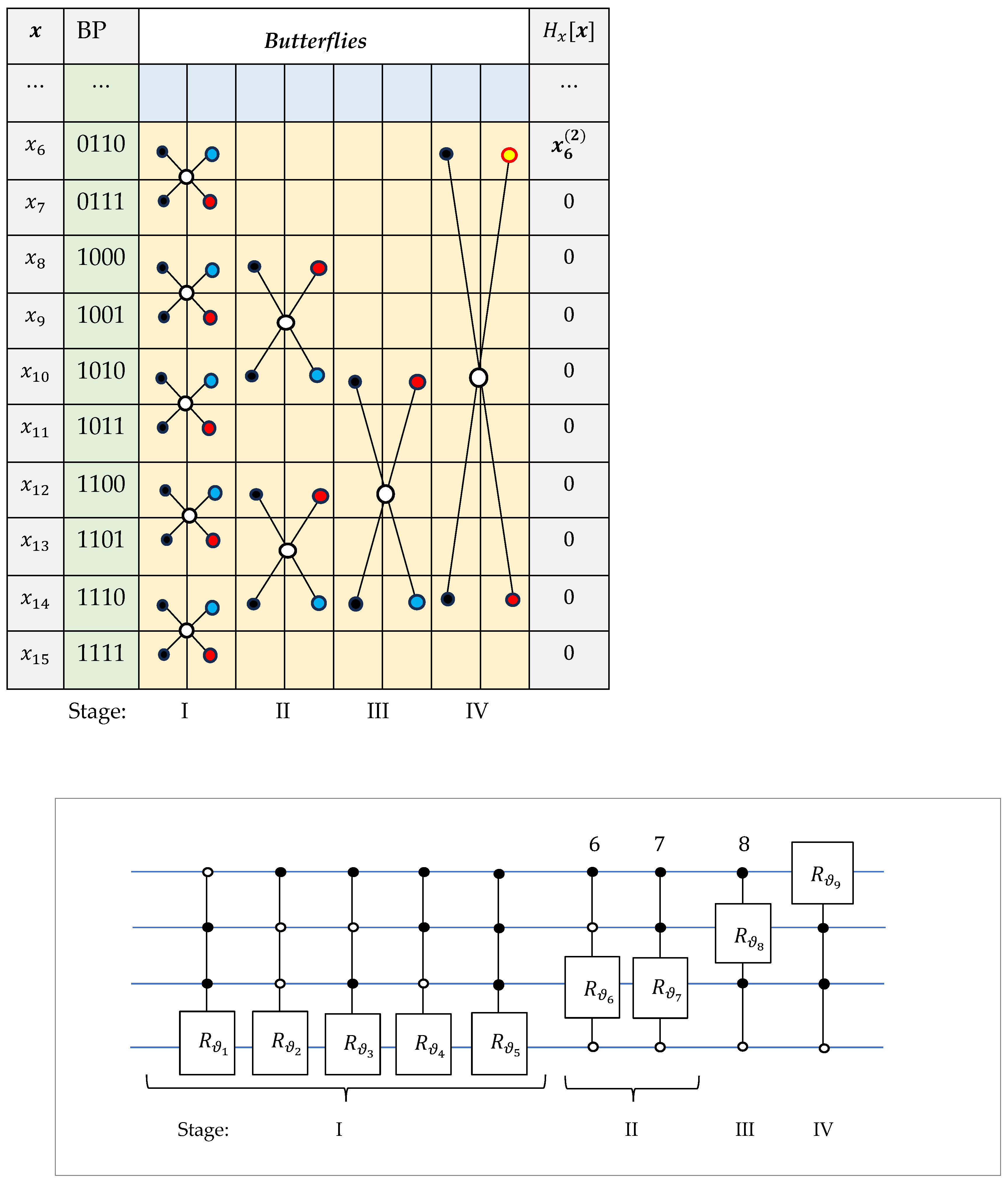
The road map for all 15 DsiHTs with fast paths are shown in Figure A1, Figure A2, Figure A3, Figure A4, Figure A5, Figure A6, Figure A7, Figure A8, Figure A9 and Figure A10 in Appendix A. The quantum circuit for these transforms are also given in these figures. As shown in Figure A9, the roadmap for the DsiHT, $H_{8-15}$, is composed of the corresponding roadmap of the 3-qubit transform $H_{0-7}$. In the circuit, we need only to add the circuit of the 3-qubit transform controlled by the first qubit. Similarly, the road maps for the last six DsiHTs, $H_{k-15}$, when $k=9:14,$ are composed of the corresponding road maps of the 3-qubit transforms $H_{(k-8)-7}$. Therefore, the quantum circuits for these transforms, $H_{k-15},$ are composed of the circuits of the transformation $H_{(k-8)-7}$ controlled by the first qubit, as shown in Figure A10.

All transforms $H_{k-15}$, when $k=0:14,$ are defined with fast paths, that is, they are composed of rotations on adjacent bit-planes only. The circuits are given for the case when the matrix of the 4-qubit operation is real. In the complex case, these rotations are substituted by the complex gates $M_{{\Phi }_i}$ or $K_{{\Phi }_i}$, as shown in the road maps. The total number of these gates is equal to 120. Among them, 40 gates are of type $K_{{\Phi }_i}.$ In all circuits, the gates are numbered from left to right. However, the numbers are shown only for $K_{{\Phi }_i}$ gates. For instance, for the transformation $H_{1-15}$, instead of rotation gate numbers 1–4, 9, 10, and 13, $K_{{\Phi }_i}$ gates are used when drawing this circuit for the complex 4-qubit operation. The remaining seven rotations will be substituted by the corresponding $M_{{\Phi }_j}$ gates.

All angles $({\phi }_j,{\vartheta }_j,{\psi }_j)$ and $({\phi }_i,{\gamma }_i,{\psi }_i)$ of these 120 complex gates represents the table of keys of the 4-qubit operation $A$. Such tables of keys are described in detail in examples for 2- and 3-qubit operation in [24]. In the general case when $n\ge 2$, an $n$-qubit operation can be decomposed by ($2^n-1$) DsiHTs with fast path. The total number of $M_{{\Phi }_i}$ and $K_{{\Phi }_i}$ gates in the decomposition is equal to $2^{n-1}(2^n-1)$. For a real $n$-qubit operation $A$, the number of rotation gates $R_y$ is equal to $2^{n-1}(2^n-1)$.

In conclusion, we consider the work of Fedoriaka [23], where the QR decomposition was implemented with Gray code and fully controlled gates. We refer to this method as the X and fully controlled gate decomposition (XFCD). The corresponding code was implemented in Q# programming language and is publicly available (for detail, see [23]). The decomposition uses $Y,Z$-rotation gates, phase gates, and X gates with matrix $X=[0,1;1,0].$ The comparison is shown in

Table 11. Comparison of circuits for two methods of QR decomposition.

Method	Gray Code	# ${\mathit{R}}_{\mathit{y}}$	# ${\mathit{R}}_{\mathit{z}}$	# Permutation/X	# ${\mathit{P}}_{\mathit{\phi }}$	# All Gates	Depth
$\mathit{n}=\mathbf{3}$
QsiHT	$-$	28	56	0	1	85	3 $\times$ 28
XFCD	$+$	28	56	28	1	113	…
$\mathit{n}=\mathbf{4}$
QsiHT	$-$	120	240	0	1	361	3 $\times$ 120
XFCD	$+$	120	240	130	1	491	…

for 3- and 4-qubit operations. We note that the XFCD was implemented for the special unitary operations, whose matrices $A$ have the determinant $\mathit{det}A=1.$ In general, for a unitary matrix $|\mathit{det}A|=1$. The proposed QsiHT-based QR decomposition method is used for any unitary operation. For special cases of $n$-qubit operations, the number of gates may be smaller, and the above quantum circuits can be reduced, or simplified, as shown in [24] with the example of Dicke states [39].

The main advantage of the proposed QR decomposition by the DsiHT with fast paths is that

• It does not require any permutations for any unitary gate in the quantum computation. It means that CNOT operations are not required.
• A maximum of ($2^n-1$) Givens rotations are gates required to perform an $n$-qubit operation with a unitary real matrix.
• A maximum of ($2^n-1$) Givens rotation and $2$($2^n-1$) $Z$-rotation gates are required to perform an $n$-qubit operation with a unitary complex matrix.
• It gives us a simple (transparent) calculation quantum circuit.
• Any $n$-qubit operation can be generated by a table of keys.
• It shows that $Y$- and $Z$-rotation plus global phase gate are a universal set of gates in quantum computation.

8. Conclusions

The QsiHT-based QR decomposition of a multi-qubit operation allows us to build quantum circuits without any permutations. All QsiHTs in the decomposition of the complex matrix use the fast paths. This is illustrated by the roadmaps given in the examples of 3- and 4-qubit operations. The corresponding quantum circuits for the matrix decomposition and calculation are described in detail. The presented method can also be generalized for quantum circuits to compute $n$-qubit operations, when $n>4$. The cases of a unitary operation with real and complex matrices are considered. For any $n$-qubit operation, a maximum of $(4^n/2-2^{n-1}$) controlled $Y$-rotation gates are only used for real operation. For complex n-qubit operation, each $Y$-rotation is combined with two $Z$-rotation gates. No permutations, including CNOTs, are used. In future works, we plan to present a universal methodology to generate any $n$-qubit QsiHT-based QR decomposition circuit beyond 4 qubits by developing automated layer-selection algorithms for the $n$-qubit QsiHT.

References

1. Nielsen, M.A.; Chuang, I.L. Quantum Computation and Quantum Information; Cambridge University Press: Cambridge, UK, 2000. [Google Scholar]
2. Rieffel, E.G.; Polak, W.H. Quantum Computing: A Gentle Introduction; The MIT Press: Cambridge, MA, USA, 2011. [Google Scholar]
3. Deutsch, D.; Barenco, A.; Ekert, A. Universality in quantum computation. Proc. R. Soc. Lond. A Math. Phys. Sci. 1995, 449, 669–677. [Google Scholar]
4. Barenco, A.; Bennett, C.H.; Cleve, R.; DiVincenzo, D.P.; Margolus, N.; Shor, P.; Sleator, T.; Smolin, J.A.; Weinfurter, H. Elementary gates for quantum computation. Phys. Rev. A 1995, 52, 3457–3467. [Google Scholar] [CrossRef] [PubMed]
5. Knill, E. Approximation by Quantum Circuits; LANL Rep. LAUR-95-2225; Los Alamos National Laboratory: Los Alamos, NM, USA, 1995. [Google Scholar]
6. Pratt, W.K. Digital Image Processing, 3rd ed.; John Wiley & Sons, Inc.: New York, NY, USA, 2001. [Google Scholar]
7. Gonzalez, R.; Woods, R. Digital Image Processing, 2nd ed.; Prentice-Hall: Upper Saddle River, NJ, USA, 2002. [Google Scholar]
8. Björck, A. Solving Linear Least Squares Problems by Gram-Schmidt Orthogonalization. BIT Numer. Math. 1967, 7, 1–21. [Google Scholar] [CrossRef]
9. Householder, A.S. Unitary Triangulation of a Nonsymmetric Matrix. J. ACM 1958, 5, 339–342. [Google Scholar] [CrossRef]
10. Rutishause, H. Simultaneous Iteration Method for Symmetric Matrices. In Handbook for Automatic Computation: Linear Algebra; Bauer, F.L., Ed.; Springer: Berlin/Heidelberg, Germany, 2017; Volume 186. [Google Scholar]
11. Golub, G.H.; Van Loan, C.F. Matrix Computations, 3rd ed.; Johns Hopkins Press: Baltimore, MD, USA, 1996. [Google Scholar]
12. Bindel, D.; Demmel, J.; Kahan, W.; Marques, O. On Computing Givens Rotations Reliably and Efficiently; LAPACK Working Note 148, UT-CS-00-449; University of Tennessee: Knoxville, TN, USA, 2001. [Google Scholar]
13. Demmel, J.; Grigori, L.; Hoemmen, M.; Langou, J. Communication-optimal parallel and sequential QR and LU factorizations. SIAM J. Sci. Comp. 2012, 34, 206–239. [Google Scholar] [CrossRef]
14. Deutsch, D. Quantum computational networks. Proc. R. Soc. Lond. A Math. Phys. Sci. 1989, 425, 73–90. [Google Scholar]
15. Vartiainen, J.J.; Möttönen, M.; Salomaa, M.M. Efficient decomposition of quantum gates. Phys. Rev. Lett. 2004, 92, 177902. [Google Scholar] [CrossRef] [PubMed]
16. Tseng, C.C.; Hwang, T.M. Quantum circuit design of 8 × 8 discrete Hartley transform. In Proceedings of the 2004 IEEE International Symposium on Circuits and Systems (ISCAS), Vancouver, BC, Canada, 23–26 May 2004; p. III-397. [Google Scholar]
17. Plesch, M.; Brukner, C. Quantum state preparation with universal gate decompositions. arXiv 2011, arXiv:1003.5760v2. [Google Scholar] [CrossRef]
18. Zhang, X.M.; Li, T.; Yuan, X. Quantum state preparation with optimal circuit depth: Implementations and applications. arXiv 2023, arXiv:2201.11495v4. [Google Scholar] [CrossRef] [PubMed]
19. Volya, D.; Mishra, P. State preparation on quantum computers via quantum steering. arXiv 2023, arXiv:2302.13518v3. [Google Scholar]
20. Pinto, D.F.; Friedrich, L.; Maziero, J. Preparing general mixed quantum states on quantum computers. arXiv 2024, arXiv:2402.04212. [Google Scholar]
21. Bergholm, V.; Vartiainen, J.J.; Möttönen, M.; Salomaa, M.M. Quantum circuits with uniformly controlled one-qubit gates. arXiv 2004. [Google Scholar] [CrossRef]
22. Mikko, M.; Vartiainen, J.J. Decompositions of general quantum gates. arXiv 2005, arXiv:quant-ph/0504100v1. [Google Scholar]
23. Fedoriaka, D. Decomposition of unitary matrix into quantum gates. arXiv 2025, arXiv:2501.07786. [Google Scholar]
24. Grigoryan, A.M.; Gomez, A.; Espinoza, I.; Agaian, S.S. Signal-Induced Heap Transform-Based QR-Decomposition and Quantum Circuit for Implementing 3-Qubit Operations. Information 2025, 16, 466. [Google Scholar] [CrossRef]
25. Yoran, N.; Short, A. Efficient classical simulation of the approximate quantum Fourier transform. Phys. Rev. A 2007, 76, 042321. [Google Scholar] [CrossRef]
26. Marquezinoa, F.L.; Portugala, R.; Sasse, F.D. Obtaining the quantum Fourier transform from the classical FFT with QR decomposition. J. Comput. Appl. Math. 2014, 235, 74–81. [Google Scholar] [CrossRef]
27. Cooley, J.W.; Tukey, J.W. An algorithm for the machine calculation of complex Fourier series. Math. Comput. 1965, 19, 297–301. [Google Scholar] [CrossRef]
28. Li, H.S.; Fan, P.; Xia, H.; Song, S.; He, X. The quantum Fourier transform based on quantum vision representation. Quantum Inf. Process. 2018, 17, 333. [Google Scholar] [CrossRef]
29. Grigoryan, A.M.; Agaian, S.S. Paired quantum Fourier transform with log2N Hadamard gates. Quantum Inf. Process. 2019, 18, 217. [Google Scholar] [CrossRef]
30. Shende, V.V.; Bullock, S.S.; Markov, I.L. Synthesis of quantum-logic circuits. IEEE Trans. Comput.-Aided Des. Integr. Circuits Syst. 2006, 25, 1000–1010. [Google Scholar] [CrossRef]
31. Möttönen, M.; Vartiainen, J.J.; Bergholm, V.; Salomaa, M.M. Quantum circuits for general multiqubit gates. Phys. Rev. Lett. 2004, 93, 130502. [Google Scholar] [CrossRef] [PubMed]
32. Shende, V.V.; Markov, I.L.; Bullock, S.S. Minimal universal two-qubit controlled-not based circuits. Phys. Rev. A At. Mol. Opt. Phys. 2004, 69, 062321–062329. [Google Scholar] [CrossRef]
33. Grigoryan, A.M. New method of Givens rotations for triangularization of square matrices. J. Adv. Linear Algebra Matrix Theory (ALAMT) 2014, 4, 65–78. [Google Scholar] [CrossRef]
34. Grigoryan, A.M. Effective methods of QR-decompositions of square complex matrices by fast discrete signal-induced heap transforms. Adv. Linear Algebra Matrix Theory (ALAMT) 2023, 12, 87–110. [Google Scholar] [CrossRef]
35. Grigoryan, A.M.; Grigoryan, M.M. Nonlinear approach of construction of fast unitary transforms. In Proceedings of the 2006 40th Annual Conference on Information Sciences and Systems, Princeton, NJ, USA, 22–24 March 2006; pp. 1073–1078. [Google Scholar] [CrossRef]
36. Grigoryan, A.M.; Agaian, S.S. Quantum Image Processing in Practice: A Mathematical Toolbox; WILEY: Hoboken, NJ, USA, 2025; p. 320. [Google Scholar]
37. Grigoryan, A.M.; Grigoryan, M.M. Brief Notes in Advanced DSP: Fourier Analysis with MATLAB; CRC Press, Taylor, and Francis Group: Boca Raton, FL, USA, 2009. [Google Scholar]
38. Cybenko, G. Reducing quantum computations to elementary unitary operations. Comput. Sci. Eng. 2001, 3, 27–32. [Google Scholar] [CrossRef]
39. Bärtschi, A.; Eidenbenz, S. Deterministic preparation of Dicke states. In Proceedings of the International Symposium on Fundamentals of Computation Theory, Copenhagen, Denmark, 12–14 August 2019. [Google Scholar]
Figure 1. Two-level DsiHT, H x , generated by (a) a signal x and applied on (b) the input signal z , and (c) the output signal.
Information 16 00621 g001
Figure 2. The road map and the circuit for the 3-qubit QsiHT.
Information 16 00621 g002
Figure 3. The second road map and the circuit for the 3-qubit QsiHT, H 8 .
Information 16 00621 g003
Figure 4. The circuit for preparing the 3-qubit state | x .
Information 16 00621 g004
Figure 5. The circuit element for 1-qubit operation M .
Information 16 00621 g005
Figure 6. The circuit element for the 1-qubit gate K .
Information 16 00621 g006
Figure 7. The 3-qubit complex QsiHT.
Information 16 00621 g007
Figure 8. The general circuit for preparing a 3-qubit state | x .
Information 16 00621 g008
Figure 9. The circuit for preparing a 3-qubit state | x in Example 2.
Information 16 00621 g009
Figure 10. The road map and circuit for the 3-qubit real QsiHT on bit-planes 2–7.
Information 16 00621 g010
Figure 11. The circuit for the 3-qubit complex QsiHT on bit-planes 2–7.
Information 16 00621 g011
Figure 12. The first circuit for the 2-qubit decomposition of the operation.
Information 16 00621 g012
Figure 13. The second circuit for the 2-qubit decomposition of the operation A .
Information 16 00621 g013
Figure 14. The quantum circuit for the decomposition of a 2-qubit complex gate A .
Information 16 00621 g014
Figure 15. The first quantum circuit for the decomposition of a 2-qubit complex operation A .
Information 16 00621 g015
Figure 16. The quantum circuit for the 2-qubit complex gate A by using the encoding Table 5.
Information 16 00621 g016
Figure 17. The quantum circuit for the operation of a 2-qubit complex gate A .
Information 16 00621 g017
Figure 18. The quantum circuit for the 2-qubit complex gate A by using the encoding Table 6.
Information 16 00621 g018
Figure 19. The quantum circuit for the operation of a 2-qubit complex operation with the matrix A in Example 3.
Information 16 00621 g019
Figure 20. The quantum circuit for the 3-qubit complex operation A .
Information 16 00621 g020