Abstract
Oscillatory neural networks have so far been successfully applied to a number of computing problems, such as associative memories, or to handle computationally hard tasks. In this paper, we show how to use oscillators to process time-dependent waveforms with minimal or no preprocessing. Since preprocessing and first-layer processing are often the most power-hungry steps in neural networks, our findings may open new doors to simple and power-efficient edge-AI devices.
1. Introduction
Oscillatory neural networks (ONNs) are analog circuits built from oscillatory building blocks. They encode information in the phase, frequency and amplitude of these oscillations and use oscillator-oscillator couplings to process data [1,2]. Given that oscillators are ubiquitous in the physical world and can be implemented with very simple circuits, ONNs have the potential to become a practical circuit technology. It is also argued that oscillatory dynamics may naturally handle computationally hard problems [3,4].
There are a number of processing tasks where ONNs were used successfully: Hopfield-network-like associative memories [5], Ising machines [4], reservoir-like devices [6], and they were even used as image classifiers with considerable success.
In many cases, ONNs do not need any training. For example, this is the case in oscillator-based Ising machines, where the problem statement itself defines the circuit parameters. If training is needed, these networks mostly use simple Hebbian learning rules to define their computing function [7]. Recently, we have shown that it is possible to use gradient-based machine learning methods directly on the circuit model of oscillators [8], which significantly extends the range of problems that such oscillator networks could solve. Also, it is possible to use equilibrium propagation [9,10,11] or other novel algorithms to create and train ONNs.
One of the main benefits of ONNs is that they offer the possibility of using very simple building blocks: oscillators are ubiquitous in the physical world or can be realized by just a few transistors (such as ring oscillators). However, the simplicity of ONN processing is undermined by the need for input pre-processing. For example, ONN-based associative memories should receive an input oscillation with a stable phase, which is not at all trivial to generate.
Pre-processing is also needed if the ONNs are to be used on time-domain data. ONN-based associative memories operate on images (i.e., on stationary patterns such as an image encoded in a phase pattern), so the time-domain data have to be first converted to an image, such as a spectrogram. This way the rich oscillatory dynamics is likely not exploited to full extent.
In this paper, we attempt to alleviate the above-mentioned problems, trying to use ONNs for the classification of time-dependent signals with minimal preprocessing. Our case studies will be on speech (vowel) recognition.
Speech recognition is one example of time-dependent processing problems. In most current algorithms it is reduced to an image processing task as most conventional neural network models are solving it by using the Mel Spectrogram of the audio signal as input to the network [12].
ONNs are dynamical systems with inherently rich dynamic behaviors. So it seems that their capabilities are not used to the full extent when only their stationary (converged) states are used in the computations. For example, if a Hopfield-type classifier is realized by an ONN, then a stationary input (an input image or pattern) is presented, and at the end, a stationary phase configuration is read out. The dynamics of the system are interesting only until it ensures convergence to a well-defined computational ground state.
When ONNs are used to process time-dependent signals, this is usually conducted in the framework of reservoir computing [13,14]. Likely, the main reason for that is that dynamical systems are difficult to train, and reservoirs do not require training of the said dynamical systems.
The novelty of our paper is that we follow a different route, attempting the design of ONNs that do not rely on reservoirs. While reservoirs have a complex, unknown internal structure, the ONN-based layers we design act as filters that extract or classify spectral features of the input signals.
In this paper, we design two types of ONN architectures, where a first layer of oscillators does the lion’s share of processing on input auditory signals. This first layer of oscillators can directly take a time-domain signal and may output a classification result or a slowly time-varying signal that may be further processed by a traditional neural network.
The first ONN architecture consists of a hidden layer, with oscillator frequencies tuned to the dominant frequency components of the incoming signals. The inputs of this ONN are the formants of the vowels to be classified. Due to the injection locking, groups of oscillators may synchronize to each other (and to the input), signaling the presence of certain components in the input. The synchronizing oscillators in the first layer may induce synchronizations in the subsequent layers, indicating the joint presence of characteristic frequency components. We show that the couplings’ strength and the frequencies of the oscillators can be optimized by machine learning methods. For certain vowel classes, we reach high (close to 100 %) classification accuracy with the oscillators alone.
The second ONN we demonstrate is a single-layer ONN, which needs no preprocessing at all: instead of receiving formant frequencies, this ONN receives vowel waveforms directly and groups of oscillators respond directly to such stimuli. This ONN needs additional layer(s) of traditional neural networks for a high accuracy output, but we will demonstrate that the “heavy lifting” is still conducted by the ONN layer.
Both architectures belong to frequency-based ONNs, where the input and output of the computation are encoded in frequencies instead of phases [15,16]. These types of oscillators arise in various oscillator-based computing fields, such as computational neuroscience [17] and mathematical oscillators, such as modified Kuramoto-oscillators [18].
It is important to emphasize that the goal of our work is not to further the state-of-the-art in neural network accuracy or to compete with large-scale models containing millions of parameters. Instead, our aim is to demonstrate that oscillator-based systems can serve as simple, energy-efficient front-end layers in neural networks. Such systems have the potential to reduce or even eliminate the need for components like analog-to-digital (A/D) converters and spectrum analyzers.
Our work paves the way for direct processing of dynamic, time-domain signals. This likely results in significant energy savings; as in a typical edge-AI architecture, the first layer is the one that should process raw data and also this layer is responsible for the majority of the task at hand; energy savings in these layers could be the most impactful.
2. Materials and Methods
2.1. Simulation of Coupled Ring Oscillators
Ring oscillators are one of the simplest oscillators. They are built from an odd number of inverters connected in a ring shape [8]. They are easy to implement, but they possess inherent nonlinearities that make them suitable for complex, dynamic computing tasks.
Ring-oscillators can be coupled together by one of their nodes, and depending on which nodes are coupled together, there can be either a positively or a negatively coupled oscillator pair [19]. The former means that the oscillators would try to align in phase and the latter means the opposite, so they will try to align in an anti-phase state. In both cases, their frequency will pull toward each other. Since we are interested in a frequency-based ONN (i.e., phases are not directly relevant), we only use positive couplings.
In our computational study, we use a differential-equation-based (ODE-based) model of ring oscillators, following the formalism of [8]. This should give results very closely matching a behavioral SPICE simulation model.
Several oscillators coupled together can be described mathematically by the following ODE as presented in [8].
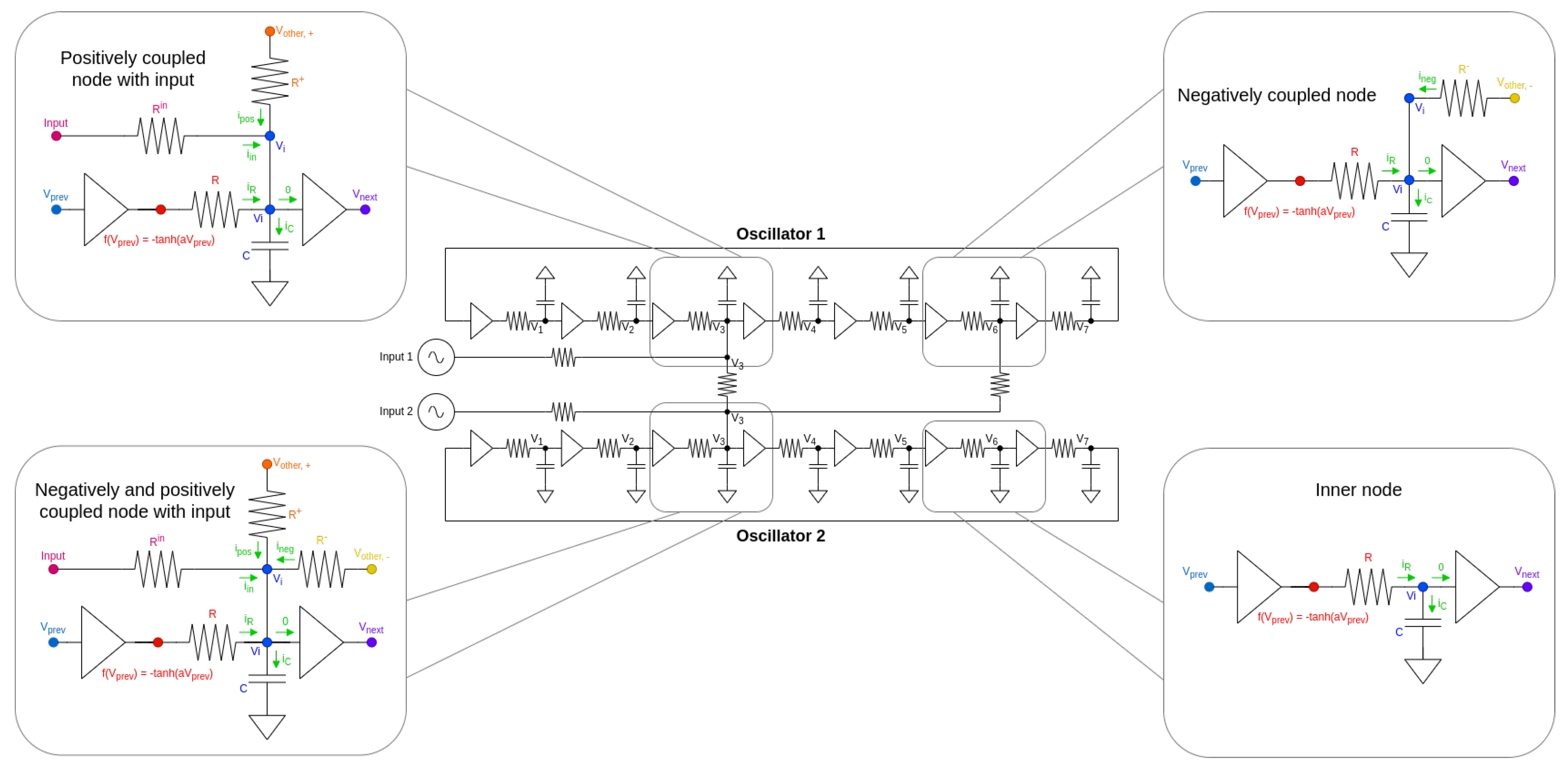
This ODE is derived using Kirchoff’s law and, for specific parts, see Figure 1. The in the equation is a permutation matrix to set the voltages according to the ring structure. is a diagonal matrix and is used to set the frequency of the oscillators by modifying the resistance between the inverters in a given oscillator. and are coupling matrices used for couplings between the oscillators and between the input generators (denoted by u) and oscillators. The function describes inverter nonlinearity. In this particular equation the input generators are considered to be voltage generators but current generators can also be used with a slightly modified ODE.
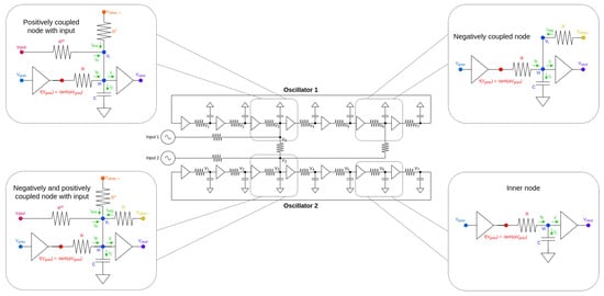
Figure 1.
The architecture of a two-oscillator system. The oscillators are coupled both positively (node 3-3 connection) and negatively (node 6-3 connection). Also, the different types of nodes in terms of connectivity that can occur in a ring oscillator are highlighted on the sides. For generality, the figure shows both positive (in-phase) and negative (anti-phase) couplings, but we only used positively coupled oscillators in this work.
Any kind of ring-oscillator-based architectures can be designed by figuring out the , and matrices. In physics, this translates to setting the values of resistances appropriately. This can be conducted by either a machine learning method based on some learning criteria or for a smaller system, these can also be set by a trial-and-error method “by hand”.
2.2. Frequency-Based Computing
Our frequency-based computing scheme is based on the simple fact that two oscillators that are synchronized to a common driving signal, become synchronized to each other as well, a phenomenon well known in the mathematial literature of synchronization [5,20]. So, certain frequency components in the driving signal can be detected by detecting the mutual synchronization of otherwise independent oscillators.
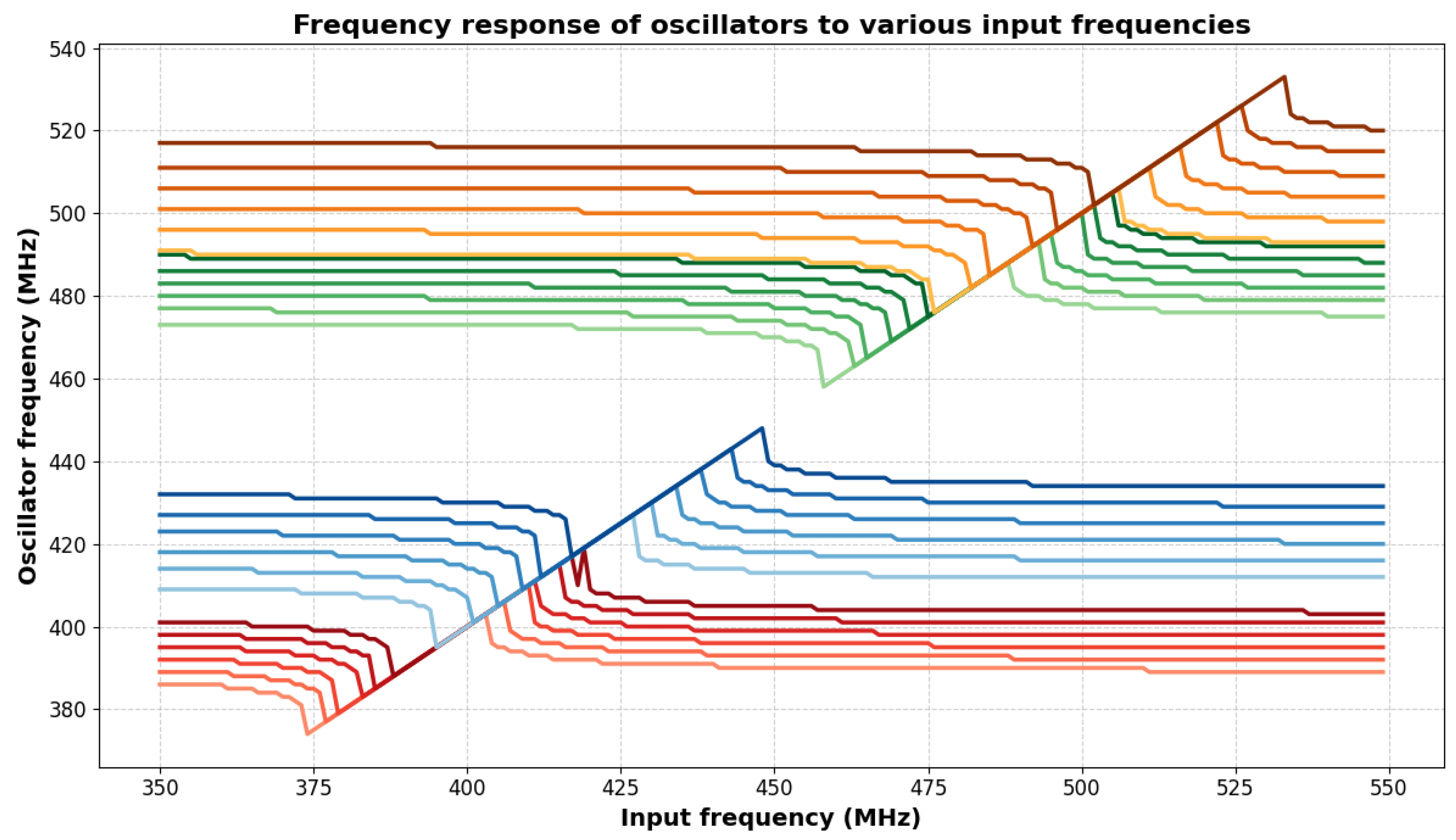
It can be observed that if a sinusoid signal arrives to one of the nodes of an oscillator, then the oscillator is capable of synchronizing its frequency to the frequency of the input signal, given that the frequency of said input signal is sufficiently close to the principal frequency of the oscillator to which it is connected. This interaction with several oscillators can be seen on Figure 2. The oscillator frequencies are grouped in the image, so it contains four groups of six oscillators having frequencies close to each other inside the groups, but relatively far away from each other between the groups. The frequency of an input sinusoidal voltage generator is swept with a frequency shown on the x axis. It can be seen that when the frequency gets close to the frequency of a group of oscillators, all the oscillators in that specific group jump together ( synchronize) in frequency.
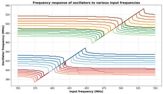
Figure 2.
Frequency synchronization of oscillators to input sinusoid with certain frequencies. A frequency sweep over a range of frequencies for a single input sinusoid voltage generator connected to a 24-uncoupled oscillator network can be seen. The four different groups of oscillators are either synchronizing to the input signal or not synchronizing to it, depending on the frequency of the input. In each group, the oscillators synchronize to the input signal’s frequency one-by-one, until all of them are synchronized, then they run together for a specific frequency range, and then they depart in frequency from the rest of the group one-by-one again.
2.3. Vowel Database and Preprocessing
To test our ONN system, we used a relatively simple, well-tested set of English spoken vowels, as described in [21].
The database we used is comprised of 12 vowels: “ae”, “ah”, “aw”, “eh”, “ei”, “er”, “ih”, “iy”, “oa”, “oo”, “uh”, “uw”. Also, the dataset we used had signals of maximum 1 s long spoken vowels with 16,000 Hz as sampling frequency. First, we padded all the vowels with zeros to have exactly 1 s length. There are recordings by both men and women in the dataset.
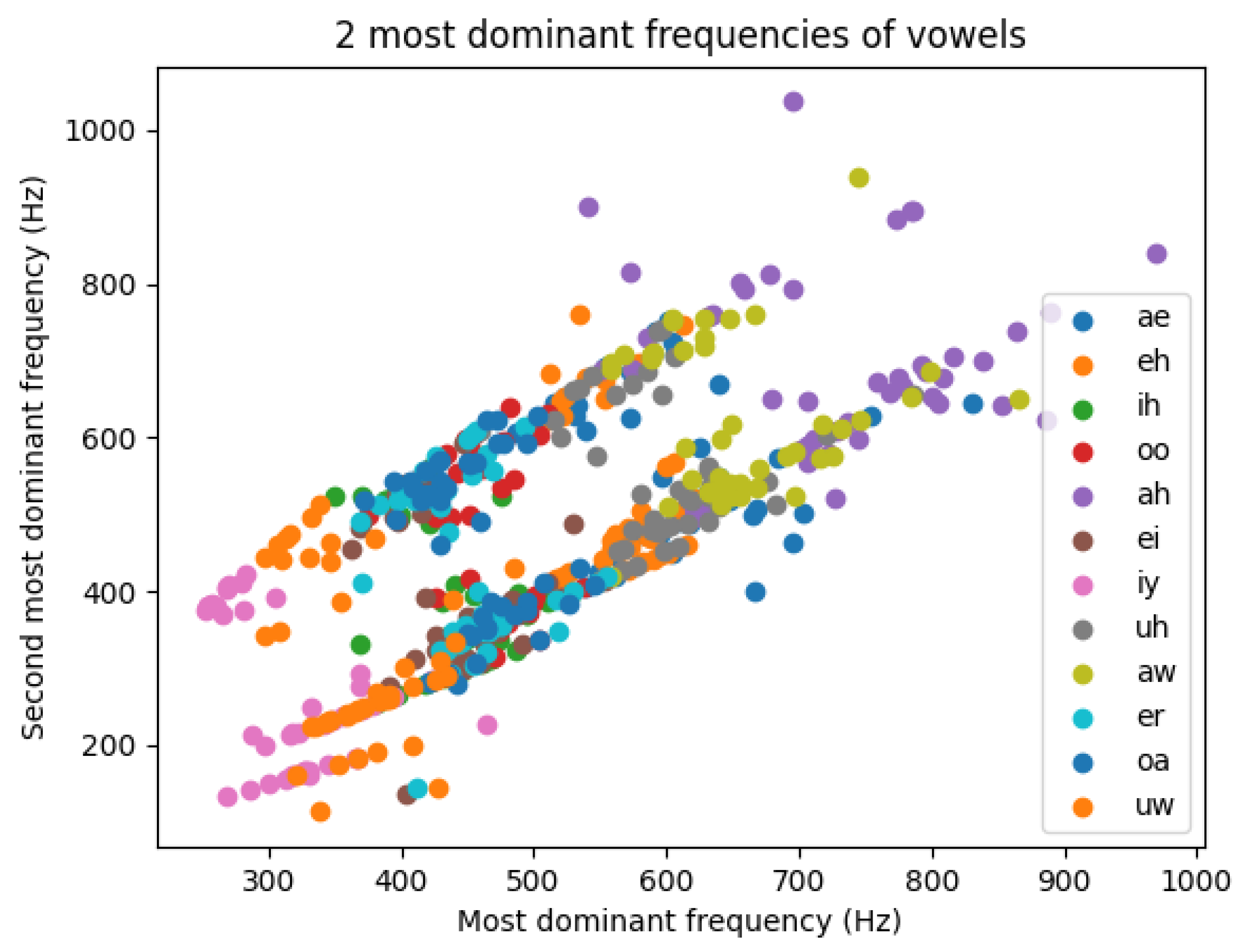
These vowels have two to four dominant frequency components, but in most cases, their two most dominant frequency components are significant enough to extract them and use them as preprocessed, synthetic sinusoidal signals as inputs to an oscillator-based architecture. The scatter plot of all the vowels’ first two formants can be seen in Figure 3. The two distinct regions where the data points are scattered—the two parallel lines—are coming from the gender differences between the speakers.

Figure 3.
Scatterplot of all the first and second most dominant frequencies of all the vowels in the dataset. The two different lines the data points are gathered around are possibly arising from the fact that these vowels were recorded by either male or female speakers and female speakers tend to have a higher pitch.
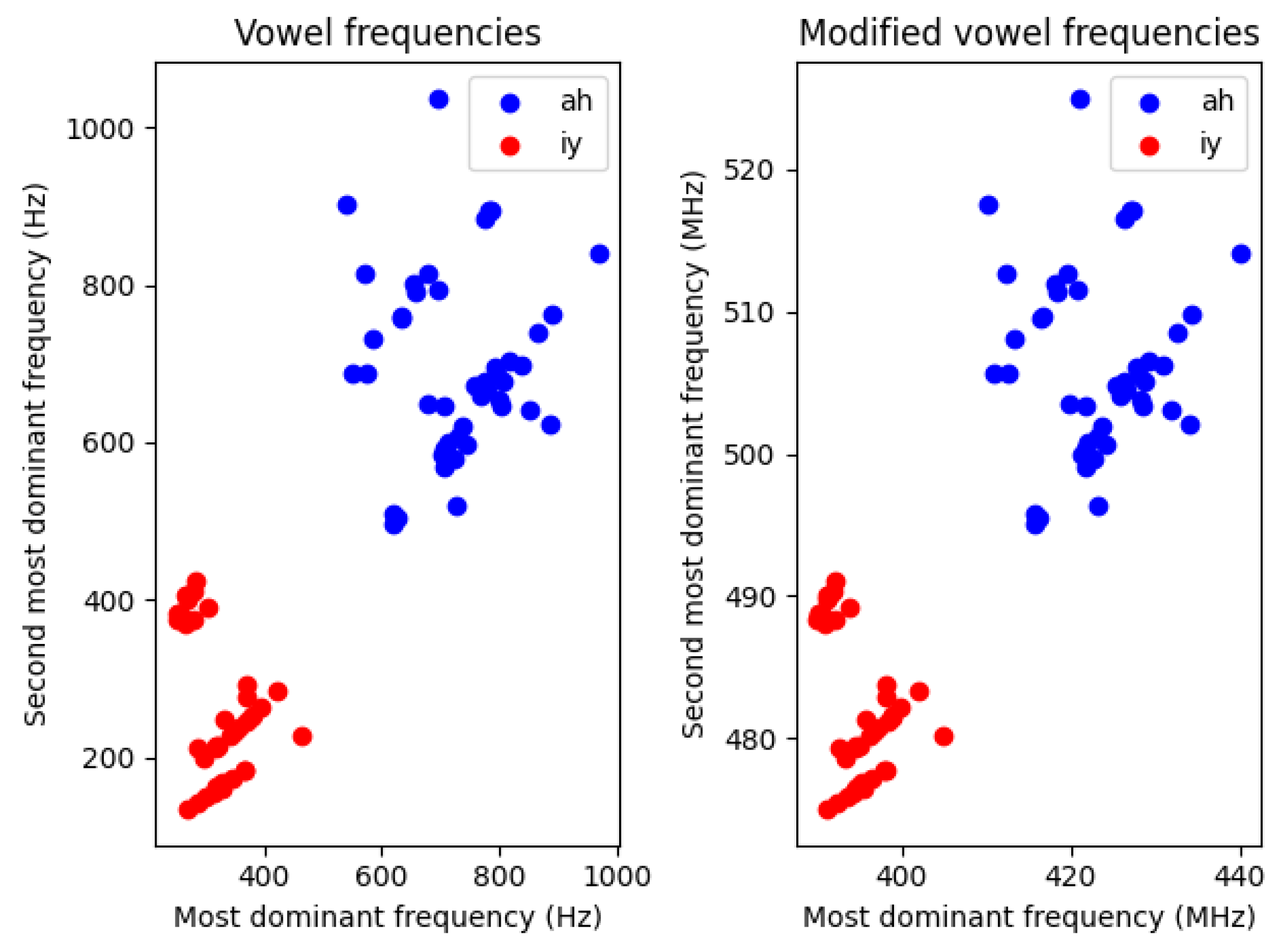
For our simulations, we utilized both the raw waveforms and the formants extracted from them. In each case, the time axis was scaled so that vowel frequencies, originally in the 100–1100 Hz range, were shifted to the 100–1100 MHz range. This scaling was necessary to ensure realistic parameters for the oscillator network, bringing its frequencies into the high MHz to low GHz range.
2.4. Vowel Recognition by Frequency-Based Computing
The key to the operation of our scheme is that oscillator groups detect frequency components in the input waveform. This phenomena can be used to detect audio signals comprised of a few amount of dominant frequency components, like English vowels.
A key requirement for the operation of this scheme is the proper choice of oscillator frequencies, which match typical vowel frequencies. The frequencies are learnable parameters that can be determined either by gradient-based or gradient-free optimization techniques.
2.5. Optimization of Parameters
Optimizing the ONN networks means finding the right parameters in the , and matrices from Equation (1). In the simplest case, this can be done by a trial-and-error method, for example, frequencies can be estimated from Figure 3. Other methods can also be used, like Backpropagation Through Time (or BPTT) [22], or gradient-free optimization. We decided to use the first trial-and-error and third gradient-free optimization approaches as we showed earlier that BPTT for ONNs consumes a lot of memory and it takes a lot of time to use [8]. As opposed to this, gradient-free optimization can be a great way to free ourselves from the burden of a method with a heavy computational cost.
Gradient-Free Optimization
Gradient-free optimization is often used when calculating the derivative of some kind of loss function is costly or even impossible. The base idea is the same as it is for the gradient-based methods, so the goal is to optimize some kind of cost or loss function. There are a lot of variations for this kind of optimization, such as evolutionary algorithms. In order to utilize gradient-free optimization, we used the Nevergrad Python package [23]. We use this method for finding the right natural (free-running) frequencies of the oscillators.
2.6. Time-Domain Vowel’s Effect on Oscillators
In the scenario of Figure 2, the oscillators are subjected to a coherent, sinusoidal injection signal. Waveforms to be classified are typically a far cry from this: most time series are wideband signals with continuously and abruptly shifting frequencies, and typically, many different frequencies are acting simultaneously on a particular oscillator.
In the circuit model, an arbitrary waveform (such as a vowel waveform) can be straightforwardly applied to the oscillators. We have conducted this by connecting an additional voltage generator through a resistor to a ring oscillator node.
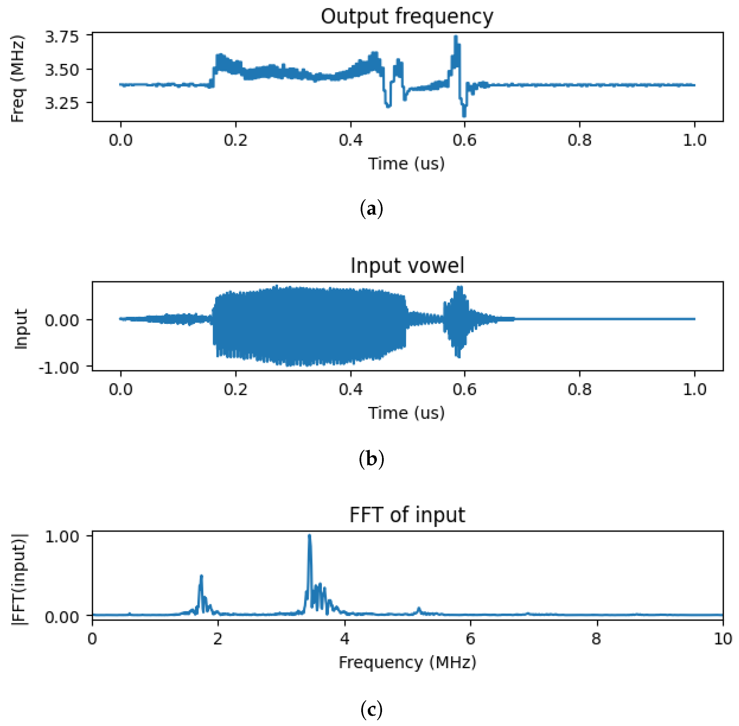
The effect of a vowel waveform on an oscillator is exemplified in Figure 4. The actual waveform is given in Figure 4b and its Fourier spectra is in Figure 4c. As described above, the sampling frequency was scaled to fall close to the natural frequency of the oscillator.

Figure 4.
(a) The effect of a time-domain waveform on a single oscillator’s frequency. (b) depicts a single vowel in time-domain. (c) shows the frequency domain of the vowel. It is evident that the most dominant frequency components of this particular vowel is around 3.50 MHz. Note that this vowel has been increased in speed, hence in frequency, by applying it over 100 s instead of 1s. On (a), the frequency response of a single oscillator can be seen, through which the input vowel has been fed by a voltage generator. It is evident that the oscillator’s frequency is changed when the input vowel is spoken on the recording and synchronized to around 350 MHz, and then it goes back up to its intrinsic frequency of around 330 MHz. This shows that ring oscillators are capable of reacting to external stimuli with their frequency, even if the input is not coherent.
In Figure 4a the instantaneous frequency of the oscillator is shown, this was simply determined from the time period of the oscillation. The time-dependent waveform is continuously pulled to the dominant frequency of the waveform as long as the vowel waveform is acting on the oscillator.
It is evident that when the vowel is actually spoken in the recording, the frequency of the oscillator is changed and synchronized to the principal frequency of the input vowel for the time being, and when the speaker stops saying the vowel, it goes back to the natural frequency of the oscillator.
Clearly, the effect of the oscillator may be viewed as a ’filter’—its frequency is pulled when a close-by frequency component appears in the input. Importantly, this effect survives even in the case of the highly incoherent input.
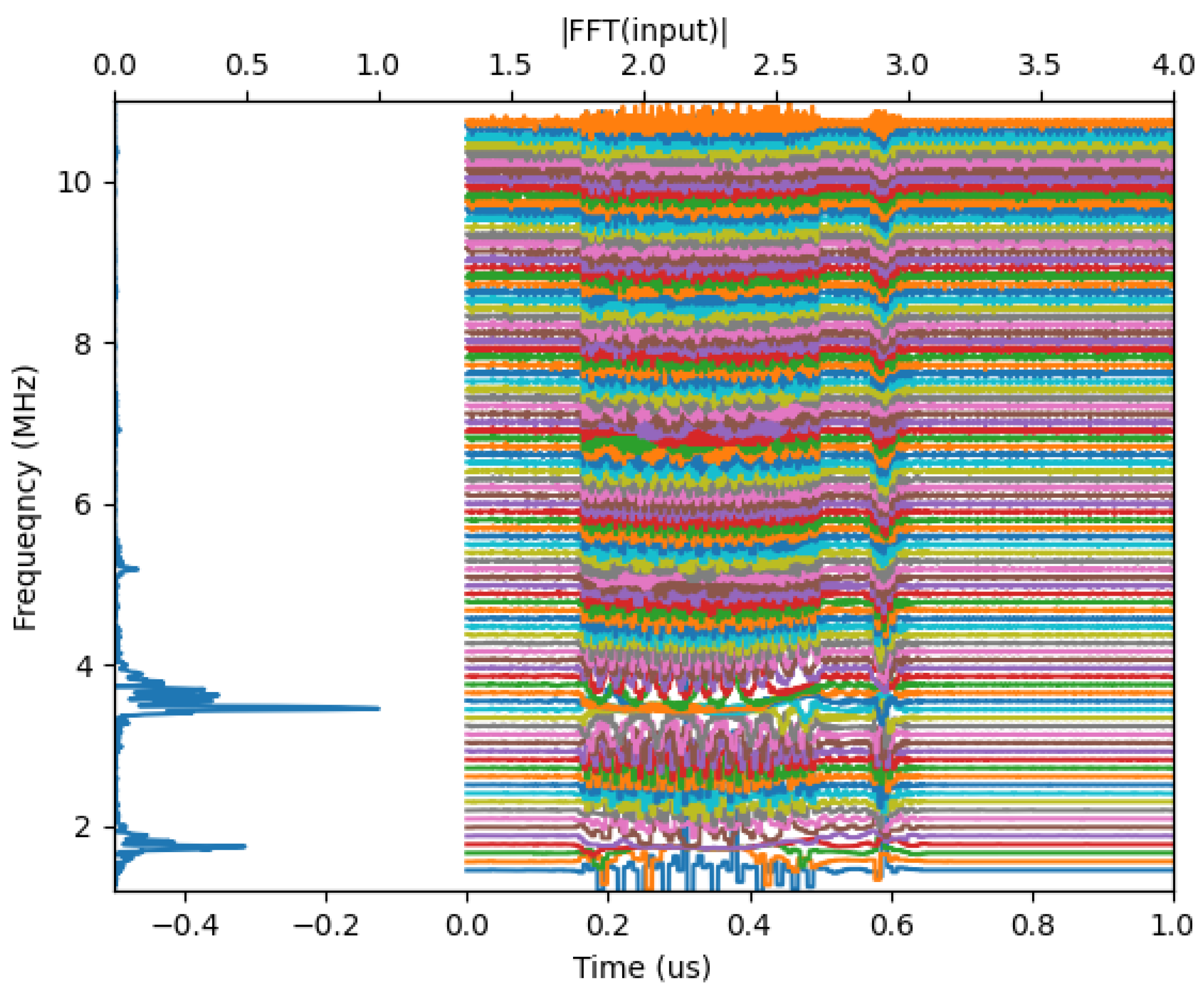
To use this effect for vowel recognition, we apply the oscillator waveforms simultaneously to a number of oscillators, whose frequencies span the range of frequencies in the vowel. The behavior of an oscillator filter bank for one particular input is shown in Figure 5, where again the instantaneous frequencies are plotted as a function of time. One can see that groups of oscillators (with closely lying frequencies) jump together when the vowel waveform is acting. Oscillators with farther-away frequencies are affected by the vowel, but they do not sync in frequency. It is important to note that oscillators that frequency-synchronize in this scenario are typically not phase-synchronized, and their waveforms do not overlap.

Figure 5.
Layer of oscillators frequency response to a single, time-domain input vowel. The oscillators with intrinsic frequencies close to the frequency peaks are synchronized in frequency to each other for the time the vowel is actually spoken and then return back to their original frequencies. Colors are used only for better visibility.
Qualitatively, the oscillator layer may be looked at as a filter bank, where the presence of a particular frequency component is signaled by the synchronization of oscillators around that frequency.
2.7. Integrating the ONN Layer with Traditional Neural Networks
For some of the results below, we used the ONN in tandem with traditional layers; these were used to improve the results coming from the oscillator layers.
For the training of this conventional, multi-layered perceptron introduced in the next section, we used standard training methods, such as Adam optimizer and cross-entropy loss. These were implemented in Pytorch [24]. Due to the small nature of this added network, the learning itself was fast and lightweight.
3. Results
In this section, we introduce two architectures for vowel classification.
The first architecture is a two-layer neural network entirely made of oscillators. This one uses two of the extracted dominant frequencies (formants) of the spoken vowels as inputs.
The second architecture uses ONN as a first layer, and classification is conducted in the second, conventional (perceptron-type) layer. This structure takes the vowel waveforms directly as inputs, with no preprocessing.
Both architectures are tested on a binary classification problem to prove that they are capable of solving tasks accurately.
For both architectures, we created a binary recognition problem to test their performance. We picked the “ah” and “iy” vowels as our test case.
3.1. Vowel Recognition by Multi-Layered Oscillatory Neural Network
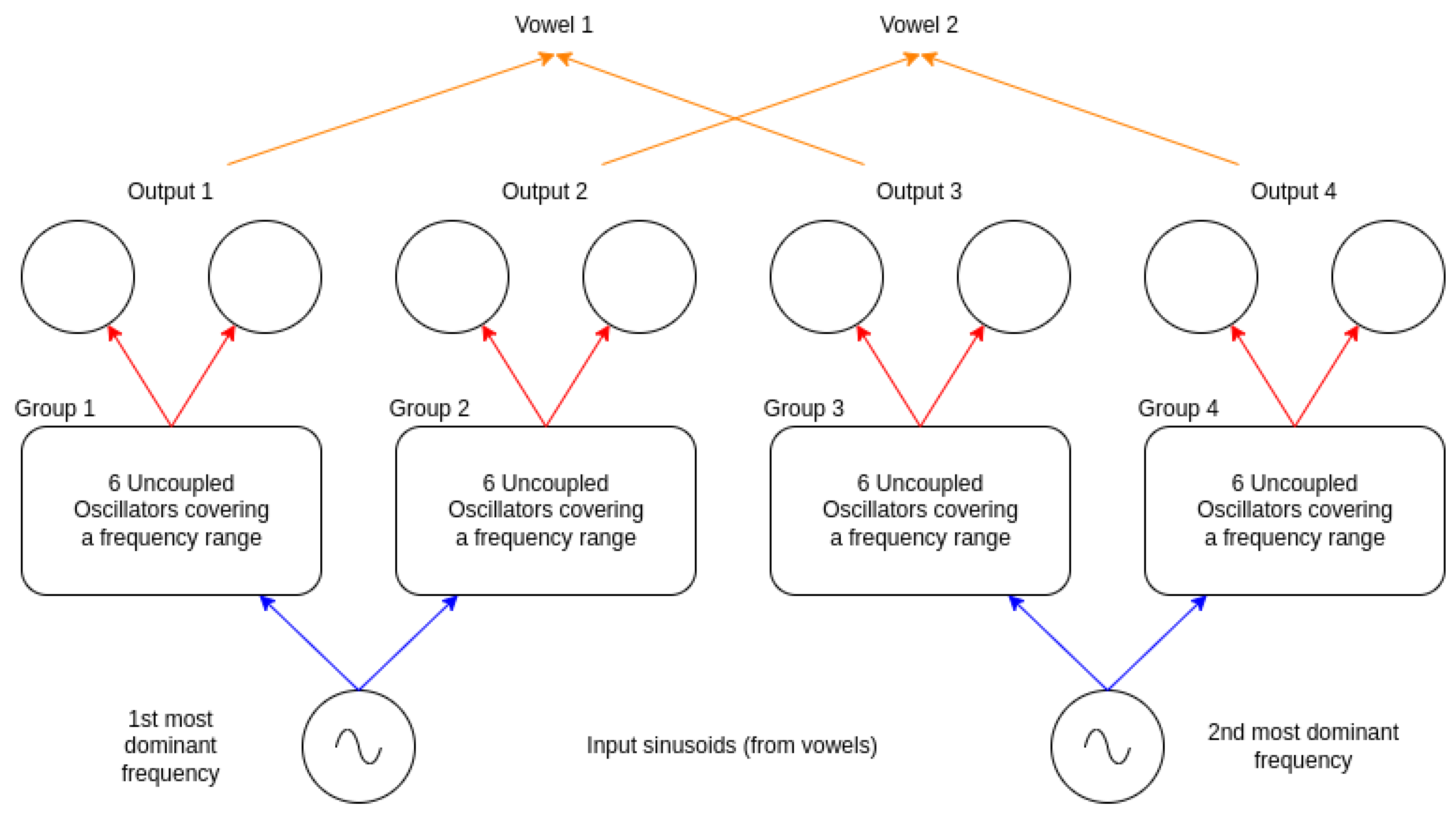
The first architecture we propose to distinguish two vowels from each other based on their two most dominant frequency components is composed of two layers and can be seen in Figure 6.
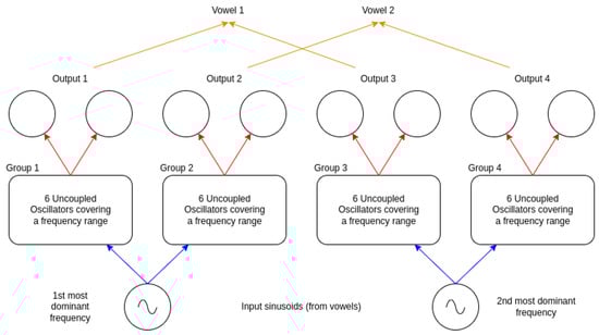
Figure 6.
Our proposed architecture. The input signals are represented as sinusoid voltage generators. The frequency of these generators is set by the first and second most dominant frequency components of a given input vowel. These are connected to a single layer of unconnected oscillators grouped into 4 distinct groups to highlight their collective responsibility in detecting a certain frequency value from the input signal. The groups are synchronized in frequency if the input sinusoid has a frequency within the frequency range the group is covering. These groups are then connected to a pair of oscillators covering the same frequency range. If the 6 oscillators in either group are synchronized in frequency, then the pair of oscillators in the output layer will be synchronized in frequency as well. This way, we can signal certain frequencies by different groups found in the input sinusoids.
The two oscillator layers do not have any intra-layer couplings, so no oscillator in a given layer is connected to any other oscillator from the same layer.
The two layers serve two distinct purposes. The first layer detects the frequency components from the input signal, and the frequency synchronization of the two oscillators shows the location of a certain frequency in the input. The second layer performs the actual classification step by detecting the pair of formants that are characteristic of the vowel.
First, the two frequency values are turned into two distinct sinusoidal signals with the given frequencies. These two signals are then fed to each of the oscillators in the first layer.
The oscillator groups in the first layer of Figure 6 are used for detecting the presence of frequency components. Due to the fact that we used the two frequency components and did binary recognition with the architecture, there are four possible different frequency combinations. The first layer’s task is to signal whether these four frequency ranges are present in the input sinusoids or not.
This frequency detection is then fed forward to the second layer. Each of the four groups in the first layer is connected to two oscillators from the output layer. The mechanism in the second layer is simple: if the oscillators in the group from the first layer are synchronized in frequency, then the two oscillators from the second layer that they are connected to will also synchronize in frequency. This way, with a simple frequency measurement in the second layer, it is possible to determine which frequency ranges were present in the input sinusoids.
This is a very simple architecture with a low number of connections. The number of couplings and oscillators is summarized in Table 1.

Table 1.
Table of neuron, coupling and parameter counts for the proposed, multilayer oscillatory network. The network is lightweight with only 50 couplings. Note that the real parameter count for the network to figure out is the sum of the number of parameters and couplings as the former is responsible for setting the frequency of oscillators and the latter is responsible for setting the strength of couplings between each connected oscillators.
To test the performance of the network, we extracted the dominant frequencies of the previously mentioned vowels. The scatter plot of these data points can be seen in Figure 7. Both the baseline frequencies and the scaled frequencies are in the figure.

Figure 7.
The dataset, consisting of two vowels “ah” and “iy” we used to test the proposed architecture. This is a linearly separable problem, so the architecture should have no difficulty solving it.
It is worthwhile to note that this network is expected to correctly classify only linearly separable problems, which is the case for the vowels shown in Figure 7 above.
3.1.1. Choosing the Network Parameters for High-Accuracy Classification
In order to optimize the network of Figure 6, the frequency of oscillators and the coupling strength between the input voltage generators and the hidden layer, and also between the hidden and the output layers, have to be set. The coupling strength translates physically to resistance values. In this section, we are showing the results of doing this by simple considerations.
Since the problem involves four distinct frequency ranges—where vowels can be differentiated based on their primary and secondary dominant frequencies—configuring the frequencies for the hidden and output layers is somewhat easier. We only needed to determine the frequencies of the grouped oscillators that could interact with the input sinusoids. Additionally, we had to select a coupling strength between the oscillators that would avoid distorting the signals and prevent overlapping synchronization regions.
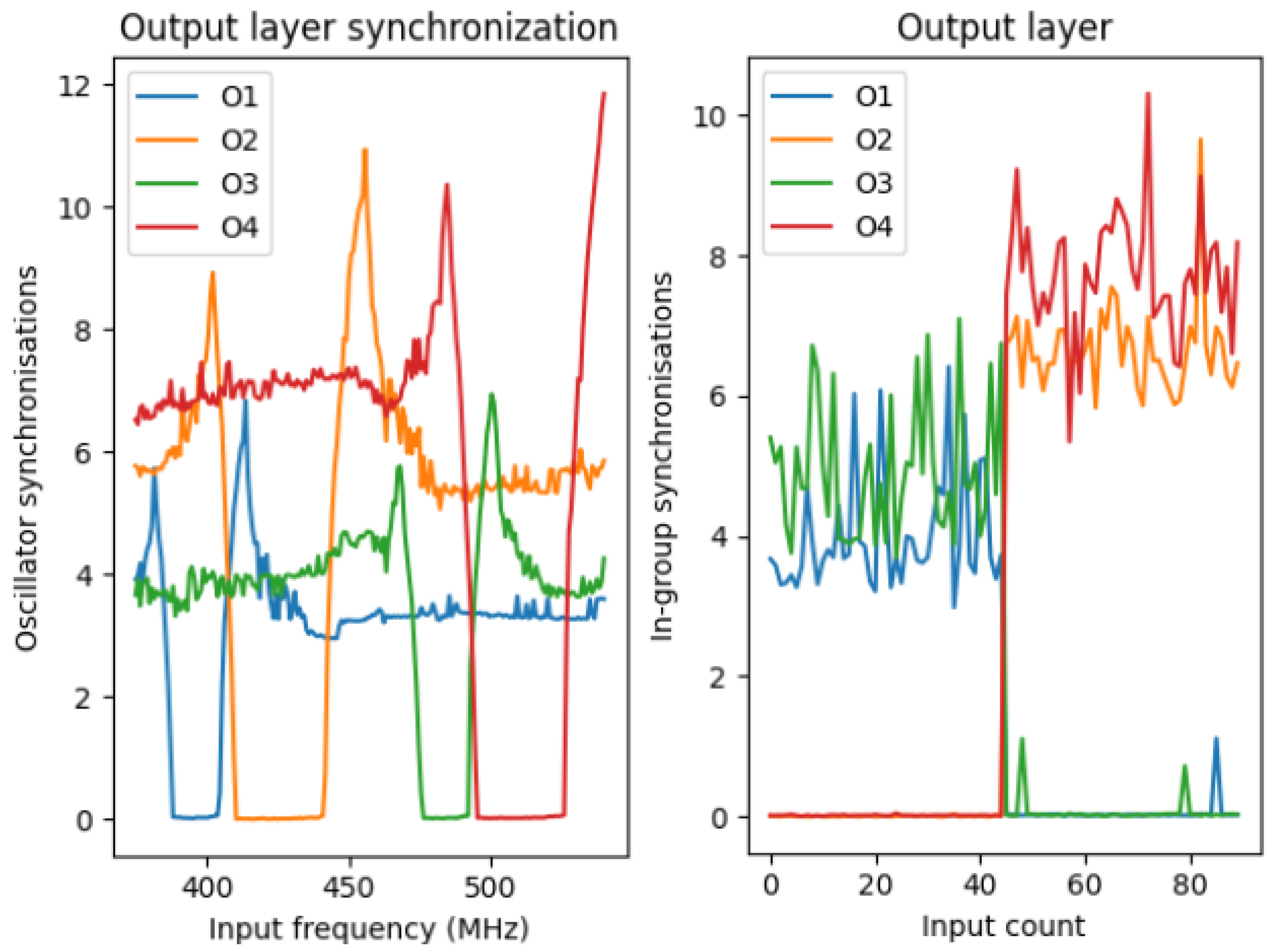
On the left subfigure of Figure 8, the synchronization regions of the two-oscillator groups in the output layer can be seen as dips in the different curves. On the x-axis, there is a sweep of frequencies over an extended range of frequencies, incorporating the frequency ranges of the vowel’s two most dominant frequency components. It can be observed that the O1 and O2 groups are responsible for recognizing the lower frequencies, and the O3 and O4 groups are responsible for the higher frequencies. The synchronization regions do not overlap.
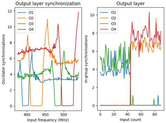
Figure 8.
The left subfigure shows the synchronization value of the 4 pairs of output oscillators. The input sinusoids’ frequency is swept over a given frequency range, and the synchronization appears as a constant part of the well for the curves. On the right side, the same synchronization value can be seen, but it is calculated after feeding the two types of vowels to the system. For the first 45 vowels, being “ah”, O2 and O4 pairs are synchronized, and for the other 45 vowels, being “iy”, the O1 and O3 pairs are synchronized.
In order to measure and algorithmically decide whether any group of oscillators is synchronized or not, we simply used the following formula:
where are the frequencies of the oscillators in the given group. This S value is then scaled and used as a dimensionless number, because the magnitude of this difference is not relevant, just the fact that it is low for synchronizing cases or high for non-synchronizing cases.
On the right subfigure of Figure 8, we can observe the synchronization values of the four oscillator groups in the output layer by the input indices on the x-axis. The first 45 sample was from “iy” vowel and the other 45 sample was from the other, “ah” vowel. It is clear that by using this synchronization metric, the decision is easy. If the sum of the synchronization value of is lower than that of , we can say that it is an “ah” vowel; otherwise, it is an “iy” vowel. It can be seen that for the first batch of samples, the sum of and is close to zero, but the sum of the other two is high; meanwhile, for the other part of the set with the other vowel, it is the other way around.
Also, from this we can conclude that the architecture is capable of solving this task with accuracy.
The physical parameters of the network are summarized in Table 2.
Table 2.
Physical parameters of the resulting system All these parameters were set by trial-and-error and used for the simulations.
In our setup, the frequency difference for the oscillators should be around 20–40 MHz. In this case, a coherent, sinusoidal injected signal can synchronize them. The precise value of the frequency difference depends on the strength of the input; however, the input cannot be overly strong because that would break the oscillatory behavior.
3.1.2. Gradient-Free Optimization of Network Parameters
To eliminate the somewhat heuristic procedure above, we used the Nevergrad package, version 1.0.8, written in Python [23] to let the algorithm figure out the parameters of the network, such as the optimal ring oscillator frequencies.
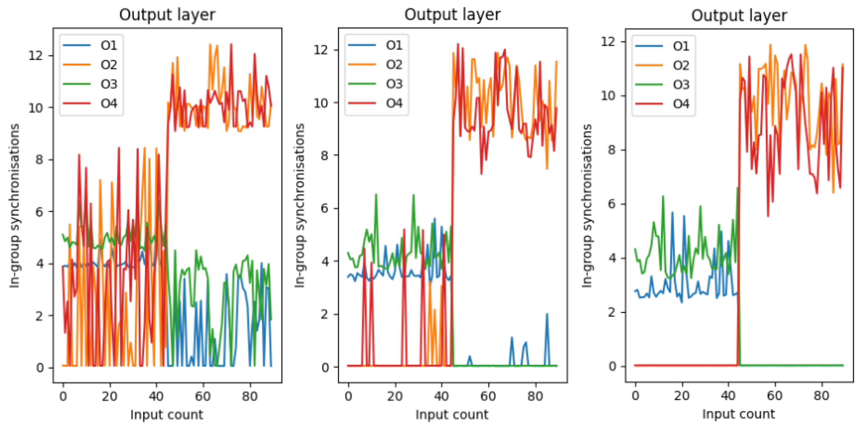
Now, on Figure 9, the same output layer synchronization can be seen at different points in the learning procedure. The left-most figure is the initial state, the middle is an intermediate step during the learning, and the last one is the state where the network learned the separation.
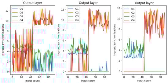
Figure 9.
The synchronization value of the output pairs for the test dataset throughout different stages of learning. The initial state of the left figure is random, then during learning, the synchronization values start to settle to the desired values, and lastly, when the learning is finished, the synchronization values indicate a 100% separation.
For this gradient-free optimization, we used a genetic algorithm to figure out the frequencies and couplings.
The result is very similar to the trial-and-error “by hands” learning as the last state of the learning indicates.
3.2. Recognition of Raw Vowel Waveforms Without Preprocessing
In Figure 4 and in Section 2.6 we demonstrated that applying the vowel waveform directly to the oscillator has a strong effect on its frequency—even if this effect cannot be described as a clean phase and frequency synchronization to an injected signal. However, the frequency correlations between the neighboring oscillators can be picked up using appropriate circuitry.
In order to process raw waveforms, we use a single layer of oscillators with frequencies spanning the spectral range of vowels. Unlike in the network of Section 3.1, we use a small-sized traditional neural network as a second layer to do classification. Oscillators act only as pre-processing layers. The schematic figure of this architecture can be seen in Figure 10.
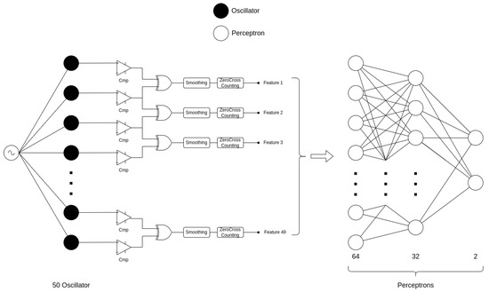
Figure 10.
Mixed architecture for time-domain binary vowel recognition. The first part of the architecture extracts the frequency features of the time-domain vowels by measuring the frequency synchronization strength of neighboring oscillators. The second part uses this feature set as input data to do the actual binary recognition with a simple, multi-layer perceptron architecture.
The first part of the architecture—shown on the left side of Figure 10—is entirely oscillator-based. Its main function is to extract frequency components from the time-domain vowel input by measuring the synchronization strength between neighboring oscillators. Each oscillator’s output voltage is first converted into a binary signal using comparators. Then, the outputs of adjacent oscillators are passed through XOR gates, which operate as follows:
- If two oscillators do not have synchronized frequencies, then the output of their XOR’s duty signal will be constantly changing.
- If two oscillators are synchronized in frequency, then the output of their XOR’s duty signal will be constant over time
The output of the XOR gates passes through a low-pass filter. A circuit can straightforwardly conduct this; in our simulations, we used a moving average filter to emulate its effect.
To create a single feature vector from the time-dependent filtered XOR signal, we can count its zero crossings. Here, if we have a constant duty signal, indicating synchronized oscillators, we will observe fewer zero crossings; otherwise, if the duty signal is constantly changing for two non-synchronizing oscillators, then the number of zero crossings will be high. The detailed changes in the signals coming from the oscillators as output voltages passing through this apparatus are depicted in Figure 11.
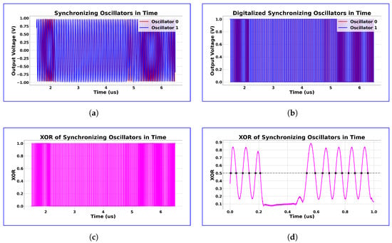
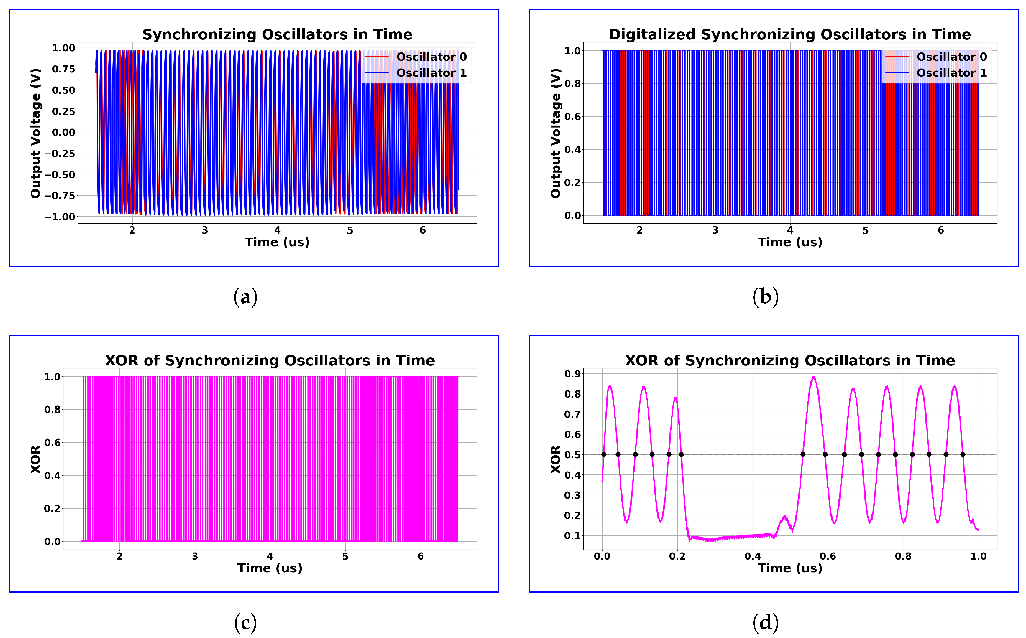
Figure 11.
Transformations on the output signals of two neighboring synchronizing oscillators. The transformations Conducted on the two oscillator signals via the small circuit after the oscillators can be seen on (a–d): (a) output voltages of synchronizing oscillators near the synchronization time frame and it can be observed that in the synchronizing region the two oscillators frequencies are not changing relative to other, but before and after that oscillator 1 is constantly moving over oscillator 0 as the higher frequency oscillator; (b) after digitizing the output signals, two square signal can be observed; (c) the XOR of the synchronizing signals shows similar behavior than (a) as the XOR is changing with constant duty signal in the synchronization region but outside of it the duty signal’s length is constantly changing; (d) after applying a mean filter for the whole XOR signal, we can see the synchronization region clearly and if we count the zero-crossing on this signal we will receive a lower value than we would if this synchronization would not have been present as it can be seen that outside this region the smoothed XOR signal is sinusoid-like. Note that we took the inverse of this value and transformed it to range to achieve the relative signal strength. This way, it is more intuitive to call it synchronization strength.
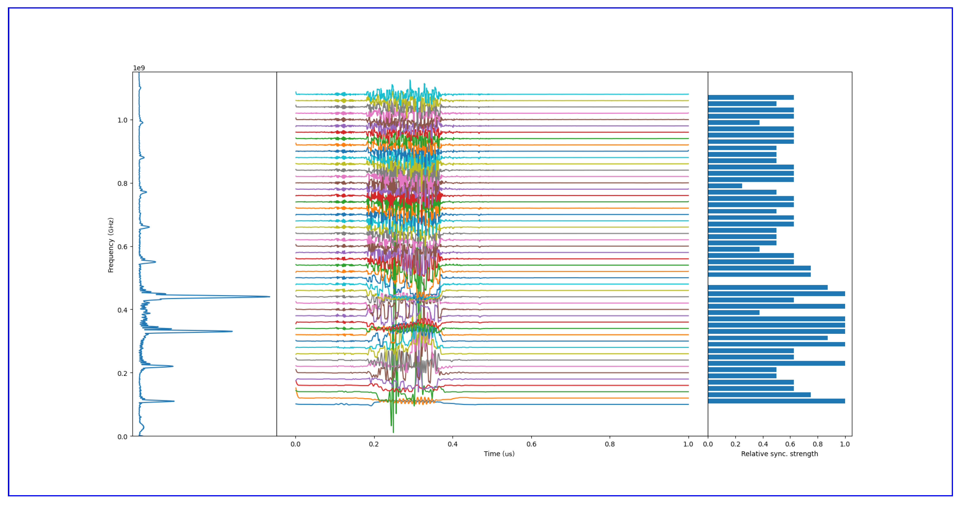
An example showing oscillators react to a time-dependent input, is shown in Figure 12. It is clear from the figure that the oscillators with intrinsic frequencies close to the frequency components in the vowel are synchronized, and the rest are not. On the right, however, we can see the relative frequency synchronization strength between the oscillators. For understanding, the zero crossing values have been normalized to the interval and also they were reversed so that it shows better where the frequency peaks are in the vowel.
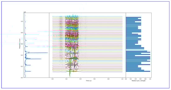
Figure 12.
Example of feature extraction with oscillatory layer. The feature vector element values are high if synchronization is present between two oscillators and low if there is no synchronization, as desired. The frequency spectra of the vowel are on the left, rotated 90 degrees for clarity. The colored curves are the instantaneous frequencies for each oscillator.
We first used the oscillatory architecture to do the feature extraction on the two vowel sets. After that, we used that resulting dataset as an input to the mentioned, low parameter count multi-layer perceptron. It used 49 inputs and 2 outputs with 64 neurons in the first and 32 neurons in the second hidden layer.
Performance on the Dataset
Due to the small dataset and the simple nature of this conventional neural network, the training and evaluation of the architecture are fast.
The confusion matrix of the evaluation of the test set can be observed in Figure 13.
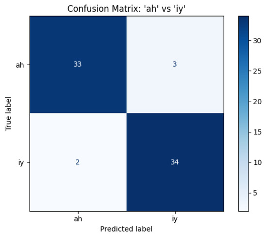
Figure 13.
Confusion matrix of “ah” and “iy” vowels with the mixed architecture. The architecture made some errors, but overall its accuracy is .
Overall, in terms of accuracy, it performed slightly worse than the multi-layered oscillatory network, but that is due to the fact that there the input signals were heavily preprocessed, and here the pre-processing is conducted by the oscillatory layer. Also, do note that the multi-layered perceptron is a very simple network, so it is prone to overfitting, especially for a small dataset we had available.
In terms of the physical parameters here, all the oscillators had the same value for the input resistor and that was k. Here, the remark from the end of Section 3.1.1 is true with the added restriction that the difference between the frequencies of neighboring oscillators should be at most 20–25 MHz, so that 2–4 oscillators could synchronize in frequency to the incoherent input signal for the duration of the speech.
4. Discussion
We presented ONN architectures for processing time-domain vowel signals.
Our first architecture consisted solely of oscillators, but its incoming signals require some preprocessing, which receives formants (coherent oscillatory signals) extracted from the vowels. If the oscillator frequencies are properly chosen, they can achieve a 100% classification accuracy on simple vowels, correctly identifying their frequency constituents.
This way, the classification largely depends on the separability of the formant frequency, especially the two most dominant ones. Although we did manage to reach 100% accuracy for some classes, some performed worse, around 80–90%, depending on the linear separability of the given vowels’ formant frequencies.
A key feature of this network is that it has two oscillator layers; frequency-domain information is passed from the first layer to the second, akin to a feed-forward network. We envision that this architecture can be developed to perform more complex processing functions by making the second layer’s connections more complex.
The second architecture is a single-layered ONN that receives entirely unprocessed signals, i.e., raw waveforms. For the injected broadband signal, a degree of entrainment occurs between the oscillators. This synchronization cannot be passed to another oscillator layer, but can be used to extract a feature vector by means of simple circuitry and further processed by a simple, more conventional neural network.
For this architecture, the accuracy was less than for the first architecture on the test case shown in this paper, but we emphasize that the first approach is using a preprocessed, coherent signal, while this solution is using the pure waveform. Nevertheless, compared with the 100% for the first architecture on “ah” and “iy” vowels, we managed to achieve 93% on the test set, which is high for such a simple circuitry.
Also, we tried a multi-class classification using the second architecture with a 12 output neuron, instead of 2, and we achieved great results on the training set. It reached using a training and validation set, which means that the oscillatory layer managed to extract meaningful information from the raw signals, essentially transforming a time-dependent signal into static data. It should be mentioned, however, that the network was overfitting, failing to generalize to the test set in some cases, which was mainly due to the small amount of samples per class in the test set.
We believe that the overfitting was likely due to the simplicity of the traditional second layer, which is still an extremely simple and lightweight neural network. Work is in progress to optimize the performance of the non-oscillatory layers in the architecture.
The motivation for this work is to achieve ultra-low power signal processing, ring oscillator-based ONNs were shown to outperform the power efficiency of their digital counterparts by two orders of magnitude for simple tasks [8]. Since the ONN we showed that runs at several hundred MHz frequency can perform several ten thousand classifications per second and consists of a few tens of ring oscillators, each of which may consume a mere few microwatts of power [25], the energy cost per inference will fall into nJ per inference regime. This is in line with state-of-the-art hardware classifiers for static data [26] and significantly better than the state of the art for preprocessing-hungry temporal processing.
Oscillatory Neural Networks (ONNs) are most commonly used in image processing tasks, typically as associative memories. In contrast, processing dynamic signals remains a relatively underexplored area—despite ONNs being inherently dynamic systems themselves, making them potentially well-suited for such tasks. We hope that our work encourages further research into the potential of ONNs for dynamic signal processing.
Author Contributions
Conceptualization and funding acquisition: G.C. and W.P. Software, validation data analyzis and concept development: T.R.-H. Writing—original draft preparation: T.R.-H. and G.C. All authors have read and agreed to the published version of the manuscript.
Funding
The author(s) declare financial support was received for the research, authorship, and/or publication of this article. This study was partially supported by a grant from Intel Corporation, titled HIMON: Hierarchically Interconnected Oscillator Networks. This project has received additional funding from the European Union’s Horizon EU research and innovation programme under grant agreement No. 101092096 (PHASTRAC). The funder (Intel Corporation) had the following involvement with the study: helping to discover relevant literature and motivate the study. The funder was not involved in the study design, collection, analysis, interpretation of data, the writing of this article or the decision to submit it for publication.
Institutional Review Board Statement
Not applicable.
Informed Consent Statement
Not applicable.
Data Availability Statement
The authors used the following vowel dataset that can be found at the github link: https://github.com/fancompute/wavetorch, accessed on 1 May 2025, downloaded in 2024 January.
Acknowledgments
The authors are grateful for useful discussions with Amir Khosrowshahi, Narayan Srinivasa and Dmitri Nikonov—all at that time at Intel Corporation.
Conflicts of Interest
The authors declare no conflicts of interest.
References
- Csaba, G.; Porod, W. Coupled oscillators for computing: A review and perspective. Appl. Phys. Rev. 2020, 7, 011302. [Google Scholar] [CrossRef]
- Todri-Sanial, A.; Delacour, C.; Abernot, M.; Sabo, F. Computing with oscillators from theoretical underpinnings to applications and demonstrators. npj Unconv. Comput. 2024, 1, 14. [Google Scholar] [CrossRef] [PubMed]
- Vadlamani, S.K.; Xiao, T.P.; Yablonovitch, E. Combinatorial optimization using the Lagrange primal-dual dynamics of parametric oscillator networks. Phys. Rev. Appl. 2024, 21, 044042. [Google Scholar] [CrossRef]
- Chou, J.; Bramhavar, S.; Ghosh, S.; Herzog, W. Analog coupled oscillator based weighted Ising machine. Sci. Rep. 2019, 9, 14786. [Google Scholar] [CrossRef] [PubMed]
- Hoppensteadt, F.C.; Izhikevich, E.M. Pattern recognition via synchronization in phase-locked loop neural networks. IEEE Trans. Neural Netw. 2000, 11, 734–738. [Google Scholar] [CrossRef] [PubMed]
- Velichko, A.A.; Ryabokon, D.V.; Khanin, S.D.; Sidorenko, A.V.; Rikkiev, A.G. Reservoir computing using high order synchronization of coupled oscillators. In IOP Conference Series: Materials Science and Engineering; IOP Publishing: Bristol, UK, 2020; Volume 862, p. 052062. [Google Scholar]
- Shamsi, J.; Avedillo, M.J.; Linares-Barranco, B.; Serrano-Gotarredona, T. Oscillatory Hebbian Rule (OHR): An adaption of the Hebbian rule to Oscillatory Neural Networks. In Proceedings of the 2020 XXXV Conference on Design of Circuits and Integrated Systems (DCIS), Segovia, Spain, 18–20 November 2020; pp. 1–6. [Google Scholar]
- Rudner-Halász, T.; Porod, W.; Csaba, G. Design of oscillatory neural networks by machine learning. Front. Neurosci. 2024, 18, 1307525. [Google Scholar] [CrossRef] [PubMed]
- Scellier, B.; Bengio, Y. Equilibrium propagation: Bridging the gap between energy-based models and backpropagation. Front. Comput. Neurosci. 2017, 11, 24. [Google Scholar] [CrossRef] [PubMed]
- Laydevant, J.; Marković, D.; Grollier, J. Training an ising machine with equilibrium propagation. Nat. Commun. 2024, 15, 3671. [Google Scholar] [CrossRef] [PubMed]
- Wang, Q.; Wanjura, C.C.; Marquardt, F. Training coupled phase oscillators as a neuromorphic platform using equilibrium propagation. Neuromorph. Comput. Eng. 2024, 4, 034014. [Google Scholar] [CrossRef]
- Cetin, O. Accent recognition using a spectrogram image feature-based convolutional neural network. Arab. J. Sci. Eng. 2023, 48, 1973–1990. [Google Scholar] [CrossRef]
- Romera, M.; Talatchian, P.; Tsunegi, S.; Abreu Araujo, F.; Cros, V.; Bortolotti, P.; Trastoy, J.; Yakushiji, K.; Fukushima, A.; Kubota, H.; et al. Vowel recognition with four coupled spin-torque nano-oscillators. Nature 2018, 563, 230–234. [Google Scholar] [CrossRef] [PubMed]
- Zhong, Y.; Tang, J.; Li, X.; Gao, B.; Qian, H.; Wu, H. Dynamic memristor-based reservoir computing for high-efficiency temporal signal processing. Nat. Commun. 2021, 12, 408. [Google Scholar] [CrossRef] [PubMed]
- Nikonov, D.E.; Csaba, G.; Porod, W.; Shibata, T.; Voils, D.; Hammerstrom, D.; Young, I.A.; Bourianoff, G.I. Coupled-oscillator associative memory array operation for pattern recognition. IEEE J. Explor. Solid-State Comput. Devices Circ. 2015, 1, 85–93. [Google Scholar] [CrossRef]
- Vassilieva, E.; Pinto, G.; de Barros, J.; Suppes, P. Learning Pattern Recognition Through Quasi-Synchronization of Phase Oscillators. IEEE Trans. Neural Netw. 2011, 22, 84–95. [Google Scholar] [CrossRef] [PubMed]
- Crook, S.M.; Ermentrout, G.B.; Bower, J.M. Spike Frequency Adaptation Affects the Synchronization Properties of Networks of Cortical Oscillators. Neural Comput. 1998, 10, 837–854. [Google Scholar] [CrossRef] [PubMed]
- Taylor, D.; Ott, E.; Restrepo, J.G. Spontaneous synchronization of coupled oscillator systems with frequency adaptation. Phys. Rev. E 2010, 81, 046214. [Google Scholar] [CrossRef] [PubMed]
- Csaba, G.; Ytterdal, T.; Porod, W. Neural network based on parametrically-pumped oscillators. In Proceedings of the 2016 IEEE International Conference on Electronics, Circuits and Systems (ICECS), Monte Carlo, Monaco, 11–14 December 2016; IEEE: Piscataway, NJ, USA, 2016; pp. 45–48. [Google Scholar]
- Pikovsky, A.; Rosenblum, M.; Kurths, J. Synchronization: A Universal Concept in Nonlinear Sciences; Cambridge University Press: Cambridge, UK, 2001. [Google Scholar]
- Hughes, T.W.; Williamson, I.A.; Minkov, M.; Fan, S. Wave physics as an analog recurrent neural network. Sci. Adv. 2019, 5, eaay6946. [Google Scholar] [CrossRef] [PubMed]
- Chen, R.T.Q. torchdiffeq GitHub Repository. 2018. Available online: https://github.com/rtqichen/torchdiffeq (accessed on 1 May 2025).
- Rapin, J.; Teytaud, O. Nevergrad-A Gradient-Free Optimization Platform. GitHub Repository. 2018. Available online: https://GitHub.com/FacebookResearch/Nevergrad (accessed on 1 May 2025).
- Paszke, A.; Gross, S.; Chintala, S.; Chanan, G.; Yang, E.; DeVito, Z.; Lin, Z.; Desmaison, A.; Antiga, L.; Lerer, A. Automatic differentiation in pytorch. In Proceedings of the 31st Conference on Neural Information Processing Systems (NIPS 2017), Long Beach, CA, USA, 4–9 December 2017. [Google Scholar]
- Ballo, A.; Pennisi, S.; Scotti, G.; Venezia, C. A 0.5 V sub-threshold CMOS current-controlled ring oscillator for IoT and implantable devices. J. Low Power Electron. Appl. 2022, 12, 16. [Google Scholar] [CrossRef]
- Tunheim, S.A.; Zheng, Y.; Jiao, L.; Shafik, R.; Yakovlev, A.; Granmo, O.C. An All-digital 65-nm Tsetlin Machine Image Classification Accelerator with 8.6 nJ per MNIST Frame at 60.3 k Frames per Second. arXiv 2025, arXiv:2501.19347. [Google Scholar]


Disclaimer/Publisher’s Note: The statements, opinions and data contained in all publications are solely those of the individual author(s) and contributor(s) and not of MDPI and/or the editor(s). MDPI and/or the editor(s) disclaim responsibility for any injury to people or property resulting from any ideas, methods, instructions or products referred to in the content. |
© 2025 by the authors. Licensee MDPI, Basel, Switzerland. This article is an open access article distributed under the terms and conditions of the Creative Commons Attribution (CC BY) license (https://creativecommons.org/licenses/by/4.0/).