Article

Leveraging Degradation Events for Enhanced Remaining Useful Life Prediction

by
Zeeshan Abbas
1,
Muhammad Sharif
2,
Musrat Hussain
3,
Naeem Hussain
1,
Mehboob Hussain
4,* and
Naveed Ahmad Khan
5
1
College of Electronics and Information Engineering, Shenzhen University, Shenzhen 518060, China
2
State Key Laboratory of Multimodal Artificial Intelligence Systems, Beijing 100190, China
3
Shenzhen Institutes of Advanced Technology, Chinese Academy of Sciences, Shenzhen 518060, China
4
School of Information Science and Technology, Southwest Jiaotong University, Chengdu 611756, China
5
School of Information Technology and Information Systems, University of Canberra, Canberra, ACT 2617, Australia
*
Author to whom correspondence should be addressed.
Information 2025, 16(7), 542; https://doi.org/10.3390/info16070542
Submission received: 23 April 2025 / Revised: 2 June 2025 / Accepted: 17 June 2025 / Published: 26 June 2025

Abstract

The remaining useful life (RUL) of complex mechanical systems is the primary aspect of prognostics and health management, which is critical for ensuring reliability and safety. Recent developments have shifted towards a data-driven approach, emphasizing empirical insights over expert opinions. The similarity-based data-driven approach operates on the premise that systems with similar historical behaviors will likely exhibit similar future behaviors, making it suitable for RUL estimation. Conventionally, most similarity-based approaches utilize all historical data to identify reference systems for RUL estimations. However, not all historical events within a system hold equal significance for RUL. Certain events have a substantial impact on the remaining lifespan of a system. These significant and impactful events are called degradation events (DEs) in this study. Based on the hypothesis that systems undergoing similar DEs may share the same RUL, this study presents an innovative framework for RUL estimation that leverages only the DEs of a test system to identify reference systems that have experienced similar DEs. Furthermore, the model incorporates novel strategies for adjusting the RUL of the reference system based on the initial wear and degradation rates, thereby improving estimation accuracy. The effectiveness of the proposed model, in comparison with similar state-of-the-art models, is demonstrated through experiments on widely recognized jet engine datasets provided by NASA and bearing degradation data from the XJTU-SY.

1. Introduction

Industrial systems, especially those operating in safety-critical domains such as aerospace, manufacturing, energy, and transportation, are susceptible to performance degradation and failure due to wear, environmental stressors, and unexpected operational anomalies. Such failures can result in significant safety hazards, production losses, and maintenance costs. As a result, prognostics and health management (PHM) has emerged as a key area of research focused on improving system reliability and maintainability by enabling early detection of faults and precise estimation of the remaining useful life (RUL) of components [1,2,3,4,5,6].
A fundamental challenge in PHM is the accurate prediction of RUL using historical and real-time monitoring data, such as sensor signals that reflect system health. Timely and precise RUL estimation facilitates predictive maintenance, which prevents unexpected failures, reduces life-cycle costs, and enhances operational efficiency [7,8]. RUL estimation methods can be broadly categorized into model-driven and data-driven approaches [9,10].
Model-driven methods rely on physics-based degradation models, damage accumulation laws, or empirical formulations to describe the progression of wear and tear [11,12]. While effective in systems where physical degradation mechanisms are well understood, these approaches often suffer from limited generalizability due to system complexity, heterogeneity, and the lack of detailed domain-specific knowledge.
In contrast, data-driven methods have shown significant promise by learning degradation patterns directly from sensor data without requiring explicit physical models [13,14,15]. Techniques based on machine learning, deep learning, and signal similarity have been extensively studied. However, many data-driven models act as “black boxes,” offering limited interpretability—an essential consideration in mission-critical systems. Furthermore, these approaches often assume that all segments of sensor data are equally informative, overlooking localized degradation indicators.
Similarity-based RUL estimation methods have attracted interest among data-driven techniques due to their relatively high interpretability. These methods operate on the assumption that systems exhibiting similar historical behavior are likely to experience similar future outcomes [9]. Depending on the granularity of the similarity search, these can be classified into global and local similarity-based approaches [2,16]. Global similarity techniques use the entire historical trajectory of the system up to a given time, which can be impractical when operational environments vary or when degradation behavior diverges significantly over time. Local similarity approaches address this by comparing short-time segments (subsequences) using sliding windows but often suffer from computational inefficiency and fail to prioritize critical degradation patterns. The local similarity-based approaches assume that all subsequences in sensor data contribute equally to degradation modeling, as illustrated in Figure 1a. In practice, systems such as roller bearings or aircraft engines often experience degradation events (DEs)—characterized by abrupt, anomalous sensor behavior—that carry more diagnostic significance than stable operational patterns. Ignoring these events may lead to suboptimal RUL estimation and inefficient training.
To overcome these limitations, we propose a novel degradation event-aware RUL estimation framework (DERUL). The core idea of DERUL is to prioritize segments of sensor data that exhibit strong degradation patterns by dynamically identifying DEs, as illustrated in Figure 1b. These DEs are then used to guide the similarity-based matching process, improving the efficiency and accuracy of RUL estimation. Unlike prior methods that rely on fixed thresholds for anomaly detection or exhaustive similarity computations across all subsequences, DERUL employs an adaptive strategy for DE extraction and focuses the similarity search on the most informative segments.
The proposed DERUL framework addresses this limitation by dynamically identifying DEs based on abrupt variations in the historical data of each engine rather than relying on predefined thresholds. As illustrated in Figure 1a, DERUL confines the similarity search to dynamically extracted DEs, thereby significantly reducing computational complexity. This event-focused strategy is particularly effective in applications such as roller bearings and turbofan engine degradation, where sudden changes in sensor signals serve as strong indicators of impending failure. By prioritizing these critical segments, DERUL enhances the accuracy and efficiency of RUL estimation, offering a practical solution for real-world applications.
DERUL leverages a motif-based reference system selection technique and includes adjustment strategies for initial wear and degradation rates, further refining the RUL estimates. The framework is validated on benchmark datasets such as C-MAPSS- and XJTU-SY-bearing datasets [17,18], demonstrating superior performance compared with several state-of-the-art baselines.
The primary contributions of this study are summarized as follows:
  • We introduce a degradation event-based approach that prioritizes abrupt sensor variations (DEs), improving both interpretability and performance in RUL estimation.
  • We propose a motif-based reference selection technique that eliminates unnecessary comparisons, reducing computational cost while preserving accuracy.
  • To make the reference RUL more appropriate, we proposed the initial wear-based adjustment and degradation rate-based adjustment strategies.
  • An end-to-end DERUL framework is proposed and evaluated on C-MAPSS and XJTU datasets, outperforming several competitive RUL estimation models.
The remainder of this paper is organized as follows: The literature review is presented in Section 2. Section 3 introduces the framework of DERUL, encompassing preliminary data preprocessing, extraction of DEs, utilization of the extracted DEs for effective system selection, and RUL adjustment strategies to refine the reference RUL. Section 4 assesses the proposed framework and summarizes the experimental evaluation. Finally, Section 5 outlines the future work and concludes the paper.

2. Literature Review

Similarity-based methods are generally categorized into two primary classes: global similarity-basedand local similarity-based approaches [2].

2.1. Global Similarity-Based Approaches

Global approaches consider the entire operational history of a test unit—up to the prediction point—to identify similar historical trajectories [9,16]. For instance, Ref. [9] proposed a degradation-degree-based RUL estimation method that clusters degradation patterns into slow and fast groups. However, these approaches often struggle in real-world scenarios due to environmental variability and operational disturbances. Systems with similar early-stage degradation patterns may diverge significantly, leading to unreliable RUL predictions. Furthermore, the likelihood of finding similar reference systems globally is typically low, limiting the method’s robustness and scalability.

2.2. Local Similarity-Based Approaches

To address the limitations of global similarity-based approaches, local similarity-based methods compare short segments (subsequences) of sensor data between test and reference units [2,19,20]. A sliding window mechanism is typically employed to extract subsequences of length W with step size S, followed by pairwise similarity computations. Ref. [19] introduced a trajectory similarity-based RUL prediction method using adaptive kernel density estimation. However, their framework was restricted to a single prediction point. Ref. [2] extended this by segmenting health indicators into local trajectories and introduced a coarse-to-fine similarity search to reduce computational complexity.
While local methods improve flexibility and scalability, most assume that all subsequences carry equal prognostic value. This assumption can be misleading, particularly in systems where degradation manifests as sudden and abnormal variations in sensor data—referred to as DEs. These DEs, such as spikes in vibration or temperature data, are often more informative than routine signals and correlate strongly with system failures.

2.3. Event-Aware RUL Estimation Methods
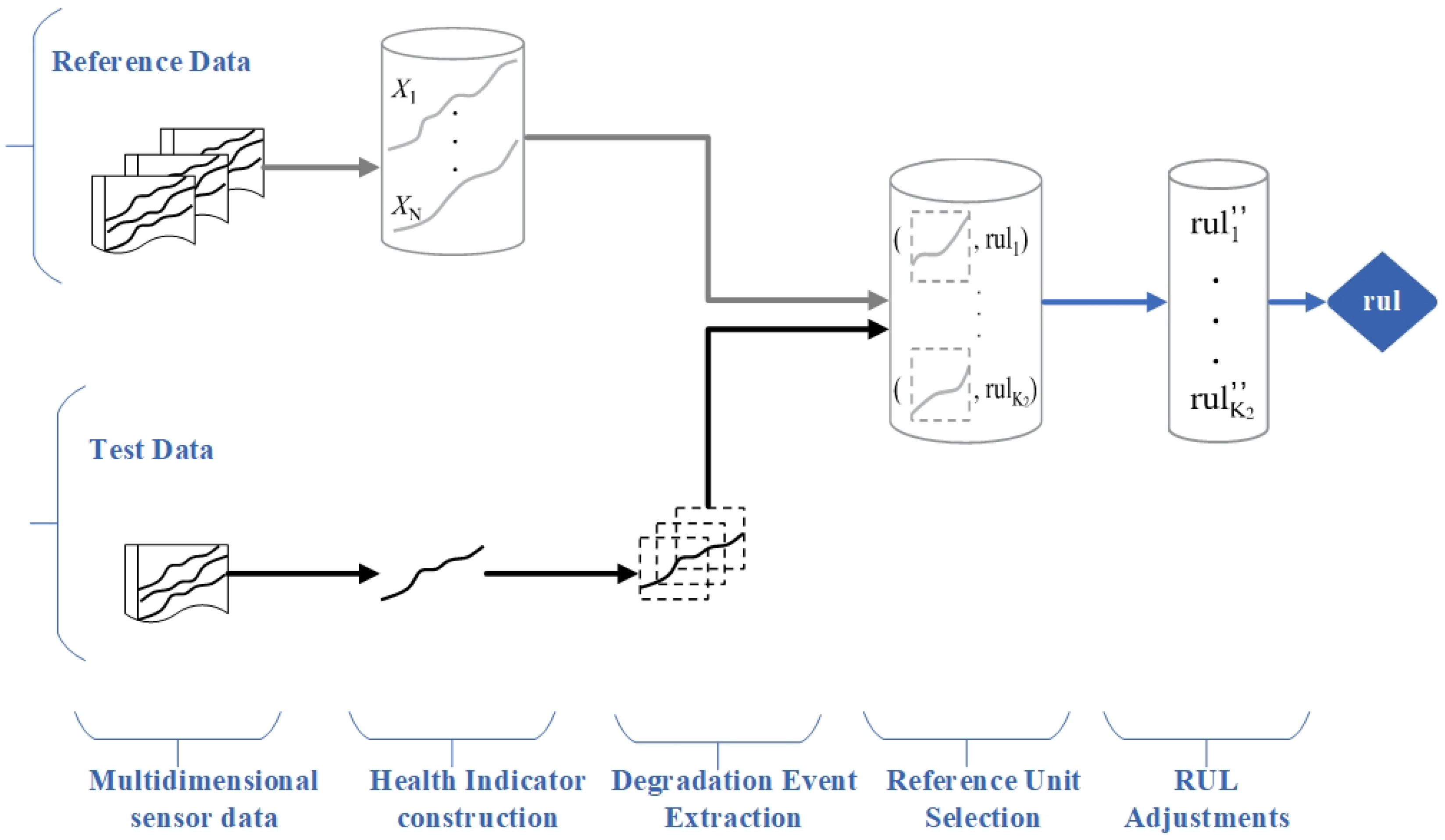
Recent studies have addressed the importance of identifying critical events in time series data. Ref. [21] proposed an anomaly-triggered RUL estimation framework that first detects anomalies and then predicts RUL. However, their use of static thresholds for anomaly detection undermines generalizability across systems with diverse degradation profiles.
To overcome this, we propose the DERUL framework. DERUL dynamically identifies DEs from the historical data of each engine or subsystem, eliminating the need for static thresholds. The approach significantly reduces computational complexity while enhancing prediction accuracy by restricting similarity matching to DE-containing subsequences.
Figure 1 illustrates the conceptual difference between traditional local similarity and the proposed DE-based mechanism. In contrast with comparing all subsequences, DERUL focuses only on high-impact segments with abnormal characteristics, offering a more targeted and efficient RUL estimation method.

3. Methodology

The proposed DERUL is a system-level approach for estimating the RUL of a system. The proposed framework estimates the RUL of the test system by utilizing the run-to-failure history of the available reference datasets. The proposed DERUL framework is outlined in Algorithm 1, and its dataflow diagram is illustrated in Figure 2. The DERUL consists of three key components: (i) construction of a health indicator from multivariate sensor readings, (ii) detection of significant degradation events (DEs) from the test system using the matrix profile, and (iii) similarity-based reference systems based on DE-to-trajectory comparisons and RUL adjustments.
Algorithm 1 DERUL algorithm.
Require: 
A test system T t e s t , a set of reference systems Dataset T , and an integer K are used to specify how many similar references will be selected.
Ensure: 
The predicted RUL r u l ^ of the test system is given by
  1:
HI ;
  2:
RUL r e f ;
  3:
for each T i in T  do
  4:
     H I i H I C o n s t r u c t i o n ( T i ) ;
  5:
     HI HI H I i
  6:
end for
  7:
H I t e s t H I C o n s t r u c t i o n ( T t e s t ) ;
  8:
D E t e s t D E E x t r a c t i o n ( H I t e s t ) ;
  9:
S r e f S i m R e f U n i t ( HI , D E t e s t , K ) ;
10:
for each S r e f in S r e f  do
11:
      R U L r e f * I n i t i a l W e a r A d j u s t ( S r e f , T t e s t ) ;
12:
      R U L r e f * * R a t e B a e d A d j u s t ( R U L r e f * , S r e f , T t e s t ) ;
13:
      RUL r e f RUL r e f R U L r e f * * ;
14:
end for
15:
RUL ;
16:
for each R U L r e f in RUL r e f  do
17:
      ω W e i g h t A s s i g n m e n t ( R U L r e f , T p r e d ) ;
18:
      RUL RUL ( ω , R U L r e f ) ;
19:
end for
20:
r u l ^ K e r n e l D e n s i t y E s t i m a t i o n ( RUL ) ;
21:
return r u l ^ ;

3.1. Health Indicator Construction

The Internet of Things (IoT) ecosystem, comprising sensors, controllers, and intelligent monitoring devices, generates multivariate time-series data X R T × d , where T is the number of observations and d is the number of sensors. While these multidimensional signals contain critical health information, their direct utilization for condition monitoring presents computational challenges due to the curse of dimensionality.
Following [2], we construct a health indicator (HI) through principal component analysis (PCA), which provides an optimal linear projection for dimensionality reduction. The HI is specifically derived from the first principal component (PC1), which captures the dominant mode of variation in the sensor data, as follows:
HI t = X t w 1 ,
where w 1 is the eigenvector corresponding to the largest eigenvalue of the covariance matrix Σ = E [ X X ] . For each equipment instance, we obtain an HI trajectory, as follows:
HI ( i ) = { HI t ( i ) } t = 1 T
The complete system health representation consists of N such trajectories, as follows:
HI = { HI ( i ) } i = 1 N
The proportion of variance explained by PC1, given by λ 1 / i = 1 d λ i where { λ i } are the eigenvalues of Σ , quantifies the information retained in this compressed representation.

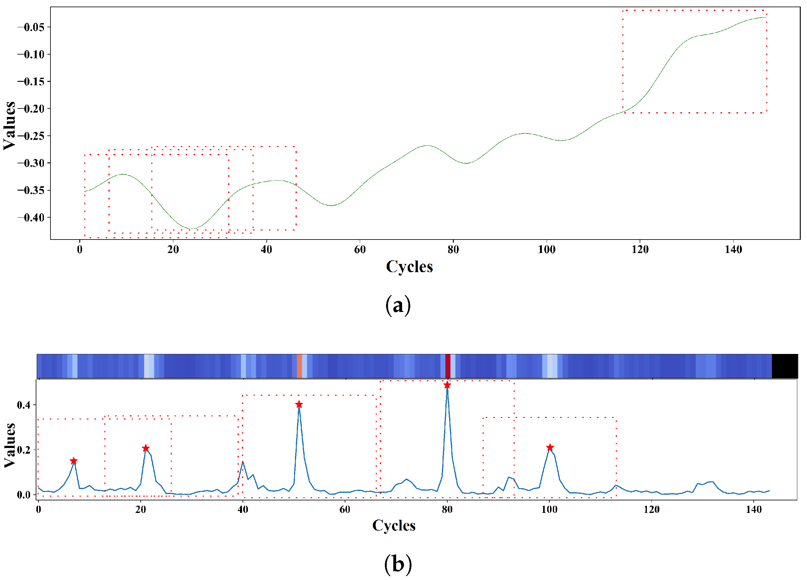
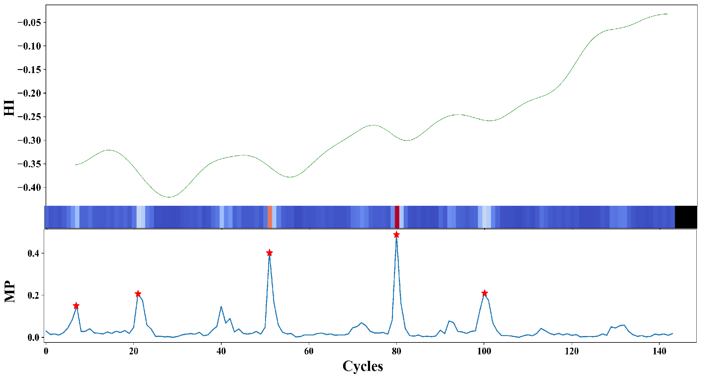
3.2. Degradation Event Extraction Using Matrix Profile

The primary objective of the proposed approach is to identify specific events that represent the degradation of a test system. When a test system undergoes states similar to those already experienced by a reference system, it implies that such events do not occur accidentally. Consequently, they are essential indicators for RUL estimation and are called “degradation events” in the proposed framework.
Extracting DEs is particularly challenging in the absence of comprehensive knowledge of the underlying physical degradation mechanisms. The simplest method for detecting DEs is to use labeled data. Given the labeled data for DEs, the problem can typically be addressed using binary classification. However, in most practical systems, labeled datasets of DEs are not available. Consequently, we employed the matrix profile to extract the DEs. Before extracting DEs, it is necessary to provide a concise explanation of the calculation methods for the distance profile and matrix profile.

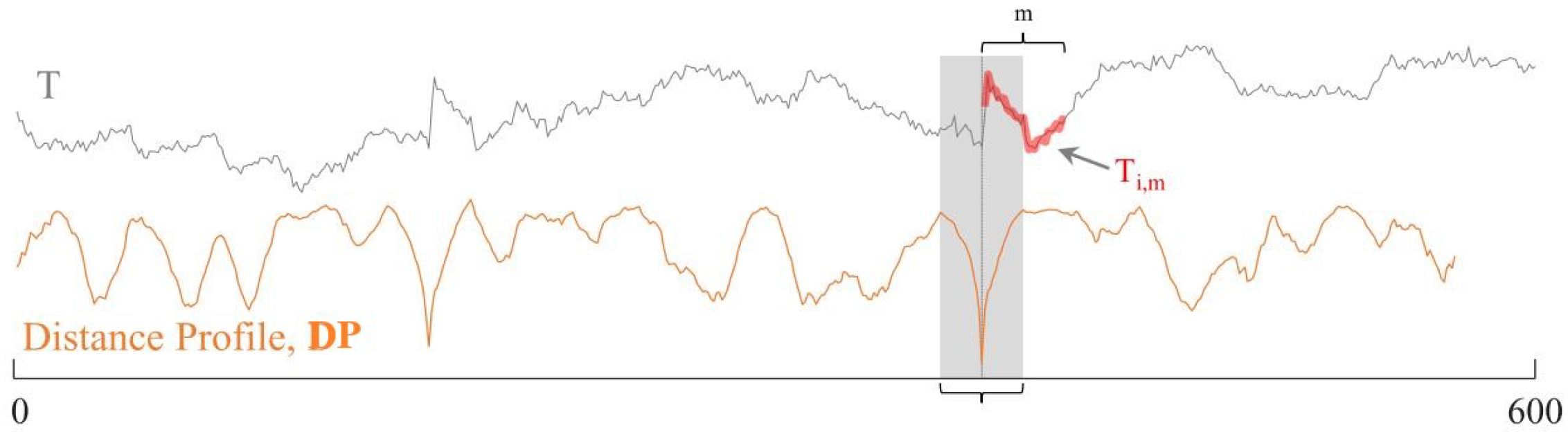
3.2.1. Distance Profile

Definition 1.
A distance profile ( D P ) is a z-normalized Euclidean distance vector representing the similarity between a subsequence or query and all subsequences in the set S of a time series T.
The pairwise z-normalized Euclidean distances between a query (or subsequence) and all-time series subsequences are evaluated to compute the distance profile. The distance profile, denoted as D P , for a time series T and a subsequence S, is represented as a vector of distances, which can be defined as
D P = D 1 , , D q s . t . D j = 1 n i = 1 n ( S ) T j + i 1 S i 2 j = 1 , , q ,
where q = ( n m ) + 1 .
“All-subsequences” can be defined as a set of subsequences derived from a time series that encompasses all possible combinations. This “all-subsequences” concept is primarily used for notation. The implementation refrains from extracting all subsequences because of its exponential time complexity and potential memory constraints. Figure 3 illustrates the distance profile of the time series T with a subsequence T ( i , m ) .
The computed distance profile should be zero at the query or subsequence T ( i , m ) and approach zero in proximity immediately before and after the subsequence T ( i , m ) . Matches that closely approximate zero are referred to as trivial. Typically, these trivial matches are avoided by skipping the exclusion zone of | m | / 2 before and after the index of T ( i , m ) , which is highlighted by the gray region in Figure 3.

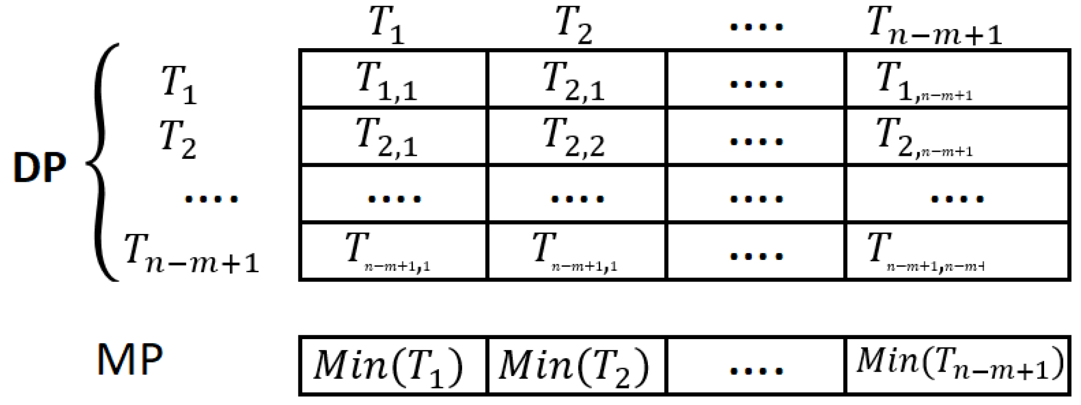
3.2.2. Matrix Profile

Definition 2.
A matrix profile M P is the smallest non-trivial distance from the distance profile D P [1].
Here, we provide a concise exploration of the matrix profile. The matrix profile is a meta-vector encompassing the time series and corresponding z-normalized Euclidean distances for all subsequences and their nearest neighbors. We only extracted the smallest non-trivial distances from the distance profile for the matrix profile.
The matrix profile vector also annotates several exploitable and noteworthy properties. For instance, the highest variation in the profile corresponds to a fault or discord in the time series, which can be interpreted as a DE. The matrix profile, denoted as M P , for a time series T is represented as a vector, where M P j signifies the j-th value, representing the distance between the subsequence T ( i , m ) and its closest subsequence T ( i , m ) , with the minimum distance M P ( T ( j , l ) ) without considering T ( i , j ) aligned with itself at position j, as follows:
M P = M 1 , , M q s . t . M j = min M P T j , l j = 1 , , q j j j = 1 , , q
The relationship between the matrix and distance profiles is depicted in Figure 4.
The primary objective of this study is to identify DEs from the set of all-subsequences S . To this end, we define it from various perspectives. According to [22], there is a subtle variation in the dynamics of sensor data (e.g., a sudden faster degradation) when a fault or degradation occurs in the system. Consequently, our initial definition is based on the degradation rate.
Definition 3
(Degradation Rate-Based). A degradation event D is the maximally representative subsequence, which exhibits the highest change value in the degradation rate within the set of all subsequences  S .
As per [23], standard sensor data tend to be more abundant than degradation data. Therefore, the second definition can be based on the frequency of occurrence.
Definition 4
(Occurrence-Based). A degradation event D has a maximum discrepancy among all subsequences S .
A DE is an occurrence caused by an anomaly or fault, albeit less severe, and does not result in abrupt failure. Therefore, we can define DE from an anomaly perspective.
Definition 5
(Anomaly-Type). A degradation event D is a minor anomaly or fault that does not lead to a sudden failure. Instead, it provides early warnings of potential system faults, thereby reducing the RUL of the systems.
The matrix profile is a time series that annotates several exploitable and intriguing properties. For instance, the highest variation in the profile corresponds to a fault or discord in the time series, which is considered a DE. This definition aligns with all provided Definitions 3–5.
A significant distinction from other related approaches [21] is that we do not assume any threshold value. Every engine has unique characteristics and operates under different conditions; therefore, applying a fixed threshold across all engines is not feasible. To overcome this limitation, DERUL dynamically selects DEs based on the top k highest values within each engine’s historical data to ensure that minor DEs are not overlooked. The algorithm for extracting DEs is presented in Algorithm 2. The vertical dashed line in Figure 5 represents the approximate center of the DE from the HI trajectory. It satisfies all definitions, including Definitions 3–5.
Algorithm 2 Degradation event extraction.
Require: 
A set of test systems H I t e s t .
Ensure: 
Degradation event D E .
  1:
M P M a t r i x P r o f i l e ( H I t e s t ) ;
  2:
D E M a x ( k , M P )
  3:
return DE

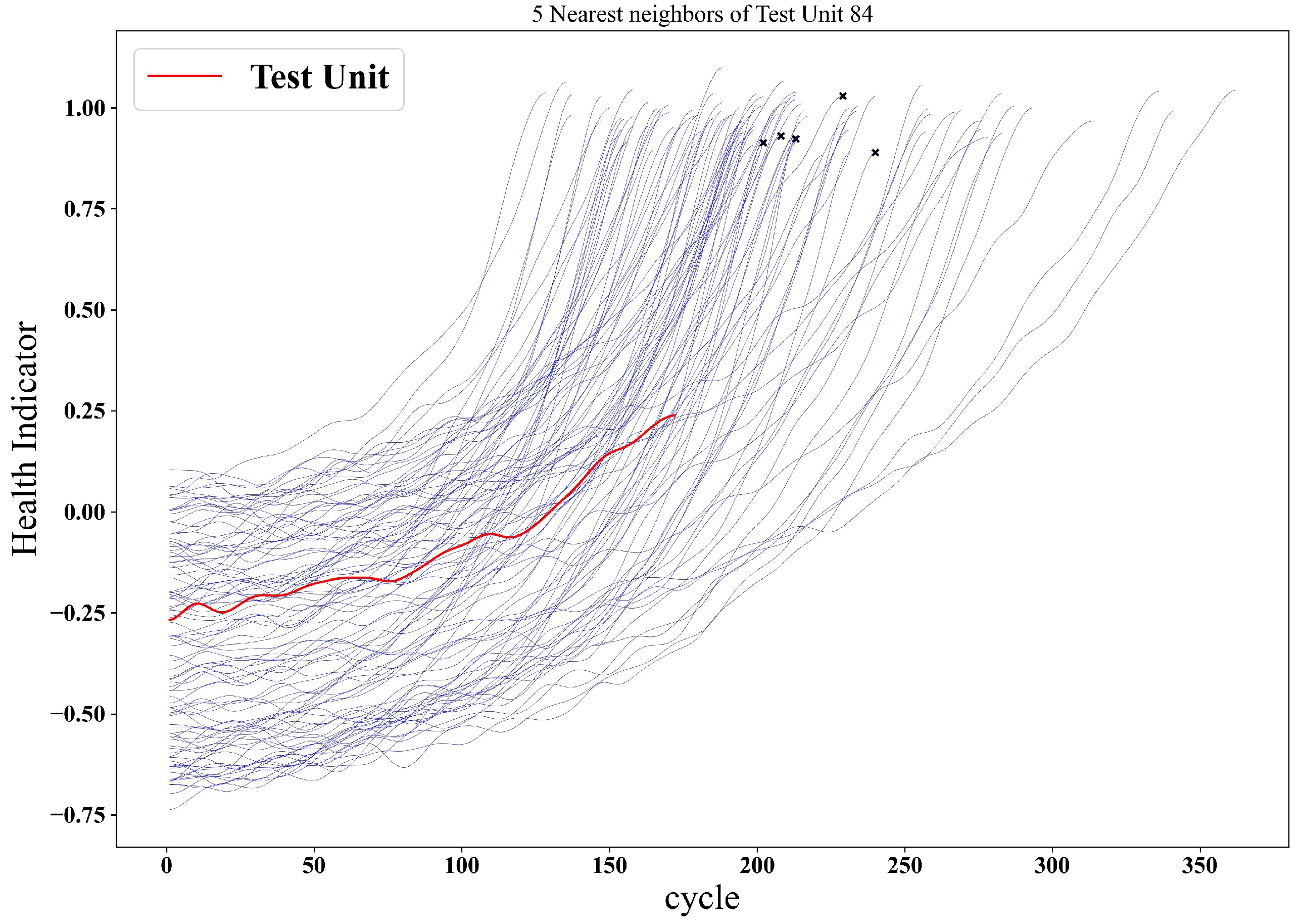
3.3. Reference System Selection

The primary objective of this study was to investigate the influence of DEs on the RUL of a system. After extracting DEs from the test system, the next step is to leverage these events to identify the most suitable reference system.
D P = D 1 , , D q s . t . D j = 1 n i = 1 n ( S ) T j + i 1 D E 2 j = 1 , , q ,
where q = ( n m ) + 1 .
Unlike in the traditional distance profile in Section 3.2.1 and the matrix profile in Section 3.2.2, we are interested in finding reference systems with the most similar DE to the test system. As shown in Figure 6a, the lowest distance of the matrix profile represents the most similar subsequence to the test DE of the test system with an extracted DE, which is considered alongside two reference systems exhibiting subsequences resembling the test DE in Figure 6b. The reference system displaying the closest resemblance to the DE of the test system is chosen to estimate the RUL of the test system. Specifically, r e f 1 manifests a subsequence more similar to the test DE than r e f 2 .
Since the distance profile contains the pairwise list of z-normalized Euclidean distances D P between the degradation event D E and every subsequence of the reference system, the smallest non-trivial distance values, along with their positional indices, constitute the matrix profile. Reference systems with subsequences most similar to the extracted DEs were chosen for the RUL estimation. In other words, the smallest value from the matrix profile signifies the most similar subsequences, which can be obtained using Algorithm 3.
Algorithm 3 Motif-based reference selection.
Require: 
A test system’s degradation event D E and a set of reference systems HI .
Ensure: 
Top K selected the reference system for the RUL estimation.
  1:
MP
  2:
for each H I in HI  do
  3:
     MP M a t r i x P r o f i l e ( H I , D E )
  4:
end for
  5:
return M i n ( k , MP )
Algorithm 3 requires a set of all known reference systems denoted as HI and the degradation event D E of a test system. The algorithm locates the motif (the most similar subsequence) in each reference system that closely resembles the test system’s D E . The reference system with the most similar motif to the test system’s D E is prioritized in arranging the reference systems within the set HI . From the sorted reference systems in HI , the algorithm returns the top k reference systems, which are subsequently utilized for RUL estimation.

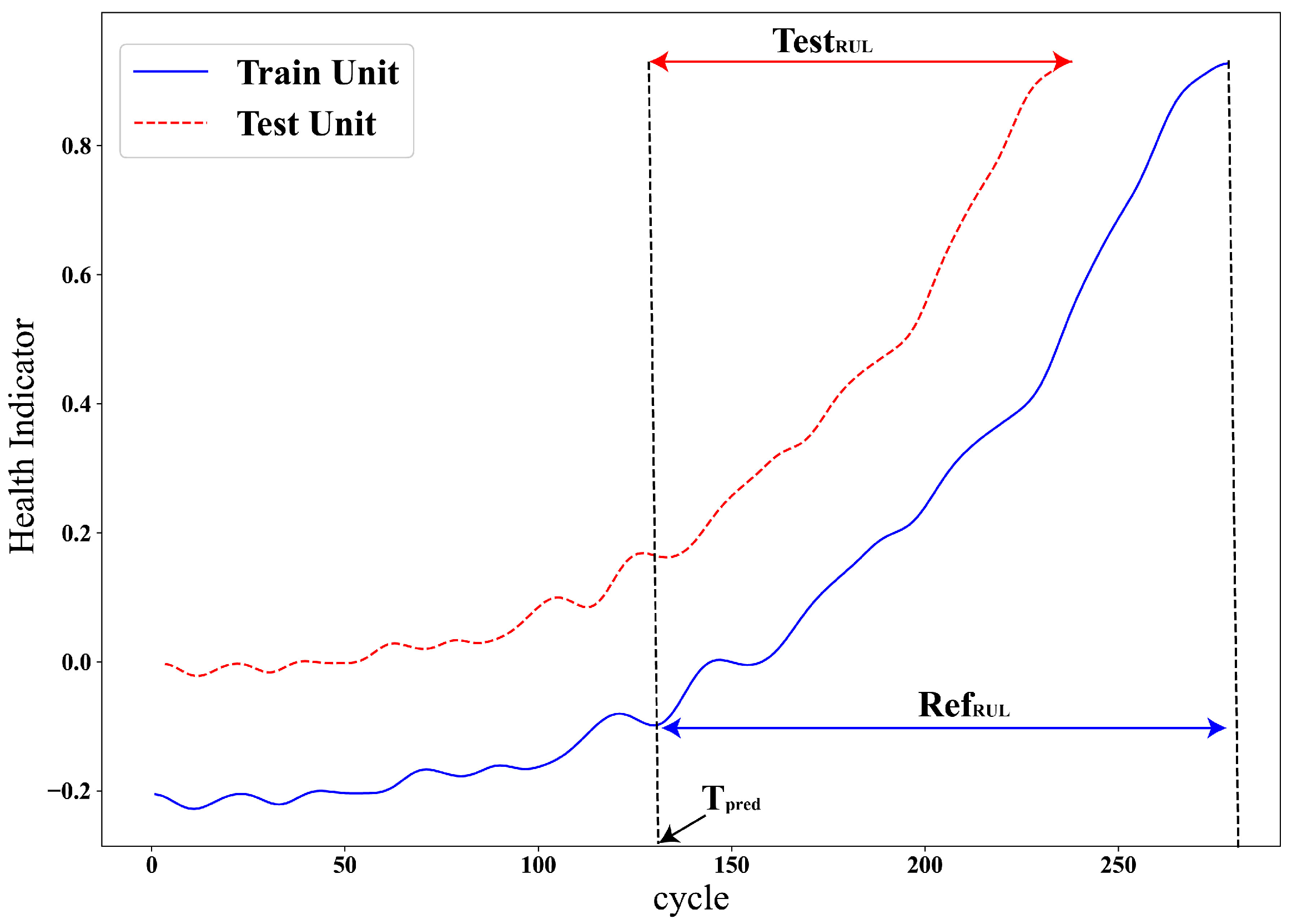
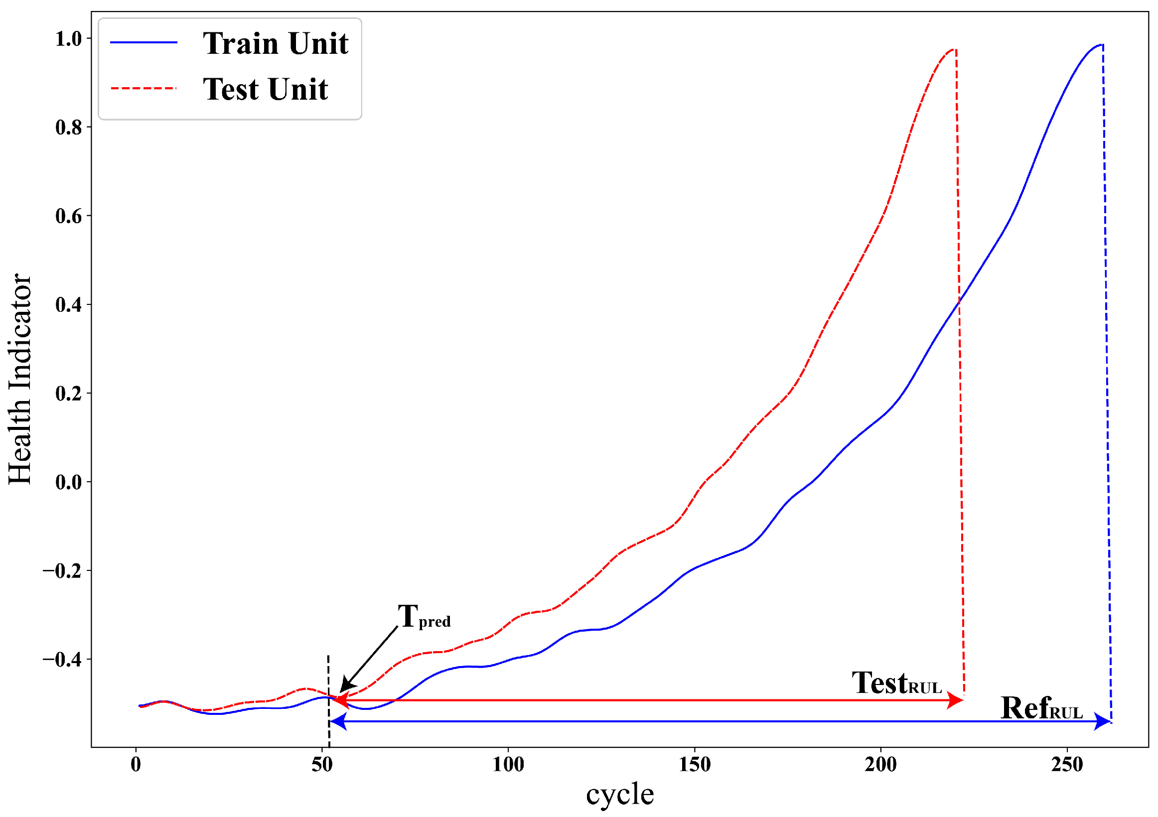
3.3.1. Reference RUL Adjustments

Using a reference system’s EOL directly for RUL estimation can lead to inaccuracies due to variations in initial wear and degradation rates.The initial wear of a system differs from one system to another, and in our experimental data, the initial wear was randomly selected. The degradation rate of different systems varies according to the different incidents. Moreover, in real-world scenarios, where each system is subjected to distinct operating conditions, loads, and environments, it is rare for two systems to possess identical degradation states from start to failure.
To address these challenges, we introduced the initial wear-based adjustment in Section 3.3.2 and the degradation rate-based adjustment in Section 3.3.3. These adjustments are implemented using a nonlinear sigmoid-like function, preventing excessive adjustment, as these functions yield an output within the [ 0 , 1 ] range. We fine-tuned these functions to produce an output within the [ 0.75 , 1.25 ] range to enhance the adjustment function’s effectiveness.
These functions ensure that if the test and reference systems have the same initial wear and degradation rates, the RUL of the reference system should not be adjusted. These sigmoid-like exponential adjustment functions are described as follows:
f ^ e x p ( x ) = 1 1 + e f ( x ) + 1 f ( α x ) , i f ( x 0 ) f ( β x ) , i f ( x < 0 )
Here, α and β are two scaling variables. α is applied to increase the reference RUL, whereas β decreases the reference RUL. A large value of the scaling variable results in a greater degree of change, whereas a small value results in a smaller degree. Therefore, this variable must be selected carefully; otherwise, under- or over-adjustment may occur. The evaluation of the selections of α and β is presented in Section 4. Later predictions are much worse than early predictions [2]. Thus, α is preferred to be relatively small in most applications.

3.3.2. Initial Wear Based Adjustment

The initial wear of the system is usually ignored in almost all similarity-based approaches. The selected RULs of the reference systems may not be directly applicable if their initial wear differs from the test system’s, as shown in Figure 7. A similar system has different initial wear, ending with a different RUL. The selected most similar reference and test systems may have the same degradation history but different initial wear. This difference also affects the RUL; for instance, a system with healthy initial wear tends to have a longer RUL, whereas a system with deteriorated initial wear usually has a shorter RUL. Therefore, adjusting the reference system’s RUL before estimating the test system’s RUL based on the initial conditions is more appropriate.
Given an HI of system S, its initial wear can be defined as
i n i t i a l W e a r = M e a n ( S 0 , S i ) ,
where we take the mean of the system from the start to i, where i is the index and its first 5 % of signal length. The initial wear difference between the test and the reference system is obtained by
I n i t i a l W e a r A d j u s t = i n i t i a l W e a r ( t e s t ) i n i t i a l W e a r ( r e f ) ,
the initial wear difference between the test system and its reference system can be obtained using Equation (9) and applied to adjust the reference RUL as
R U L r e f * = f ^ ( I n i t i a l W e a r A d j u s t ) × ( R U L r e f )
which is also present in Algorithm 1, line 11, where R U L r e f is the original reference RUL and R U L r e f * is the adjusted RUL. The reference RUL reduces if the test system start is healthier than the reference RUL, and vice versa.

3.3.3. Degradation Rate-Based Adjustment

The degradation rate is the most crucial indicator for RUL estimation. If the selected reference systems have different degradation rates than the test system, they may exhibit varying RULs, as shown in Figure 8. Systems with a steeper degradation rate are expected to fail earlier than those with smoother degradation rates. Hence, adjusting the RUL based on the differences in degradation rates is more suitable for this application. The degradation rate of a system can be calculated as follows:
D R a t e = M e a n ( X ( Δ n , n ) ) M e a n ( X ( i , Δ i ) ) n
We calculate degradation rates according to the test system’s length. For the test system, M e a n ( X ( Δ n , n ) ) represents the mean of the last few sample values from the test HI trajectory, and M e a n ( X ( i , Δ i ) ) signifies the mean of the initial values of the same system’s HI trajectory. In contrast, for a reference system, M e a n ( X ( Δ n , n ) ) denotes the mean of some middle values, equivalent to the length of the test trajectory from the reference HI trajectory, and M e a n ( X ( i , Δ i ) ) is the same as the mean of the test system.
The difference in the degradation rates between the test and reference systems was obtained using
R a t e B a e d A d j u s t = D R a t e ( t e s t ) D R a t e ( r e f )
The difference in the degradation rate was determined using Equation (12). This degradation-rate difference is then applied to modify the RUL of the chosen reference, rendering it more suitable, as follows:
R U L r e f * * = R a t e B a e d A d j u s t × ( R U L r e f * ) ,
which is also present in Algorithm 1, line 12, where R U L ref * represents the initially wear-based adjusted reference RUL, and R U L ref * * the rate-based adjusted RUL. The reference RUL decreases if the test system degrades more rapidly than the reference RUL and vice versa.

3.3.4. RUL Estimation

After applying the adjustments (initial wear-based adjustment in Section 3.3.2 and degradation rate-based adjustment in Section 3.3.3) to the selected reference RUL, the top k most similar adjusted reference RULs, denoted as R U L ref * * , are included for RUL estimation. Figure 9 illustrates CMAPSS dataset-I, system-55 in the red line, along with its top k = 10 most similar references selected for its RUL estimation (representing their EOL by *).
Since reference RULs may differ in relevance, a simple average could bias the final estimate. To mitigate this, we apply a weighted kernel density estimator, which emphasizes more representative reference systems. The weighted kernel density approximation for estimating the RUL of the test system can be expressed as follows:
r u l ^ = i = 1 k w i · K r u l r u l i h ,
where w i is the weight, K is a kernel function, and h is the bandwidth.
This procedure is also outlined in Algorithm 1 line 20. In this context, the kernel function is denoted as a non-negative function K, and h represents a smoothing parameter referred to as bandwidth in density estimation. Here, r u l i denotes the ith reference RUL in RUL \ , while K is a non-negative kernel function represented by K, and h is the smoothing parameter, also known as bandwidth in density estimation. Ultimately, the estimated r u l ^ obtained through the kernel density estimation function is considered the final estimate of the RUL for the test system.

4. Experimental Evaluation

This section showcases the effectiveness of the proposed DERUL framework. The datasets used for the evaluation, specifically the simulated turbofan engine degradation dataset C-MAPSS by NASA, are detailed in Section 4.1. The benchmark evaluation metrics are outlined in Section 4.3, which serves as a parameter for gauging effectiveness. Section 4.4 evaluates the proposed approach and compares it with other relevant state-of-the-art data-driven approaches to substantiate its efficacy.

4.1. Experimental Data

4.1.1. Aero Engine Degradation Dataset (C-MAPSS)

The experimental data employed to evaluate this framework is NASA’s publicly accessible C-MAPSS datasets, a standard benchmark for evaluating prognostics and health management algorithms [17,24,25]. The dataset was further divided into subsets operating under different operational and fault modes, as detailed in Table 1.
The train and test datasets were organized as [ n × 24 ] matrices, where n indicates the total number of data cycles, and 24 corresponds to different components. Each cycle encompasses 24 columns; the engine number is shown in the first column, the operational cycle number is specified in the second column, and the operational settings are encompassed in columns 3–5. Columns 6 to 24 represent 21 sensor values [17].
Multiple fault modes and diverse operating conditions enhance the realism of C-MAPSS engine degradation simulations, rendering it well suited for developing prognostics algorithms [26]. One can refer to [17] for further comprehensive information about the datasets.

4.1.2. Bearing Degradation Dataset (XJTU-SY)

The XJTU-SY dataset offers real-world bearing run-to-failure degradation data acquired from a controlled experimental setup [18]. It includes three distinct operating conditions, with five bearings tested under each condition. Vibration signals were captured along horizontal and vertical axes for every bearing.
In the data preprocessing phase, six time-domain statistical features were derived from each vibration channel: maximum amplitude, crest factor, root mean square, kurtosis, skewness, and variance. Consistent with the preprocessing strategy employed for the C-MAPSS dataset, the features were subjected to denoisation, normalization, and dimensionality reduction. PCA was utilized, and the first principal component accounting for 93% of the total variance was selected as the health degradation indicator. For this study, only the data from the first operating condition were considered. Unit 3 was chosen as the test set among the available bearings. The prediction target was defined as the RUL beginning from 70% of the total operational lifespan of the bearing up to the point of failure.

4.2. Data Normalization

Consistent with the comparative studies, we also normalized and noise reduction the data using
X = X X m i n X m a x X m i n
and
f ( x , σ ) = 1 2 π σ 2 exp 1 2 x σ 2

4.3. Evaluation Metrics

Experimental result evaluation aims to utilize metrics to assess whether the prognosis meets the task’s requirements. Consistent with most comparative studies [2,21,25,27,28,29], we also assess the model using an asymmetric MScore function (17) and RMSE (19). The definitions of these metrics are given by
S c o r e = e d i / 13 1 , d i > 0 , e d i / 10 1 , d i 0 ,
to be consistent with other studies, the mean of the score function is obtained as
M S c o r e = S c o r e t o t a l p r e d i c t i o n s ,
and
R M S E = 1 n i = 1 n d i 2 ,
to asses the accuracy of the framework.

4.4. Experimental Result

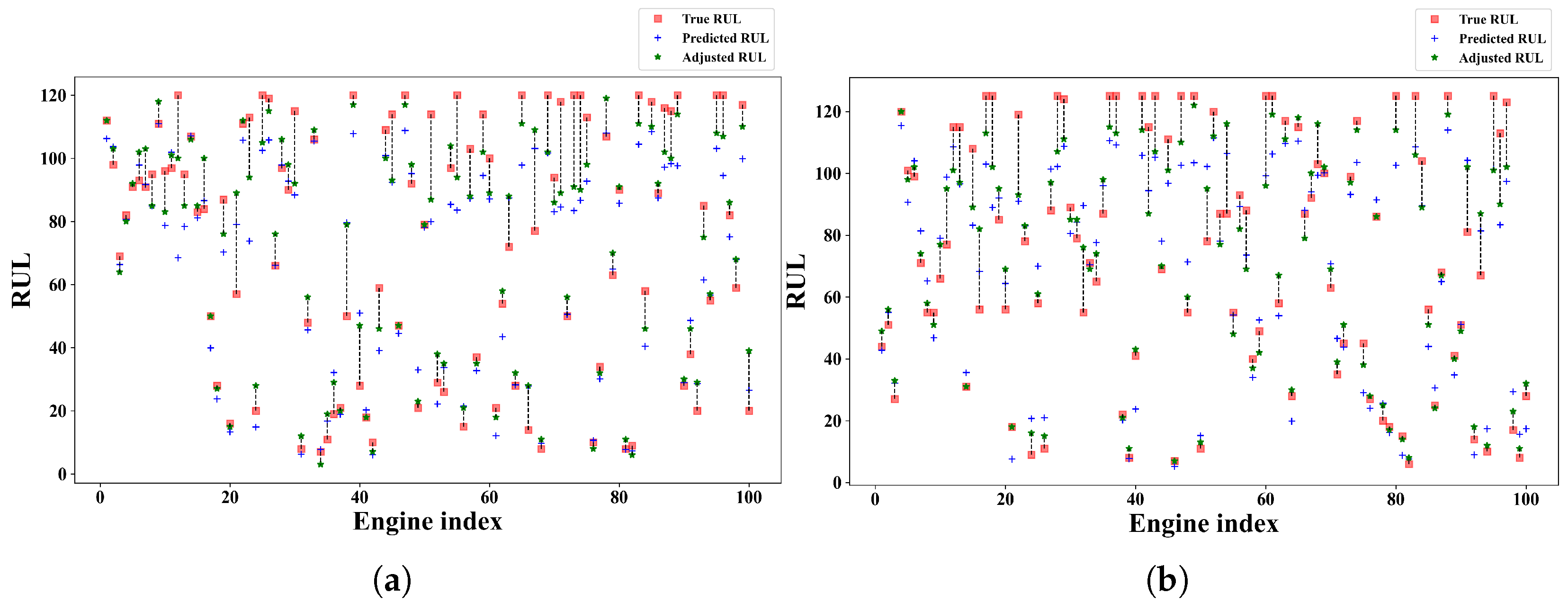
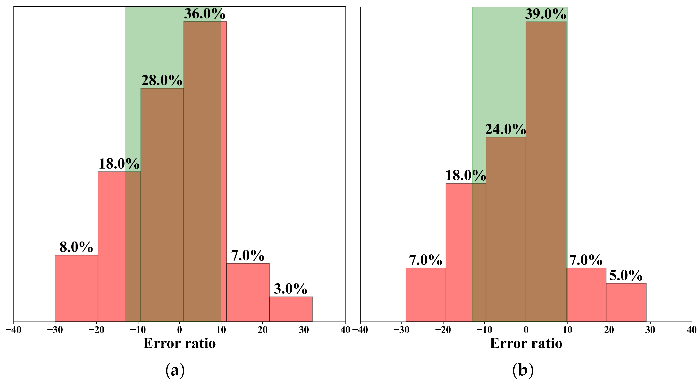
4.4.1. Experimentation on C-MAPSS

Figure 10 compares the final predicted RUL and actual RUL values for all engines across each subset. The red squares denote the actual RULs, predicted RUL using blue plus, and adjusted values by green stars. The vertical proximity between these symbols indicates the accuracy of the model’s prediction. Analysis of the results reveals that for datasets FD001 Figure 10a and FD003 Figure 10b, the majority of predicted values align closely with the actual values, exhibiting only minor discrepancies.
To evaluate the precision of DERUL’s estimation, Figure 11 presents a distribution of the RUL error ratio. The x-axis depicts the relative error ratio, while the y-axis represents the percentage of test instances for each error ratio about the total number of tests. The acceptable error ratio range, defined by the dataset creators’ scoring criteria, is indicated by a light green area (ranging from [−13 to 10]). The results demonstrate that for FD001 Figure 11a, the majority of predictions (68%) fall within the acceptable range, indicated by the green-shaded area, with a significant concentration (38%) centered around the zero error ratio. Similarly, for FD003 in Figure 11b, the majority of predictions (62%) fall within the acceptable range, indicated by the green-shaded area, with a significant concentration (35%) centered around the zero error ratio.
Comparison and discussion. This research conducts a comparative analysis of eight other models, encompassing both non-deep machine learning approaches and advanced deep learning models, as detailed in Table 2, where the best results are highlighted using bold font and the second-best results are distinguished by underlining. Similarity-based approaches have seen significant advancements in frameworks for RUL estimation. Among these, ref. [2] developed the multi-local similarity-based RUL estimation framework. Ref. [30] proposed the Enhanced Adaptive Guided Differential Evolution (EAGDE) algorithm to optimize Support Vector Machine (SVM) parameters, thereby improving prediction accuracy. Additionally, ref. [31] introduced the spherical-DTW method, which addresses challenges in nonlinearity during distance measurement across different degradation stages and aligns degradation patterns with temporal variations.
To assess the computational efficiency of our method, we compared the average inference time per test instance against a baseline multi-local similarity-based approach that utilizes the complete time series without DE extraction. Experiments conducted on FD001 and FD003 datasets show that our DE-based method achieves a runtime reduction of approximately 14.39% and 17.26%, confirming its potential for real-time deployment.
The proposed model demonstrates significant improvements over baseline studies in RUL estimation, as outlined in Table 2. Compared with the base model [2], it achieves a 12.33% reduction in RMSE and an 18.93% increase in prognostic m-score, indicating enhanced predictive accuracy and reliability. Compared with similar non-deep machine learning methods, it outperforms all existing studies, showcasing its robustness in capturing degradation patterns.
Recent deep learning and similarity-based RUL estimation frameworks often require significant training data and high computational costs. Our approach mitigates these issues by leveraging DEs, necessitating less training data, and offering more straightforward hyperparameter tuning. Additionally, the method is computationally efficient, making it viable for real-time industrial applications. This efficiency stems from its ability to capture and effectively utilize degradation patterns compared with traditional methods. The proposed model’s performance is compared with several state-of-the-art similarity-based and recent deep-learning models for RUL estimation.

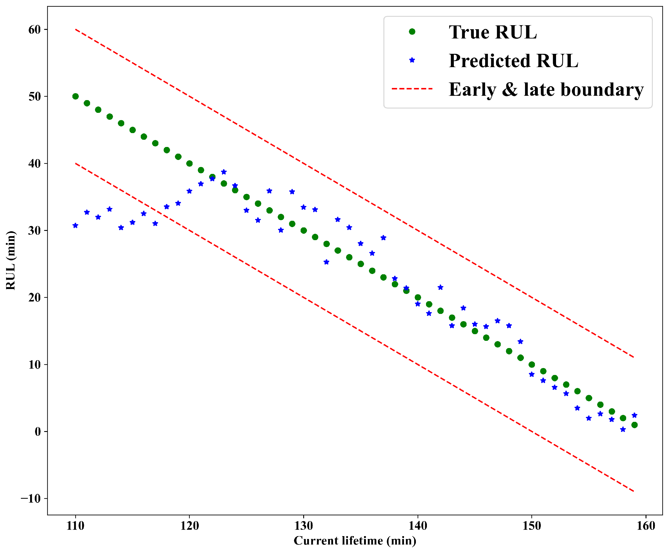
4.4.2. Experimentation on XJTU-SY

The predicted RULs for the bearings are presented in Figure 12. Initially, the predicted RULs exhibit minor deviations from the ground truth; however, they converge closely to the actual RULs as the bearing approaches failure. Among the predictions, 84.3% were accurate, 15.7% were early, and none were late.
In addition, the prediction performance of four similarity-based approaches was evaluated on the XJTU-SY dataset: a global similarity-based method, a local similarity-based method, our proposed multi-local similarity method without degradation rate-based adjustment, and the same method with the adjustment. The comparative results are summarized in Table 3.
Our method—both with and without the adjustment—consistently outperforms the baseline similarity-based approaches. Specifically, when the degradation rate-based adjustment is incorporated, the RMSE is reduced by 9.40% and 6.57% compared with the best-performing similarity-based method. The local similarity-based approach yields the poorest performance. This is attributed to its tendency to match reference trajectories based on overall distance, thereby overlooking the critical influence of recent state information, which is often more predictive of imminent degradation. While the local similarity-based method performs better, its accuracy remains constrained due to its disregard for historical state dynamics.

4.5. Further Analysis
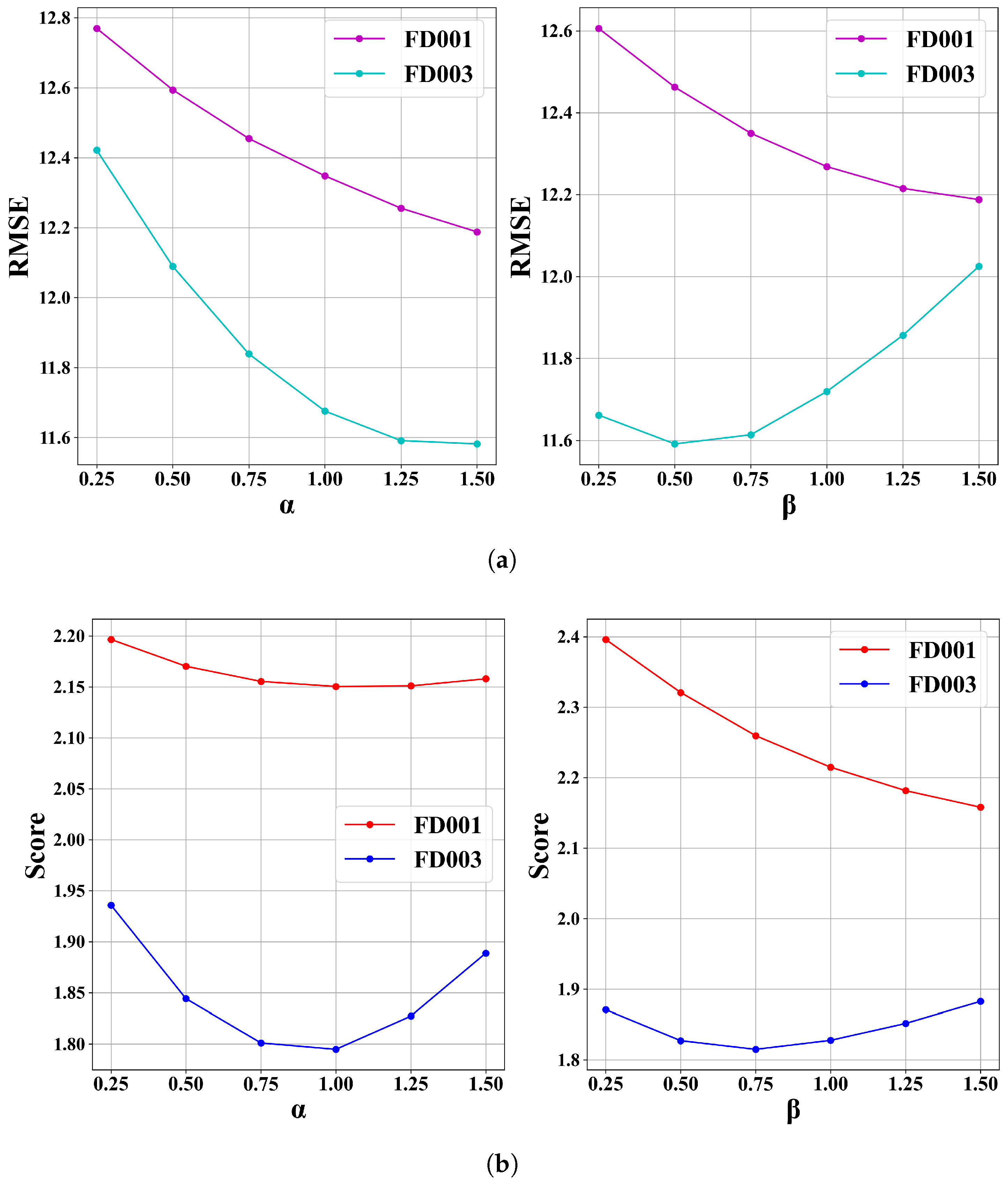
In this section, we further analyze the performance of the proposed method using FD001 of C-MAPSS.

4.5.1. Impact of Adjustment Parameters α and β

To assess the sensitivity of the proposed method to the adjustment parameters α and β used in the reference RUL adjustment process, we conducted a grid search over a predefined range of values: {[0.25, 0.5, 0.75, 1.0, 1.25, 1.5]}. The evaluation was performed on FD001 and FD003 datasets using score and RMSE as performance metrics.
Figure 13 shows the effects of varying α and β . As can be observed, both parameters influence model performance nonlinearly. For α , the optimal values of the lowest score and RMSE are found around α = 1.0 for both datasets, with marginal improvements tapering off beyond this point. Similarly, β = 1.5 yields the best RMSE on FD001 and close-to-optimal performance on FD003.
These results indicate that while performance is moderately sensitive to these parameters, the model remains relatively stable across a broad range, suggesting robustness. To ensure a fair comparison, the optimal parameters were used for each dataset in the experiments reported in Section 4.

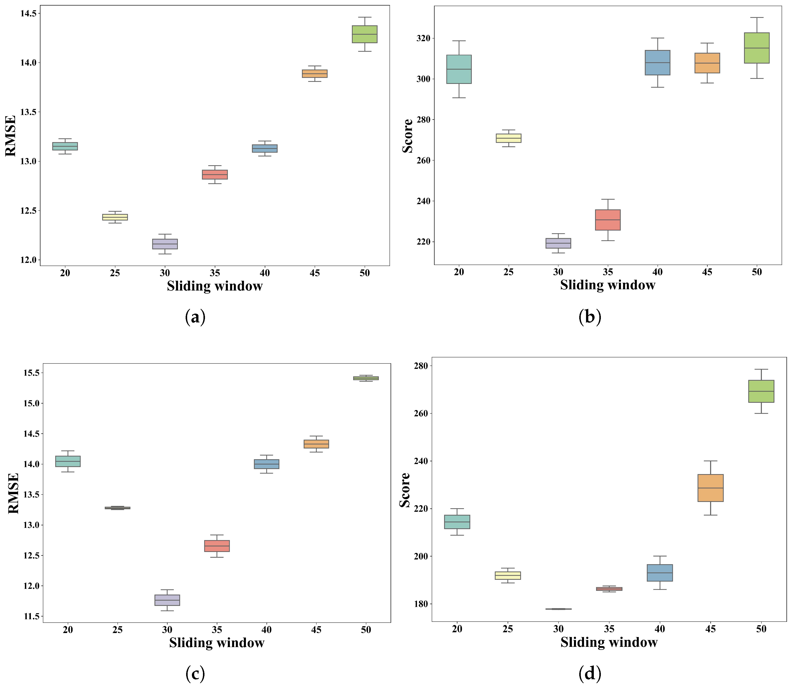
4.5.2. Effect of the Window Size

To evaluate the impact of sliding window size, we conducted across a range of window sizes (20, 25, …, 50). The corresponding prediction performance, measured by Root Mean Square Error (RMSE) and the evaluation score, is presented in Figure 14. The experiment reveals a better performance at a window size of 30, which achieves the lowest RMSE and score, indicating optimal temporal representation for degradation pattern learning.
Notably, smaller window sizes tend to under-perform, likely due to insufficient historical context, while larger windows degrade performance by incorporating excessive or less relevant past information. These results emphasize the importance of selecting an appropriate window size to balance short-term sensitivity with long-term trend awareness in time-series degradation modeling.

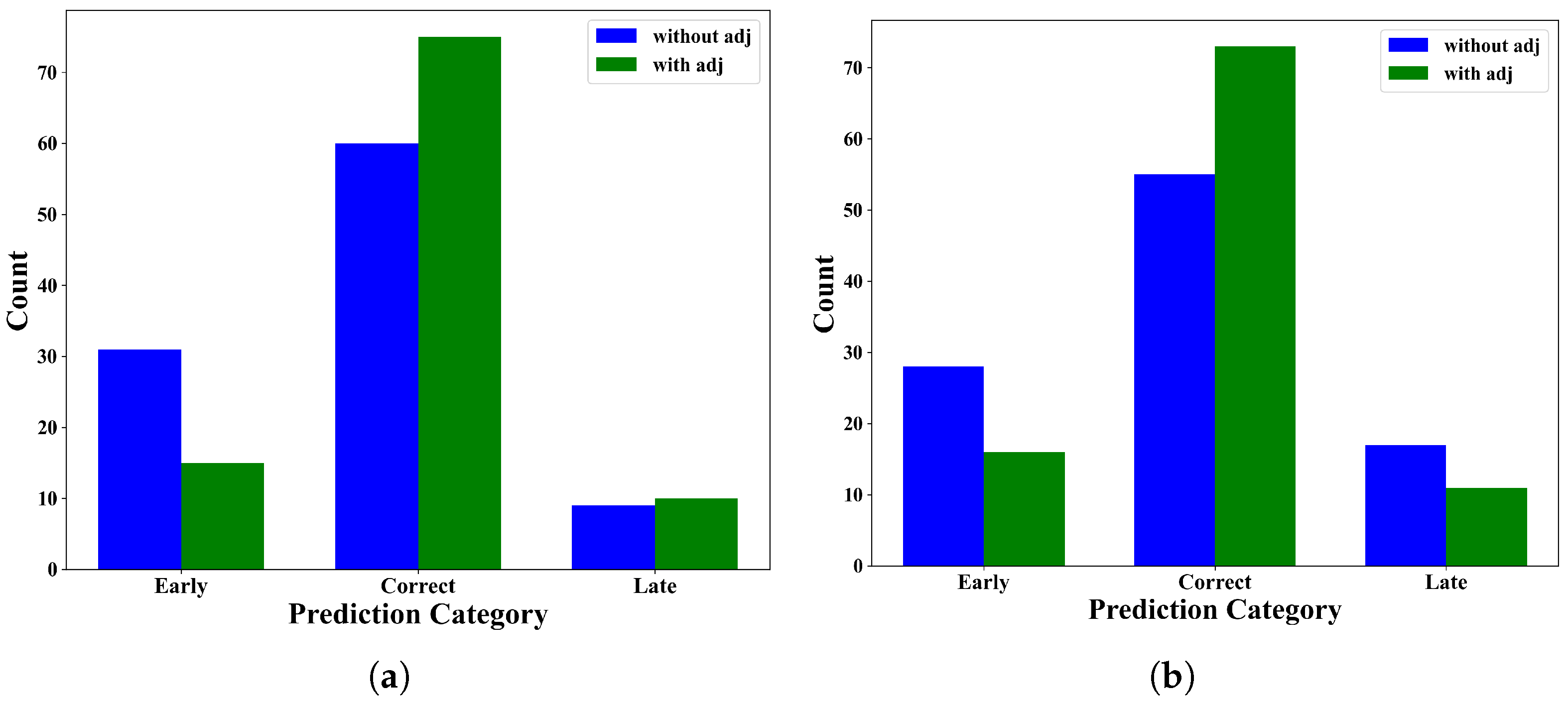
4.5.3. Effect of Adjustment Strategies

Figure 15 illustrates the impact of the proposed adjustment strategies on the estimation accuracy. The diagram compares the number of correct, early, and late predictions with and without adjustment strategies. The results demonstrate a notable increase in the proportion of accurate predictions, indicating improved alignment between the predicted and actual RUL values. Simultaneously, the adjustment strategies effectively reduce early and late predictions, highlighting the model’s enhanced capability to capture the actual degradation patterns. This improvement reflects the proposed initial wear-based adjustment and degradation rate-based adjustment strategies positively impact the model’s ability, reducing prediction bias and enhancing overall reliability in RUL estimation.

5. Conclusions and Future Work

This study has introduced a novel RUL estimation framework predicated on identifying and utilizing degradation events (DEs) within system operational trajectories. Departing from conventional approaches that rely on complete historical trajectories or terminal operational states, the proposed methodology demonstrates that strategically selected subsequences exhibiting significant degradation characteristics serve as more reliable indicators for prognostic modeling. Extracting these degradation events enables a targeted selection of reference systems while implementing two distinct adjustment strategies—initial wear compensation and degradation rate normalization—to address inherent variabilities in operational baselines and deterioration trajectories.
Experimental validation was conducted across benchmark and real-world operational datasets, including the C-MAPSS turbofan engine and XJTU-SY bearing degradation data. The results substantiate the framework’s superior performance relative to contemporary state-of-the-art models while simultaneously achieving computational efficiency gains of approximately 30% in inference latency.
Notwithstanding these advancements, certain limitations warrant acknowledgment and present opportunities for further investigation. While effective for single-mode operational conditions, the current implementation would benefit from enhanced capability to accommodate systems exhibiting multiple operational modes or complex nonlinear degradation patterns. Future research will focus on three principal areas: integrating advanced temporal alignment methodologies, incorporating deep learning architectures to model intricate fault progression, and extensive validation across broader industrial applications to establish universal applicability. These extensions address current constraints while advancing the framework toward deployment in practical prognostic systems across diverse industrial domains.

Author Contributions

Z.A.: conceptualization, methodology, software, writing—original draft, writing—review and editing. M.S.: writing—review and editing. M.H. (Musrat Hussain): writing—review and editing, funding. N.H.: writing—review and editing. M.H. (Mehboob Hussain): writing—review and editing, correspondence, funding. N.A.K.: writing—review and editing, supervision. All authors have read and agreed to the published version of the manuscript.

Funding

Funding for this work is provided by the Fundamental Research Funds for the Central Universities under Grant No. 2682024CX018.

Institutional Review Board Statement

Not applicable.

Informed Consent Statement

Not applicable.

Data Availability Statement

The dataset is publicly available at https://ti.arc.nasa.gov/tech/dash/groups/pcoe/prognostic-data-repository/(accessed on 15 December 2023).

Conflicts of Interest

The authors declare no conflicts of interest.

References

  1. Yang, B.; Liu, R.; Zio, E. Remaining useful life prediction based on a double-convolutional neural network architecture. IEEE Trans. Ind. Electron. 2019, 66, 9521–9530. [Google Scholar] [CrossRef]
  2. Lyu, J.; Ying, R.; Lu, N.; Zhang, B. Engineering Applications of Artificial Intelligence Remaining useful life estimation with multiple local similarities. Eng. Appl. Artif. Intell. 2020, 95, 103849. [Google Scholar] [CrossRef]
  3. Calabrese, M.; Cimmino, M.; Fiume, F.; Manfrin, M.; Romeo, L.; Ceccacci, S.; Paolanti, M.; Toscano, G.; Ciandrini, G.; Carrotta, A.; et al. SOPHIA: An Event-Based IoT and Machine Learning Architecture for Predictive Maintenance in Industry 4.0. Information 2020, 11, 202. [Google Scholar] [CrossRef]
  4. Hu, Q.; Zhao, Y.; Wang, Y.; Peng, P.; Ren, L. Remaining Useful Life Estimation in Prognostics Using Deep Reinforcement Learning. IEEE Access 2023, 11, 32919–32934. [Google Scholar] [CrossRef]
  5. Solís-Martín, D.; Galán-Páez, J.; Borrego-Díaz, J. On the Soundness of XAI in Prognostics and Health Management (PHM). Information 2023, 14, 256. [Google Scholar] [CrossRef]
  6. Arunan, A.; Qin, Y.; Li, X.; Yuen, C. A change point detection integrated remaining useful life estimation model under variable operating conditions. Control Eng. Pract. 2024, 144. [Google Scholar] [CrossRef]
  7. Behera, S.; Patel, Y.S.; Choubey, A.; Misra, R.; Kanani, C.S.; Sillitti, A. Ensemble trees learning based improved predictive maintenance using IIoT for turbofan engines. In Proceedings of the 34th ACM Symposium on Applied Computing, New York, NY, USA, 8–12 April 2019; pp. 842–850. [Google Scholar] [CrossRef]
  8. Xu, F.; Yang, F.; Fan, X.; Huang, Z.; Tsui, K.L. Extracting degradation trends for roller bearings by using a moving-average stacked auto-encoder and a novel exponential function. Measurement 2020, 152, 107371. [Google Scholar] [CrossRef]
  9. Liang, Z.; Gao, J.; Jiang, H.; Gao, X.; Gao, Z.; Wang, R. A Degradation Degree Considered Method for Remaining Useful Life Prediction Based on Similarity. Comput. Sci. Eng. 2019, 21, 50–64. [Google Scholar] [CrossRef]
  10. Roberto De Oliveira Da Costa, P.; Akcay, A.; Zhang, Y.; Kaymak, U.; de Oliveira da Costa, P.R.; Akcay, A.; Zhang, Y.; Kaymak, U. Attention and Long Short-Term Memory Network for Remaining Useful Lifetime Predictions of Turbofan Engine Degradation. Int. J. Progn. Health Manag. 2019, 10, 034. [Google Scholar]
  11. Haque, M.S.; Choi, S.; Baek, J. Auxiliary particle filtering-based estimation of remaining useful life of IGBT. IEEE Trans. Ind. Electron. 2018, 65, 2693–2703. [Google Scholar] [CrossRef]
  12. Li, N.; Lei, Y.; Yan, T.; Li, N.; Han, T. A wiener-process-model-based method for remaining useful life prediction considering unit-to-unit variability. IEEE Trans. Ind. Electron. 2019, 66, 2092–2101. [Google Scholar] [CrossRef]
  13. Huang, C.G.; Huang, H.Z.; Li, Y.F. A Bidirectional LSTM Prognostics Method Under Multiple Operational Conditions. IEEE Trans. Ind. Electron. 2019, 66, 8792–8802. [Google Scholar] [CrossRef]
  14. Liu, K.; Hu, X.; Wei, Z.; Li, Y.; Jiang, Y. Modified Gaussian Process Regression Models for Cyclic Capacity Prediction of Lithium-Ion Batteries. IEEE Trans. Transp. Electrif. 2019, 5, 1225–1236. [Google Scholar] [CrossRef]
  15. Ma, M.; Sun, C.; Mao, Z.; Chen, X. Ensemble deep learning with multi-objective optimization for prognosis of rotating machinery. ISA Trans. 2021, 113, 166–174. [Google Scholar] [CrossRef] [PubMed]
  16. Bektas, O.; Jones, J.A.; Sankararaman, S.; Roychoudhury, I.; Goebel, K. A neural network framework for similarity-based prognostics. MethodsX 2019, 6, 383–390. [Google Scholar] [CrossRef] [PubMed]
  17. Saxena, A.; Goebel, K.; Simon, D.; Eklund, N. Damage propagation modeling for aircraft engine run-to-failure simulation. In Proceedings of the 2008 International Conference on Prognostics and Health Management, PHM 2008, Denver, CO, USA, 6–9 October 2008; pp. 11–19. [Google Scholar] [CrossRef]
  18. Wang, B.; Lei, Y.; Li, N.; Li, N. A Hybrid Prognostics Approach for Estimating Remaining Useful Life of Rolling Element Bearings. IEEE Trans. Reliab. 2020, 69, 401–412. [Google Scholar] [CrossRef]
  19. Huang, C.G.; Huang, H.Z.; Peng, W.; Huang, T. Improved trajectory similarity-based approach for turbofan engine prognostics. Mech. Syst. Signal Process. 2019, 33, 4877–4890. [Google Scholar] [CrossRef]
  20. Ren, Y.; Lyu, J.; Jebali, M.; Zhang, B. An AC Contactor Remaining Useful Life Prediction Method based on Degradation Event Analysis. In Proceedings of the 2023 6th International Symposium on Autonomous Systems (ISAS), Nanjing, China, 23–25 June 2023; pp. 1–6. [Google Scholar]
  21. Aydemir, G.; Acar, B. Anomaly monitoring improves remaining useful life estimation of industrial machinery. J. Manuf. Syst. 2020, 56, 463–469. [Google Scholar] [CrossRef]
  22. Kumar, P.S.; Kumaraswamidhas, L.A.; Laha, S.K.; Shankar, P.; Kumaraswamidhas, L.A.; Laha, S.K. Selection of efficient degradation features for rolling element bearing prognosis using Gaussian Process Regression method. ISA Trans. 2021, 112, 386–401. [Google Scholar] [CrossRef]
  23. Biggio, L.; Kastanis, I. Prognostics and Health Management of Industrial Assets: Current Progress and Road Ahead. Front. Artif. Intell. 2020, 3, 578613. [Google Scholar] [CrossRef]
  24. Bektas, O.; Jones, J.A.; Sankararaman, S.; Roychoudhury, I.; Goebel, K. A neural network filtering approach for similarity-based remaining useful life estimation. Int. J. Adv. Manuf. Technol. 2019, 101, 87–103. [Google Scholar] [CrossRef]
  25. Chen, Z.; Wu, M.; Zhao, R.; Guretno, F.; Yan, R.; Li, X. Machine Remaining Useful Life Prediction via an Attention-Based Deep Learning Approach. IEEE Trans. Ind. Electron. 2021, 68, 2521–2531. [Google Scholar] [CrossRef]
  26. Ramasso, E. Investigating computational geometry for failure prognostics. Int. J. Progn. Health Manag. 2014, 5, 1–18. [Google Scholar] [CrossRef]
  27. Kang, Z.; Catal, C.; Tekinerdogan, B. Remaining useful life (Rul) prediction of equipment in production lines using artificial neural networks. Sensors 2021, 21, 932. [Google Scholar] [CrossRef]
  28. Fan, L.; Chai, Y.; Chen, X. Trend attention fully convolutional network for remaining useful life estimation. Reliab. Eng. Syst. Saf. 2022, 225, 108590. [Google Scholar] [CrossRef]
  29. Sternharz, G.; Elhalwagy, A.; Kalganova, T. Data-Efficient Estimation of Remaining Useful Life for Machinery With a Limited Number of Run-to-Failure Training Sequences. IEEE Access 2022, 10, 129443–129464. [Google Scholar] [CrossRef]
  30. Abdelghafar, S.; Khater, A.; Wagdy, A.; Darwish, A.; Hassanien, A.E. Aero engines remaining useful life prediction based on enhanced adaptive guided differential evolution. Evol. Intell. 2024, 17, 1209–1220. [Google Scholar] [CrossRef]
  31. Li, X.; Xu, S.; Yang, Y.; Lin, T.; Mba, D.; Li, C. Spherical-dynamic time warping—A new method for similarity-based remaining useful life prediction. Expert Syst. Appl. 2024, 238. [Google Scholar] [CrossRef]
  32. Wen, Z.; Fang, Y.; Wei, P.; Liu, F.; Chen, Z.; Member, S.; Wu, M. Temporal and heterogeneous graph neural network for remaining useful life prediction. arXiv 2024, arXiv:2405.04336. [Google Scholar]
Figure 1. Comparison of local similarity-based and DE-based mechanisms for a sequence experiencing a DE. (a) An approach based on local similarities necessitates comparing “n” local segments of the test system with corresponding segments from the training system. (b) A DE-based approach focuses on comparing only the top “k” local segments with the highest disparity in the test system against all segments of the training system. The red * denote the “k” local segments exhibiting the highest disparity, highlighting potential degradation events.
Information 16 00542 g001
Figure 2. Proposed framework dataflow diagram.
Information 16 00542 g002
Figure 3. Distance profile D P of T ( i , m ) and T. The lowest points from D P correspond to the querying subsequence T ( i , m ) . The gray area region represents the exclusion zone.
Information 16 00542 g003
Figure 4. The difference between the distance profile D P and the matrix profile M P .
Information 16 00542 g004
Figure 5. The top section of the figure depicts the HI, and the bottom section shows the matrix profile, with a red (*) indicating the potential DE’s of the system.
Information 16 00542 g005
Figure 6. Health indicator (a) and matrix profile (b) representing the most similar DE.
Information 16 00542 g006
Figure 7. Initial wear difference between different systems.
Information 16 00542 g007
Figure 8. Degradation rate differences of test between test and reference systems.
Information 16 00542 g008
Figure 9. The blue lines represent all available reference HIs, while the blue HIs with x black cross represent the selected most similar adjusted RULs.
Information 16 00542 g009
Figure 10. RUL prediction and ground truth values for FD001 (a) and FD003 (b).
Information 16 00542 g010
Figure 11. The relative frequency distribution of RUL prediction error ratios for FD001 (a) and FD003 (b).
Information 16 00542 g011
Figure 12. Prediction result of the proposed framework using XJTU-SY.
Information 16 00542 g012
Figure 13. Grid search results for different values of α and β on FD001 and FD003 using RMSE (a) and score (b).
Information 16 00542 g013
Figure 14. Effect of sliding window size on RMSE (a), and Score (b) using FD001, and RMSE (c) and score (d) using FD003.
Information 16 00542 g014
Figure 15. Comparison of prediction categories With and without adjustment for FD001 (a) and FD003 (b).
Information 16 00542 g015
Table 1. Dataset description.
DatasetsOperating ConditionsFault ModesTraining DatasetTest DatasetRUL Dataset
DimensionDimensionDimension
FD0011120,631 × 2413,096 × 24100
FD0026153,759 × 2433,991 × 24259
FD0031224,720 × 2416,596 × 24100
FD0046261,249 × 2441,214 × 24248
Table 2. Prediction performance comparison on the CMAPSS dataset (RMSE, lower is better).
Models/DatasetsYearFD001FD003
RMSEM-ScoreRMSEMScore
Deep learning based models
Anomaly-Triggered-RUL [21]202017.1539217.6520
LSTM-Transformer [25]202114.53322--
TaFCN [28]202213.9933612.01251
Changepoint LSTM [6]202413.5922412.94207
THGNN [32]202413.1528512.61255
Machine learning (non-deep)-based models
Multi-Local Similarities [2]202014.126415.36271
EAGDE–SVM [30]202214.1025318.86514
Spherical-DTW [31]202426.19---
RUL-DE (Without Adj)202514.5326913.15231
RUL-DE (Proposed)202512.3321411.59178
Boldface represents the best-performing and underline represents the second best-performing framework on the selected dataset.
Table 3. Performance comparison of four different similarity-based methods.
Method (Similarity-Based)RMSEMScore
Local9.881.29
Multi-local similarities8.400.76
RUL-DE (without adj)8.170.75
RUL-DE (proposed)7.610.71
Disclaimer/Publisher’s Note: The statements, opinions and data contained in all publications are solely those of the individual author(s) and contributor(s) and not of MDPI and/or the editor(s). MDPI and/or the editor(s) disclaim responsibility for any injury to people or property resulting from any ideas, methods, instructions or products referred to in the content.

