Intelligent Teaching Recommendation Model for Practical Discussion Course of Higher Education Based on Naive Bayes Machine Learning and Improved k-NN Data Mining Algorithm

Abstract

Aiming at the existing problems in practical teaching in higher education, we construct an intelligent teaching recommendation model for a higher education practical discussion course based on naive Bayes machine learning and an improved k-NN data mining algorithm. Firstly, we establish the naive Bayes machine learning algorithm to achieve accurate classification of the students in the class and then implement student grouping based on this accurate classification. Then, relying on the student grouping, we use the matching features between the students’ interest vector and the practical topic vector to construct an intelligent teaching recommendation model based on an improved k-NN data mining algorithm, in which the optimal complete binary encoding tree for the discussion topic is modeled. Based on the encoding tree model, an improved k-NN algorithm recommendation model is established to match the student group interests and recommend discussion topics. The experimental results prove that our proposed recommendation algorithm (PRA) can accurately recommend discussion topics for different student groups, match the interests of each group to the greatest extent, and improve the students’ enthusiasm for participating in practical discussions. As for the control groups of the user-based collaborative filtering recommendation algorithm (UCFA) and the item-based collaborative filtering recommendation algorithm (ICFA), under the experimental conditions of the single dataset and multiple datasets, the PRA has higher accuracy, recall rate, precision, and F1 value than the UCFA and ICFA and has better recommendation performance and robustness.

1. Introduction

The goal of higher education is to cultivate innovative and applied talents [1]. It focuses on cultivating students’ interests and improving their practical abilities, encouraging students to transform their theoretical knowledge into practical skills [2]. Based on the training objectives of higher education, course design includes two parts: theoretical teaching and practical teaching [3]. Practical teaching focuses on cultivating and examining the students’ mastery of a certain skill [4]. Traditionally, the basic teaching mode of practical courses is “teacher transferring knowledge”, which means that the teachers design the teaching content while the students passively receive it [5]. The process of this teaching mode is relatively simple. The teachers firstly determine and analyze the theoretical course content, and then extract the skills and requirements involved in the course, determine the practical content based on the skills and requirements, and divide the practical content into several implementation steps, which will be completed by the student groups. At the end of the course, the entire practical teaching activity is summarized by the whole class [6]. This process mainly involves three steps: firstly, the design of the practical content; secondly, grouping students based on the practical topics; and thirdly, the implementation of the practical teaching [7]. Analyzing the design and implementation process of practical teaching in the traditional mode, it can be concluded that the teachers play a leading role in this process. The design of the practical topics, the student grouping, and the implementation and evaluation of practical teaching are all independently completed by the teachers. Students participate in the entire practical course, receive the practical content designed by the teachers, and complete the practical content [8]. This mode has the features of teacher control, prominent theme, and strong pertinence. It can effectively explore the core content of the theoretical course, transform the theoretical teaching content into practical content, guide students to complete the practice in order, and improve the students’ skills in a targeted manner [9].

In addition, there are some other commonly used teaching methods in practical courses, such as the scenario simulation method, the experimental operation method, the task-driven method, the game teaching method, the visiting teaching method, and so on. In the scenario simulation method, the teachers design the teaching scenarios, and the students are divided into groups to perform, identify, and solve problems [10]. In the experimental operation method, the teachers design the experimental content and process, and the students are divided into groups to complete the experiment. Students are required to perform hands-on operations to discover and solve problems during the experimental process [11]. In the task-driven method, the teachers design specific tasks, the students are divided into groups, and the teachers ask each group to complete different tasks to achieve the specified goals [12]. In the game teaching method, the teachers design games with simulated scenarios, in which the students are grouped together to participate and solve problems during the game process [13]. In the visiting teaching method, the teachers lead the students to visit the teaching site, in which the students are divided into groups to discuss and solve problems [14]. These practical teaching methods have their own features, but they all rely on three aspects: the teaching content design, the student grouping, and the practical teaching implementation. Based on the teaching objectives and contents, the three core elements of practical teaching are analyzed, and the following problems in the traditional practical teaching mode are summarized.

The design of practical content is based on the teachers’ teaching experience and their mastery of the teaching content. The practical topics are determined by their qualitative description. This approach lacks a quantitative method for practical topics, and there is no clear quantitative method to explore and visualize the core elements involved in the teaching content. Meanwhile, the design of the practical content lacks a quantitative standard and executable method to guide the teachers in exploring the practical elements, resulting in low accuracy in the design of practical topics.

Grouping students is based on the teachers’ experience and the students’ free matching, without strict grouping criteria or a scientifically quantified grouping method. The grouping process is highly random and casual, and the features and interests of group members vary greatly, resulting in low accuracy of grouping.

The implementation of the practical teaching lacks personalized interest mining or a method for matching and recommending practical content based on the interest mining results, resulting in a low degree of matching between the practical topics and the interests of each group’s members. This ultimately leads to a low quality of practical teaching and poor classroom teaching effectiveness.

In response to the above problems, the practical teaching mode needs to be optimized from three aspects: quantitative modeling of the core elements of the practical topics, a quantitative grouping algorithm model for the students, and a matching and recommendation algorithm model for the practical topics [15]. Firstly, it is necessary to determine the practical teaching topics based on the theoretical teaching content, explore the core element labels of the practical teaching topics, and construct a label quantification model. Secondly, based on the label quantification model, the student interest mining model and the algorithm model for the student grouping are constructed to achieve accurate classifications of students, so that students within the same group all have the closest interests. We establish a practical topic recommendation algorithm based on the student grouping model, with interest mining and matching as the core methods. It aims to accurately recommend the practical topics for each group; then, the teachers and students make decisions based on the recommendation results [16]. According to the problem analysis and the modeling principle, we construct an intelligent teaching recommendation model for a higher education practical discussion course based on naive Bayes machine learning and an improved k-NN data mining algorithm. The main work includes the following aspects.

(1)

We analyze the research background of “artificial intelligence plus education” and the current status and existing problems of practical teaching methods. In response to these problems, we propose the advantages of the intelligent teaching recommendation model based on naive Bayes machine learning and improved k-NN data mining algorithm.

(2)

We construct the student grouping algorithm based on naive Bayes machine learning. Firstly, we establish the training set model for the naive Bayes machine learning algorithm and collect the training dataset from the previous classes. Secondly, we set up a naive Bayes machine learning model to group the students in a class, so that each group of students has the closest interests.

(3)

We build a teaching recommendation model based on the improved k-NN data mining algorithm by implementing the class grouping. Firstly, an optimal complete binary encoding tree for the discussion topic is constructed, and the feature attributes of the discussion topic are matched based on the interests of each group of students. The binary encoding tree is established based on the spatial coordinate system of the discussion topic, and the recommendation model is established on the coordinate system.

(4)

We design the experiments to validate the proposed algorithm, demonstrating its feasibility from three aspects as detailed in the following sections: “Results and Analysis on the Naive Bayes Grouping”, “Results and Analysis on the Proposed Teaching Recommendation Algorithm”, and “Results and Analysis of the Comparative Experiment”. Compared with the traditional collaborative filtering algorithms, the proposed algorithm has higher accuracy, recall rate, precision, and F1 value.

2. Related Works and the Advantages, Application Purpose, Formulated Requirements, and Constraints of the Proposed Model

2.1. Related Works

In the field of artificial intelligence development, the integration of intelligent algorithms into teaching practice is currently a hot research topic. The research on teaching recommendation algorithms mainly focuses on the combination of recommendation algorithms with teaching platform development, teaching design, teaching evaluation, and other aspects. Ren [17] constructed an e-learning-based recommendation model incorporating the user’s previous behaviors, which are used to mine the user’s interest data and recommend Chinese learning resources. The model has been experimentally tested and shows good performance. Fu et al. [18] designed a multimedia system based on Chinese language teaching by combining data mining techniques and recommendation algorithms. The research optimized and improved the information resource library of the system from the perspective of users and added system functions to meet the personalized needs of certain users. It enhances the efficiency of the teaching system. Yin [19] developed an improved collaborative filtering algorithm that combined users’ social relationships and behavioral characteristics to recommend relevant teaching content for music teaching platforms. The algorithm applies the users’ social relationships to construct the similarity calculation formula and uses the behavioral feature data as the basis for recommendation calculation, improving the accuracy of the recommendation algorithm. Liu [20] established a new mode of college English teaching based on the personalized recommendation of teaching resources and developed a teaching recommendation model based on a collaborative filtering algorithm to improve the accuracy of the recommendation algorithm. Zhang et al. [21] established a recommendation model for the online teaching of Chinese as a foreign language based on user interest similarity using a collaborative filtering recommendation algorithm. Three experiments were designed to prove that the constructed algorithm has good recommendation performance. Ying [22] developed an interactive AI virtual teaching resource recommendation algorithm based on similarity measurements. The core idea is to mine the users’ similarity and find similar user neighbors for the current users, thereby recommending the teaching resources to the neighboring users and improving the accuracy of the recommendation results. Liu [23] developed a collaborative filtering recommendation algorithm based on the user, content, and student profiles. It analyzed the users’ previous behaviors to construct their interest profiles and incorporated a recommendation algorithm to build a personalized classroom teaching model. Lu [24] used information retrieval technology to optimize a recommendation algorithm and combined two methods for recommendation. The main steps that affect the recommendation results in recommendation algorithms include similarity calculation, nearest neighbor selection method, rating prediction method calculation, etc., which can accurately retrieve the content that users are interested in and greatly improve the diversity of recommended content. Gavrilovic et al. [25] constructed two discrete-element heuristic algorithms to group students in e-learning. It groups students with different knowledge levels and recommends teaching content to each group of students, thus improving the overall efficiency of the online learning process. Baig et al. [26] proposed an efficient knowledge-graph-based recommendation framework that can provide personalized e-learning recommendations for existing or new target learners with sufficient previous data of the target learners. Bhaskaran et al. [27] developed an intelligent recommendation system by using clustering based on splitting and conquering strategies, which can automatically adapt to learners’ needs, interests, and knowledge levels; provide intelligent suggestions by evaluating the ratings of frequent sequences; and offer the optimal recommendations for the learners. Nachida et al. [28] designed a new educational recommendation model: EDU-CF-GT, which is based on the universal CF-GT model. The constructed model can adapt to the complexity of the education field and improve learning efficiency by simplifying resource acquisition. Bustos López et al. [29] developed an educational recommendation system that combines collaborative filtering with sentiment detection technology to recommend educational resources to users based on their preferences/interests and user emotions detected by facial recognition technology. Amin et al. [30] proposed a new personalized course recommendation model, which was implemented by an intelligent electronic learning platform. This model aims to collect data on the students’ academic performance, interests, and learning preferences and use the information to recommend the most beneficial courses for each student. Lin et al. [31] developed a deep learning recommendation system, which includes augmented reality (AR) technology and learning theory, for non-professional students with different learning backgrounds to learn. It can effectively improve the students’ academic performance and optimize their computational thinking ability. Chen et al. [32] designed a reliable personalized teaching resource recommendation system for online teaching under large-scale user access. It combines collaborative filtering and unit closure association rules, achieving the reliable recommendation of personalized teaching resources. Qu [33] constructed a personalized system and joint recommendation technology for English teaching resources. It improved the traditional joint recommendation algorithms and proposed hybrid recommendation. The recommendation system has good effectiveness and stability in both performance and practical applications. Wang et al. [34] designed a recommendation system based on multiple collaborative filtering hybrid algorithms and evaluated the performance of the recommendation system through teaching practice. The experiment proved that this hybrid method has certain advantages in recommending Chinese learning resources, with high accuracy in recommending learning resources.

Based on the analysis of the existing research, it can be concluded that the current research on teaching recommendation systems mainly focuses on the combination of recommendation algorithms with teaching platform development, teaching design, teaching evaluation, and other aspects. In collaborative filtering algorithms, the users’ previous behaviors are mined, and teaching resources are recommended to users. The accuracy of the teaching resource recommendations is increased by improving the recommendation algorithms. However, there are several problems with these types of research methods. Firstly, most of the research only learns from the users’ perspectives, mining their interests and establishing the recommendation models without quantitatively modeling the teaching contents, teaching topics, or teaching resources. The teaching objects targeted by the models are not clearly quantified, and the matching relationship between the user interests and the teaching objects is vague. Secondly, some research explores the behaviors of previous users or analyzes their browsing behaviors to obtain interest tendencies. This method obtains approximate user behaviors rather than precise interests, and the recommendation results cannot fully match the current users’ interests, resulting in low accuracy. Thirdly, some researchers design recommendation models based on collaborative filtering algorithms. The collaborative filtering algorithm itself has limitations. The user-based collaborative filtering recommendation algorithm (UCFA) searches for the approximate users, while the item-based collaborative filtering recommendation algorithm (ICFA) searches for the approximate items. These methods are both approximate searching algorithms, and the recommendation results are also based on approximate matching, resulting in low accuracy.

2.2. The Advantages, Application Purpose, Formulated Requirements, and Constraints of the Proposed Model

2.2.1. The Innovations and Advantages of the Proposed Model

Regarding the problems of the related works, our proposed teaching recommendation model based on naive Bayes machine learning and an improved k-NN data mining algorithm has the following innovations. Firstly, we quantitatively mine the teaching contents and topics and construct a quantitative matrix to label the core elements of practical teaching, so that the teaching objects have clear quantitative expressions, which is more in line with the data structure required for building the recommendation algorithm. Secondly, we construct a machine learning algorithm and use the naive Bayes classification model to classify the interests of students in the class, achieving the teaching grouping. The model can accurately group class students based on the teaching content labels, the student feature attributes, and the teaching topic categories, providing the grouping criteria and standards for the practical classroom teaching. Thirdly, the establishment of the recommendation model is based on an improved k-NN data mining algorithm, which achieves the optimal matching for group interests and practical teaching topics, providing a basis for student group matching, recommending the most suitable teaching topics for the students’ interests, and providing decision support for the teachers to implement the practical teaching. Fourthly, the recommendation model based on the improved k-NN data mining algorithm has higher accuracy than the collaborative filtering recommendation algorithms, and the recommendation results are more in line with the students’ interests and needs.

The constructed recommendation model has the following advantages. Firstly, in the existing research on teaching recommendation systems, most studies focus on recommending teaching resources, student courses, learning plans, etc. However, there is a lack of research specifically on recommendation systems for organizing the practical discussion courses in universities. This model can effectively solve this problem. Secondly, compared with the fuzzy recommendation implemented by traditional collaborative filtering algorithms, this model is based on accurate mining of the student interest labels and the teaching topic labels, achieving precise matching between the two labels. The recommended results are closer to the students’ interests and have higher accuracy. Thirdly, compared with the large-scale model and universal features of traditional teaching recommendation systems, this model can achieve personalized teaching in small classes, divide students into groups according to their interests, and enable the teachers to accurately quantify the interest tendencies of the group members. Based on the label matching, personalized practice content can be recommended and designed for the students, achieving personalized thematic discussions and effectively improving the students’ learning interests and the teaching quality.

2.2.2. The Application Purpose, Formulated Requirements, and Constraints of the Proposed Model

• The Application Purpose and Formulated Requirements

The constructed teaching recommendation model has a completely different application purpose compared to the recommendation models discussed in the literature review for course selection and teaching planning. Firstly, the constructed model is not specific to which courses the students should choose to achieve their semester goals but is based on a course that has already been offered and intended to design the specific teaching method. In the model, the teaching process of the course must include practical discussion classes. The model is used for accurately recommending the theme of a certain discussion class in the course. The recommendation model is specifically designed for teaching activities such as student interest grouping, discussion topic classification, discussion topic matching, and recommendation in the practical discussion courses. Secondly, the constructed model is not designed for the students’ specific majors, to recommend the most suitable courses. Instead, based on the established course plan, it helps to design the discussion topics for the teachers and the students, determine the specific student groups, and recommend the specific discussion topics for each group in the practical teaching of the courses. Thirdly, the constructed model is not aimed at how to choose the specific learning issues but recommends the most suitable discussion topics for the different interest groups based on the determined learning contents and themes, in order to achieve problem-oriented discussion teaching. Thus, we summarize the application purpose and formulated requirements of the constructed teaching recommendation model as follows:

(1) It is used for a specific course.

(2) The course must include the teaching process of practical discussion.

(3) During the teaching process, it is specifically used for a practical discussion class.

(4) It is used for student interest mining, student interest grouping, discussion topic classification, and recommendation in the practical discussion class.

(5) It is suitable for a small class with a moderate number of students (such as small classes of 10–20 students). Additionally, the number of student groups should not be too large, and the number of students in each group should not be too large, either. When there are a large number of students in a class (such as 50 students), it is necessary to split the class or increase the class hours to complete the teaching task in batches and ensure the teaching quality.

(6) The number of discussion topics is limited to one, and the number of grouped topics divided by the discussion topic cannot exceed five.

2.

The Model Features in Practical Teaching Case

Based on the application purpose and the formulated requirements of the model, combined with the specific scenarios of practical teaching, the constructed teaching recommendation model has the following features and advantages in practical teaching cases compared to the traditional recommendation models:

(1) Accuracy. Traditional recommendation models commonly use collaborative filtering algorithms to implement recommendations, which are based on the previous users’ interests or current users’ behaviors to recommend objects that are close to the current users’ preferences. It is an approximate recommendation. The constructed teaching recommendation system matches the discussion topics based on the current interests of students and has built a strict mathematical model for matching interests, which has the feature of accuracy. In the teaching recommendation system, the recommended objects are the discussion topics, and the users are the students. The feature of accuracy is reflected in the modeling process of feature engineering in the recommendation system, which includes the following features:

• Primary feature labels of the recommended objects: the designed discussion topic for the course;
• Secondary feature labels of recommended objects: the grouped discussion topics determined by the discussion topic, with each group representing an interest tendency;
• Primary feature labels for students: based on the secondary feature labels of recommended objects, we design the labels that students are interested in, and let the students judge their degree of preference for the labels;
• Student classification labels: corresponding to the secondary feature labels of the recommended objects;
• Discussion contents and feature labels: we further subdivide the group discussion topics into several discussion contents, quantify the labels of the discussion contents, and use them to match the student interest labels.

(2) Personalization. The constructed recommendation model has personalized features, achieving precise matching and recommendation between the student interest labels and the discussion contents, meeting the personalized interests of each student. Its feature of personalization is manifested in the internal algorithmic logic of the recommendation system outputting the discussion contents that match the interests. It includes the following features:

• Collection and quantification of discussion content labels: we determine the discussion contents based on the discussion topic, then collect discussion content labels, and quantify the labels;
• Collection and quantification of student interest labels: regarding the designed discussion contents of student classification, we collect interest labels and quantify the labels;
• Build the matching model: we construct the matching model between the discussion content labels and the student interest labels to achieve the personalized recommendation.

Based on the analysis of the features of the recommendation model, we compare the features of the constructed recommendation model with those presented in related works, and the results are shown in

Table 1. Comparison of the relevant features contained in each recommendation model.

Recommendation Model/Method	Discussion (Teaching) Topic	Group Discussion (Teaching) Topic	Student Interest Label	Student Classification Label	Group Discussion (Teaching) Sub-Topic
The constructed model	Design the overall topic for the teaching content	Design each group topic based on the grouping result	Design student interest labels based on each topic	Design student classification labels based on grouping result	Further refine the discussion content for each group based on their respective topics
Literature [17]	Design the overall topic for the teaching content	No user classification mechanism	Obtain users’ interest labels	No user classification mechanism	Efficiently screen required learning content and data
Literature [18]	Design the overall topic for the teaching content	No user classification mechanism	Obtain users’ interest labels	No user classification mechanism	There is no mechanism to refine the teaching topic
Literature [19]	Design the overall topic for the teaching content	No user classification mechanism	Obtain users’ interest labels and behavior labels	No user classification mechanism	Teaching labels can be further subdivided
Literature [20]	Design the overall topic for the teaching content	The experimental group and the control group use the same teaching content	Obtain users’ interest labels and behavior labels	The experimental group and the control group use the same teaching content	Efficiently screen required learning content and data
Literature [21]	Design the overall topic for the teaching content	No user classification mechanism	Mine user interest’s similarity	No user classification mechanism	Recommend different teaching resources for different learners
Literature [22]	Design the overall topic for the teaching content	Classify learners and identify learning resources	Explore learners’ behavioral patterns	Classify learners and identify learning resources	Recommend different teaching resources for different learners
Literature [23]	Design the overall topic for the teaching content	No user classification mechanism, conducting research on individual learners	Obtain student portraits and interests	No user classification mechanism, conducting research on individual learners	Implement the personalized teaching content recommendations
Literature [24]	Design the overall topic for the teaching content	Personalized recommendations for individual learners	Establish interest labels based on users’ preference	Personalized recommendations for individual learners	Realize personalized recommendation of teaching resources
Literature [25]	Design the overall topic for the teaching content	Automatically create student interest groups and recommend teaching content based on group recommendations	Obtain students’ interest labels	Automatically create student interest groups and recommend teaching content based on group recommendations	Implement teaching content recommendations for different groups of students
Literature [26]	Design the overall topic for the teaching content	Personalized recommendations for individual learners	Obtain student interests based on knowledge graphs	Personalized recommendations for individual learners	Realize personalized recommendation of teaching resources
Literature [27]	Design the overall topic for the teaching content	Automatically analyze and learn learners’ styles and features to determine different topics	Obtain users’ interest labels	Automatically analyze and learn learners’ styles and features to determine different topics	Recommend teaching contents for students in different groups
Literature [28]	Design the overall topic for the teaching content	No user classification mechanism, conducting research on individual learners	Obtain users’ interest labels	No user classification mechanism, conducting research on individual learners	Implement the personalized teaching content recommendations
Literature [29]	Design the overall topic for the teaching content	No user classification mechanism, conducting research on individual learners	Obtain users’ interest labels	No user classification mechanism, conducting research on individual learners	Implement the personalized teaching content recommendations
Literature [30]	Design the overall topic for the teaching content	No user classification mechanism, conducting research on individual learners	Obtain users’ interest labels	No user classification mechanism, conducting research on individual learners	Implement the personalized teaching content recommendations
Literature [31]	Design the overall topic for the teaching content	Divide students into two groups and recommend them by using different methods	Obtain interest data from different groups of students	Divide students into two groups and recommend them by using different methods	Recommend different teaching resources for different learners
Literature [32]	Design the overall topic for the teaching content	No grouping, used for recommendation in large-scale user base	Establish a thematic interest model and explore students’ interests	No grouping, used for recommendation in large-scale user base	Implement the personalized teaching content recommendations
Literature [33]	Design the overall topic for the teaching content	No user classification mechanism	Explore and mine user interests	No user classification mechanism	Recommend different teaching resources for different learners
Literature [34]	Design the overall topic for the teaching content	No user classification mechanism	Explore and mine user interests and demands	No user classification mechanism	Recommend different teaching resources for different learners

. From the feature comparison results in Table 1, it can be concluded that the constructed model has great innovation and advantages compared to the related research. It can realize the student interest grouping and recommend specific teaching contents based on the interest grouping.

3.

The Constraints of the Model

Based on the analysis of the application purpose and the formulated requirements, it can be concluded that the constructed teaching recommendation model has certain constraints in its application. Firstly, it is applicable to courses that include practical discussion teaching, while for courses that do not include the practical discussion teaching (such as theoretical courses), this recommendation model is not applicable. Secondly, there are constraints on the specific objectives and discussion contents of the practical teaching. It is suitable for classes that include practical activities such as exploration, debate, and discussion in order to train the students’ oral expression ability, logical thinking ability, and teamwork ability. It is particularly suitable for subjects in the humanities and social sciences such as tourism, education, philosophy, history, and sociology, as well as group discussions on solutions in the subjects of the natural sciences. This method is not suitable for practical activities such as writing computer programs, building algorithms, executing engineering projects, conducting chemical and physical experiments, etc. Overall, the recommendation model is suitable for oral debates and discussions but not for practical applications that require hands-on experience. Thirdly, the algorithm design of the recommendation model is suitable for teaching small classes. For classes with a large number of students, in order to ensure the teaching quality, it is necessary to divide the classes or increase class hours to complete the teaching tasks in batches.

3. Methodology

3.1. Class Grouping Algorithm Based on Naive Bayes Machine Learning

The naive Bayes machine learning algorithm is a classification algorithm built on the basis of constructing a training set for the feature attribute objects containing independent properties, with the goal of quantifying the posterior probability of the object to be classified belonging to a certain class [35]. For the practical teaching content of the same teaching course, the interest classification of the previous class of students provides the raw structured data for constructing the naive Bayes machine learning algorithm [36]. We firstly construct a training set model for the naive Bayes machine learning algorithm, and then establish a class grouping algorithm based on the naive Bayes machine learning. The modeling principle of the algorithm, as well as how the algorithm realizes the student grouping, are interpreted as follows:

(1) The first step: The naive Bayes machine learning algorithm is a supervised learning algorithm. Therefore, for a certain discussion course, we select an adequate amount of students and their label data from the previous classes that have organized identical discussion courses to construct a training set for the naive Bayes machine learning algorithm. It includes the recommendation system labels described in Section 2.2.2, namely the primary feature labels of students and the classification labels of students. We then quantify the labels [37].

(2) The second step: We collect the student data from the current class to be classified, including the primary feature labels of the students, and then quantify the student labels.

(3) The third step: We use the collected student data from the previous classes to construct the naive Bayes machine learning algorithm. Based on the algorithm, we input the student label data from the current class (a student who is to be classified) and calculate the posterior probability of each classification label for the student. The student’s assigned group is the group with the highest posterior probability [38].

• The first step is used to interpret the data collected from the previous classes to build the algorithm.
• The second step is used to interpret the data collected from the current class (a class that will be organized to have a discussion course, and its students will be grouped).
• The third step is used to interpret how the student data in the current class is used in the naive Bayes machine learning algorithm.

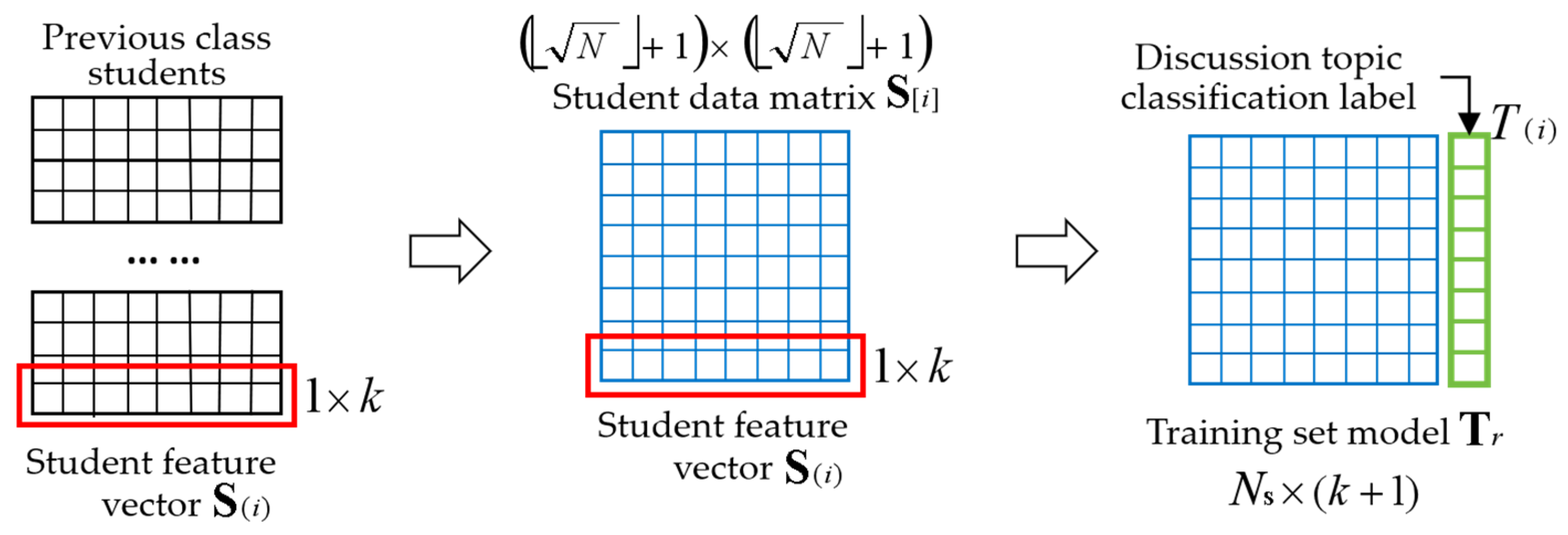
3.1.1. Training Set Model for Naive Bayes Machine Learning Algorithm

To establish the naive Bayes machine learning algorithm, it is necessary to select the individual students from the previous classes who meet the naive Bayes classification criteria and then construct the quantitative labels for the core elements of the practical teaching topics to determine the classified labels of the individual students. We construct the feature vector and the data matrix for the students in the previous classes, quantify the data matrix for the students in the previous class, select the individual students who meet the conditions of the naive Bayes machine learning algorithm, and then establish the training set model. We first construct the relevant definitions and then establish the naive Bayes machine learning training set model. Figure 1 shows the training set model of the constructed naive Bayes machine learning algorithm.

Definition 1.

The sample student $S_{(i)}$ and the student feature vector $S_{(i)}$. Naive Bayes machine learning is a supervised learning algorithm that requires collecting data from the previous courses and establishing a training set. We define an arbitrary student selected from the previous teaching class, who participates in the practical teaching and has feature attributes and interests, as the sample student, denoted as $S_{(i)}$. We construct a one-dimensional vector to store the teaching interest labels selected and quantified by the students. The dimension is denoted as $1\times k$, and its elements store the practical teaching topic elements. This vector is the student feature vector, denoted as $S_{(i)}$.

Definition 2.

The classification label $T_{(i)}$ for the discussion topic. The labels used for classification in supervised learning are the key elements of naive Bayes machine learning. We define the student classification label determined by the topic content in practical teaching as the classification label for constructing the naive Bayes machine learning, denoted as $T_{(i)}$. After determining the classification label, the student feature vector is expanded into dimension $1\times (k+1)$, and the last element of the vector stores the label $T_{(i)}$ .

Definition 3.

The student data matrix $S_{[i]}$. We select sample students from all the previous students who could be used as the training set for constructing the naive Bayes machine learning algorithm, and store them in a matrix in the order of a certain algorithm. We define the matrix as the student data matrix, denoted as $S_{[i]}$.

Definition 4.

The training set model $T_r$ for the naive Bayes machine learning. According to the storage rules for the feature labels and classification labels in the naive Bayes training set, the vector $S_{(i)}$  is topologically transformed to generate a training set for constructing the naive Bayes machine learning, denoted as $T_r$. The training set stores the student labels and classifications that have undergone data prepossessing.

The algorithm for constructing the training set model for the naive Bayes machine learning based on the previous student teaching data is as follows (Appendix A.1):

Step 1: Randomly select $N$ number of students $S_{(i)}$ from the previous classes, each of whom is an independent individual with independent and different interests, which meet the conditions $\forall S_{(i)}\cap \forall S_{(j)}=\varnothing$, $0<i,j\le N$ and $i,j,N\in N$. We initialize the $N$ number of students $S_{(i)}$ as $S_{(1)}$, $S_{(2)}$, …, $S_{(N)}$.

Step 2: Establish the feature vector $S_{(i)}$ for the students in the previous classes, $0<i\le N$, $i,N\in N$. A vector $S_{(i)}$ represents a student $S_{(i)}$. Formula (1) is the constructed vector model $S_{(i)}$.

$$S_{(i)}=\left[\begin{array}{ccccccc}{L}_{(1)},& \dots ,& L_{(i)},& \dots ,& L_{(k)},& |& T_{(i)}\end{array}\right]$$

(1)

Step 2.1: Determine the $k$ number of the core attributes $L_{(i)}$ for the practical teaching topics, $0<i\le k$, $i,k\in N$. Each core attribute $L_{(i)}$ is an independent feature that satisfies $\forall L_{(i)}\cap \forall L_{(j)}=\varnothing$. Attribute $L_{(i)}$ has a quantifiable interval or discrete value.

Step 2.2: Determine $p$ number of discussion topics based on the practical content and note it as a classification label $T_{(i)}$, $0<i\le p$, $i,p\in N$.

Step 2.3: Establish a $1\times (k+1)$ dimensional vector $S_{(i)}$ with row rank $rank{(S_{(i)})}_{ro}=1$ and column rank $rank{(S_{(i)})}_{co}=k+1$. The composition of the vector elements is as follows:

(1) The first element of the no. $k$ element stores attributes $L_{(i)}$, corresponding to the element $S_{(x,j)}=L_{(i)}$, $0<i,j\le k$, in which $x$ represents the no. $x$ student element.

(2) The no. $k+1$ element $T_{(i)}$ corresponds to the element $S_{(x,k+1)}=T_{(i)}$, $0<i\le p$, in which $x$ represents the no. $x$ student element.

Step 3: Establish the previous class student data matrix $S_{[i]}$. According to the number $N$ of students $S_{(i)}$, we set the row rank $rank{(S_{[i]})}_{ro}$ and column rank $rank{(S_{[i]})}_{co}$ of the $n\times n$ dimensional matrix, satisfying $rank{(S_{[i]})}_{ro}=⌊\sqrt{N}⌋+1$, $rank{(S_{[i]})}_{co}=⌊\sqrt{N}⌋+1$. Formula (2) is the constructed matrix model $S_{[i]}$.

$$S[i]=\left[\begin{array}{ccccc}{S}_{(1)}& \dots & S_{(r1)}& \dots & S_{(\max r1)}\\ \dots & \dots & S_{(r2)}& \dots & S^{(\max r2)}\\ \hspace{1em}& \dots & \hspace{1em}& \dots \\ \dots & \hspace{1em}& S_{(r\max )}& \hspace{1em}& S_{(\max r\max )}\end{array}\right]$$

(2)

Step 3.1: Store the $N$ number of marked students $S_{(i)}$ in the matrix $S_{[i]}$ in increasing order of rows $i$ and columns $j$. The storage status meets the following conditions:

(1) If $N<n\times n$, then the remaining $n\times n-N$ number of elements $S_{[i,j]}$ in the matrix $S_{[i]}$ are stored as 0;

(2) If $N=n\times n$, then the matrix $S_{[i]}$ is full rank.

Step 3.2: The elements $S_{[i,j]}$ in the matrix $S_{[i]}$ correspond to the students $S_{(i)}$, and the vectors $S_{(i)}$ are quantified based on the previous data records. For the student $S_{(i)}$, if any element $\forall S_{(i,j)}$ in the vector $S_{(i)}$ satisfies $S_{(i,j)}=0$, it indicates that the student has not participated in any classification or practical course. Then, there are:

(1) For $\forall S_{[i,j]}$ in the matrix $S_{[i]}$, if corresponding student $S_{(i)}~S_{(i)}$ is $\exists S_{(i,j)}=0$, then set $S_{[i,j]}=0$;

(2) For $\forall S_{[i,j]}$ in the matrix $S_{[i]}$, if corresponding student $S_{(i)}~S_{(i)}$ is $\forall S_{(i,j)}\ne 0$, then set $S_{[i,j]}=1$.

Step 3.3: Mark all the elements of $S_{[i,j]}=1$ in the matrix $S_{[i]}$ with a count of $N_S$. According to the modeling process, there is $N_S\le N$.

Step 4: Build the training set model for the naive Bayes machine learning. Construct a $N_S\times (k+1)$ dimensional matrix $T_r$ based on the vector $S_{(i)}$ dimension $1\times (k+1)$. Formula (3) is the constructed model $T_r$.

$$T_r=\left[\begin{array}{cccccc}{L}_{(S_{(1)},1)},& \dots ,& L_{(S_{(1)},i)},& \dots ,& L_{(S_{(1)},k)},& T_{(S_{(1)})}\\ L_{(S_{(2)},1)},& \dots ,& L_{(S_{(2)},i)},& \dots ,& L_{(S_{(2)},k)},& T_{(S_{(2)})}\\ \dots & \hspace{1em}& \dots & \hspace{1em}& \dots & \dots \\ L_{(S_{(NS)},1)},& \dots ,& L(S_{(NS)},i),& \dots ,& L(S_{(NS)},k),& T_{(S_{(Ns)})}\end{array}\right]$$

(3)

Step 4.1: Extract the quantified matrix $S_{[i]}$ and extract $N_S$ number of elements $S_{[i,j]}=1$.

Step 4.2: Define the $1\times (k+1)$ dimensional empty vector $S_{(i)}=0$ with the row rank $rank{(S_{(i)})}_{ro}=1$ and the column rank $rank{(S_{(i)})}_{co}=k+1$.

Step 4.3 Initialize the row $r_o=1$, $r_o=r_o+1$, and expand the rows of the vector $S_{(i)}$. If $r_o<N_s$, continue to execute. Note that $r_o=r_o+1$. If $r_o=N_s$, complete the execution, and output $T_r$.

Step 4.4: Store the quantified labels of the $N_S$ number of students into $T_r$. The storage rule is:

(1) The matrix row corresponds to one student vector $S_{(i)}~S_{(i)}$;

(2) The element $T_{r(i,j)}$ represents the no. $j$ attribute label $L_{(i)}$ of the no. $i$ student and satisfies the constraint condition $0<i\le N_s$, $0<j\le k$, $i,j,N_s,k\in N$;

(3) The last column $c_o=k+1$ of the matrix $T_r$ stores the noted classification labels $T_{(i)}$ of students $S_{(i)}~S_{(i)}$.

3.1.2. Class Grouping Algorithm

The establishment of the naive Bayes machine learning algorithm is based on the constructed training set $T_r$, with the goal of achieving student classification in the teaching class and grouping the practical teaching based on the classification results. Based on the $k$ number of core attributes $L_{(i)}$ determined by the practical teaching topics, the interest labels and classification labels of students in the previous classes, we construct the naive Bayes machine learning model to calculate the Bayesian posterior probability of each student belonging to the classification label $T_{(i)}$, achieving the classification of the students in the teaching class. According to the modeling principle of the naive Bayes machine learning algorithm, the constructed training set $T_r$ consists of two parts: one is the student interest label and the quantified module, namely the element ${T_r}_{(i,j)}$, $0<i\le N_s$, $0<j\le k$, $i,j,N_s,k\in N$; the second is the student classification label module, namely the last column $co=k+1$ of the matrix $T_r$. The columns in the training set $T_r$ are independent from each other, which meets the modeling requirements of the naive Bayes machine learning algorithm [39].

Definition 5.

The naive Bayes prior probability model $P(T_{(i)})$. For the student training set, it is one of the conditions used to construct the naive Bayes machine learning algorithm. It is defined as the probability of the classification  $T_{(i)}$  appearing in the total number $N$ of samples in the training set.

Definition 6.

The naive Bayes conditional probability density $P(S_{(x)}|T_{(i)})$. For the student training set, it is also one of the conditions used to construct the naive Bayes machine learning algorithm. It is defined as the probability of students $S_{(x)}$ and student feature labels $L_{(i)}$ appearing under the classification conditions $T_{(i)}$ .

Definition 7.

The naive Bayes posterior probability model $P(T_{(i)}|S_{(x)})$. The probability of classifying student $S_{(x)}$ into the classification label $T_{(i)}$. It is used to determine the final classification of the student $S_{(x)}$ .

Definition 8.

The feature vector ${S_{(x)}}^{\Delta }$ of the student to be classified. Based on the $1\times (k+1)$ dimensional feature vector $S_{(i)}$ of the previous class of students, we construct a $1\times k$ dimensional vector with the same attribute labels $L_{(i)}$  for storing and quantifying the feature labels of students to be classified. We define this vector as the feature vector of the student to be classified, denoted as ${S_{(x)}}^{\Delta }$ .

For an arbitrary student $S_{(x)}$ to be classified in the teaching class, the classification objective is to match the student $S_{(x)}$ with the training set model $T_r$ for the naive Bayes machine learning algorithm and the selected classification labels $T_{(i)}$ based on the previous classes and use the classification algorithm to classify the student $S_{(x)}$ into the classification $T_{(i)}$ with the highest Bayesian posterior probability value. The measuring of the interest tendency of the student $S_{(x)}$ to be classified by the naive Bayes machine learning algorithm is consistent with the prior probability and previous teaching experience. We suppose that $H$ is the assumption that the student $S_{(x)}$ is classified to a classification $T_{(i)}$, and the basic idea of constructing a classification model using Bayes’ theorem is to determine the Bayesian posterior probability $P(T_{(i)}|S_{(x)})$ of the assumption that the student $S_{(x)}$ is to be classified to a classification $T_{(i)}$. Formula (4) is the constructed Bayesian posterior probability model that is used to assume that the student $S_{(x)}$ belongs to a classification $T_{(i)}$.

$$P(T_{(i)}|S_{(x)})={\displaystyle \frac{P(S_{(x)}|T_{(i)})P(T_{(i)})}{P(S_{(x)})}}$$

(4)

For the topic classification $T_{(i)}$ determined by the practical teaching, $0<i\le p$, $i,p\in N$, the naive Bayes machine learning algorithm predicts that a student $S_{(x)}$ belongs to the classification $T_{(i)}$ with the highest posterior probability by calculating the Bayesian posterior probability. For the $p$ number of classifications $T_{(i)}$ set in the sample space, the condition for the student $S_{(x)}$ belonging to a certain classification $T_{(i)}$ is: if and only if $P(T_{(u)}|S_{(x)})>\forall P(T_{(v)}|S_{(x)})$, in which $0<u,v\le p$ and $u\ne v$. At this moment, the classification $T_{(u)}$ relating to the maximum Bayesian posterior probability $P(T_{(u)}|S_{(x)})$ is the maximum posteriori assumption. Based on the modeling principle, the naive Bayes machine learning algorithm for the student $S_{(x)}$ classification is constructed as follows (Appendix A.2).

Step 1: Determine the quantified vector ${S_{(x)}}^{\Delta }$ of the student to be classified, which will be used to construct the naive Bayes machine learning model.

Step 2: Perform the equivalent simplification on the Bayesian posterior probability model.

Step 2.1: Without considering the conditional probability constraints, the possibility of the student $S_{(x)}$ in any class $\forall T_{(i)}$ is identical. Define the probability $P(S_{(x)})$ of the student $S_{(x)}$ for all classes $T_{(i)}$ as constant, i.e., $P(S_{(x)})=const$.

Step 2.2: Simplify the Bayesian posterior probability model $P(T_{(i)}|S_{(x)})$ and convert it to calculate the value $P(S_{(x)}|T_{(i)})P(T_{(i)})$.

Step 2.3: Set ${\delta }_{(S_{(x)})}=P(S_{(x)}|T_{(i)})P(T_{(i)})$. Calculating and comparing ${\delta }_{(S_{(x)})}$ is equivalent to calculating $P(T_{(i)}|S_{(x)})$.

Step 3: Retrieve the training set model $T_r$ and construct the prior probability model $P(T_{(i)})$ for the classification labels.

Step 3.1: Mark the students $S_{(i)}$ in the model $T_r$ who belong to the classification $T_{(i)}$ and record $S_{(i)}\in T_{(i)}$.

Step 3.2: Initialize $r_o=1$, $N_{T_{(i)}}=0$, set the number of students as $N_{T_{(i)}}$, $S_{(i)}\in T_{(i)}$, and determine the rows of the matrix $T_r$: (1) if $S_{(i)}\in T_{(i)}$, then $N_{T_{(i)}}=N_{T_{(i)}}+1$; (2) if $S_{(i)}\notin T_{(i)}$, then $N_{T_{(i)}}=N_{T_{(i)}}+0$.

Step 3.3: Iterate $r_o=r_o+1$, determine whether row $r_o$ related to $S_{(i)}$ meets $S_{(i)}\in T_{(i)}$, and include $N_{T_{(i)}}$.

Step 3.4: Determine the termination conditions: (1) if $r_o=N_S$, the searching ends, output the current $N_{T_{(i)}}$; (2) if $r_o<N_S$, continue searching.

Step 3.5: Build a prior probability model for student classification, as shown in Formula (5).

$$P(T_{(i)})={\displaystyle \frac{N_{T_{(i)}}}{N_S}}$$

(5)

Step 3.6: Repeat steps 3.1 to 3.5, traverse $T_{(i)}~i\in \left\{i|0<i\le p\right\}$, and calculate the prior probability for each $T_{(i)}$.

Step 4: Introduce ${S_{(x)}}^{\Delta }$ and quantify the labels $L_{(i)}$ to construct the conditional probability density model $P(S_{(x)}|T_{(i)})$.

Step 4.1: If the attribute labels in the matrix $T_r$ satisfy $\forall L_{(S_{(i)},i)}\cap \forall L_{(S_{(i)},i)}=\varnothing$, construct a conditional probability density function $P(S_{(x)}|T_{(i)})$, as shown in Formula (6).

$$P(S_{(x)}|T_{(i)})={\displaystyle \prod _{u=1}^{k}P(L_{(u)}|T_{(i)})}$$

(6)

Step 4.2: Estimate the probability $P(L_{(u)}|T_{(i)})$. Each label in the matrix $T_r$ satisfies the condition $\forall L_{(S_{(i)},i)}\cap \forall L_{(S_{(i)},i)}=\varnothing$, which means that each label is a discrete feature. The probability estimate $P(L_{(u)}|T_{(i)})$ is constructed as Formula (7), in which $w_{(i,u)}$ is the number of students with attribute labels $L_{(u)}$ in the classification $T_{(i)}$, and $w_{(i)}$ is the number of students in the classification $T_{(i)}$.

$$P(L_{(u)}|T_{(i)})={\displaystyle \frac{w_{(i,k)}}{w_{(i)}}}$$

(7)

Step 4.3: When counting the number of label $L_{(u)}$ as $w_{(i,u)}=0$, in order to avoid calculating the conditional probability density value as 0, a perturbation factor $\sigma$ is introduced as an adjustment when calculating the number of the label as $w_{(i,u)}=0$. Then, a conditional probability density model is constructed as shown in Formula (8).

$$P(S_{(x)}|T_{(i)})={\displaystyle \prod _{u=1}^k\left(\frac{w_{(i,u)}}{w_{(i)}}+\sigma \right)}, \forall \left({\displaystyle \frac{w_{(i,u)}}{w_{(i)}}}+\sigma \right)<1$$

(8)

Step 5: Calculate the transformation value ${\delta }_{(S_{(x)})}$ for the Bayesian posterior probability, traversing $T_{(i)}~i\in \left\{i|0<i\le p\right\}$, and determine the classification $T_{(i)}$ with the $\max {\delta }_{(S_{(x)})}$ as the classification that the student $S_{(x)}$ belongs to.

3.2. Teaching Recommendation Model Based on Improved k-NN Data Mining Algorithm

The naive Bayes machine learning algorithm determines the classification $T_{(i)}$ of the students in the teaching class, and based on the determined student classification, the teachers encode and group the students in the class. According to the inherent logic of the naive Bayes machine learning algorithm, the students in the same classification tend to have a high degree of closeness in their interest tendencies, while the students in the different classifications tend to have a low degree of closeness in their interest tendencies. According to the course design process, the teachers need to determine the specific practical topic content for each group based on the grouping. Scientific and quantitative recommendation and decision making is the best mode for accurately determining the practical topic content for each group, ensuring that the recommended practical topic content can accurately match the interests of each student in the group. Due to the inclusion of multiple students in each group $T_{(i)}$, the construction of the practical topic recommendation algorithm must consider the precise interests of all students. From the perspective of recommendation algorithm design, it is necessary to construct a collective recommendation model [40]. Based on this fundamental principle, we construct a teaching recommendation model based on the improved k-NN data mining algorithm.

The basic idea of the modeling is as follows. We set the classification result as the $p$ number of groups $T_{(i)}$. Each classification $T_{(i)}$ represents one interest, and the number of students in each group $T_{(i)}$ is $N_{T_{(i)}}$. The teacher determines $h_i$ number of discussion topics $G_{(j)}$ for each group $T_{(i)}$, $0<j\le h_{(i)}$, $j,h_{(i)}\in N$. We build a k-NN data mining algorithm between $N_{T_{(i)}}$ number of students and $h_{(i)}$ number of discussion topics in a group $T_{(i)}$, output $n$ number of the most matching topics for each student, and then find the $k$ number of topics with the best intersection among the $n$ number of topics as the recommended topics for the group $T_{(i)}$ of students. The model outputs the recommended topics for other groups $T_{(i)}$ by using the same algorithm until the recommendations for the $p$ number of groups are completed [41].

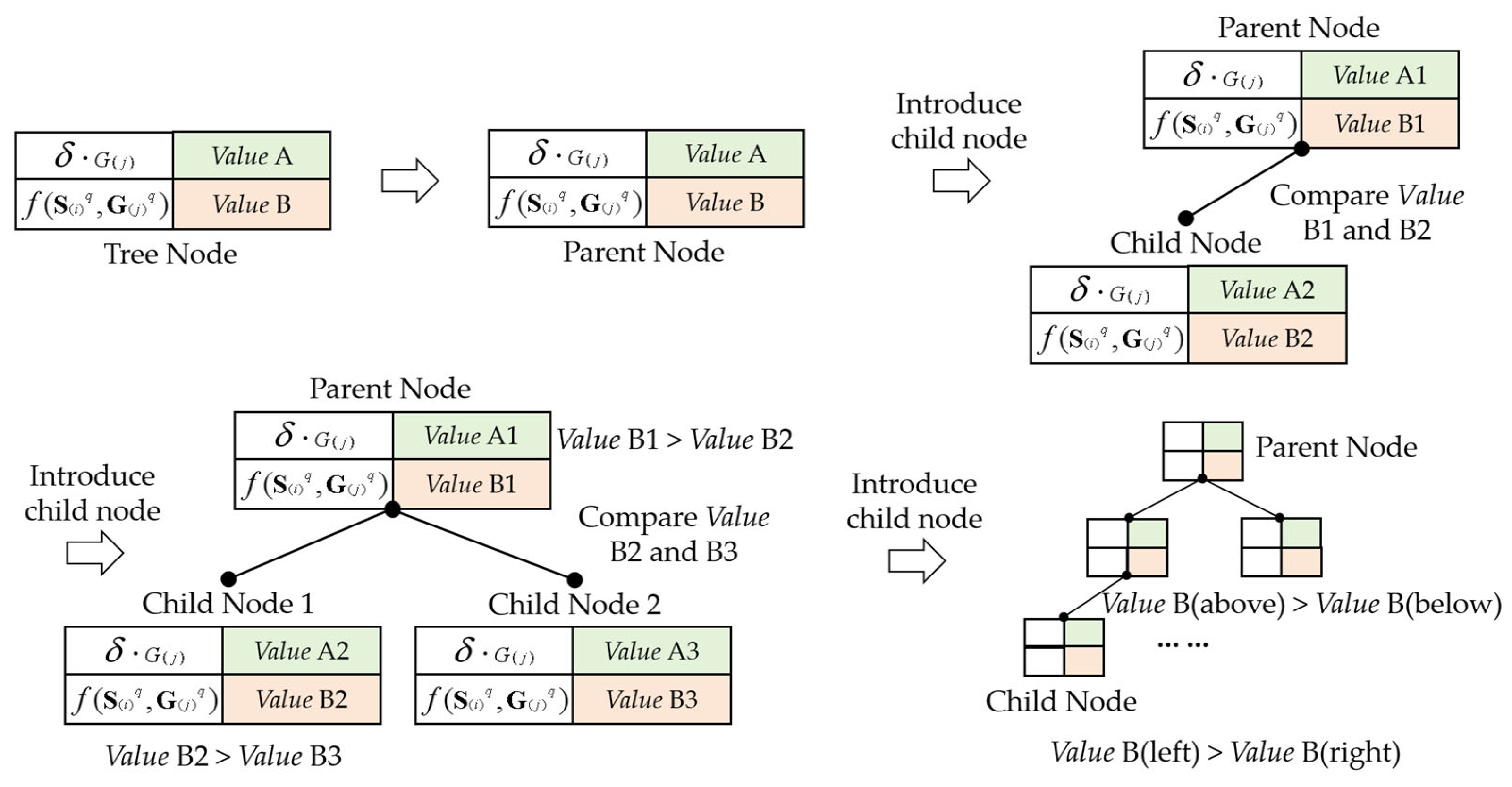
3.2.1. The Modeling of the Complete Binary Encoding Tree for Discussion Topic

According to the modeling concept, we confirm some Definitions for the algorithm. Firstly, the algorithm is constructed to match the individual students $S_{(i)}$ in the group $T_{(i)}$ with the discussion topics $G_{(j)}$, and the optimal complete binary encoding tree model for the discussion topic is established.

Definition 9.

The discussion topic feature vector $G_{(j)}$. For the $h_{(i)}$ number of discussion topics $G_{(j)}$ designed for the group $T_{(i)}$, the containing labels of each discussion topic $G_{(j)}$ have a matching relationship with the labels $S_{(i,t)}$ contained in the $1\times k$ dimensional student interest feature vector $S_{(i)}$. The $1\times k$ dimensional vector composed of $k$ number of quantified labels used to express the characteristics of the discussion topic is defined as the discussion topic feature vector, denoted as $G_{(j)}$. The vector elements are labels $G_{(j,t)}$, $0<j\le h_{(i)}$, $0<t\le k$, and $j,h_{(i)},t,k\in N$ .

Definition 10.

The quantization vector ${S_{(i)}}^q$ and the quantization vector ${G_{(j)}}^q$. We quantify and normalize the elements $S_{(i,t)}$ of the vector $S_{(i)}$ based on the interests of the individual students $S_{(i)}$, and the resulting quantified vector is denoted as ${S_{(i)}}^q$, in which the normalized elements are denoted as $S_{(i,t)}$. For the feature vector of the discussion topic, the elements $G_{(j,t)}$ are quantified and normalized based on the topic characteristics, and the resulting quantified vector is denoted as ${G_{(j)}}^q$, in which the normalized elements are denoted as $g_{(i,t)}$ .

Definition 11.

The discussion topic weight $\delta {\cdot }_{G(j)}$. The feature vector of the discussion topic describes the degree to which a certain discussion content covers the requirements of the practical teaching under the specific practical teaching conditions. The reciprocal of the modulus of the quantified vector ${G_{(j)}}^q$ of the discussion topic is defined as the discussion topic weight $\delta {\cdot }_{G_{(j)}}$, quantified as $\delta {\cdot }_{G_{(j)}}={\left|{G_{(j)}}^q\right|}^{-1}$. It is the measurement value that covers the requirements of the practical teaching. The higher the weight value is, the higher the coverage will be.

Definition 12.

The discussion topic matching model $f({S_{(i)}}^q,{G_{(j)}}^q)$. Based on the matching feature between the student interest feature vector $S_{(i)}$ and the discussion topic feature vector $G_{(j)}$, a matching model based on the quantization vector ${S_{(i)}}^q$ and ${G_{(j)}}^q$ is constructed to express the matching measurement value between the individual interest of no. $i$ student $S_{(i)}$ in the group $T_{(i)}$ and the no. $j$ discussion topic $G_{(j)}$. Formula (9) is the constructed discussion topic matching model.

$$f({S_{(i)}}^q,{G_{(j)}}^q)={\left[{\displaystyle \sum _{t=1}^k{\left(s_{(i,t)}-g_{(i,t)}\right)}^q}\right]}^{-{\displaystyle \frac{1}{q}}}$$

(9)

Definition 13.

The discussion topic spatial coordinate system $xo{y}^{G_{(i)}}$ and the spatial coordinates $(x_{G_{(i)}},y_{G_{(i)}})$. Based on the discussion topic weight $\delta {\cdot }_{G_{(j)}}$ and the discussion topic matching model $f({S_{(i)}}^q,{G_{(j)}}^q)$, we quantitatively model the spatial distribution of the discussion topics $G_{(j)}$ included in student group $T_{(i)}$. We construct a spatial coordinate system for the discussion topics with weights $\delta {\cdot }_{G_{(j)}}$ as the abscissa and function values $f({S_{(i)}}^q,{G_{(j)}}^q)$ as the ordinate, denoted as $xo{y}^{G(i)}$. The discussion topic is represented by a coordinate point, whose coordinates are denoted as $(x_{G_{(i)}},y_{G_{(i)}})$, in which $x_{G_{(i)}}={\delta }_{\cdot G_{(j)}}$,  $y_{G_{(i)}}=f({S_{(i)}}^q,{G_{(j)}}^q)$. Figure 2 shows the constructed discussion topic spatial coordinate system:  Figure 2a shows the constructed spatial coordinate system $xo{y}^{G_{(i)}}$, and Figure 2b shows an example of the quantified coordinate system containing the discussion topic points.

Definition 14.

The optimal complete binary encoding tree model $H_T$ for the discussion topic. The goal of the optimal complete binary tree model is to achieve the ordered storage of parent node and child nodes, output the optimal sorted tree structure, and extract the optimal nodes. We simulate the generation rules of the optimal complete binary tree. Based on the discussion topic spatial coordinate system $xo{y}^{G(i)}$ and the spatial coordinates $(x_{G_{(i)}},y_{G_{(i)}})$, we treat the spatial coordinates $(x_{G_{(i)}},y_{G_{(i)}})$ as the codes of the discussion topic in the coordinate system $xo{y}^{G(i)}$ and construct the complete binary tree with the optimal parent node. This tree is defined as the optimal complete binary encoding tree model for the discussion topic, denoted as $H_T$ . Figure 3  shows the basic generation rules and the logical structure of the tree model $H_T$. Based on the Definition, the rules and logical structure are generated in Figure 3.

The algorithm steps for constructing the optimal complete binary encoding tree model for the discussion topic are as follows (Appendix A.3).

Step 1: Select the individual student $S_{(i)}$ from the group $T_{(i)}$. Quantify and output ${S_{(i)}}^q$. Quantify and output $h_{(i)}$ number of ${G_{(j)}}^q$ for $h_{(i)}$ number of the topics $G_{(j)}$ in the group $T_{(i)}$ and encode the discussion topics $G_{(j)}$.

Step 1.1: Determine the basic structure of the discussion topic $G_{(j)}$ in the coordinate system $xo{y}^{G_{(i)}}$, including the head-word $h_{ead}$ and suffix-word $S_{uffix}$. The storage structure is as follows:

{$<h_{ead}>$: discussion topic weight: ${\delta \cdot }_{G_{(j)}}$} & {$<S_{uffix}>$: discussion topic matching value: ${S_{(i)}}^q,{G_{(j)}}^q)$}

Step 1.2: Initialize the counter $count=0$, which is the number of times the discussion topic $G_{(j)}$ has been traversed.

Step 1.3: Take $j=1$, initialize the first topic $G_{(1)}$, and generate the nodes for $G_{(1)}$.

(1) Extract ${G_{(1)}}^q$, calculate ${\delta \cdot }_{G_{(1)}}$, and store ${\delta \cdot }_{G_{(1)}}$ to the related head-word $h_{ead}$ for $G_{(1)}$;

(2) Extract ${S_{(i)}}^q$, calculate $f({S_{(i)}}^q,{G_{(1)}}^q)$, and store $f({S_{(i)}}^q,{G_{(1)}}^q)$ to the corresponding suffix-word $S_{uffix}$ for $G_{(1)}$;

(3) Complete the storage and generate the storage structure for node $G_{(1)}$;

(4) Note $count=count+1$: (i) if $count<h_{(i)}$, continue searching; (ii) if $count=h_{(i)}$, the node searching ends, and the algorithm ends.

Step 1.4: For any $\forall j$, return to Step 1.3 to initialize the no. $j$ topic $G_{(j)}$ and generate node $G_{(j)}$. Note $count=count+1$: (i) if $count<h_{(i)}$, continue searching; (ii) if $count=h_{(i)}$, the node searching ends, and the algorithm ends.

Step 1.5: Iterate the index $count$, and stop the iterating when $count=h_{(i)}$. Output the node storage structures for $h_{(i)}$ number of discussion topics $G_{(j)}$.

Step 1.6: Based on the node storage structures for $h_{(i)}$ number of discussion topics $G_{(j)}$, establish the spatial coordinate system $xo{y}^{G_{(i)}}$ of the discussion topic under the condition of the individual student $S_{(i)}$ interest vector ${S_{(i)}}^q$.

Step 2: Randomly select any topic $\forall G_{(j1)}$ and store it in the parent node $H_{T(1,1)}$ of the model $H_T$. Randomly select another topic $\forall G_{(j2)}$ and make the following comparison, in which $f_{(j)}$ represents $f({S_{(i)}}^q,{G_{(j)}}^q)$, the number $j$ represents the no. $j$ topic $G_{(j)}$, and each function value $f_{(j)}$ has the same ${S_{(i)}}^q$.

(1) If $f_{(j1)}\ge f_{(j2)}$, keep the topic $G_{(j1)}$ storage $H_{T(1,1)}$ unchanged and store $G_{(j2)}$ in the left child node $H_{T(2,1)}$ of the second layer;

(2) If $f_{(j1)}<f_{(j2)}$, delete $H_{T(1,1)}$, store $G_{(j2)}$ in the parent node $H_{T(1,1)}$ of the model $H_T$, and store $G_{(j1)}$ in the left child node $H_{T(2,1)}$ of the second layer.

Step 3: Introduce arbitrary $\forall G_{(j3)}$ and make the following comparison:

(1) If $f_{(j1)}\ge f_{(j2)}$:

① If $f_{(j1)}\ge f_{(j2)}\ge f_{(j3)}$, store $G_{(j1)}$ and $G_{(j2)}$ to $H_{T(1,1)}$ and $H_{T(2,1)}$, and store $G_{(j3)}$ to the child node $H_{T(2,2)}$ on the right side of the second row;

② If $f_{(j1)}\ge f_{(j3)}>f_{(j2)}$, store $G_{(j1)}$ and $G_{(j3)}$ to $H_{T(1,1)}$ and $H_{T(2,1)}$, and store $G_{(j2)}$ to the child node $H_{T(2,2)}$ on the right side of the second row;

③ If $f_{(j3)}>f_{(j1)}\ge f_{(j2)}$, store $G_{(j3)}$ and $G_{(j1)}$ to $H_{T(1,1)}$ and $H_{T(2,1)}$, and store $G_{(j2)}$ to the child node $H_{T(2,2)}$ on the right side of the second row;

(2) If $f_{(j1)}<f_{(j2)}$:

① If $f_{(j3)}\le f_{(j1)}<f_{(j2)}$, store $G_{(j2)}$ and $G_{(j1)}$ to $H_{T(1,1)}$ and $H_{T(2,1)}$, and store $G_{(j3)}$ to the child node $H_{T(2,2)}$ on the right side of the second row;

② If $f_{(j1)}<f_{(j3)}\le f_{(j2)}$, store $G_{(j2)}$ and $G_{(j3)}$ to $H_{T(1,1)}$ and $H_{T(2,1)}$, and store $G_{(j1)}$ to the child node $H_{T(2,2)}$ on the right side of the second row;

③ If $f_{(j1)}<f_{(j2)}<f_{(j3)}$, store $G_{(j3)}$ and $G_{(j2)}$ to $H_{T(1,1)}$ and $H_{T(2,1)}$, and store $G_{(j1)}$ to the child node $H_{T(2,2)}$ on the right side of the second row.

Step 4: Introduce any $\forall G_{(jc)}$, $4<c\le h_{(i)}$. Calculate the current $f_{(jc)}$ corresponding to $G_{(jc)}$, compare $f_{(j1)}$~$f_{(jc)}$, and continue storing by the following storage rules.

(1) Arbitrary node $H_{T(u,v)}$ can have a maximum of two child nodes $H_{T(u+1,*)}$ and a minimum of zero child nodes;

(2) Regarding the binary tree storage rule, any row $u$ of the tree $H_T$ contains $2^{u-1}$ number of child nodes, and $G_{(j1)}$~$G_{(jc)}$ must be stored in the previous $c$ number of nodes in the tree $H_T$, satisfying the following:

① The number of nodes that store $G_{(j)}$ meets the requirement ${\displaystyle {\sum }_{u=1}^{\max u}{2}^{u-1}}\ge c$. The $\max u$ represents the maximum row that is used to store $G_{(j)}$;

② For any node $\forall H_{T(u,v)}$ for $G_{(j)}$, its left node $H_{T(u,v-1)}$ must meet the criteria $H_{T(u,v-1)}\ne \varnothing$;

③ For any node $\forall H_{T(u,v)}$ for $G_{(j)}$, its right node $H_{T(u,v+1)}$ must meet the following:

(i) If the last $G_{(jc)}$ is currently stored in $H_{T(u,v)}$, the node $H_{T(u,v+1)}$ on the right does not exist;

(ii) If the current node $H_{T(u,v)}$ is not the last $G_{(jc)}$, the right node continues to store, satisfying the condition $H_{T(u,v+1)}\ne \varnothing$.

④ If the row $u$ contains the child node that stores $G_{(j)}$, then all nodes in the previous $u-1$ rows of the tree $H_T$ satisfy the condition $H_{T(u,v)}\ne \varnothing$.

(3) Any node $H_{T(u,v)}$ satisfies the following:

① The stored $H_{T(u,v)}$ of $G_{(j)}$ corresponds to $f_{(jm)}$, the stored $G_{(j)}$ of child nodes $H_{T(u+1,2v-1)}$ and $H_{T(u+1,2v)}$ correspond to $f_{(jk)}$ and $f_{(jd)}$, and there is $f_{(jm)}\ge f_{(jk)}\ge f_{(jd)}$;

② The stored $H_{T(u,v)}$ of $G_{(j)}$ corresponds to $f_{(jm)}$, the stored $G_{(j)}$ of left node $H_{T(u,v-1)}$ corresponds to $f_{(jk)}$, the stored $G_{(j)}$ of right node $H_{T(u,v+1)}$ corresponds to $f_{(jd)}$, and there is $f_{(jk)}\ge f_{(jm)}\ge f_{(jd)}$.

Step 5: Continue storing $G_{(jc)}$ according to the algorithm from Step 1 to Step 4 until the searching stops at the end of traversal $c=h_{(i)}$. The algorithm ends, producing output $H_T$.

3.2.2. Recommendation Model Based on the Improved k-NN Data Mining Algorithm

For any student group $T_{(i)}$, the construction of the k-NN data mining algorithm is based on the optimal complete binary encoding tree of the discussion topic. Firstly, we establish the encoding trees $H_T$ for all the individual students $S_{(i)}$ in the group $T_{(i)}$ and search for the first $n$ number of optimal matching topics $G_{(j)}$ based on the encoding tree. Secondly, based on the determined $n$ number of optimal matching topics $G_{(j)}$ for $N_{T_{(i)}}$ number of students $S_{(i)}$, the group $T_{(i)}$ is used as a team discussion group to find out the $k$ number of common optimal nearest neighbor topics for $N_{T_{(i)}}$ number of students $S_{(i)}$ and to recommend them as the optimal topics for the group $T_{(i)}$. Finally, the model outputs the recommended topics for each group $T_{(i)}$ generated for the class, and then the teacher and the students jointly determine the practical discussion topic for the practical course [42]. Based on the modeling principle, we construct the related Definitions for the algorithm.

Definition 15.

The optimal topic vector $U_{(i,j)}$ for the student $S_{(i)}$. Regarding the constructed student optimal encoding tree $H_T$, the previous $n$ number of nodes are selected starting from the parent node $H_{T(1,1)}$ as the topics that best match the student $S_{(i)}$. When the value reaches until the node $H_{T(u,v)}$, it satisfies the requirement $n={\displaystyle {\sum }_{u=1}^{u-1}{2}^{u-1}}+v$. Construct a $1\times n$ dimensional vector to store the selected $n$ number of nodes corresponding to the topics $G_{(j)}$ from the tree $H_T$. Define this vector as the optimal topic vector for the student $S_{(i)}$, denoted as $U_{(i,j)}$. The $i$ in the vector represents the no. $i$ student, and the $j$ in the vector represents the no. $j$ topic $G_{(j)}$ .

Definition 16.

The student optimal topic matrix $U_{N_{T(i})\times n}$ for the student $S_{(i)}$. Each student $S_{(i)}$ corresponds to the $n$ number of the most matched topics $G_{(j)}$, and if the group $T_{(i)}$ contains $N_{T_{(i)}}$ number of students $S_{(i)}$, a $N_{T_{(i)}}\times n$ dimensional matrix is constructed to store all the topics corresponding to $N_{T_{(i)}}$ number of students $S_{(i)}$. The matrix $U_{N{T}_{(i)}\times n}$ satisfies the following conditions:

(1) The row rank is $rank{(U_{N_{T_{(i)}}\times n})}_{ro}=N_{T_{(i)}}$, and the column rank is $rank{(U_{N_{T_{(i)}}\times n})}_{co}=n$;

(2) The row corresponds to one student $S_{(i)}$, and the column element represents the topic $G_{(j)}$;

(3) The rows ${\forall r}_{o(x)}$ and ${\forall r}_{o(y)}$ are not linearly related, and the columns ${\forall c}_{o(x)}$ and ${\forall c}_{o(y)}$ are not linearly related;

(4) Any element is a non-zero element;

(5) A matrix $U_{N_{T_{(i)}\times n}}$ corresponds to a group $T_{(i)}$.

Definition 17.

The discussion topic interest intensity $f_{G_{(j)}}$. For any group $T_{(i)}$ and the related matrix $U_{N_{T_{(i)}}\times n}$, we construct an algorithm to iterate the frequency of each topic $G_{(j)}$ appearing in the matrix $U_{N_{T_{(i)}}\times n}$, and the frequency of $G_{(j)}$ is defined as the discussion topic interest intensity, denoted as $f_{G_{(j)}}$. Normalize the intensity $f_{G_{(j)}}$ to obtain the interest intensity weight with a value range of $0<f_{G_{(j)}}<1$.

Definition 18.

The discussion topic recommendation vector $R_{(i,j)}$. Extract the $k$ number of topics $G_{(j)}$ with the highest intensity $f_{G_{(j)}}$ from the matrix $U_{N_{T_{(i)}}\times n}$ and store them in a $1\times k$ dimensional vector in order of decreasing intensity. We define this vector as the discussion topic recommendation vector, denoted as $R_{(i,j)}$. The $i$ represents the no. $i$ group $T_{(i)}$, and the $j$ represents the no. $j$ topic $G_{(j)}$ .

Based on the basic idea and the related Definitions of the algorithm model, we construct a recommendation model based on the improved k-NN data mining algorithm to recommend the optimal discussion topics $G_{(j)}$ for each student group $T_{(i)}$. The constructed algorithm is as follows (Appendix A.4):

Step 1: Determine the group $T_{(i)}$ and the student $S_{(i)}$, and quantify the student interest vector ${S_{(i)}}^q$ and the topic vector ${G_{(j)}}^q$. Introduce the optimal complete binary encoding tree algorithm for the discussion topics and output the individual encoding trees $H_{T^{(i)}}$ for the students $S_{(i)}$.

Step 1.1: Generate the encoding tree $H_{T^{(1)}}$ for the student $S_{(1)}$, and mark the previous $n={\displaystyle {\sum }_{u=1}^{u-1}{2}^{u-1}}+v$ number of nodes including the parent node $H_{T(1,1)}$, in which $u$ is the maximum row of the current tree with $n$ number of nodes, while $v$ is the maximum element number in the no. $u$ row in the tree.

Step 1.2: Regarding the same algorithm, generate the encoding trees ${H_T}^{(2)}$, ${H_T}^{(3)}$, …, ${H_T}^{(N_{T_{(i)}})}$ for the students $S_{(2)}$, $S_{(3)}$, …, $S_{(N_{T_{(i)}})}$, and mark the previous $n={\displaystyle {\sum }_{u=1}^{u-1}{2}^{u-1}}+v$ number of nodes in each tree separately.

Step 2: Output the optimal topic vector $U_{(i,j)}$ of the student $S_{(i)}$. Based on each encoding tree ${H_T}^{(i)}$ of the student $S_{(i)}$ and labeled $n$ number of nodes, extract the corresponding topics $G_{(j)}$ for $n$ number of nodes and construct the vector $U_{(i,j)}$.

Step 2.1: Take the $n$ number of optimal topics $G_{(j)}$ from the encoding tree ${H_T}^{(1)}$ of the student $S_{(1)}$ and store them in $1\times k$ dimensional vector $U_{(1,j)}$.

Step 2.2: Take the $n$ number of optimal topics $G_{(j)}$ of the corresponding encoding trees ${H_T}^{(2)}$, ${H_T}^{(3)}$, …, ${H_T}^{(N_{T_{(i)}})}$ of the students $S_{(2)}$, $S_{(3)}$, …, $S(N_{T_{(i)}})$, and store them in $1\times k$ dimensional vector $U_{(i,j)}$, in which $i=2,3,\dots ,N_{T_{(i)}}$.

Step 3: Initialize the matrix $U_{N_{T_{(i)}}\times n}=0$ and initialize the counter $count=0$. Generate the full rank matrix $U_{N_{T_{(i)}}\times n}$:

Step 3.1: Take the element $U_{(1,j)}$ and store $U_{(1,1)}$~$U_{(1,n)}$ in the first row of the matrix in sequence, so that the first row is full rank. Note $count=count+1$.

Step 3.2: Take the element $U_{(2,j)}$ and store $U_{(2,1)}$~$U_{(2,n)}$ in the second row of the matrix in sequence, so that the second row is full rank. Note $count=count+1$.

Step 3.3: In line with the same storage rules, take the element $U_{(i,j)}$, and store the $U_{(i,1)}$~$U_{(i,n)}$ in the no. $i$ row of the matrix in sequence, so that the no. $i$ row is full rank, in which $i$ traverses $3<i\le N_{T_{(i)}}$. Note $count=count+1$ until the traversal is completed when $count=N_{T_{(i)}}$; then, the storing process ends.

Step 4: Build a baseline vector $B$ containing $h_{(i)}$ number of the discussion topics $G_{(j)}$. The dimension of the vector $B$ is $1\times h_{(i)}$, and the vector element $B_{(j)}$ corresponds to the stored $G_{(j)}$. Introduce vector $B$ to scan the matrix $U_{N_{T_{(i)}}\times n}$.

Step 4.1: The row code of the matrix $U_{N_{T_{(i)}}\times n}$ is $u$, the column code is $v$, and the matrix elements are $U(u,v)$. According to the matrix Definition $U_{N_{T_{(i)}}\times n}$, there are $0<u\le N_{T_{(i)}}$, $0<v\le n$, and $u,N_{T_{(i)}},v,n\in N$.

Step 4.2: Initialize the counter $count=0$. Take the first element $B_{(1)}~G_{(j)}$ of the vector $B$ and make the following judgment:

(1) For matrix $U_{N_{T_{(i)}}\times n}$, take $u=1$ and traverse $0<v\le n$:

(i) If $U_{(1,1)}=B_{(1)}$, then $count=count+1$; if $U_{(1,1)}\ne B_{(1)}$, then $count=count+0$.

(ii) If $U_{(1,2)}=B_{(1)}$, then $count=count+1$; if $U_{(1,2)}\ne B_{(1)}$, then $count=count+0$.

(iii) Using the same iterative method, if $U_{(1,v)}=B_{(1)}$, then $count=count+1$; if $U_{(1,v)}\ne B_{(1)}$, then $count=count+0$. Until the traversal is complete, when $v=n$, output $count$ and note $coun{t}_{(1)}$.

(2) For matrix $U_{N_{T_{(i)}}\times n}$, take $u=2$, and traverse $0<v\le n$. Iterate over the elements $U_{(2,v)}$ in the second row of the matrix, and output $count$, denoted as $coun{t}_{(2)}$.

(3) Follow steps (1)–(2) to traverse all rows $2<u\le N_{T_{(i)}}$ of the matrix $U_{N_{T_{(i)}}\times n}$ and output $coun{t}_{(3)}~coun{t}_{(N_{T_{(i)}})}$ separately.

(4) Iterate to calculate $\delta (1)={\displaystyle {\sum }_{i=1}^{N_{T_{(i)}}}coun{t}_{(i)}}$, and denote $\delta (1)$ as the interest intensity ${f_{G_{(j)}}}^{[1]}$ of the element $B_{(1)}$.

Step 4.3: Initialize the counter $count=0$. Take the second element $B_{(2)}~G_{(j)}$ of the vector $B$, iterate in line with the same algorithm as in Step 4.2, and output $\delta (2)$ as the interest intensity ${f_{G_{(j)}}}^{[2]}$ of the element $B_{(2)}$.

Step 4.4: Using the same algorithm, output the interest intensity ${f_{G_{(j)}}}^{[i]}$ of the element $B_{(i)}$. Traverse $2<i\le h_{(i)}$, complete the iteration, and output ${f_{G_{(j)}}}^{[h(i)]}$ before the searching ends. Output the quantified vector $B$.

Step 4.5: Calculate the normalized interest intensity weight ${{\overline{f}}_{G_{(j)}}}^{[i]}$. Formula (10) is the constructed interest intensity weight model ${{\overline{f}}_{G_{(j)}}}^{[i]}$.

$${{\overline{f}}_{G_{(j)}}}^{[i]}={\displaystyle \frac{{f_{G_{(j)}}}^{[i]}}{{\displaystyle {\sum }_{i=1}^n{f_{G_{(j)}}}^{[i]}}}}$$

(10)

Step 5: Build a complete binary tree $T_B$ based on the vector $B$ by the following algorithm:

Step 5.1: Take $B_{(1)}$ and store in the parent node $T_{B_{(1,1)}}$ of the tree. Take $B_{(2)}$ and make a judgment:

(1) If ${f_{G_{(j)}}}^{[1]}\ge {f_{G_{(j)}}}^{[2]}$, store $B_{(2)}$ in the left child node $T_{B_{(2,1)}}$ of the second layer.

(2) If ${f_{G_{(j)}}}^{[1]}<{f_{G_{(j)}}}^{[2]}$, delete $T_{B_{(1,1)}}$, and store $B_{(2)}$ to the parent node $T_{B_{(1,1)}}$ and store $B_{(1)}$ to the left child node $T_{B_{(2,1)}}$ of the second layer.

Step 5.2: Take $B_{(3)}$ and make a judgment:

(1) If ${f_{G_{(j)}}}^{[1]}\ge {f_{G_{(j)}}}^{[2]}$.

① If ${f_{G_{(j)}}}^{[1]}\ge {f_{G_{(j)}}}^{[2]}\ge {f_{G_{(j)}}}^{[3]}$, keep $T_{B_{(1,1)}}$ and $T_{B_{(2,1)}}$, and store $B_{(3)}$ to the right child node $T_{B_{(2,2)}}$;

② If ${f_{G_{(j)}}}^{[1]}\ge {f_{G_{(j)}}}^{[3]}>{f_{G_{(j)}}}^{[2]}$, store $B_{(3)}$ to $T_{B_{(2,1)}}$, and store $B_{(2)}$ to $T_{B_{(2,2)}}$;

③ If ${f_{G_{(j)}}}^{[3]}>{f_{G_{(j)}}}^{[1]}\ge {f_{G_{(j)}}}^{[2]}$, delete $T_{B_{(1,1)}}$ and $T_{B_{(2,1)}}$, and then store $B_{(3)}$ to $T_{B_{(1,1)}}$ and store $B_{(1)}$ and $B_{(2)}$ to $T_{B_{(2,1)}}$ and $T_{B_{(2,2)}}$.

(2) If ${f_{G_{(j)}}}^{[1]}<{f_{G_{(j)}}}^{[2]}$.

① If ${f_{G_{(j)}}}^{[3]}\le {f_{G_{(j)}}}^{[1]}<{f_{G_{(j)}}}^{[2]}$, keep $T_{B_{(1,1)}}$ and $T_{B_{(2,1)}}$, and store $B_{(3)}$ to the right child node $T_{B_{(2,2)}}$.

② If ${f_{G_{(j)}}}^{[1]}<{f_{G_{(j)}}}^{[3]}\le {f_{G_{(j)}}}^{[2]}$, store $B_{(3)}$ to $T_{B_{(2,1)}}$, and store $B_{(1)}$ to $T_{B_{(2,2)}}$.

③ If ${f_{G_{(j)}}}^{[1]}<{f_{G_{(j)}}}^{[2]}<{f_{G_{(j)}}}^{[3]}$, delete $T_{B_{(1,1)}}$ and $T_{B_{(2,1)}}$, and store $B_{(3)}$ to $T_{B_{(1,1)}}$ and $B_{(2)}$ and $B_{(1)}$ to $T_{B_{(2,1)}}$ and $T_{B_{(2,2)}}$.

Step 5.3: Store $B_{(1)}~B_{(i)}$ to the first $i$ number of nodes in the binary tree in line with steps 5.1~5.2, meeting the following conditions:

(1) Any node $T_{B_{(x,y)}}$ can have a maximum of two child nodes $T_{B_{(x+1,*)}}$ and a minimum of zero child nodes.

(2) Any row $x$ of the tree $T_B$ contains $2^{x-1}$ number of child nodes, satisfying:

① The number of nodes storing $B_{(t)}$ meets the requirement ${\displaystyle {\sum }_{x=1}^{\max x}{2}^{x-1}}\ge i$, where the $\max x$ represents the maximum row that can be stored currently.

② For any node $\forall T_{B_{(x,y)}}$ storing $B_{(t)}$, its left node $T_{B_{(x,y-1)}}$ must satisfy $T_{B_{(x,y-1)}}\ne \varnothing$.

③ For any node $\forall T_{B_{(x,y)}}$ storing $B_{(t)}$, the right node $T_{B_{(x,y+1)}}$ satisfies:

(i) If the current node $T_{B_{(x,y)}}$ stores the last $B_{(i)}$, the right node $T_{B_{(x,y+1)}}$ does not exist.

(ii) If the current node $T_{B_{(x,y)}}$ does not store the last $B_{(i)}$, the right node continues to store, satisfying the condition $T_{B_{(x,y+1)}}\ne \varnothing$.

④ If the row $x$ contains the child node storing $B_{(t)}$, then all nodes in the previous $x-1$ rows of the tree $T_B$ satisfy the condition $T_{B_{(x,y)}}\ne \varnothing$.

(3) Any node $T_{B_{(x,y)}}$ satisfies:

① The $G_{(j)}$ in $T_{B_{(x,y)}}$ relates to ${f_{G_{(j)}}}^{[a]}$. Its child nodes $T_{B_{(x+1,2y-1)}}$ and $T_{B_{(x+1,2y)}}$ of $G_{(j)}$ correspond to ${f_{G_{(j)}}}^{[b]}$ and ${f_{G_{(j)}}}^{[c]}$. There must be ${f_{G_{(j)}}}^{[a]}\ge {f_{G_{(j)}}}^{[b]}\ge {f_{G_{(j)}}}^{[c]}$.

② The stored $G_{(j)}$ in $T_{B_{(x,y)}}$ corresponds to ${f_{G_{(j)}}}^{[a]}$. The stored $G_{(j)}$ in the left node $T_{B_{(x,y-1)}}$ corresponds to ${f_{G_{(j)}}}^{[b]}$, while the stored $G_{(j)}$ in the right node $T_{B_{(x,y+1)}}$ corresponds to ${f_{G_{(j)}}}^{[c]}$. There must be ${f_{G_{(j)}}}^{[b]}\ge {f_{G_{(j)}}}^{[a]}\ge {f_{G_{(j)}}}^{[c]}$.

Step 6: Select the corresponding $G_{(j)}$ and ${f_{G_{(j)}}}^{[i]}$ of the $k$ number of nodes in the tree $T_B$, and the topics $G_{(j)}$ of the $k$ number of nodes are the optimal discussion topics recommended to all the students in the group $T_{(i)}$. Build the same recommendation model and binary trees $T_B$ for all $p$ number of groups $T_{(i)}$ in line with the same algorithm, and output the optimal discussion topics recommended to all $p$ number of groups $T_{(i)}$. The algorithm ends.

3.2.3. Improvement of the Constructed k-NN Recommendation Algorithm

The basic modeling process of the traditional k-NN algorithm includes three steps: the first step is calculating the distance between the object to be classified and other objects; the second step is selecting the objects closest to the object to be classified; the third step is confirming the classification, in terms of which class the majority of the closest objects belong to and which class the object to be classified belongs to. Compared with the traditional k-NN algorithm, the constructed k-NN algorithm has significant improvements, mainly reflected in the following aspects:

Firstly, the algorithm’s aim is not to achieve the general classification of objects but to calculate and output the common features of the group of objects based on the classification ideas. Using the grouping as the basic unit, it establishes a matching relationship between each student in the group and the overall discussion topics, and then obtains the common interest topic of the student group through cross statistics. This model is based on the necessary conditions for the student grouping in the discussion courses. By constructing the k-NN algorithm, the student group’s interest matching is achieved based on calculating the matching degree of individual students; thus, it greatly improves the logic of the k-NN algorithm.

Secondly, the matching degree between the students and the discussion topics is obtained by calculating the Minkowski distance between the student interest feature labels and the topic feature labels, rather than the spatial distance of the traditional k-NN algorithm. The dimensionality of the feature attribute is higher, containing more complex feature labels. Therefore, the objective function constructed by the Minkowski distance has a higher dimensionality.

Thirdly, for the algorithm logic that has been greatly improved, in order to help teachers and students master the recommendation process of the discussion topics, we introduce the complete binary encoding tree algorithm into the k-NN algorithm. The goal is to output and visualize the strength ranking of individual student matching discussion topics within the group, so that the selection of the value k directly corresponds to the top k number of nodes. This is another innovation and improvement of the k-NN algorithm.

Fourthly, the complete binary encoding tree algorithm has significant improvements compared to the traditional tree structure, and its data structure is significantly different. Each node contains two storage units, one storing the weight of the discussion topic and the other storing the matching value of the discussion topic. The former describes the degree to which the discussion topic covers the practical teaching requirements, while the latter describes the degree to which the student interests match the discussion topic. The teachers and students use the former unit to understand the strength of the discussion topic in line with the teaching objectives, while the latter unit is used to construct the k-NN algorithm. Therefore, the constructed complete binary encoding tree has significant improvements in both structure and functionality.

4. Experiment and Analysis

For the constructed model, we use a professional course as the research basis. The “Rural Tourism” practical course topic of the Smart Tourism Course is set as the experimental object. We randomly select 20 students from the previous teaching classes who participated in the “Rural Tourism” practical course, and had high participation passion and satisfaction in the course, as the training set for constructing the naive Bayes model. By constructing the naive Bayes machine learning model, the current teaching class is divided into several student groups, and then $h_{(i)}$ number of discussion topics are designed for each group. By using the proposed k-NN data mining algorithm to output the optimal complete binary encoding trees for student groups, we determine the quantified coordinates of the discussion topics to output the most matched discussion topics for the students and ultimately output the optimal discussion topic for each group. Finally, we design a comparative experiment to verify the advantages of our proposed recommendation algorithm over the traditional recommendation algorithms.

4.1. Data Preparation

We determine the classification labels of the naive Bayes machine learning training set model as $T_{(1)}$: “Rural Preservation”, $T_{(2)}$: “Rural Cuisine”, and $T_{(3)}$: “Rural Farming”.

According to the application purpose and the formulated requirements for building the model in Section 2.2.2 of the Introduction, the application scope of the constructed naive Bayes machine learning model is constrained in small classes with 10–20 students. Therefore, the experiment needs to select small-scale sample data to build the model and verify it. The data’s influence on the effectiveness of the experiment is manifested in the following aspects:

(1) The raw training data for building the naive Bayes machine learning algorithm come from small classes of 10–20 students. We collect the interest data and grouping data of students in small classes, making the raw data highly targeted and capable of constructing an accurate machine learning model for small class grouping.

(2) The features of the naive Bayes machine learning algorithm determine that it exhibits high-performance features on small-scale datasets. Compared to the modeling on large-scale datasets, it has less computational complexity and higher accuracy in the output results, ensuring the accuracy of the class grouping.

(3) In practical teaching applications, the naive Bayes machine learning algorithm needs to control the number of students in a class. When the number of students in a class is too large (such as 50 or more), the class needs to be split or the class hours need to be increased to complete the teaching tasks in batches and ensure the teaching quality.

Based on the above conditions, we select 20 students who have participated in the Rural Tourism practical course from the previous classes. We collect interest labels and vectors, determine each student’s group $T_{(i)}$, and construct the training set model as shown in

Table 2. Naive Bayes learning training set model constructed by the experiment.

${\mathbf{S}}_{(\mathbf{i})}$	I-1	I-2	I-3	I-4	I-5	${\mathbf{T}}_{(\mathbf{i})}$	${\mathbf{S}}_{(\mathbf{i})}$	I-1	I-2	I-3	I-4	I-5	${\mathbf{T}}_{(\mathbf{i})}$
$S_{(1)}$	LL	FL	FL	LL	MFL	T1	$S_{(11)}$	LL	MFL	MFL	MFL	FL	T2
$S_{(2)}$	FL	MFL	MFL	MFL	FL	T1	$S_{(12)}$	MFL	MFL	FL	LL	MFL	T2
$S_{(3)}$	FL	MFL	B	MFL	FL	T1	$S_{(13)}$	FL	FL	LL	FL	MFL	T2
$S_{(4)}$	LL	MFL	LL	MFL	FL	T1	$S_{(14)}$	FL	FL	LL	MFL	LL	T2
$S_{(5)}$	MFL	MFL	FL	MFL	LL	T1	$S_{(15)}$	LL	FL	FL	MFL	LL	T2
$S_{(6)}$	FL	FL	FL	MFL	MFL	T1	$S_{(16)}$	MFL	LL	MFL	MFL	LL	T3
$S_{(7)}$	LL	LL	MFL	FL	FL	T1	$S_{(17)}$	FL	LL	MFL	FL	LL	T3
$S_{(8)}$	MFL	FL	LL	FL	FL	T2	$S_{(18)}$	LL	MFL	LL	MFL	FL	T3
$S_{(9)}$	MFL	FL	FL	FL	LL	T2	$S_{(19)}$	MFL	LL	FL	MFL	FL	T3
$S_{(10)}$	FL	LL	LL	FL	FL	T2	$S_{(20)}$	MFL	FL	FL	LL	MFL	T3

. In Table 2, $S_{(i)}$ represents the selected representative student sample, I-1 represents “the level of preference for cooking”, I-2 represents “the level of preference for reading”, I-3 represents “the level of preference for sports”, I-4 represents “the level of preference for planting”, and I-5 represents “the level of preference for music”. “MFL” represents “most favorite level”, “FL” represents “favorite level”, and “LL” represents “like level”. In the classification, “T1” represents “Rural Preservation”, “T2” represents “Rural Cuisine”, and “T3” represents “Rural Farming”.

We collect data from the students in the experimental class (Class E1). In the small-class teaching course, we select 15 students $S_{(i)}$, and each student’s selection and evaluation of items I-1~I-5 are based on their own interests. We distribute collection forms with the designed questions to the 15 students, and make them select their preference levels for items I-1~I-5 to determine the feature vectors $S_{(i)}$ for each student. We input the student feature vectors into the constructed naive Bayes machine learning algorithm to output the student classification $T_{(i)}$.

Table 3. The collected feature vectors of students to be classified in the experimental class.

${\mathbf{S}}_{(\mathbf{i})}$	I-1	I-2	I-3	I-4	I-5	${\mathbf{S}}_{(\mathbf{i})}$	I-1	I-2	I-3	I-4	I-5
$X_{(1)}$	FL	FL	MFL	MFL	LL	$X_{(9)}$	MFL	MFL	FL	LL	LL
$X_{(2)}$	LL	MFL	MFL	LL	FL	$X_{(10)}$	FL	MFL	LL	MFL	FL
$X_{(3)}$	FL	FL	FL	MFL	LL	$X_{(11)}$	LL	LL	MFL	MFL	FL
$X_{(4)}$	LL	LL	MFL	MFL	FL	$X_{(12)}$	FL	MFL	FL	FL	LL
$X_{(5)}$	LL	MFL	MFL	MFL	FL	$X_{(13)}$	MFL	LL	MFL	FL	FL
$X_{(6)}$	FL	FL	LL	MFL	MFL	$X_{(14)}$	FL	FL	LL	MFL	MFL
$X_{(7)}$	LL	FL	MFL	MFL	MFL	$X_{(15)}$	MFL	MFL	FL	FL	LL
$X_{(8)}$	MFL	LL	FL	MFL	LL

shows the collected feature vectors of the experimental class’s students to be classified. In the table, each row represents the feature vector $S_{(i)}$ of a student $S_{(i)}$, in which $X_{(i)}$ represents the encoding of the student to be classified. I-1 represents “the level of preference for cooking”, I-2 represents “the level of preference for reading”, I-3 represents “the level of preference for sports”, I-4 represents “the level of preference for planting”, and I-5 represents “the level of preference for music”. In each item, “MFL” represents “most favorite level”, “FL” represents “favorite level”, and “LL” represents “like level”.

According to the teaching content of the “Rural Tourism” practical course, we design the discussion topics $G_{(j)}$ for each classification $T_{(i)}$, take $h_{(i)}=10$, that is, for each group of the experimental class: $T_{(1)}$: “Rural Preservation”, $T_{(2)}$: “Rural Cuisine”, and $T_{(3)}$: “Rural Farming”. The 10 matched discussion topics are designed for $T_{(i)}$ as the raw data for constructing the topic recommendation algorithm. According to the topic recommendation algorithm, we design the quantitative labels $g_{(i,t)}$ for each group and construct the feature attribute vectors $G_{(j)}$ for the discussion topic based on the labels, and then output the quantitative vectors ${G_{(j)}}^q$. The quantization vector represents the measurement value of the topic $G_{(j)}$. Based on the results of student grouping, within each group, we determine the quantitative values $S_{(i,t)}$ of the topic feature labels for the classification $T_{(i)}$ on the students $X_{(i)}$. For the Definition, there is $0<g_{(i,t)}<1$, $0<S_{(i,t)}<1$.

Table 4. The designed feature labels for each classification.

Classification	$\mathbf{Topic} \mathbf{Feature} \mathbf{Label} {\mathbf{g}}_{(\mathbf{i},\mathbf{t})}$
Quantization interval	$0<g_{(i,t)}<1$	$0<g_{(i,t)}<1$	$0<g_{(i,t)}<1$	$0<g_{(i,t)}<1$	$0<g_{(i,t)}<1$	$0<g_{(i,t)}<1$
$T_{(1)}$ “Rural Preservation”	$g_{(1,1)}$: Leisure Walk	$g_{(1,2)}$: Physical Exercise	$g_{(1,3)}$: Medical Health Preservation	$g_{(1,4)}$: Swimming Fitness	$g_{(1,5)}$: Cycling Experience	$g_{(1,6)}$: Climbing Mountain Experience
$T_{(2)}$ “Rural Cuisine”	$g_{(2,1)}$: Food Making	$g_{(2,2)}$: Food Tasting	$g_{(2,3)}$: Food Science Popularization	$g_{(2,4)}$: Food Expo	$g_{(2,5)}$: Food Festival	$g_{(2,6)}$: Food and Health Preservation
$T_{(3)}$ “Rural Farming”	$g_{(3,1)}$: Picking Experience	$g_{(3,2)}$: Fertilization Experience	$g_{(3,3)}$: Fishing Experience	$g_{(3,4)}$: Planting Experience	$g_{(3,5)}$: Harvesting Experience	$g_{(3,6)}$: Drying Experience

shows the designed feature labels for each classification $T_{(i)}$. Based on Table 4, for each classification $T_{(i)}$ ($T_{(1)}$: “Rural Preservation”, $T_{(2)}$: “Rural Cuisine”, and $T_{(3)}$: “Rural Farming”), we choose the tourism city Leshan in Sichuan Province, China, as the research scope to select the relevant scenic spots, then we design the discussion topic $G_{(j)}$, shown in

Table 5. The designed discussion topic $G_{(j)}$ for each classification $T_{(i)}$.

	$${\mathbf{T}}_{(1)}$$	$${\mathbf{T}}_{(2)}$$	$${\mathbf{T}}_{(3)}$$		$${\mathbf{T}}_{(1)}$$	$${\mathbf{T}}_{(2)}$$	$${\mathbf{T}}_{(3)}$$
$G_{(1)}$	Emei Yequan Valley	Niuhua Ancient Town	Jiajiang Fengshan, New Year’s Painting Village	$G_{(6)}$	Suji Ancient Town	Bagou Ancient Town	Zi Ai Tianyuan Family Farm
$G_{(2)}$	Jiayang Suoluo Lake	Suji Ancient Town	Jia’e Tea Valley	$G_{(7)}$	Kashasha Rural Resort	Qingxi Town	Tianye Farm
$G_{(3)}$	Luomu Ancient Town	Muyu Mountain Villa	Qinghe Village	$G_{(8)}$	Fanshen Village, Wutongqiao	Xiba Ancient Town	Tangjiaba Village
$G_{(4)}$	Pingqiang Xiaosanxia	Jinying Mountain Villa	Guihuaqiao Town, Agricultural Park	$G_{(9)}$	Shuangshan Village, Zhenxi Town	Huatou Ancient Town	Tianfu Sightseeing Tea Garden
$G_{(5)}$	Futian Village	Lianggou, Gaoqiao Town	Xinhua Village	$G_{(10)}$	Black Bamboo Gully	Luocheng Ancient Town	Si’e Mountain Terraced Fields

, $0<j\le 10$, $j\in N$.

4.2. Results and Analysis on the Naive Bayes Grouping

Based on the proposed naive Bayes machine learning algorithm, we input the related data on the collected feature vectors of the students to be classified in the experimental class and obtain the posterior probability values of each student $X_{(i)}$ in the class belonging to different classifications $T_{(i)}$. The results are shown in

Table 6. The posterior probability values of students $X_{(i)}$ belonging to different classifications $T_{(i)}$ output by naive Bayes machine learning algorithm.

$${\mathbf{S}}_{(\mathbf{i})}$$	$${\mathbf{T}}_{(1)}$$	$${\mathbf{T}}_{(2)}$$	$${\mathbf{T}}_{(3)}$$	$${\mathit{S}}_{(\mathbf{i})}$$	$${\mathit{T}}_{(1)}$$	$${\mathbf{T}}_{(2)}$$	$${\mathbf{T}}_{(3)}$$
$X_{(1)}$	1.249 × 10−3	1.648 × 10−3	0.960 × 10−3	$X_{(9)}$	0.249 × 10−3	0.659 × 10−3	0.960 × 10−3
$X_{(2)}$	2.000 × 10−3	0.146 × 10−3	0.320 × 10−3	$X_{(10)}$	4.998 × 10−3	2.637 × 10−3	0.480 × 10−3
$X_{(3)}$	2.499 × 10−3	4.944 × 10−3	0.960 × 10−3	$X_{(11)}$	2.499 × 10−3	0.220 × 10−3	2.880 × 10−3
$X_{(4)}$	2.499 × 10−3	0.220 × 10−3	2.880 × 10−3	$X_{(12)}$	1.000 × 10−3	2.637 × 10−3	0.320 × 10−3
$X_{(5)}$	9.996 × 10−3	0.439 × 10−3	0.960 × 10−3	$X_{(13)}$	0.167 × 10−3	0.439 × 10−3	2.880 × 10−3
$X_{(6)}$	1.249 × 10−3	4.395 × 10−3	0.240 × 10−3	$X_{(14)}$	1.249 × 10−3	4.395 × 10−3	0.240 × 10−3
$X_{(7)}$	2.499 × 10−3	0.732 × 10−3	0.480 × 10−3	$X_{(15)}$	0.333 × 10−3	2.637 × 10−3	0.960 × 10−3
$X_{(8)}$	0.416 × 10−3	0.989 × 10−3	8.640 × 10−3

. Based on the results in Table 6, we output the posterior probability bar chart and curve trend chart shown in Figure 4. The abscissa in Figure 4 represents the student number, and the ordinate represents the posterior probability value.

Figure 4a shows the naive Bayes posterior probability bar charts of each student $X_{(i)}$ for the classifications $T_{(1)}$, $T_{(2)}$, and $T_{(3)}$, in which the blue data bar represents the classification $T_{(1)}$, the orange data bar represents the classification $T_{(2)}$, and the green data bar represents the classification $T_{(3)}$. Figure 4b shows the naive Bayes posterior probability trend curves of each student $X_{(i)}$ for the classifications $T_{(1)}$, $T_{(2)}$, and $T_{(3)}$, in which the blue data bar represents the classification $T_{(1)}$, the orange data bar represents the classification $T_{(2)}$, and the green data bar represents the classification $T_{(3)}$. Figure 4c shows the maximum naive Bayes posterior probability bar chart of the student $X_{(i)}$ for the classifications $T_{(1)}$, $T_{(2)}$, and $T_{(3)}$, in which the blue data bar represents the classification $T_{(1)}$, the orange data bar represents the classification $T_{(2)}$, and the green data bar represents the classification $T_{(3)}$. Figure 4d shows the trend curve of the maximum naive Bayes posterior probability for all students. The blue data bar represents the classification $T_{(1)}$, the orange data bar represents the classification $T_{(2)}$, and the green data bar represents the classification $T_{(3)}$.

On the other hand, in teaching practice, we organize three experimental classes: classes E1, E2 and E3, each with 15 students and different class members. Among them, the teacher uses the naive Bayes machine learning algorithm to group the class E1 and obtain the student grouping results, while the teacher subjective evaluation method is used to group classes E2 and E3. By organizing a themed discussion course on “Rural Tourism”, the students evaluate the course with the indicators: “grouping satisfaction”, “interest matching satisfaction”, “team collaboration satisfaction”, and “discussion process satisfaction”. The evaluation indicators are divided into three categories: “very satisfied”, “satisfied”, and “dissatisfied”. Based on the students’ evaluations, we calculate the statistical percentage of each indicator in each class and compare them to obtain the results in

Table 7. Satisfaction evaluation results of experimental classes E1, E2, and E3 on the grouping results and discussion courses.

Class	Degree of Satisfaction	Grouping Satisfaction	Interest Matching Satisfaction	Team Collaboration Satisfaction	Discussion Process Satisfaction
E1	very satisfied and satisfied	0.867	0.867	0.800	0.800
	dissatisfied	0.133	0.133	0.200	0.200
E2	very satisfied and satisfied	0.800	0.667	0.667	0.600
	dissatisfied	0.200	0.333	0.333	0.400
E3	very satisfied and satisfied	0.600	0.533	0.667	0.600
	dissatisfied	0.400	0.467	0.333	0.400

.

To test the accuracy of the methods, we use the measurement method of the accuracy indicator in the machine learning algorithm to measure and compare the accuracy of the naive Bayes machine learning algorithm and the teacher subjective evaluation method. The accuracy indicator is shown in Formula (11). In the formula, $Y_{test}$ is the classification label that should be accurate, $Y_{predict}$ is the classification label that is predicted to be accurate, $sum$ represents the total number of accurate labels, and $len$ represents the total number of label samples. In the experiment, we set the students who choose “very satisfied” as the accurately predicted classification labels, and the total students in the class as the classification labels that should be accurate. The experiment outputs the calculation results of accuracy, shown in

Table 8. Accuracy evaluation results of experimental classes E1, E2, and E3 on the grouping results and discussion courses.

Class	Grouping Accuracy	Interest Matching Accuracy	Team Collaboration Accuracy	Discussion Process Accuracy
E1	0.667	0.600	0.533	0.667
E2	0.533	0.400	0.467	0.400
E3	0.400	0.333	0.400	0.333

.

$$Accuracy={\displaystyle \frac{sum(Y_{predict}==Y_{test})}{len(Y_{test})}}$$

(11)

Based on the analysis of the data in Table 6, Table 7 and Table 8 and the results in Figure 4, we can draw the following conclusions:

(1) The grouping result of students in class E1 by the naive Bayes machine learning algorithm is:

$T_{(1)}$: “Rural Preservation”: {$X_{(2)}$, $X_{(5)}$, $X_{(7)}$, $X_{(10)}$}.

$T_{(2)}$: “Rural Cuisine”: {$X_{(1)}$, $X_{(3)}$, $X_{(6)}$, $X_{(12)}$, $X_{(14)}$, $X_{(15)}$}.

$T_{(3)}$: “Rural Farming”:{$X_{(4)}$, $X_{(8)}$, $X_{(9)}$, $X_{(11)}$, $X_{(13)}$}.

The grouping result of students in class E2 by the teacher’s subjective evaluation method is:

$T_{(1)}$: “Rural Preservation”: {$X_{(1)}$, $X_{(3)}$, $X_{(4)}$, $X_{(9)}$, $X_{(10)}$, $X_{(11)}$}.

$T_{(2)}$: “Rural Cuisine”: {$X_{(6)}$, $X_{(7)}$, $X_{(8)}$, $X_{(14)}$, $X_{(15)}$}.

$T_{(3)}$: “Rural Farming”: {$X_{(2)}$, $X_{(5)}$, $X_{(12)}$, $X_{(13)}$}.

The grouping result of students in class E2 by the teacher’s subjective evaluation method is:

$T_{(1)}$: “Rural Preservation”: {$X_{(1)}$, $X_{(7)}$, $X_{(12)}$, $X_{(13)}$, $X_{(14)}$, $X_{(15)}$}.

$T_{(2)}$: “Rural Cuisine”: {$X_{(2)}$, $X_{(4)}$, $X_{(5)}$, $X_{(10)}$, $X_{(11)}$}.

$T_{(3)}$: “Rural Farming”: {$X_{(3)}$, $X_{(6)}$, $X_{(8)}$, $X_{(9)}$}.

(2) The proposed naive Bayes machine learning model can effectively identify the independent feature labels representing the students’ preference levels and calculate the posterior probabilities of the students in the different classifications $T_{(1)}$, $T_{(2)}$, and $T_{(3)}$. The probability values have obvious mutual exclusion feature, that is, there is no equivalent posterior probability between the classifications $T_{(1)}$, $T_{(2)}$, and $T_{(3)}$. This shows that the proposed naive Bayes machine learning model has accurate computational performance and operational capability and can accurately calculate the posterior probability of the student samples in various classifications.

(3) For any students $X_{(i)}$ to be classified, the posterior probability values output by the naive Bayes machine learning model are different. Analyzing the data in Table 6 and the results in Figure 4a, it is concluded that the same student sample has different posterior probability values, which is determined by the classification properties of the naive Bayes machine learning model. The maximum peak among the three peaks corresponds to the classification of the student sample. The classification of the sample student $X_{(i)}$ depends on his level of preference for each item, which is independent of the preference levels of other students $\neg X_{(i)}$ for the item. This meets the modeling conditions of the naive Bayes machine learning model, in which the samples have independent features.

(4) Figure 4b shows the posterior probability fluctuation curve of all student samples $X_{(i)}$ in each classification $X_{(i)}$, indicating the variation pattern of the posterior probability values of the student samples $T_{(i)}$ in each classification. The curve graphs in each classification show a fluctuating trend, indicating that the same learning model has different abilities in the same classification $T_{(i)}$ for different students and can generate different posterior probability values. The probability value at the peak of the same curve corresponds to a higher probability of belonging to the classification. For different classifications $T_{(i)}$, the classification with the highest peak of the same sample student is the proper classification of the sample student.

(5) We obtain the result in Figure 4c based on the data in Table 6 and the results in Figure 4a,b. We extract the posterior probability with the highest peak value for each sample student $X_{(i)}$ from Figure 4a,b and obtain the highest posterior probability belonging to the different classifications. The analysis results show that each sample student only belongs to a unique classification $T_{(i)}$ and exhibits a relatively uniform distribution pattern, which is in line with the features of the naive Bayes machine learning model. This proves that the proposed model can uniformly classify the samples and that it conforms to the algorithm features.

(6) Figure 4d shows the highest posterior probability distribution curve of the entire student sample $X_{(i)}$. From the results, it can be concluded that the highest posterior probability value of each student fluctuates greatly, indicating that the naive Bayes machine learning model has an independent action scope for each student and shows significant discrimination. It proves that the proposed machine learning model can effectively classify students, and the posterior probability value corresponding to the classification to which the student $T_{(i)}$ belong must have a clear distinction from the posterior probability values of other classifications.

(7) According to the analysis of the data in Table 7, the total proportion of “very satisfied” and “satisfied” indicators in class E1 is higher than that in class E2 and class E3, while the proportion of “dissatisfied” indicator is lower than that in class E2 and class E3. Overall, students in class E1 are more satisfied with the grouping results and interest matching, which has a positive impact on the team collaboration and discussion process, resulting in higher satisfaction with the group collaboration and discussion process than in class E2 and class E3. It indicates that the constructed naive Bayes machine learning algorithm can effectively achieve student interest grouping, and compared to the teacher subjective evaluation method, the students have a higher satisfaction degree. According to the analysis of the data in Table 8, the accuracy of each indicator in class E1 is higher than in the class E2 and class E3, indicating that the constructed naive Bayes machine learning algorithm has a higher accuracy than the teacher subjective evaluation method.

4.3. Results and Analysis of the Proposed Teaching Recommendation Algorithm

We collect the quantitative vectors ${S_{(i)}}^q$ of the student samples within each group $T_{(i)}$ based on the classification results. Based on the data in Table 5, we collect the quantitative vectors ${G_{(j)}}^q$ of the discussion topics $G_{(j)}$, calculate the weights ${\delta \cdot }_{G(j)}$ and matching values $f({S_{(i)}}^q,{G_{(j)}}^q)$ of the discussion topics according to the constructed optimal complete binary encoding tree, and output the corresponding spatial coordinate systems and the optimal complete binary encoding trees for the different groups $T_{(i)}$ of the discussion topics. Figure 5 shows the coordinate system and the distribution of points for discussion topics within each group $T_{(i)}$ of students. Figure 5a–d represent the coordinate system of the students {a-$X_{(2)}$, b-$X_{(5)}$, c-$X_{(7)}$, d-$X_{(10)}$} in the group $T_{(1)}$, with each point representing the corresponding topic $G_{(j)}$. Figure 5e–j shows the coordinate system of the students {e-$X_{(1)}$, f-$X_{(3)}$, g-$X_{(6)}$, h-$X_{(12)}$, i-$X_{(14)}$, j-$X_{(15)}$} in the group $T_{(2)}$, with each point representing the corresponding topic $G_{(j)}$. Figure 5k–o shows the coordinate system of the students {k-$X_{(4)}$, l-$X_{(8)}$, m-$X_{(9)}$, n-$X_{(11)}$, o-$X_{(13)}$} in the group $T_{(3)}$, with each point representing the corresponding topic $G_{(j)}$. Based on the calculation results in Figure 5, we output the optimal complete binary encoding tree $H_T$ for the student discussion topics within each group $T_{(i)}$, as shown in Figure 6. Figure 6a–d show the encoding trees for the students {a-$X_{(2)}$, b-$X_{(5)}$, c-$X_{(7)}$, d-$X_{(10)}$} in the group $T_{(1)}$, Figure 6e–j show the coding trees for the students {e-$X_{(1)}$, f-$X_{(3)}$, g-$X_{(6)}$, h-$X_{(12)}$, i-$X_{(14)}$, j-$X_{(15)}$} in the group $T_{(2)}$, and Figure 6k–o show the coding trees for the students {k-$X_{(4)}$, l-$X_{(8)}$, m-$X_{(9)}$, n-$X_{(11)}$, o-$X_{(13)}$} in the group $T_{(3)}$.

Based on the calculation results in Figure 5 and Figure 6, we introduce the coordinate values and the binary tree values into the constructed improved k-NN data mining algorithm. The current classification $T_{(i)}$ contains $h_{(i)}$ number of nodes. We set $n=5,6,7,8$. We calculate the weight of the interest intensity ${{\overline{f}}_{G_{(j)}}}^{[i]}$ for the topics $G_{(j)}$ in each classification $T_{(i)}$. The output results are shown in

Table 9. The weight ${{\overline{f}}_{G_{(j)}}}^{[i]}$ of interest intensity for topics $G_{(j)}$ in classifications $T_{(i)}$.

	$n=5$
	$G_{(1)}$	$G_{(2)}$	$G_{(3)}$	$G_{(4)}$	$G_{(5)}$	$G_{(6)}$	$G_{(7)}$	$G_{(8)}$	$G_{(9)}$	$G_{(10)}$
$T_{(1)}$	0.150	0.150	0.050	0.150	0.100	0.050	0.050	0.050	0.150	0.100
$T_{(2)}$	0.100	0.033	0.033	0.067	0.133	0.100	0.133	0.200	0.100	0.100
$T_{(3)}$	0.160	0.000	0.160	0.120	0.120	0.040	0.000	0.120	0.080	0.200
	$n=6$
	$G_{(1)}$	$G_{(2)}$	$G_{(3)}$	$G_{(4)}$	$G_{(5)}$	$G_{(6)}$	$G_{(7)}$	$G_{(8)}$	$G_{(9)}$	$G_{(10)}$
$T_{(1)}$	0.167	0.125	0.042	0.125	0.083	0.083	0.125	0.042	0.125	0.083
$T_{(2)}$	0.083	0.056	0.028	0.083	0.111	0.083	0.111	0.167	0.139	0.139
$T_{(3)}$	0.133	0.000	0.167	0.167	0.133	0.033	0.000	0.133	0.067	0.167
	$n=7$
	$G_{(1)}$	$G_{(2)}$	$G_{(3)}$	$G_{(4)}$	$G_{(5)}$	$G_{(6)}$	$G_{(7)}$	$G_{(8)}$	$G_{(9)}$	$G_{(10)}$
$T_{(1)}$	0.143	0.107	0.071	0.107	0.107	0.071	0.143	0.071	0.107	0.071
$T_{(2)}$	0.095	0.048	0.048	0.095	0.119	0.071	0.143	0.143	0.119	0.119
$T_{(3)}$	0.114	0.057	0.143	0.143	0.114	0.086	0.029	0.114	0.057	0.143
	$n=8$
	$G_{(1)}$	$G_{(2)}$	$G_{(3)}$	$G_{(4)}$	$G_{(5)}$	$G_{(6)}$	$G_{(7)}$	$G_{(8)}$	$G_{(9)}$	$G_{(10)}$
$T_{(1)}$	0.125	0.125	0.063	0.094	0.125	0.063	0.125	0.094	0.125	0.063
$T_{(2)}$	0.104	0.063	0.063	0.104	0.104	0.083	0.125	0.125	0.104	0.125
$T_{(3)}$	0.100	0.050	0.125	0.125	0.125	0.100	0.050	0.125	0.075	0.125

, and the trend of interest intensity weights is shown in Figure 7, in which the blue represents the group $T_{(1)}$, the orange represents the group $T_{(2)}$, the green represents the group $T_{(3)}$, the abscissa represents the discussion topic number, and the ordinate represents the interest intensity weight.

By analyzing the results of Figure 5, Figure 6 and Figure 7 and Table 9, the following conclusions can be drawn:

(1) Based on Figure 5, after determining the interest vectors of the students within each group, the coordinate for each discussion topic can be obtained. As to the distribution of the topic points in the coordinate system, it can be concluded that the value of the student interest vector is directly related to the degree of the topic dispersion distribution.

① The distribution of the discussion topics of the student $X_{(2)}$ in the group $T_{(1)}$ is relatively concentrated, while the distribution of the discussion topics of other students is relatively scattered, indicating that the first group of topics has a similar matching degree for the student $X_{(2)}$, while the matching degree for other students is relatively scattered.

② The distribution of the discussion topics of the student $X_{(6)}$ in the group $T_{(2)}$ is relatively concentrated, while the distribution of the discussion topics of other students is relatively scattered, indicating that the second group of topics has a similar matching degree for the student $X_{(6)}$, while the matching degree for other students is relatively scattered.

③ The distribution of the discussion topics of the student $X_{(9)}$ in the group $T_{(3)}$ is relatively concentrated, while the distribution of the discussion topics of other students is relatively scattered, indicating that the third group of topics has a similar matching degree for the student $X_{(9)}$, while the matching degree for other students is relatively scattered.

(2) Regarding Figure 6, the proposed optimal complete binary encoding tree algorithm can sort the matching degree of the discussion topics corresponding to each group of students, and we extract the topics with the highest matching degree from each binary tree and then recommend the topics to the students or groups for discussion. The first row of each node on the tree represents the topic weight, while the second row of each node represents the topic matching degree. Since the matching degrees between the topics and the students’ interests are different, the binary trees of different students within the same group have completely different structures. The topic located at the parent node is the optimal node of the tree, and the corresponding topic best matches the interests of the student.

(3) According to Figure 5 and Figure 6, the corresponding relationships between the students and the optimal topics are as follows:

① Students in $T_{(1)}$: {a-$X_{(2)}$-$G_{(1)}$, b-$X_{(5)}$-$G_{(6)}$, c-$X_{(7)}$-$G_{(4)}$, d-$X_{(10)}$-$G_{(1)}$};

② Students in $T_{(2)}$: {e-$X_{(1)}$-$G_{(6)}$, f-$X_{(3)}$-$G_{(8)}$, g-$X_{(6)}$-$G_{(10)}$, h-$X_{(12)}$-$G_{(10)}$, i-$X_{(14)}$-$G_{(9)}$, j-$X_{(15)}$-$G_{(5)}$};

③ Students in $T_{(3)}$: {k-$X_{(4)}$-$G_{(1)}$, l-$X_{(8)}$-$G_{(3)}$, m-$X_{(9)}$-$G_{(1)}$, n-$X_{(11)}$-$G_{(9)}$, o-$X_{(13)}$-$G_{(9)}$}.

Based on the result, when the teachers arrange individual students to conduct the topic discussions and presentations in the practical courses, they can recommend the topics with the highest matching degree to the students based on the corresponding relationship results.

(4) Regarding Table 9, the weight ${{\overline{f}}_{G_{(j)}}}^{[i]}$ of the interest intensity indicates the importance of the topic $G_{(j)}$ in the $n$ number of selected topics within the group $T_{(i)}$ by the k-NN recommendation algorithm. According to this Definition, take $k=3$, and the recommendation results output by the constructed k-NN recommendation algorithm are as follows:

① When $n=5$, for the first group $T_{(1)}$, the recommended optimal topics are {0.150: $G_{(1)}$, $G_{(2)}$, $G_{(4)}$, $G_{(9)}$}; for the second group $T_{(2)}$, the recommended optimal topics are {0.200: $G_{(8)}$; 0.133: $G_{(5)}$, $G_{(7)}$}; and for the third group $T_{(3)}$, the recommended optimal topics are {0.200: $G_{(10)}$; 0.160: $G_{(1)}$, $G_{(3)}$}.

② When $n=6$, for the first group $T_{(1)}$, the recommended optimal topics are {0.167: $G_{(1)}$; 0.125: $G_{(2)}$, $G_{(4)}$, $G_{(7)}$, $G_{(9)}$}; for the second group $T_{(2)}$, the recommended optimal topics are {0.167: $G_{(8)}$; 0.139: $G_{(9)}$, $G_{(10)}$}; and for the third group $T_{(3)}$, the recommended optimal topics are {0.167: $G_{(3)}$, $G_{(4)}$, $G_{(10)}$}.

③ When $n=7$, for the first group $T_{(1)}$, the recommended optimal topics are {0.143: $G_{(1)}$, $G_{(7)}$; 0.107: $G_{(2)}$, $G_{(4)}$, $G_{(5)}$, $G_{(9)}$}; for the second group $T_{(2)}$, the recommended optimal topics are {0.143: $G_{(7)}$, $G_{(8)}$; 0.119: $G_{(5)}$, $G_{(9)}$, $G_{(10)}$}; and for the third group $T_{(3)}$, the recommended optimal topics are {0.143: $G_{(3)}$, $G_{(4)}$, $G_{(10)}$}.

④ When $n=8$, for the first group $T_{(1)}$, the recommended optimal topics are {0.125: $G_{(1)}$, $G_{(2)}$, $G_{(5)}$, $G_{(7)}$, $G_{(9)}$}; for the second group $T_{(2)}$, the recommended optimal topics are {0.125: $G_{(7)}$, $G_{(8)}$, $G_{(10)}$}; and for the third group $T_{(3)}$, the recommended optimal topics are {0.125: $G_{(3)}$, $G_{(4)}$, $G_{(5)}$, $G_{(8)}$, $G_{(10)}$}.

Analyzing the optimal recommended topics for each group $T_{(i)}$ by the k-NN recommendation algorithm under each variable condition $n=5,6,7,8$, it is concluded that the optimal recommended topics for each group are different when the parameters are different. This indicates that our algorithm conforms to the k-NN recommendation mechanism and can recommend reasonable discussion topics. Taking into account the different variable conditions $n=5,6,7,8$ and analyzing the most frequently recommended topics for each group, the results are shown as follows:

① The first group $T_{(1)}$: {$G_{(1)}$, $G_{(2)}$, $G_{(9)}$};

② The second group $T_{(2)}$: {$G_{(7)}$, $G_{(8)}$, $G_{(10)}$};

③ The third group $T_{(3)}$: {$G_{(3)}$, $G_{(4)}$, $G_{(10)}$}.

Based on the statistical results, we obtain the following conclusions: recommending the topics $G_{(1)}$, $G_{(2)}$, and $G_{(9)}$ to the first group can meet the interests of the group to the greatest extent; recommending the topics $G_{(7)}$, $G_{(8)}$, and $G_{(10)}$ to the second group can meet the interests of the group to the greatest extent; and recommending the topics $G_{(3)}$, $G_{(4)}$, and $G_{(10)}$ to the third group can meet the interests of the group to the greatest extent.

(5) Regarding Figure 7, under the different variable conditions $n=5,6,7,8$, the interest intensity weights of each group show different fluctuation trends, indicating that the proposed k-NN recommendation algorithm has different effects under the different variable conditions, which conforms to the mechanism of the k-NN data mining algorithm. The proposed algorithm is reasonable. Analyzing the curves of the different parameters, the three sets of curves in Figure 7a,b have a high degree of dispersion, indicating that the proposed recommendation algorithm has a significant difference in the action scope of the interest matching for the three groups of students when $n=5$ and $n=6$, resulting in a significant difference in the interest matching. The aggregation degree of the three sets of curves in Figure 7c,d is relatively high, indicating that when $n=7$ and $n=8$, the proposed recommendation algorithm has a small difference in the action scope of the interest matching among the three groups of students and the closeness of the interest matching is high.

4.4. Results and Analysis of the Comparative Experiment

4.4.1. Testing and Comparison in the Single Dataset (Class E1)

To verify the advantages of the proposed recommendation algorithm, we design a comparative experiment to evaluate and test the performance of the recommendation algorithm. The commonly used recommendation algorithms include the user-based collaborative filtering algorithm (UCFA) and the item-based collaborative filtering algorithm (ICFA). In the related works, Yin [19], Liu [20], Zhang [21], and Liu [23] all used collaborative filtering algorithms to design their recommendation models. We take the UCFA and ICFA used in the relevant literature as the control group, and construct the proposed recommendation algorithm (PRA) as the experimental group. We evaluate and test the three algorithms by using the recommendation algorithm evaluation indicators. In the control experiment, we set the same experimental conditions and select the parameters $n=5,6,7,8$ for the recommended samples, with each group of student samples being the classifying results output by the naive Bayes algorithm in Section 4.2.

The evaluation indicators we use are as follows:

①Accuracy. The proportion of the recommended positive samples to the total number of samples. In the comparative experiment, we use the total frequency of the topic samples provided by each group {$G_{(j)}$, $j=10$} as the total number of samples. The total frequency of the topic samples {$G_{(j)}$, $j=10$} is calculated by multiplying the total number of students in the group by the number of topics (10), resulting in a total frequency of 40 for the group $T_{(1)}$, 60 for the group $T_{(2)}$, and 50 for the group $T_{(3)}$. The recommendation model is based on k-NN, which outputs the possible number of recommended topics under the different $n$ value conditions. Meanwhile, the number of students in each group is different in the experiment. The frequency $f_{G_{(j)}}$ of the best recommended topics in a group under the condition $n=5,6,7,8$ is taken as the positive sample number, and the top three topics ($k=3$) in the ranking are taken as the positive sample number for calculation. The accuracy model is constructed as Formula (12).

$$Accuracy={\displaystyle \frac{sum:f_{G_{(j)}}}{\left\{total:f_{G_{(j)}}|G_{(j)},j=10\right\}}}$$

(12)

② Recall rate. The proportion of the positive samples recommended by the algorithm among the positive samples that should be recommended. In the comparative experiment, we use the total frequency of the topics counted under the three algorithms of UCFA, ICFA, and PRA with parameters $n=5,6,7,8$ for each group as the positive sample size, and the top three topics ($k=3$) in the ranking as the final recommended topics to construct the recall rate model, as shown in Formula (13).

$$Recall={\displaystyle \frac{sum:f_{G_{(j)}}}{\left\{sum:f_{G_{(j)}}|G_{(j)}\in \max \right\}}}$$

(13)

The evaluation method is as follows. Firstly, we use the UCFA as the control group, search for the individual students $S_{{(i)}^{smp}}$ in the overall previous class samples who have the closest interests to each group $T_{(i)}$ of the students $X_{(i)}$, and then collect the interest rankings of the students $S_{{(i)}^{smp}}$ for each discussion topic $G(i)$ and output the recommended topics under the set conditions $n=5,6,7,8$. Secondly, we use the ICFA as the control group, and then the “Suburban Tourism” course with the highest association with the “Rural Tourism” course is selected as a similar item among the courses previously taken in the same class. The optimal “Suburban Tourism” recommended topics for each group $T_{(i)}$ of the students $X_{(i)}$ are chosen, and the “Rural Tourism” topics with the closest feature attributes to the “Suburban Tourism” recommended topics are output as the recommended results.

Table 10. The accuracy values of the optimal topics output by the different recommendation algorithms.

		$n=5$	$n=6$	$n=7$	$n=8$
PRA	$T_{(1)}$	0.300	0.400	0.500	0.500
	$T_{(2)}$	0.233	0.267	0.450	0.300
	$T_{(3)}$	0.260	0.300	0.300	0.500
UCFA	$T_{(1)}$	0.200	0.350	0.500	0.475
	$T_{(2)}$	0.217	0.250	0.417	0.300
	$T_{(3)}$	0.200	0.220	0.300	0.480
ICFA	$T_{(1)}$	0.250	0.350	0.450	0.425
	$T_{(2)}$	0.167	0.217	0.383	0.283
	$T_{(3)}$	0.180	0.240	0.260	0.480

shows the accuracy values of the optimal topics output by the different recommendation algorithms.

Table 11. The recall rate values of the optimal topics output by the different recommendation algorithms.

		$n=5$	$n=6$	$n=7$	$n=8$
PRA	$T_{(1)}$	0.600	0.667	0.714	0.625
	$T_{(2)}$	0.467	0.444	0.643	0.594
	$T_{(3)}$	0.520	0.500	0.429	0.531
UCFA	$T_{(1)}$	0.400	0.583	0.714	0.375
	$T_{(2)}$	0.433	0.417	0.595	0.375
	$T_{(3)}$	0.400	0.367	0.429	0.354
ICFA	$T_{(1)}$	0.500	0.583	0.643	0.625
	$T_{(2)}$	0.333	0.361	0.548	0.600
	$T_{(3)}$	0.360	0.400	0.371	0.600

shows the recall rate values of the optimal topics output by the different recommendation algorithms. Figure 8 compares the accuracy values and recall rate values of the optimal topics output by the different recommendation algorithms. Figure 8a–d show the accuracy bar charts of each algorithm, Figure 8e–h show the recall rate bar charts of each algorithm, Figure 8i–l show the accuracy curves of each algorithm, and Figure 8m–p show the recall rate curves of each algorithm. In Figure 8, the a–d, e–h, i–l, and m–p respectively represent $n=5,6,7,8$. The blue represents the first group $T_{(1)}$, the orange represents the second group $T_{(2)}$, and the green represents the third group $T_{(3)}$.

Based on the accuracy and recall rate of the experimental group and control group, we use Formula (14) to calculate the accuracy optimization degree ${\Phi }_{ac}$ and use Formula (15) to calculate the recall rate optimization degree ${\Phi }_{re}$, in which the symbol “$exg.$” represents the experimental group and the symbol “$cog.$” represents the control group. The calculated results of accuracy optimization degree ${\Phi }_{ac}$ are shown in

Table 12. The calculated results of accuracy optimization degree ${\Phi }_{ac}$ for the experimental group compared to the control group.

		$n=5$	$n=6$	$n=7$	$n=8$	Average
${\Phi }_{ac[\mathrm{PRA}-\mathrm{UCFA}]}$	$T_{(1)}$	33.33%	12.50%	0.00%	5.00%	12.71%
	$T_{(2)}$	6.87%	6.37%	7.33%	0.00%	5.14%
	$T_{(3)}$	23.08%	26.67%	0.00%	4.00%	13.44%
${\Phi }_{ac[\mathrm{PRA}-\mathrm{ICFA}]}$	$T_{(1)}$	16.67%	12.50%	10.00%	15.00%	13.54%
	$T_{(2)}$	28.33%	18.73%	14.89%	5.67%	16.90%
	$T_{(3)}$	30.77%	20.00%	13.33%	4.00%	17.03%

, and the calculated results of recall rate optimization degree ${\Phi }_{re}$ are shown in

Table 13. The calculated results of recall rate optimization degree ${\Phi }_{re}$ for the experimental group compared to the control group.

		$n=5$	$n=6$	$n=7$	$n=8$	Average
${\Phi }_{re[\mathrm{PRA}-\mathrm{UCFA}]}$	$T_{(1)}$	33.33%	12.59%	0.00%	4.96%	12.72%
	$T_{(2)}$	7.28%	6.08%	7.47%	0.00%	5.21%
	$T_{(3)}$	23.08%	26.60%	0.00%	4.00%	13.42%
${\Phi }_{re[\mathrm{PRA}-\mathrm{ICFA}]}$	$T_{(1)}$	16.67%	12.59%	9.94%	15.04%	13.56%
	$T_{(2)}$	28.69%	18.69%	14.77%	5.60%	16.94%
	$T_{(3)}$	30.77%	20.00%	13.52%	4.00%	17.07%

.

$${\Phi }_{ac[exg.-cog.]}={\displaystyle \frac{{Accuracy}_{(exg.)}-{Accuracy}_{(cog.)}}{{Accuracy}_{(exg.)}}}\times 100\%$$

(14)

$${\Phi }_{re[exg.-cog.]}={\displaystyle \frac{{Recall}_{(exg.)}-{Recall}_{(cog.)}}{{Recall}_{(exg.)}}}\times 100\%$$

(15)

Based on an analysis of Table 9, Table 10, Table 11 and Table 12 and Figure 8, the following can be noted:

(1) In the bar chart, for each group $T_{(i)}$, the blue bar corresponding to the PRA is higher than the orange and green bar under the various parameter conditions $n$. From the graph, it can be concluded that the PRA curve trend is significantly higher than those of the UCFA and ICFA, indicating that the proposed algorithm exhibits higher accuracy and recall rate than the control group algorithms in the different parameters and groups.

(2) Regarding the accuracy of the algorithms, when the parameter values $n$ are different, each recommendation algorithm has different accuracy. Overall, the PRA has a higher accuracy compared to the UCFA and ICFA, indicating that the proposed algorithm has a higher accuracy than the traditional collaborative filtering algorithms. It has a higher probability and reliability in recommending topics that perfectly match the students’ interests compared to the UCFA and ICFA. The results in the accuracy optimization degree show that, compared with the UCFA, the PRA has the lowest accuracy optimization degree of 5.14% and the highest accuracy optimization degree of 13.44%, while compared with the ICFA, the PRA has the lowest accuracy optimization degree of 13.54% and the highest accuracy optimization degree of 17.03%.

(3) Regarding the recall rate of the algorithms, when the parameter values $n$ are different, each recommendation algorithm has different recall rates. Overall, the PRA has a higher recall rate compared to the UCFA and ICFA, indicating that the proposed algorithm has a higher recall rate compared to the traditional collaborative filtering algorithms and has a stronger ability to find out the most matched student interest topics in the overall samples compared to the UCFA and ICFA. The results in recall rate optimization degree show that, compared with the UCFA, the PRA has the lowest recall rate optimization degree of 5.21% and the highest recall rate optimization degree of 13.42%, while compared with the ICFA, the PRA has the lowest recall rate optimization degree of 13.56% and the highest recall rate optimization degree of 17.07%.

(4) In the experiment, the frequency of the optimal recommended topics is used as the basis for calculating the accuracy and recall rate, indicating that under the same overall sample conditions, the proposed algorithm has a higher probability of recommending the most matched topics than the traditional collaborative filtering algorithms. It can maximize the matching of students’ interests and topics, thereby comprehensively improving the students’ learning enthusiasm. On the basis of the same overall recommendation frequency, the proposed algorithm has a higher recall rate compared to the traditional collaborative filtering algorithms, and it has a stronger ability to find out the most matched student interest topics in the overall recommendation topics compared to the UCFA and ICFA.

(5) We conclude with the reasons why the PRA has advantages over the UCFA and ICFA. The algorithm we constructed is based on the naive Bayes machine learning model for the grouping classes. It mines the interests of each student and then directly establishes the matching model between the discussion topics and the student interests, achieving the accurate matching of the student interests, which causes the recommended topics to be as close as possible to the student interests. However, the traditional collaborative filtering algorithms have certain shortcomings. The user-based collaborative filtering algorithm (UCFA) searches for the students whose interests are similar to those of the sample students and then recommends the best topics that the approximate students have participated in to the sample students. The item-based collaborative filtering algorithm (ICFA) searches for the topics that the sample students have previously participated in and recommends the current topics that are similar to the topics they have participated in. Therefore, the UCFA and ICFA are approximate recommendation methods. The recommendations based on similar users or similar items do not involve the interest mining of the current user, nor do they involve the feature mining of the recommended objects. They do not establish a direct matching relationship between the current user and the object. Therefore, the proposed algorithm is superior.

4.4.2. Testing and Comparison in the Multiple-Dataset (Class E2 and Class E3): Robustness Testing

To verify the robustness of the recommendation algorithm, we set two additional experimental classes for the comparative testing (class E2 and class E3). We apply the same experimental conditions as in Section 4.4.1 to the two experimental classes, each with 15 students. The discussion topics, the student grouping algorithm, and the collection method for the student interest label are identical. We use the PRA, UCFA, and ICFA to recommend the discussion topics for the three student groups $T_{(i)}$ generated by the two classes and then test and compare the accuracy, recall rate, precision, and $F_1$ value of the recommendation algorithms. The precision represents the proportion of the topics that are ultimately recommended to the group in the predicted recommended topics. The calculation formula for the $F_1$ value is shown in Formula (16), and the proportion is used to calculate the frequency of the recommended topics.

Table 14. The comparison of accuracy between the two classes.

Class 1—E2						Class 2—E3
		$n=5$	$n=6$	$n=7$	$n=8$			$n=5$	$n=6$	$n=7$	$n=8$
PRA	$T_{(1)}$	0.250	0.350	0.300	0.600	PRA	$T_{(1)}$	0.275	0.350	0.575	0.600
	$T_{(2)}$	0.283	0.350	0.500	0.700		$T_{(2)}$	0.267	0.283	0.300	0.500
	$T_{(3)}$	0.400	0.500	0.600	0.600		$T_{(3)}$	0.300	0.400	0.600	0.700
UCFA	$T_{(1)}$	0.225	0.325	0.300	0.325	UCFA	$T_{(1)}$	0.250	0.300	0.450	0.425
	$T_{(2)}$	0.200	0.267	0.400	0.300		$T_{(2)}$	0.233	0.267	0.267	0.317
	$T_{(3)}$	0.200	0.260	0.280	0.400		$T_{(3)}$	0.220	0.260	0.320	0.420
ICFA	$T_{(1)}$	0.250	0.300	0.300	0.325	ICFA	$T_{(1)}$	0.225	0.325	0.500	0.300
	$T_{(2)}$	0.183	0.217	0.267	0.283		$T_{(2)}$	0.200	0.233	0.267	0.300
	$T_{(3)}$	0.180	0.260	0.260	0.400		$T_{(3)}$	0.220	0.260	0.280	0.420

shows the comparison of the accuracy between the two classes,

Table 15. The comparison of recall rate between the two classes.

Class 1—E2						Class 2—E3
		$n=5$	$n=6$	$n=7$	$n=8$			$n=5$	$n=6$	$n=7$	$n=8$
PRA	$T_{(1)}$	0.500	0.583	0.429	0.750	PRA	$T_{(1)}$	0.550	0.583	0.821	0.750
	$T_{(2)}$	0.567	0.583	0.714	0.875		$T_{(2)}$	0.533	0.472	0.429	0.625
	$T_{(3)}$	0.800	0.833	0.857	0.750		$T_{(3)}$	0.600	0.667	0.857	0.875
UCFA	$T_{(1)}$	0.450	0.542	0.429	0.344	UCFA	$T_{(1)}$	0.500	0.500	0.643	0.531
	$T_{(2)}$	0.400	0.444	0.571	0.375		$T_{(2)}$	0.467	0.444	0.381	0.396
	$T_{(3)}$	0.400	0.433	0.400	0.500		$T_{(3)}$	0.440	0.433	0.457	0.525
ICFA	$T_{(1)}$	0.500	0.500	0.429	0.406	ICFA	$T_{(1)}$	0.450	0.542	0.714	0.375
	$T_{(2)}$	0.367	0.361	0.381	0.354		$T_{(2)}$	0.400	0.389	0.381	0.375
	$T_{(3)}$	0.360	0.433	0.371	0.500		$T_{(3)}$	0.440	0.433	0.400	0.525

shows the comparison of the recall rate between the two classes,

Table 16. The comparison of precision between the two classes.

Class 1—E2						Class 2—E3
		$n=5$	$n=6$	$n=7$	$n=8$			$n=5$	$n=6$	$n=7$	$n=8$
PRA	$T_{(1)}$	0.714	0.778	0.667	0.857	PRA	$T_{(1)}$	0.647	0.778	0.852	0.774
	$T_{(2)}$	0.895	0.581	0.833	0.875		$T_{(2)}$	0.696	0.586	0.514	0.682
	$T_{(3)}$	0.833	0.833	0.882	0.789		$T_{(3)}$	0.600	0.714	0.882	0.875
UCFA	$T_{(1)}$	0.563	0.650	0.500	0.731	UCFA	$T_{(1)}$	0.556	0.700	0.833	0.739
	$T_{(2)}$	0.500	0.533	0.632	0.486		$T_{(2)}$	0.538	0.552	0.432	0.413
	$T_{(3)}$	0.625	0.542	0.609	0.645		$T_{(3)}$	0.579	0.542	0.552	0.656
ICFA	$T_{(1)}$	0.625	0.571	0.444	0.520	ICFA	$T_{(1)}$	0.529	0.684	0.741	0.500
	$T_{(2)}$	0.579	0.520	0.533	0.425		$T_{(2)}$	0.500	0.424	0.500	0.563
	$T_{(3)}$	0.450	0.591	0.481	0.625		$T_{(3)}$	0.478	0.542	0.424	0.724

shows the comparison of the precision between the two classes, and

Table 17. The comparison of $F_1$ value between the two classes.

Class 1—E2						Class 2—E3
		$n=5$	$n=6$	$n=7$	$n=8$			$n=5$	$n=6$	$n=7$	$n=8$
PRA	$T_{(1)}$	0.588	0.667	0.522	0.800	PRA	$T_{(1)}$	0.595	0.667	0.836	0.762
	$T_{(2)}$	0.694	0.582	0.769	0.875		$T_{(2)}$	0.604	0.523	0.468	0.652
	$T_{(3)}$	0.816	0.833	0.869	0.769		$T_{(3)}$	0.600	0.690	0.869	0.875
UCFA	$T_{(1)}$	0.500	0.591	0.462	0.468	UCFA	$T_{(1)}$	0.527	0.583	0.726	0.618
	$T_{(2)}$	0.444	0.484	0.600	0.423		$T_{(2)}$	0.500	0.492	0.405	0.404
	$T_{(3)}$	0.488	0.481	0.483	0.563		$T_{(3)}$	0.500	0.481	0.500	0.583
ICFA	$T_{(1)}$	0.556	0.533	0.436	0.456	ICFA	$T_{(1)}$	0.486	0.605	0.727	0.429
	$T_{(2)}$	0.449	0.426	0.444	0.386		$T_{(2)}$	0.444	0.406	0.432	0.450
	$T_{(3)}$	0.400	0.500	0.419	0.556		$T_{(3)}$	0.458	0.481	0.412	0.609

shows the comparison of the $F_1$ value between the two classes.

Table 18. The accuracy optimization, recall rate optimization, precision optimization, and $F_1$ value optimization of the experimental group compared to the control group (calculate the average value of each group).

Class 1—Average optimization degree
		${\Phi }_{ac}$	${\Phi }_{re}$	${\Phi }_{pr}$	${\Phi }_{F_1}$
$\mathrm{PRA}-\mathrm{UCFA}$	$T_{(1)}$	15.74%	17.79%	19.34%	19.84%
	$T_{(2)}$	32.55%	32.62%	30.25%	31.62%
	$T_{(3)}$	46.17%	46.17%	27.28%	38.41%
$\mathrm{PRA}-\mathrm{ICFA}$	$T_{(1)}$	15.03%	15.03%	27.96%	21.25%
	$T_{(2)}$	44.88%	44.88%	33.31%	40.06%
	$T_{(3)}$	48.25%	48.27%	35.32%	42.61%
Class 2—Average optimization degree
		${\Phi }_{ac}$	${\Phi }_{re}$	${\Phi }_{pr}$	${\Phi }_{F1}$
$\mathrm{PRA}-\mathrm{UCFA}$	$T_{(1)}$	18.57%	18.55%	7.71%	14.02%
	$T_{(2)}$	16.50%	16.54%	20.97%	18.66%
	$T_{(3)}$	37.08%	37.11%	22.51%	30.70%
$\mathrm{PRA}-\mathrm{ICFA}$	$T_{(1)}$	22.09%	22.06%	19.69%	21.09%
	$T_{(2)}$	23.44%	23.43%	18.99%	21.88%
	$T_{(3)}$	38.75%	38.77%	28.40%	34.24%

shows the accuracy optimization, the recall rate optimization, the precision optimization, and the $F_1$ value optimization of the experimental group compared to the control group.

$$F_1={\displaystyle \frac{2\times Precision\times Recall}{Precision+Recall}}$$

(16)

According to the data analysis of Table 13, Table 14, Table 15, Table 16 and Table 17, there are significant differences in the ability of the PRA, UCFA, and ICFA to recommend discussion topics that match the students’ interests. On average, the PRA has higher accuracy, recall rate, precision, and $F_1$ values than the UCFA and ICFA in different groups of the two classes, indicating that the PRA performs better than the UCFA and ICFA in both classes. Based on the data of the two classes, on average, comparing to the UCFA and ICFA, the PRA has the lowest accuracy optimization rate of 15.03% and the highest accuracy optimization rate of 48.25%; the PRA has the lowest recall rate optimization rate of 15.03% and the highest recall rate optimization rate of 48.27%; the PRA has the lowest precision optimization rate of 7.71% and the highest precision optimization rate of 35.32%; and the PRA has the lowest $F_1$ value optimization rate of 14.02% and the highest $F_1$ value optimization rate of 42.61%. By the comparative experiment between the two classes, we can conclude that the PRA outperforms the UCFA and ICFA in recommendation ability. All indicators demonstrate that the PRA has strong robustness and can demonstrate stable performance in recommending discussion topics for multiple classes and recommending the discussion topics with the highest interest-matching degree for the teachers and students.

5. Conclusions and Prospects

5.1. Conclusion of the Research Work

The integration of artificial intelligence technology into higher education is a hot and cutting-edge issue in educational research. By analyzing the current status and existing problems of practical course teaching models in higher education, we propose a new teaching method: an intelligent teaching recommendation model for practical discussion courses in higher education based on naive Bayes machine learning and an improved k-NN data mining algorithm. Based on the practical classes of higher education courses as the data collection objects, the naive Bayes machine learning model is constructed to conduct data mining on the teaching classes to be classified. We group the students in the teaching class and further collect and quantify their interest labels based on the grouping results. The matching with the feature attributes of teaching and discussion topics is carried out, and the optimal complete binary encoding tree for the discussion topics is constructed. The method of accurately matching the students’ interests and the discussion topics by using the encoding tree structure as a quantitative model is achieved. Then, we establish a recommendation model based on the improved k-NN data mining algorithm on the basis of the optimal complete binary encoding tree, achieving accurate recommendation of the teaching topics. Through experiments, we demonstrate the feasibility of the constructed algorithm, which has higher accuracy, recall rate, precision, and $F1$ values compared to traditional collaborative filtering algorithms.

5.2. The Practical Applications and Implications of the Proposed Model

5.2.1. The Application Value and Implications

The constructed teaching recommendation model can provide teaching methods and decision supports for the topic discussion courses in practical teaching in universities and provide an intact teaching practice procedure. In the aspects of data collection, algorithm modeling, model operation, etc., the constructed model demonstrates good performance. The practical application value and implications of the model lie in the following:

(1) It is capable of collecting and mining small class interest data, implementing the class grouping based on the students’ interests and providing teachers with a scientific basis and method for the student grouping. The experiment proves that the designed algorithm leads to a higher degree of satisfaction than the grouping determined by the subjective evaluation method of the teachers. Students’ evaluations on the indicators of “grouping satisfaction”, “interest matching satisfaction”, “team collaboration satisfaction”, and “discussion process satisfaction” are all higher than those of the subjective evaluation method of the teachers.

(2) The recommendation of the teaching topics is based on the matching of students’ interest features and discussion topic features. The model recommends the best matched discussion topics for the students’ interests, which can improve student satisfaction, achieve personalized teaching, and effectively enhance teaching quality.

(3) Unlike the approximate recommendation of the collaborative filtering recommendation algorithms, the constructed teaching recommendation algorithm is a personalized recommendation method based on small class data, which outperforms the collaborative filtering recommendation algorithms in accuracy, recall rate, precision, and $F_1$ value. In teaching practice, using the constructed recommendation model can obtain more accurate teaching topics, providing technical methods for the teachers to carry out high-quality discussion course teaching.

5.2.2. Principles for Conducting Teaching in Practical Applications

In practical teaching applications, the teaching activities should be effectively implemented and carried out according to the following guidelines. Teachers can use the real-time teaching platform to collect data, determine the student groups, and release the discussion topics, guiding students to participate in the topic discussions and complete the teaching tasks.

(1) In terms of data collection, firstly, it should be ensured that the discussion course has been organized and implemented by the previous classes, and that the model training set has complete and accurate data sources to output the correct and effective model. Secondly, small class data, with a student number of 10–20, should be collected to ensure the accuracy of the model.

(2) In terms of model construction, when constructing the student grouping model, a small class with 10–20 students should be used as the basic data to group students, ensuring high interest matching within each group and low interest matching between different groups. When constructing the recommendation model for the discussion topics, the individual interests of students within the group should be used as the basic data, which are matched with the features of the discussion topic; then, the personalized recommendation can be realized.

(3) In terms of teaching implementation, based on the grouping results and the recommended discussion topics, the teachers should further explore and develop the grouping discussion contents, the teaching process standard, the evaluation standard, and the optimization methods. In the process of course implementation, discussion data collection and post-class evaluation data collection should be performed to provide the data support for the subsequent model’s establishment, model optimization, teaching effectiveness improvement, etc.

(4) In terms of evaluation and optimization, the teachers should design the course evaluation indicators and collect the data generated during the implementation of the discussion course, such as the students’ ratings of the topic features, specific grouping data of students, and students’ evaluation data of the course. By utilizing these data, the accuracy and effectiveness of the model implementation can be further studied, and problems in the teaching process can be identified to further optimize the model and teaching methods.

(5) In terms of data update, there are two situations: the first one is that the discussion topic remains unchanged and the class members change; the second one is that the discussion topic changes, while the class members remain unchanged. In the first situation, the discussion topic remains unchanged, and thus the constructed naive Bayes machine learning algorithm remains unchanged, too. When new students enroll or new members join the class, it is necessary to form a new class or redetermine the class members, and then use the constructed naive Bayes machine learning algorithm for the new class as a unit, generate new groups, and use the k-NN algorithm to recommend the discussion topics for each group. In the second situation, if the discussion topic changes (new discussion topics emerging), it is necessary to recollect the previous class data and construct a new naive Bayes machine learning algorithm. Based on the new discussion topic, the current class will be grouped, and the k-NN algorithm will be used to recommend new discussion topics for each group.

5.2.3. The Application Method and Process

Based on the research results, we design and provide the specific methods and process for applying the model. Teachers can use the model in practical teaching activities according to these steps to organize the discussion courses.

(1) Teachers determine the primary discussion topic and select a class from the classes that have previously organized the discussion course on this topic as the data source of modeling.

• The case: in “4. Experiment and Analysis”, the discussion topic is determined as “Rural Tourism”. The data source comes from the selected students of the previous class.

(2) Teachers design the student interest labels (label set A) and determine the student classification labels (label set B).

• The case: in “4.1. Data Preparation”, I-1, I-2, I-3, I-4, and I-5 form the label set A, while T1, T2, and T3 form the label set B.

(3) Teachers build the naive Bayes training set model based on the student interest label A and classification label B and establish the naive Bayes classification model based on the training set model.

• The case: in “4.1. Data Preparation”, Table 2 represents the training set model.

(4) For the class that will organize the discussion course, the teachers quantify the interest labels of the class students (corresponding to label set A).

• The case: in “4.1. Data Preparation”, Table 3 represents the interest labels of students in the class to be classified.

(5) Teachers input the interest label A of the student to be classified into the naive Bayes classification model, and the model outputs the specific classification of the student (corresponding to label set B).

• The case: the grouping result output in “4.2. Results and Analysis on the Naive Bayes Grouping”.

(6) Based on each classification, teachers determine the group discussion topic (secondary topic), further refine the discussion contents, then output the secondary discussion topic labels and student interest labels (label set C) for the discussion topic.

• The case: in “4.1. Data Preparation”, Table 4 represents the set of secondary discussion topic labels and student interest labels (label set C), and Table 5 represents the secondary topics.

(7) Based on the interest labels and secondary topic labels of students within the group, teachers establish the k-NN algorithm to output the complete binary encoding tree for the discussion topics and determine the encoding tree for each student.

• The case: the encoding tree result output in Figure 6.

(8) Based on each student’s encoding tree, teachers output the optimal discussion topic for each classification (student group).

• The case: the result output in Table 9.

(9) Based on the classification (student group) with the optimal discussion topics, teachers carry out the discussion teaching activities.

(10) Teachers evaluate and provide feedback on the teaching process of the discussion.

5.3. Work Prospect

In future research work, we will optimize the algorithm from the following aspects. Firstly, we will further optimize the constructed naive Bayes machine learning model by expanding the dimension of the feature vector based on the existing student interest features, incorporating more teaching labels covered by professional courses into the student feature vector, so that the algorithm can cover more teaching contents. Secondly, we will further optimize the constructed recommendation algorithm. When constructing an interest-matching model, higher-dimensional student interests and discussion topic features will be integrated to enable recommendation algorithms to cover a wider range of teaching contents. Then, we will deeply explore the correlation between the student interests and the teaching discussion topics, which could further improve the accuracy of the recommendation results.

References

1. Huang, H. The cultivation of quality and ability of environmental design professionals in universities under the digital background. Int. Educ. Res. 2025, 8, 25. [Google Scholar] [CrossRef]
2. Sunardi, S.; Hermagustiana, I.; Rusmawati, D. Tension between theory and practice in literature courses at university-based educational institutions: Strategies and approaches. J. Lang. Teach. Res. 2025, 16, 666–675. [Google Scholar] [CrossRef]
3. Wu, S.Y. Research on the integration of practical teaching in introduction courses under the background of inter-school cooperation. Educ. Insights 2025, 2, 45–51. [Google Scholar]
4. Gong, Y.F. Innovation and practice of translation practice course teaching from the perspective of interdisciplinary integration. J. Hum. Arts Soc. Sci. 2025, 9, 103–108. [Google Scholar]
5. Meng, Y.R.; Cui, Y.; Aryadoust, V. EFL teachers’ formative assessment literacy and developmental Trajectories: A comparative study of face-to-face and blended teaching modes. System 2025, 132, 103694. [Google Scholar] [CrossRef]
6. Loureiro, A.; Rodrigues, M.O. Student grouping: Investigating a socio-educational practice in a public school in Portugal. Soc. Sci. 2024, 13, 141. [Google Scholar] [CrossRef]
7. Fu, L.M. Construction of Vocational Education Quality Evaluation Index System from the Perspective of Digital Transformation Based on the Analytic Hierarchy Process of Higher Vocational Colleges in Hainan Province, China. J. Contemp. Educ. Res. 2025, 9, 282–289. [Google Scholar] [CrossRef]
8. Wang, J.Y. Issues and Improvement Strategies in Group Teaching of Instrumental Performance Courses in Higher Normal Universities. Int. J. New Dev. Educ. 2024, 6, 31–36. [Google Scholar]
9. Caskurlu, S.; Yalçın, Y.; Hur., J.; Shi, H.; Klein, J. Data-Driven Decision-Making in Instructional Design: Instructional Designers’ Practices and Strategies. TechTrends 2025, prepublish. [Google Scholar] [CrossRef]
10. Ashcroft, J.; Warren, P.; Weatherby, T.; Barclay, S.; Kemp, L.; Davies, R.J.; Hook, C.E.; Fistein, E.; Soilleux, E. Using a scenario-based approach to teaching professionalism to medical students: Course description and evaluation. JMIR Med. Educ. 2021, 7, e26667. [Google Scholar] [CrossRef] [PubMed]
11. Rizi, C.E.; Gholami, A.; Koulaynejad, J. The compare the affect instruction in experimental and practical approach (with emphasis on play) to verbal approach on mathematics educational progress. Procedia—Soc. Behav. Sci. 2011, 15, 2192–2195. [Google Scholar] [CrossRef]
12. Porubän, J.; Nosál’, M.; Sulír, M.; Chodarev, S. Teach Programming Using Task-Driven Case Studies: Pedagogical Approach, Guidelines, and Implementation. Computers 2024, 13, 221. [Google Scholar] [CrossRef]
13. Heidari-Shahreza, M.A. Pedagogy of play: Insights from playful learning for language learning. Dis. Edu. 2024, 3, 157. [Google Scholar] [CrossRef]
14. Johnson, O.; Olukayode, Y.A.; Abosede, A.A.; Homero, M.; Gao, X.H.; Kereshmeh, A. Construction practice knowledge for complementing classroom teaching during site visits. Smart Sustain. Built Environ. 2025, 14, 119–139. [Google Scholar]
15. Wira, G.; Oke, H.; Rizkina, A.P.; Direstu, A. Updating aircraft maintenance education for the modern era: A new approach to vocational higher education. High. Educ. Ski. Work.-Based Learn. 2025, 15, 46–61. [Google Scholar]
16. Wilkinson, S.D.; Penney, D. Students’ preferences for setting and/or mixed-ability grouping in secondary school physical education in England. Br. Edu. Res. J. 2024, 50, 1804–1830. [Google Scholar] [CrossRef]
17. Ren, C.J. Immersive E-learning mode application in Chinese language teaching system based on big data recommendation algorithm. Entertain. Comput. 2025, 52, 100774. [Google Scholar] [CrossRef]
18. Fu, L.W.; Mao, L.J. Application of personalized recommendation algorithm based on sensor networks in Chinese multimedia teaching system. Meas. Sens. 2024, 33, 101167. [Google Scholar] [CrossRef]
19. Yin, C.J. Application of recommendation algorithms based on social relationships and behavioral characteristics in music online teaching. Int. J. Web-Based Learn. Teach. Technol. 2024, 19, 1–18. [Google Scholar] [CrossRef]
20. Liu, Y. The application of digital multimedia technology in the innovative mode of English teaching in institutions of higher education. Appl. Math. Nonlinear Sci. 2024, 9. [Google Scholar] [CrossRef]
21. Zhang, Y.Y.; Guo, H.Y. Research on a recommendation model for sustainable innovative teaching of Chinese as a foreign language based on the data mining algorithm. Int. J. Knowl.-Based Dev. 2024, 14, 1–18. [Google Scholar] [CrossRef]
22. Ying, F. Interactive AI Virtual Teaching Resource Intelligent Recommendation Algorithm Based on Similarity Measurement on the Internet of Things Platform. J. Test. Eval. 2024, 52, 1650–1662. [Google Scholar]
23. Liu, Q.L. Construction and application of personalised classroom teaching model of college English combined with recommendation algorithm. Appl. Math. Nonlinear Sci. 2024, 9. [Google Scholar] [CrossRef]
24. Lu, H. Personalized music teaching service recommendation based on sensor and information retrieval technology. Meas. Sens. 2024, 33, 101207. [Google Scholar] [CrossRef]
25. Nebojsa, G.; Tatjana, S.; Dragan, D. Design and implementation of discrete Jaya and discrete PSO algorithms for automatic collaborative learning group composition in an e-learning system. Appl. Soft Comput. 2022, 129, 109611. [Google Scholar]
26. Baig, D.; Nurbakova, D.; Mbaye, B.; Calabretto, S. Knowledge graph-based recommendation system for personalized e-Learning. In Proceedings of UMAP Adjunct ‘24: Adjunct Proceedings of the 32nd ACM Conference on User Modeling, Adaptation and Personalization, Cagliari, Italy, 28 June 2024; pp. 561–566. [Google Scholar]
27. Sundaresan, B.; Raja, M.; Balachandran, S. Design and analysis of a cluster-based intelligent hybrid recommendation system for e-learning applications. Mathematics 2021, 9, 197. [Google Scholar]
28. Nachida, R.; Benkessirat, S.; Boumahdi, F. Enhancing collaborative filtering with game theory for educational recommendations: The Edu-CF-GT Approach. J. Web Eng. 2025, 24, 57–78. [Google Scholar] [CrossRef]
29. Bustos López, M.; Alor-Hernández, G.; Sánchez-Cervantes, J.L.; Paredes-Valverde, M.A.; Salas-Zárate, M.d.P.; Bickmore, T. EduRecomSys: An Educational Resource Recommender System Based on Collaborative Filtering and Emotion Detection. Interact. Comput. 2020, 32, 407–432. [Google Scholar] [CrossRef]
30. Amin, S.; Uddin, M.I.; Mashwani, W.K.; Alarood, A.A.; Alzahrani, A.; Alzahrani, A.O. Developing a personalized e-learning and MOOC recommender system in IoT-enabled smart education. IEEE Access 2023, 11, 136437–136455. [Google Scholar] [CrossRef]
31. Lin, P.-H.; Chen, S.-Y. Design and evaluation of a deep learning recommendation based augmented reality system for teaching programming and computational thinking. IEEE Access 2020, 8, 45689–45699. [Google Scholar] [CrossRef]
32. Chen, W.Q.; Yang, T. A recommendation system of personalized resource reliability for online teaching system under large-scale user access. Mob. Netw. Appl. 2023, 28, 983–994. [Google Scholar] [CrossRef]
33. Qu, Z.H. Personalized recommendation system for English teaching resources in colleges and universities based on collaborative recommendation. Appl. Math. Nonlinear Sci. 2024, 9. [Google Scholar] [CrossRef]
34. Wang, T.Y.; Ge, D. Research on recommendation system of online Chinese learning resources based on multiple collaborative filtering algorithms (RSOCLR). Int. J. Hum.-Comput. Interact. 2025, 41, 177. [Google Scholar] [CrossRef]
35. Luo, Y.L.; Lu, C.L. TF-IDF combined rank factor Naive Bayesian algorithm for intelligent language classification recommendation systems. Syst. Soft Comp. 2024, 6, 200136. [Google Scholar] [CrossRef]
36. Soheli, F. Classification of academic performance for university research evaluation by implementing modified Naive Bayes algorithm. Procedia Comp. Sci. 2021, 194, 224–228. [Google Scholar]
37. Ahmad, K.; Ali, B.M.; Hamid, B. A distributed density estimation algorithm and its application to naive Bayes classification. App. Soft Comp. 2020, prepublish. [Google Scholar]
38. Li, Q.N.; Li, T.H. Research on the application of Naive Bayes and support vector machine algorithm on exercises classification. J. Phys. Conf. Ser. 2020, 1437, 012071. [Google Scholar] [CrossRef]
39. Gao, H.Y.; Zeng, X.; Yao, C.H. Application of improved distributed naive Bayesian algorithms in text classification. J. Supercomp. 2019, 75, 5831–5847. [Google Scholar] [CrossRef]
40. Wang, D.Q.; Yang, Q.; Wu, X.L.; Wu, Z.Z.; Zhang, J.W.; He, S.X. Multi-behavior enhanced group recommendation for smart educational services. Discov. Comp. 2025, 28, 49. [Google Scholar] [CrossRef]
41. Gong, Y.J.; Shen, X.Z. An algorithm for distracted driving recognition based on pose features and an improved KNN. Electronics 2024, 13, 1622. [Google Scholar] [CrossRef]
42. Bahrani, P.; Bidgoli, B.M.; Parvin, H.; Mirzarezaee, M.; Keshavarz, A.J. A new improved KNN-based recommender system. J. Supercomput. 2024, 80, 800–834. [Google Scholar] [CrossRef]
Figure 1. The constructed training set for the naive Bayes machine learning algorithm.
Information 16 00512 g001
Figure 2. The constructed discussion topic spatial coordinate system.
Information 16 00512 g002
Figure 3. The basic generation rules and logical structure of the tree model H T .
Information 16 00512 g003
Figure 4. The bar chart and curve trend chart of posterior probability. The blue color represents the T(1); the orange color represents the T(2); the green color represents the T(3).
Information 16 00512 g004
Figure 5. The coordinate system and distribution of points for discussion topics within each group T ( i ) of students.
Information 16 00512 g005aInformation 16 00512 g005b
Figure 6. The optimal complete binary encoding tree H T for student discussion topics within each group T ( i ) .
Information 16 00512 g006aInformation 16 00512 g006b
Figure 7. The trend chart of interest intensity weight curves of students in different groups with different parameter values. The blue color represents the T(1); the orange color represents the T(2); the green color represents the T(3).
Information 16 00512 g007
Figure 8. Comparison of the accuracy values and recall rate values of the optimal topics output by the different recommendation algorithms. The blue color represents the PRA; the orange color represents the UCFA; the green color represents the ICFA.
Information 16 00512 g008aInformation 16 00512 g008b