
Source-Free Domain Adaptation for Cross-Modality Abdominal Multi-Organ Segmentation Challenges


Abstract
1. Introduction
- 1.
- We propose a novel source-free domain adaptation framework for multi-organ abdominal segmentation.
- 2.
- We design an auxiliary translation module to enhance segmentation accuracy on synthesized images, improving the transfer of appearance information.
- 3.
- We conduct multi-organ segmentation experiments, demonstrating the effectiveness of our SFDA framework, which outperforms state-of-the-art SFDA methods and achieves competitive results with the UDA methods.
2. Related Work
2.1. UDA for Medical Image Segmentation
2.2. SFDA for Medical Image Segmentation
3. Methods
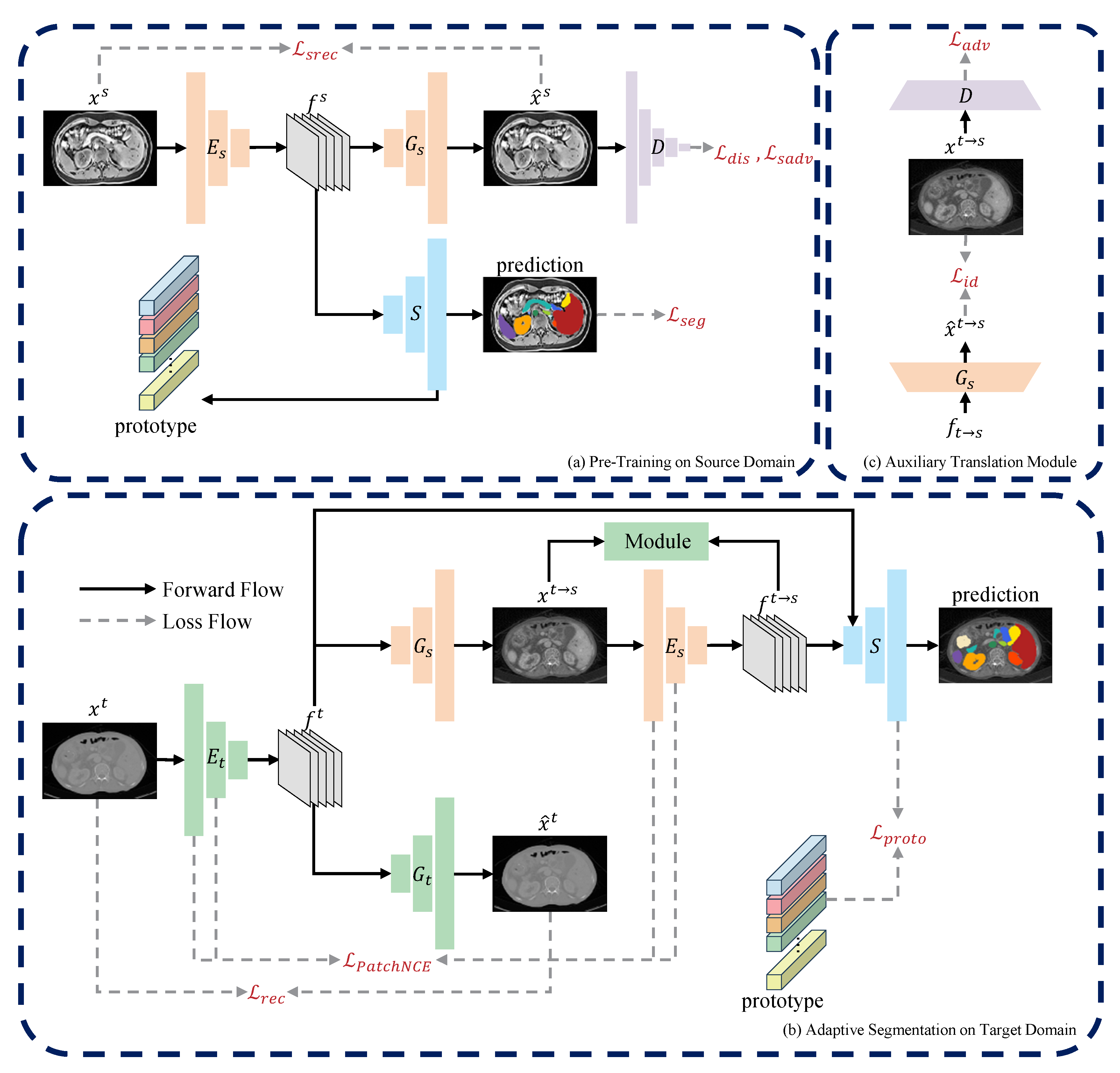
3.1. Overview
3.2. Pre-Training on Source Domain
3.3. Domain-Adaptive Segmentation
3.3.1. Source-Free One-Way Image Translation
3.3.2. Auxiliary Translation Module
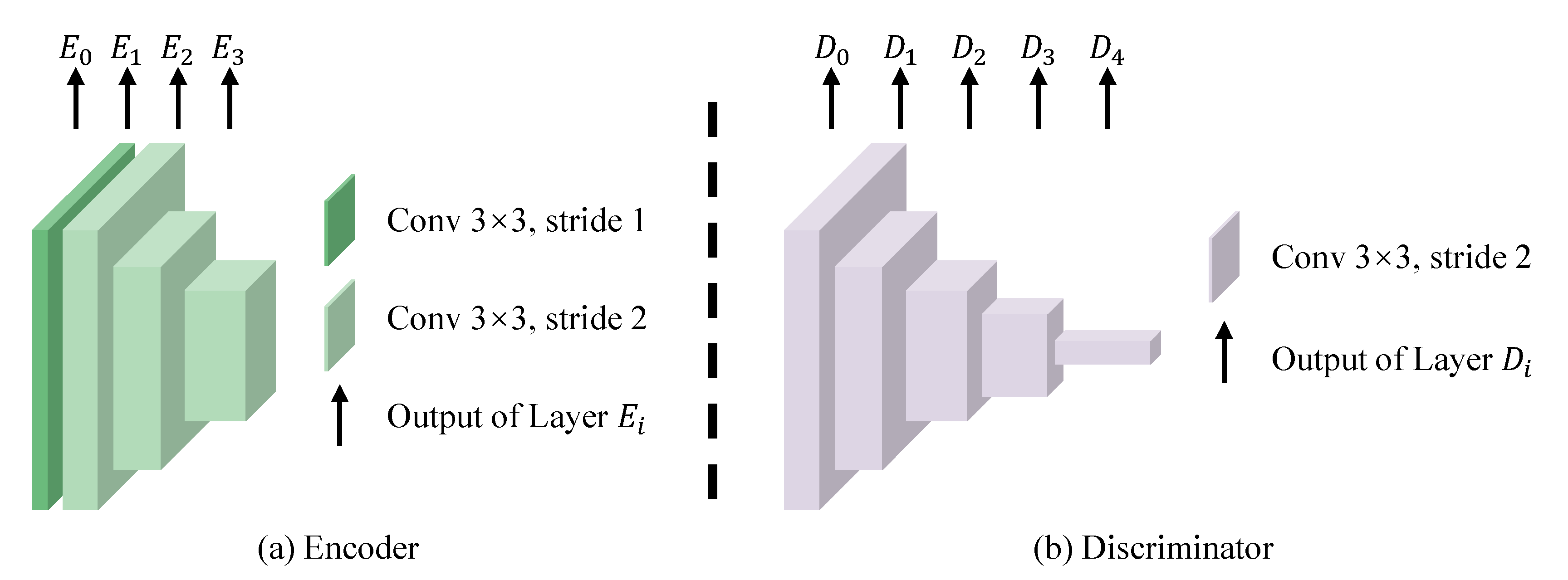
3.4. Network Architecture
3.5. Training Detail
4. Experiments
4.1. Experimental Settings
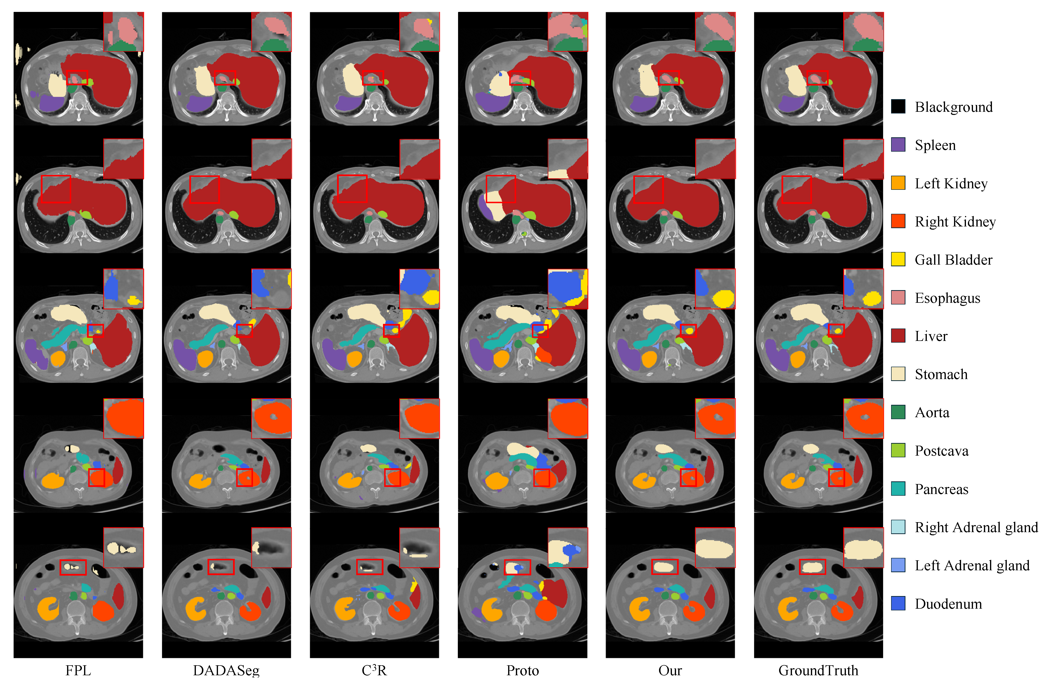
4.2. Quantitative and Qualitative Results
4.3. Model Analysis
4.3.1. Ablation Study
4.3.2. Impact of One-Way Image Translation
4.3.3. Impact of Auxiliary Translation Module
4.3.4. Model Convergence Analysis
5. Conclusions and Discussion
Author Contributions
Funding
Institutional Review Board Statement
Informed Consent Statement
Data Availability Statement
Conflicts of Interest
References
- Wang, R.; Lei, T.; Cui, R.; Zhang, B.; Meng, H.; Nandi, A.K. Medical image segmentation using deep learning: A survey. IET Image Process. 2022, 16, 1243–1267. [Google Scholar] [CrossRef]
- Alirr, O.I.; Rahni, A.A.A. Survey on liver tumour resection planning system: Steps, techniques, and parameters. J. Digit. Imaging 2020, 33, 304–323. [Google Scholar] [CrossRef] [PubMed]
- Chen, X.; Pang, Y.; Yap, P.T.; Lian, J. Multi-scale anatomical regularization for domain-adaptive segmentation of pelvic CBCT images. Med. Phys. 2024, 51, 8804–8813. [Google Scholar] [CrossRef]
- Dou, Q.; Ouyang, C.; Chen, C.; Chen, H.; Heng, P.A. Unsupervised Cross-Modality Domain Adaptation of ConvNets for Biomedical Image Segmentations with Adversarial Loss. arXiv 2018, arXiv:1804.10916. [Google Scholar]
- Xian, J.; Li, X.L.; Tu, D.; Zhu, S.; Zhang, C.; Liu, X.; Li, X.; Yang, X. Unsupervised Cross-Modality Adaptation via Dual Structural-Oriented Guidance for 3D Medical Image Segmentation. IEEE Trans. Med. Imaging 2023, 42, 1774–1785. [Google Scholar] [CrossRef]
- Ganin, Y.; Lempitsky, V. Unsupervised domain adaptation by backpropagation. In Proceedings of the 32nd International Conference on International Conference on Machine Learning ICML’15, Lille, France, 6–11 July 2015; Volume 37, pp. 1180–1189. [Google Scholar] [CrossRef]
- Liang, J.; Hu, D.; Feng, J. Do We Really Need to Access the Source Data? Source Hypothesis Transfer for Unsupervised Domain Adaptation. In Proceedings of the International Conference on Machine Learning, Virtual, 13–18 July 2020. [Google Scholar]
- Liu, Y.; Zhang, W.; Wang, J. Source-Free Domain Adaptation for Semantic Segmentation. In Proceedings of the IEEE/CVF Conference on Computer Vision and Pattern Recognition (CVPR), Nashville, TN, USA, 20–25 June 2021; pp. 1215–1224. [Google Scholar] [CrossRef]
- Stan, S.; Rostami, M. Unsupervised model adaptation for source-free segmentation of medical images. Med. Image Anal. 2024, 95, 103179. [Google Scholar] [CrossRef]
- Bateson, M.; Kervadec, H.; Dolz, J.; Lombaert, H.; Ben Ayed, I. Source-free domain adaptation for image segmentation. Med. Image Anal. 2022, 82, 102617. [Google Scholar] [CrossRef]
- Wu, J.; Wang, G.; Gu, R.; Lu, T.; Chen, Y.; Zhu, W.; Vercauteren, T.; Ourselin, S.; Zhang, S. UPL-SFDA: Uncertainty-Aware Pseudo Label Guided Source-Free Domain Adaptation for Medical Image Segmentation. IEEE Trans. Med. Imaging 2023, 42, 3932–3943. [Google Scholar] [CrossRef]
- Yang, C.; Guo, X.; Chen, Z.; Yuan, Y. Source free domain adaptation for medical image segmentation with fourier style mining. Med. Image Anal. 2022, 79, 102457. [Google Scholar] [CrossRef]
- Chen, C.; Liu, Q.; Jin, Y.; Dou, Q.; Heng, P.A. Source-Free Domain Adaptive Fundus Image Segmentation with Denoised Pseudo-Labeling. In Proceedings of the Medical Image Computing and Computer Assisted Intervention—MICCAI, Strasbourg, France, 27 September–1 October 2021; pp. 225–235. [Google Scholar] [CrossRef]
- Huai, Z.; Ding, X.; Li, Y.; Li, X. Context-Aware Pseudo-label Refinement for Source-Free Domain Adaptive Fundus Image Segmentation. In Proceedings of the Medical Image Computing and Computer Assisted Intervention—MICCAI, Vancouver, BC, Canada, 8–12 October 2023; pp. 618–628. [Google Scholar] [CrossRef]
- Jiang, J.; Hu, Y.C.; Tyagi, N.; Rimner, A.; Lee, N.; Deasy, J.O.; Berry, S.; Veeraraghavan, H. PSIGAN: Joint Probabilistic Segmentation and Image Distribution Matching for Unpaired Cross-Modality Adaptation-Based MRI Segmentation. IEEE Trans. Med. Imaging 2020, 39, 4071–4084. [Google Scholar] [CrossRef]
- Chen, X.; Lian, C.; Wang, L.; Deng, H.; Kuang, T.; Fung, S.; Gateno, J.; Yap, P.T.; Xia, J.J.; Shen, D. Anatomy-Regularized Representation Learning for Cross-Modality Medical Image Segmentation. IEEE Trans. Med. Imaging 2021, 40, 274–285. [Google Scholar] [CrossRef] [PubMed]
- Liu, H.; Zhuang, Y.; Song, E.; Xu, X.; Hung, C.C. A bidirectional multilayer contrastive adaptation network with anatomical structure preservation for unpaired cross-modality medical image segmentation. Comput. Biol. Med. 2022, 149, 105964. [Google Scholar] [CrossRef] [PubMed]
- Wu, J.; Guo, D.; Wang, G.; Yue, Q.; Yu, H.; Li, K.; Zhang, S. FPL+: Filtered Pseudo Label-Based Unsupervised Cross-Modality Adaptation for 3D Medical Image Segmentation. IEEE Trans. Med. Imaging 2024, 43, 3098–3109. [Google Scholar] [CrossRef] [PubMed]
- Wu, F.; Zhuang, X. Unsupervised Domain Adaptation With Variational Approximation for Cardiac Segmentation. IEEE Trans. Med. Imaging 2021, 40, 3555–3567. [Google Scholar] [CrossRef]
- Chen, C.; Dou, Q.; Chen, H.; Qin, J.; Heng, P.A. Synergistic Image and Feature Adaptation: Towards Cross-Modality Domain Adaptation for Medical Image Segmentation. Proc. AAAI Conf. Artif. Intell. 2019, 33, 865–872. [Google Scholar] [CrossRef]
- Dou, Q.; Ouyang, C.; Chen, C.; Chen, H.; Glocker, B.; Zhuang, X.; Heng, P.A. PnP-AdaNet: Plug-and-Play Adversarial Domain Adaptation Network at Unpaired Cross-Modality Cardiac Segmentation. IEEE Access 2019, 7, 99065–99076. [Google Scholar] [CrossRef]
- Chen, X.; Kuang, T.; Deng, H.; Fung, S.H.; Gateno, J.; Xia, J.J.; Yap, P.T. Dual Adversarial Attention Mechanism for Unsupervised Domain Adaptive Medical Image Segmentation. IEEE Trans. Med. Imaging 2022, 41, 3445–3453. [Google Scholar] [CrossRef]
- Sun, Y.; Dai, D.; Xu, S. Rethinking adversarial domain adaptation: Orthogonal decomposition for unsupervised domain adaptation in medical image segmentation. Med. Image Anal. 2022, 82, 102623. [Google Scholar] [CrossRef]
- Ding, S.; Liu, Z.; Liu, P.; Zhu, W.; Xu, H.; Li, Z.; Niu, H.; Cheng, J.; Liu, T. C3R: Category contrastive adaptation and consistency regularization for cross-modality medical image segmentation. Expert Syst. Appl. 2025, 269, 126304. [Google Scholar] [CrossRef]
- Hong, J.; Zhang, Y.D.; Chen, W. Source-free unsupervised domain adaptation for cross-modality abdominal multi-organ segmentation. Knowl.-Based Syst. 2022, 250, 109155. [Google Scholar] [CrossRef]
- Yu, Q.; Xi, N.; Yuan, J.; Zhou, Z.; Dang, K.; Ding, X. Source-Free Domain Adaptation for Medical Image Segmentation via Prototype-Anchored Feature Alignment and Contrastive Learning. In Proceedings of the Medical Image Computing and Computer Assisted Intervention—MICCAI, Vancouver, BC, Canada, 8–12 October 2023; pp. 3–12. [Google Scholar] [CrossRef]
- Park, T.; Efros, A.A.; Zhang, R.; Zhu, J.Y. Contrastive Learning for Unpaired Image-to-Image Translation. In Proceedings of the Computer Vision—ECCV, Glasgow, UK, 23–28 August 2020; pp. 319–345. [Google Scholar] [CrossRef]
- He, K.; Zhang, X.; Ren, S.; Sun, J. Identity Mappings in Deep Residual Networks. In Proceedings of the Computer Vision—ECCV, Amsterdam, The Netherlands, 11–14 October 2016; pp. 630–645. [Google Scholar] [CrossRef]
- Wu, Y.; He, K. Group Normalization. In Proceedings of the European Conference on Computer Vision (ECCV), Munich, Germany, 8–14 September 2018. [Google Scholar]
- Ramachandran, P.; Zoph, B.; Le, Q.V. Searching for Activation Functions. arXiv 2017, arXiv:1710.05941. [Google Scholar]
- Maas, A.L.; Hannun, A.Y.; Ng, A.Y. Rectifier nonlinearities improve neural network acoustic models. In Proceedings of the International Conference on Machine Learning, Atlanta, GA, USA, 17–19 June 2013; Volume 30, p. 3. [Google Scholar]
- Loshchilov, I.; Hutter, F. Decoupled Weight Decay Regularization. In Proceedings of the International Conference on Learning Representations, New Orleans, LA, USA, 6–9 May 2019. [Google Scholar]
- Tanwisuth, K.; Fan, X.; Zheng, H.; Zhang, S.; Zhang, H.; Chen, B.; Zhou, M. A Prototype-Oriented Framework for Unsupervised Domain Adaptation. In Proceedings of the Advances in Neural Information Processing Systems, Online, 6–14 December 2021; Curran Associates, Inc.: Red Hook, NY, USA, 2021; Volume 34, pp. 17194–17208. [Google Scholar]
- Ji, Y.; Bai, H.; Yang, J.; Ge, C.; Zhu, Y.; Zhang, R.; Li, Z.; Zhang, L.; Ma, W.; Wan, X.; et al. AMOS: A Large-Scale Abdominal Multi-Organ Benchmark for Versatile Medical Image Segmentation. arXiv 2022, arXiv:2206.08023. [Google Scholar]


| Symbol | Meaning |
|---|---|
| Image sets of source and target modalities | |
| Annotation set corresponding to | |
| f | Encoder-extracted image features |
| Source and target encoders | |
| Source and target generators | |
| D | Image discriminator |
| S | Segmenter |
| Modality | Training Set | Validation Set | Test Set |
|---|---|---|---|
| Source domain (MRI) | 40 | 20 | − |
| Target domain (CT) | 200 | 20 | 80 |
| Dice (%) ↑ | FPL [18] | DADAseg [22] | C3R [24] | AOS [25] | Proto [26] | UPL [11] | Ours |
|---|---|---|---|---|---|---|---|
| Spleen | 61.09 ± 25.16 ** | 85.30 ± 11.87 | 70.22 ± 18.72 ** | 2.46 ± 1.06 ** | 60.55 ± 17.82 ** | 13.18 ± 6.44 ** | 86.86 ± 10.62 |
| Right kidney | 74.59 ± 18.45 ** | 72.15 ± 13.09 ** | 77.71 ± 13.17 | 1.40 ± 0.39 ** | 56.25 ± 25.67 ** | - | 81.85 ± 22.41 |
| Left kidney | 72.72 ± 24.32 ** | 82.82 ± 16.18 | 75.84 ± 12.84 | 1.04 ± 0.33 ** | 59.35 ± 23.36 ** | 0.02 ± 0.10 ** | 79.22 ± 22.47 |
| Gall bladder | 35.44 ± 28.87 ** | 31.65 ± 18.63 ** | 29.81 ± 23.18 ** | 0.34 ± 0.31 ** | 15.53 ± 14.29 ** | - | 50.25 ± 31.20 |
| Esophagus | 25.74 ± 21.23 ** | 45.20 ± 24.27 ** | 49.02 ± 21.66 ** | 0.13 ± 0.09 ** | 26.94 ± 17.40 ** | - | 57.70 ± 24.36 |
| Liver | 80.89 ± 9.80 ** | 92.44 ± 5.57 | 82.58 ± 10.58 ** | 6.21 ± 0.64 ** | 77.00 ± 10.82 ** | 42.23 ± 9.70 ** | 88.58 ± 8.98 |
| Stomach | 34.82 ± 23.93 ** | 53.98 ± 28.90 ** | 58.20 ± 21.35 | 2.64 ± 1.18 ** | 39.63 ± 15.97 ** | 6.86 ± 6.11 ** | 58.96 ± 22.47 |
| Aorta | 62.84 ± 22.91 ** | 86.45 ± 8.92 | 78.12 ± 8.26 ** | 1.12 ± 0.45 ** | 68.76 ± 22.85 ** | 8.63 ± 4.09 ** | 82.59 ± 14.18 |
| Postcava | 56.03 ± 14.94 ** | 75.12 ± 11.60 | 64.46 ± 12.21 | 1.00 ± 0.28 ** | 46.40 ± 17.26 ** | - | 63.28 ± 16.34 |
| Pancreas | 45.20 ± 21.44 ** | 59.26 ± 18.73 | 57.50 ± 15.67 | 0.80 ± 0.23 ** | 30.94 ± 19.05 ** | - | 50.17 ± 19.20 |
| Right adrenal gland | 36.97 ± 18.67 | 29.41 ± 15.86 ** | 31.67 ± 10.35 ** | 0.04 ± 0.02 ** | 17.02 ± 14.99 ** | - | 40.35 ± 21.08 |
| Left adrenal gland | 33.24 ± 22.10 | 19.94 ± 17.85 ** | 17.11 ± 12.59 ** | 0.05 ± 0.02 ** | 16.55 ± 13.79 ** | - | 34.13 ± 24.89 |
| Duodenum | 26.89 ± 16.14 ** | 44.31 ± 19.69 | 40.60 ± 14.53 ** | 0.60 ± 0.23 ** | 17.92 ± 11.81 ** | - | 45.17 ± 18.97 |
| Avg | 49.73 ± 13.34 ** | 59.85 ± 8.91 ** | 56.37 ± 9.06 ** | 1.37 ± 0.19 ** | 40.99 ± 12.61 ** | 5.46 ± 1.14 ** | 63.01 ± 12.61 |
| ASSD (mm) ↓ | FPL [18] | DADAseg [22] | C3R [24] | AOS [25] | Proto [26] | UPL [11] | Ours |
|---|---|---|---|---|---|---|---|
| Spleen | 14.35 ± 12.73 ** | 6.07 ± 2.62 ** | 20.95 ± 16.92 ** | 54.09 ± 4.25 ** | 12.96 ± 5.65 ** | 35.72 ± 5.67 ** | 4.78 ± 5.21 |
| Right kidney | 13.36 ± 10.07 ** | 26.66 ± 5.79 ** | 5.40 ± 3.39 ** | 54.58 ± 8.32 ** | 17.06 ± 14.54 ** | - | 3.72 ± 4.09 |
| Left kidney | 6.96 ± 7.77 | 7.41 ± 3.75 | 5.57 ± 4.08 | 63.10 ± 5.87 ** | 11.37 ± 9.82 ** | 70.36 ± 9.43 ** | 6.23 ± 6.82 |
| Gall bladder | 15.13 ± 23.19 | 28.09 ± 7.01 ** | 27.36 ± 17.96 ** | 54.09 ± 18.64 ** | 30.55 ± 17.37 ** | - | 8.47 ± 19.83 |
| Esophagus | 6.51 ± 5.99 | 6.96 ± 5.74 * | 3.98 ± 3.40 | 63.33 ± 5.06 ** | 30.76 ± 14.09 ** | - | 5.09 ± 5.15 |
| Liver | 12.27 ± 5.86 ** | 3.51 ± 2.90 | 10.41 ± 7.57 ** | 31.36 ± 3.80 ** | 11.16 ± 7.10 ** | 26.41 ± 5.53 ** | 6.47 ± 4.73 |
| Stomach | 30.64 ± 16.10 ** | 8.31 ± 6.98 | 15.44 ± 10.45 ** | 41.02 ± 7.04 ** | 15.37 ± 6.13 ** | 45.33 ± 10.31 ** | 10.12 ± 4.62 |
| Aorta | 5.30 ± 5.00 | 3.31 ± 1.25 | 3.12 ± 2.88 | 46.31 ± 1.98 ** | 5.58 ± 6.42 * | 24.56 ± 3.45 ** | 4.24 ± 3.64 |
| Postcava | 5.32 ± 3.47 | 3.53 ± 1.86 | 3.99 ± 3.03 | 47.16 ± 1.12 ** | 9.58 ± 4.33 ** | - | 5.87 ± 3.16 |
| Pancreas | 8.86 ± 7.25 | 7.19 ± 6.35 | 6.26 ± 4.34 | 45.05 ± 4.94 ** | 15.01 ± 8.97 ** | - | 11.67 ± 5.19 |
| Right adrenal gland | 4.92 ± 5.22 | 12.10 ± 4.79 * | 9.23 ± 7.49 | 61.88 ± 2.67 ** | 17.63 ± 8.23 ** | - | 7.45 ± 19.90 |
| Left adrenal gland | 7.45 ± 10.91 | 14.83 ± 7.31 ** | 15.34 ± 7.44 ** | 61.29 ± 3.16 ** | 40.38 ± 14.97 ** | - | 6.49 ± 8.07 |
| Duodenum | 12.85 ± 11.08 * | 6.76 ± 7.13 | 8.69 ± 6.11 | 49.04 ± 8.67 ** | 20.02 ± 9.23 ** | - | 9.22 ± 7.65 |
| Avg | 11.23 ± 4.87 ** | 10.35 ± 2.22 ** | 10.44 ± 4.25 ** | 51.71 ± 2.90 ** | 18.26 ± 6.39 ** | 39.62 ± 4.71 ** | 6.94 ± 4.12 |
| Variant | Dice (%) ↑ | ASSD (mm) ↓ |
|---|---|---|
| Without | 28.14 ± 11.22 | 20.33 ± 9.19 |
| Without | 61.55 ± 13.95 | 8.11 ± 5.87 |
| Without | 56.94 ± 15.18 | 9.04 ± 5.87 |
| Without | 61.38 ± 13.87 | 7.67 ± 5.39 |
| Ours | 63.01 ± 12.61 | 6.94 ± 4.12 |
| Variant | Dice (%) ↑ | ASSD (mm) ↓ |
|---|---|---|
| 16 patches | 38.57 ± 15.47 | 13.25 ± 6.67 |
| 32 patches | 61.87 ± 12.82 | 7.00 ± 4.39 |
| 64 patches | 63.01 ± 12.61 | 6.94 ± 4.12 |
| 128 patches | 59.56 ± 14.67 | 8.81 ± 5.70 |
| 256 patches | 55.63 ± 16.13 | 10.09 ± 6.80 |
| Variant | Dice (%) ↑ | ASSD (mm) ↓ |
|---|---|---|
| 59.42 ± 14.10 | 8.41 ± 5.25 | |
| 59.94 ± 14.32 | 8.58 ± 5.57 | |
| 63.01 ± 12.61 | 6.94 ± 4.12 | |
| 61.72 ± 13.93 | 7.51 ± 5.44 |
| Variant | Dice (%) ↑ | ASSD (mm) ↓ |
|---|---|---|
| 24.52 ± 15.33 | 27.89 ± 13.84 | |
| 41.70 ± 17.71 | 16.30 ± 9.68 | |
| 54.00 ± 16.84 | 10.46 ± 6.88 | |
| 58.94 ± 14.89 | 8.47 ± 5.73 | |
| 59.94 ± 14.49 | 8.38 ± 5.77 | |
| 63.01 ± 12.61 | 6.94 ± 4.12 | |
| 60.26 ± 14.11 | 8.37 ± 5.74 | |
| 61.20 ± 14.04 | 7.76 ± 5.80 | |
| 57.11 ± 15.24 | 9.72 ± 6.50 |
Disclaimer/Publisher’s Note: The statements, opinions and data contained in all publications are solely those of the individual author(s) and contributor(s) and not of MDPI and/or the editor(s). MDPI and/or the editor(s) disclaim responsibility for any injury to people or property resulting from any ideas, methods, instructions or products referred to in the content. |
© 2025 by the authors. Licensee MDPI, Basel, Switzerland. This article is an open access article distributed under the terms and conditions of the Creative Commons Attribution (CC BY) license (https://creativecommons.org/licenses/by/4.0/).
Share and Cite
Zhang, X.; Chen, X.; Wang, Y.; Liu, D.; Hong, Y. Source-Free Domain Adaptation for Cross-Modality Abdominal Multi-Organ Segmentation Challenges. Information 2025, 16, 460. https://doi.org/10.3390/info16060460
Zhang X, Chen X, Wang Y, Liu D, Hong Y. Source-Free Domain Adaptation for Cross-Modality Abdominal Multi-Organ Segmentation Challenges. Information. 2025; 16(6):460. https://doi.org/10.3390/info16060460
Chicago/Turabian StyleZhang, Xiyu, Xu Chen, Yang Wang, Dongliang Liu, and Yifeng Hong. 2025. "Source-Free Domain Adaptation for Cross-Modality Abdominal Multi-Organ Segmentation Challenges" Information 16, no. 6: 460. https://doi.org/10.3390/info16060460
APA StyleZhang, X., Chen, X., Wang, Y., Liu, D., & Hong, Y. (2025). Source-Free Domain Adaptation for Cross-Modality Abdominal Multi-Organ Segmentation Challenges. Information, 16(6), 460. https://doi.org/10.3390/info16060460