

GC-MT: A Novel Vessel Trajectory Sequence Prediction Method for Marine Regions


Abstract
1. Introduction
- (1)
- This paper presents the GC-MT model, an innovative approach for intelligent spatiotemporal vessel trajectory prediction that operates without the need for an attention mechanism. By integrating GCN with the Mamba model, it effectively captures the motion characteristics, temporal features, and interaction relationships among moving vessels, thereby facilitating efficient sequence modeling and accurate forecasting of future trajectories.
- (2)
- Extensive experiments conducted on AIS data demonstrate that the proposed prediction method significantly outperforms other baseline approaches in terms of accuracy, underscoring its potential applicability in long-term and complex maritime environments.
- (3)
- Given the intricacies of real-world AIS data, this study incorporates feasibility analysis into existing preprocessing techniques to enhance the overall efficiency of the vessel trajectory prediction methodology.
2. Materials and Methods
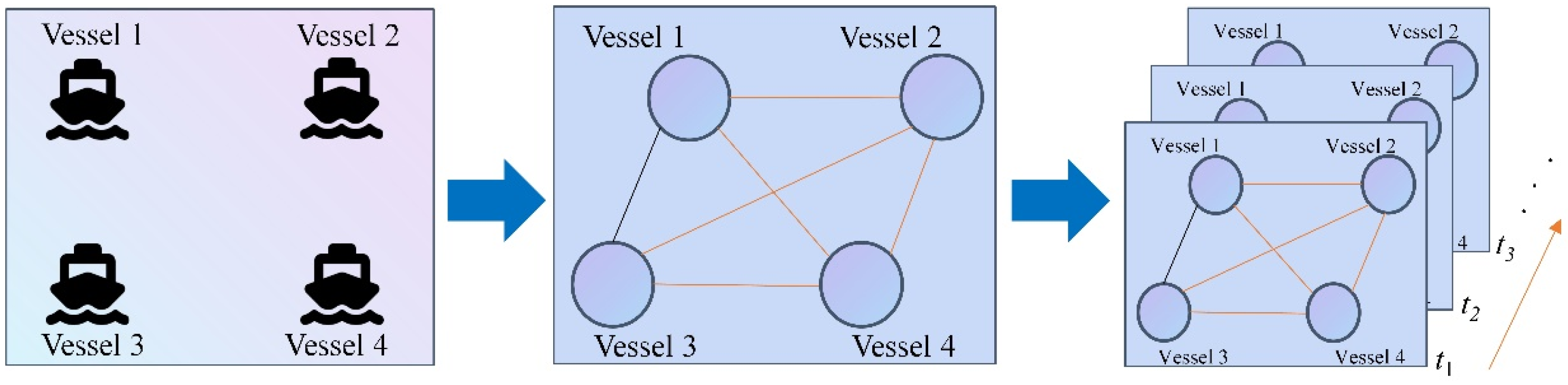
2.1. Problem Explanation
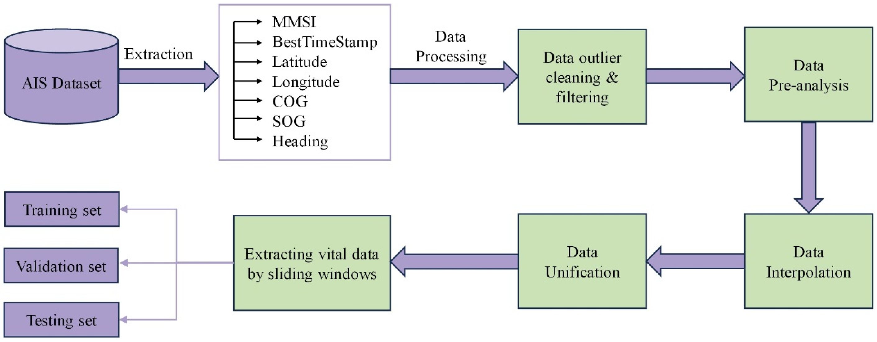
2.2. Data Preprocessing
2.2.1. Data Cleaning and Filtering
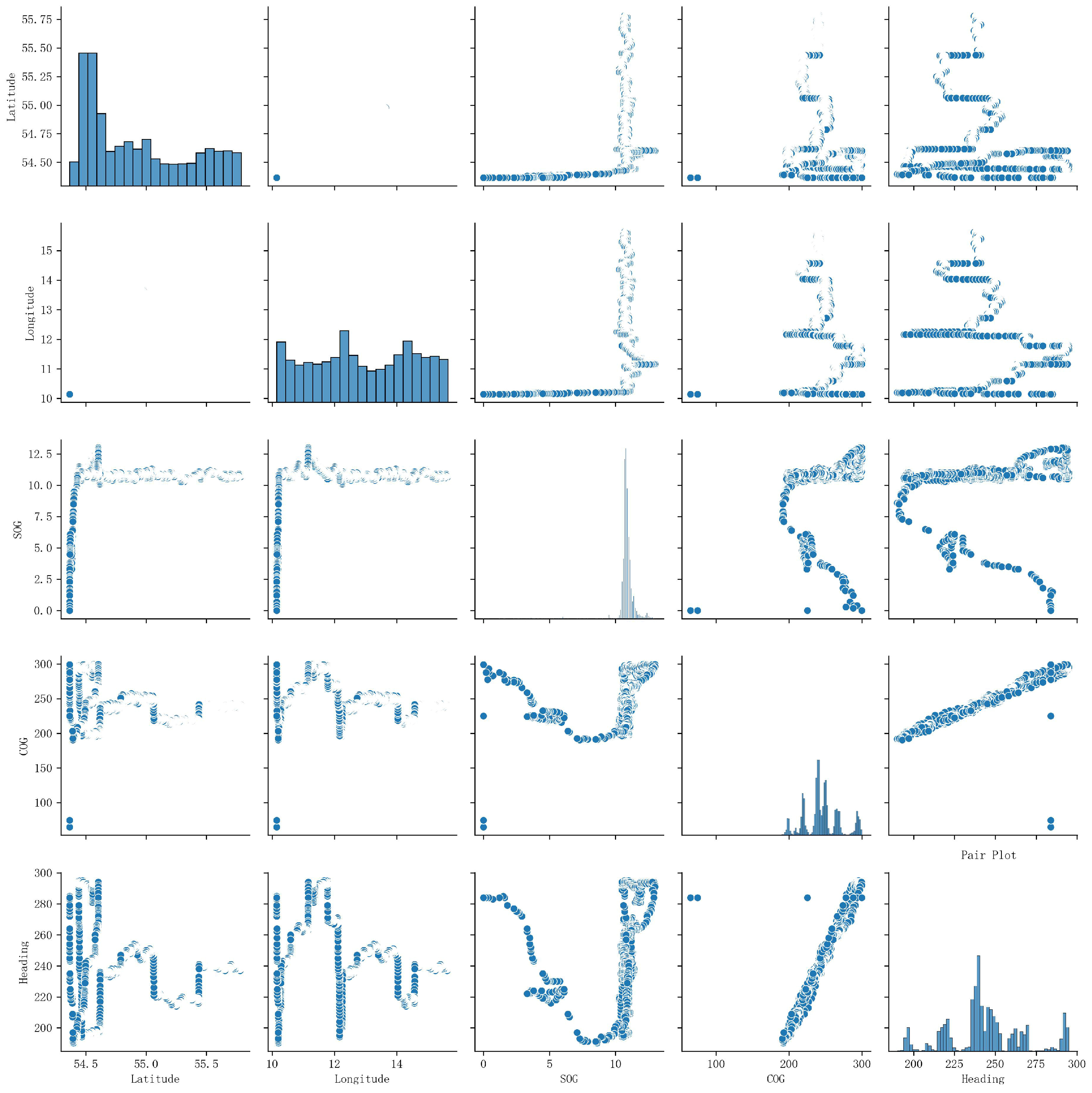
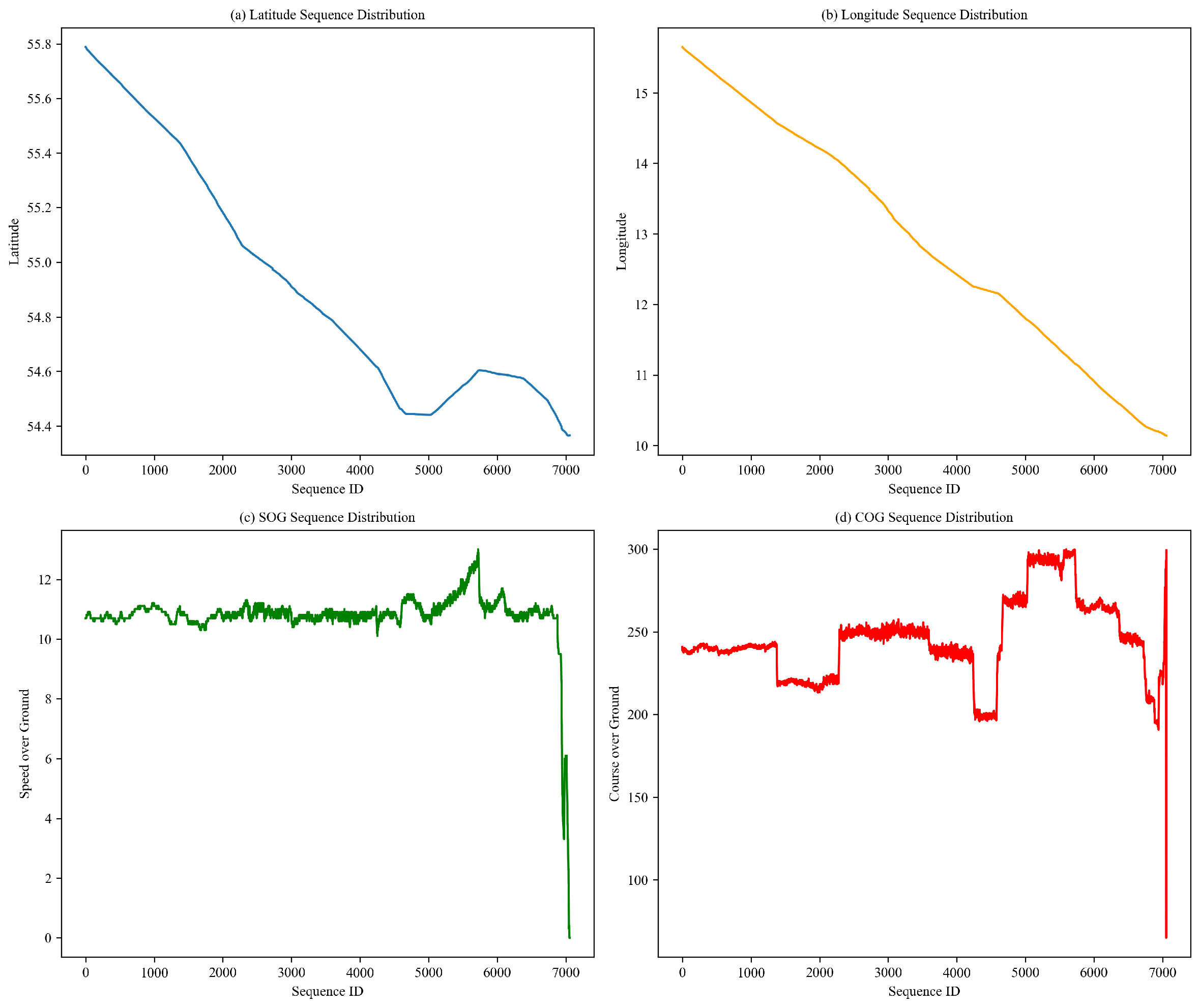
2.2.2. Data Pre-Analysis
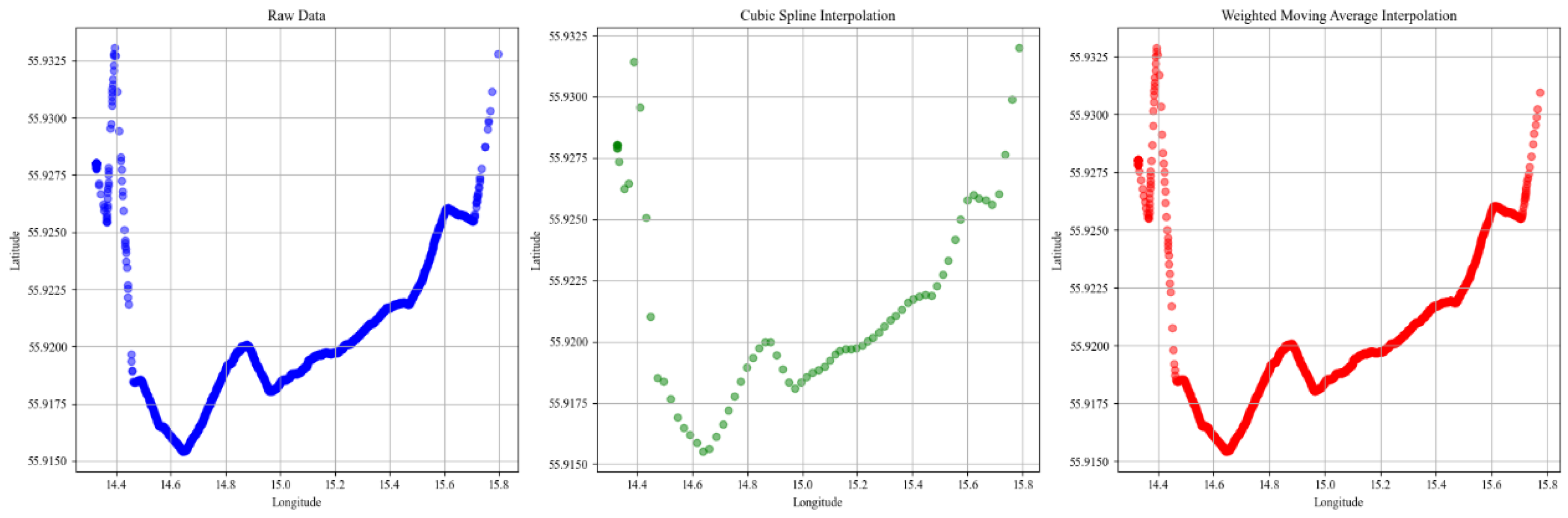
2.2.3. Data Interpolation
2.2.4. Data Standardization
2.2.5. Sampling Data by Sliding Windows
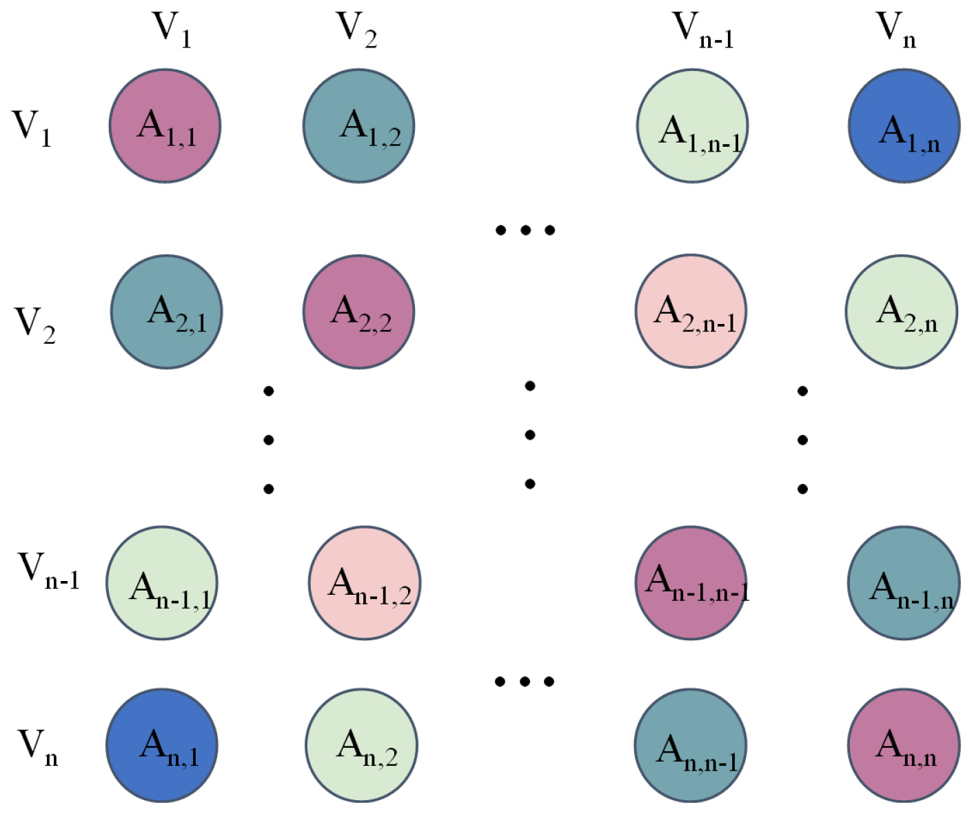
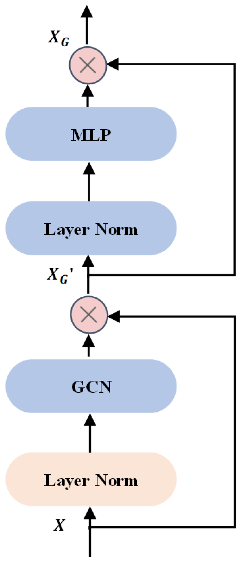
2.3. GCN Module
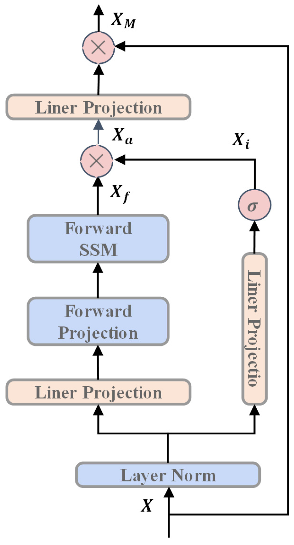
2.4. Mamba Module
2.5. End-to-End Learning
2.6. Overall Architecture
3. Results
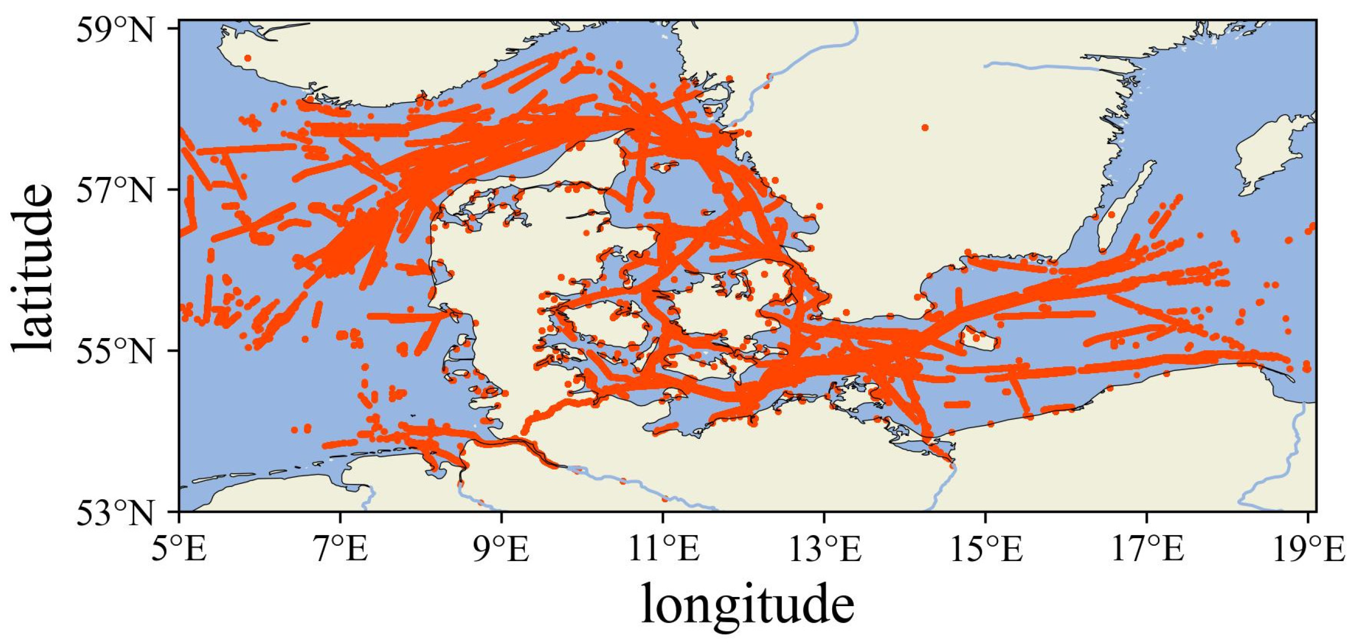
3.1. Dataset
3.2. Evaluation Metrics
3.3. Comparison Baselines
3.4. Environment and Hyperparameters
3.5. Results and Analysis
4. Discussion
5. Conclusions
Author Contributions
Funding
Institutional Review Board Statement
Informed Consent Statement
Data Availability Statement
Conflicts of Interest
Abbreviations
| AIS | Automatic Identification System |
| GCN | Graph Convolutional Network |
| MNN | Mamba Neural Network |
| GC-MT | Graph Convolutional Mamba Network |
| SSM | State Space Model |
| SSSM | Selective State Space Model |
| LTI | Linear Time-Invariant |
| RNN | Recurrent Neural Network |
| LSTM | Long Short-Term Memory |
| GRU | Gated Recurrent Unit |
| ADE | Average Displacement Error |
| FDE | Final Displacement Error |
References
- Ma, D.; Ma, W.; Hao, S.; Jin, S.; Qu, F. Ship’s Response to Low-Sulfur Regulations: From the Perspective of Route, Speed and Refueling Strategy. Comput. Ind. Eng. 2021, 155, 107140. [Google Scholar] [CrossRef]
- Guo, S.; Mou, J.; Chen, L.; Chen, P. An Anomaly Detection Method for AIS Trajectory Based on Kinematic Interpolation. J. Mar. Sci. Eng. 2021, 9, 609. [Google Scholar] [CrossRef]
- Liu, H.; Liu, Y.; Li, B.; Qi, Z. Ship Abnormal Behavior Detection Method Based on Optimized GRU Network. J. Mar. Sci. Eng. 2022, 10, 249. [Google Scholar] [CrossRef]
- Fossen, S.; Fossen, T.I. Extended Kalman Filter Design and Motion Prediction of Ships Using Live Automatic Identification System (Ais) Data. In Proceedings of the 2018 2nd European Conference on Electrical Engineering and Computer Science (EECS), Bern, Switzerland, 20–22 December 2018; IEEE: New York, NY, USA, 2018; pp. 464–470. [Google Scholar]
- Jaskólski, K. Automatic Identification System (AIS) Dynamic Data Estimation Based on Discrete Kalman Filter (KF) Algorithm. Zesz. Nauk. Akad. Mar. Wojennej 2017, 58, 71–87. [Google Scholar] [CrossRef]
- Zhang, X.; Liu, G.; Hu, C.; Ma, X. Wavelet Analysis Based Hidden Markov Model for Large Ship Trajectory Prediction. In Proceedings of the 2019 Chinese Control Conference (CCC), Guangzhou, China, 27–30 July 2019; IEEE: New York, NY, USA, 2019; pp. 2913–2918. [Google Scholar]
- Luo, X.; Wang, J.; Li, J.; Lu, H.; Lai, Q.; Zhu, X. Research on Ship Trajectory Prediction Using Extended Kalman Filter and Least-Squares Support Vector Regression Based on AIS Data. In Proceedings of the 2021 6th International Conference on Intelligent Transportation Engineering (ICITE 2021): Beijing, China, 29–31 October; Springer Nature: Singapore, 2022; pp. 1123–1131. [Google Scholar]
- Rong, H.; Teixeira, A.P.; Soares, C.G. Ship Trajectory Uncertainty Prediction Based on a Gaussian Process Model. Ocean. Eng. 2019, 182, 499–511. [Google Scholar] [CrossRef]
- Alam, M.M.; Spadon, G.; Etemad, M.; Torgo, L.; Milios, E. Enhancing Short-Term Vessel Trajectory Prediction with Clustering for Heterogeneous and Multi-Modal Movement Patterns. Ocean. Eng. 2024, 308, 118303. [Google Scholar] [CrossRef]
- Guo, S.; Liu, C.; Guo, Z.; Feng, Y.; Hong, F.; Huang, H. Trajectory Prediction for Ocean Vessels Base on K-Order Multivariate Markov Chain. In Wireless Algorithms, Systems, and Applications, Proceedings of the 13th International Conference, WASA 2018, Tianjin, China, 20–22 June 2018; Springer International Publishing: Berlin/Heidelberg, Germany, 2018; pp. 140–150. [Google Scholar]
- Xiaopeng, T.; Xu, C.; Lingzhi, S.; Zhe, M.; Qing, W. Vessel Trajectory Prediction in Curving Channel of Inland River. In Proceedings of the 2015 International Conference on Transportation Information and Safety (ICTIS), Wuhan, China, 25–28 June 2015; IEEE: New York, NY, USA, 2015; pp. 706–714. [Google Scholar]
- Zhang, M.; Huang, L.; Wen, Y.; Zhang, J.; Huang, Y.; Zhu, M. Short-Term Trajectory Prediction of Maritime Vessel Using k-Nearest Neighbor Points. J. Mar. Sci. Eng. 2022, 10, 1939. [Google Scholar] [CrossRef]
- Ma, H.; Zuo, Y.; Li, T. Vessel Navigation Behavior Analysis and Multiple-Trajectory Prediction Model Based on AIS Data. J. Adv. Transp. 2022, 2022, 6622862. [Google Scholar] [CrossRef]
- Capobianco, S.; Millefiori, L.M.; Forti, N.; Braca, P.; Willett, P. Deep Learning Methods for Vessel Trajectory Prediction Based on Recurrent Neural Networks. IEEE Trans. Aerosp. Electron. Syst. 2021, 57, 4329–4346. [Google Scholar] [CrossRef]
- Zhang, Z.; Ni, G.; Xu, Y. Ship Trajectory Prediction Based on LSTM Neural Network. In Proceedings of the 2020 IEEE 5th Information Technology and Mechatronics Engineering Conference (ITOEC), Chongqing, China, 12–14 June 2020; IEEE: New York, NY, USA, 2020; pp. 1356–1364. [Google Scholar]
- Forti, N.; Millefiori, L.M.; Braca, P.; Willett, P. Prediction Oof Vessel Trajectories from AIS Data via Sequence-to-Sequence Recurrent Neural Networks. In Proceedings of the ICASSP 2020—2020 IEEE International Conference on Acoustics, Speech and Signal Processing (ICASSP), Barcelona, Spain, 4–8 May 2020; IEEE: New York, NY, USA, 2020; pp. 8936–8940. [Google Scholar]
- Suo, Y.; Chen, W.; Claramunt, C.; Yang, S. A Ship Trajectory Prediction Framework Based on a Recurrent Neural Network. Sensors 2020, 20, 5133. [Google Scholar] [CrossRef]
- Zhang, X.; Fu, X.; Xiao, Z.; Xu, H.; Qin, Z. Vessel Trajectory Prediction in Maritime Transportation: Current Approaches and Beyond. IEEE Trans. Intell. Transp. Syst. 2022, 23, 19980–19998. [Google Scholar] [CrossRef]
- Xue, H.; Wang, S.; Xia, M.; Guo, S. G-Trans: A Hierarchical Approach to Vessel Trajectory Prediction with GRU-Based Transformer. Ocean. Eng. 2024, 300, 117431. [Google Scholar] [CrossRef]
- Donandt, K.; Söffker, D. Incorporating Navigation Context into Inland Vessel Trajectory Prediction: A Gaussian Mixture Model and Transformer Approach. In Proceedings of the 2024 27th International Conference on Information Fusion (FUSION), Venice, Italy, 7–11 July 2024; IEEE: New York, NY, USA, 2024; pp. 1–8. [Google Scholar]
- Murray, B.; Perera, L.P. Ship Behavior Prediction via Trajectory Extraction-Based Clustering for Maritime Situation Awareness. J. Ocean. Eng. Sci. 2022, 7, 1–13. [Google Scholar] [CrossRef]
- Kipf, T.N.; Welling, M. Semi-supervised classification with graph convolutional networks. arXiv 2016, arXiv:1609.02907. [Google Scholar]
- Wu, L.; Sun, P.; Hong, R.; Fu, Y.; Wang, X.; Wang, M. SocialGCN: An Efficient Graph Convolutional Network Based Model for Social Recommendation. arXiv 2018, arXiv:1811.02815. [Google Scholar]
- Zhao, L.; Song, Y.; Zhang, C.; Liu, Y.; Wang, P.; Lin, T.; Deng, M.; Li, H. T-GCN: A Temporal Graph Convolutional Network for Traffic Prediction. IEEE Trans. Intell. Transp. Syst. 2019, 21, 3848–3858. [Google Scholar] [CrossRef]
- Voelker, A.R.; Eliasmith, C. Improving Spiking Dynamical Networks: Accurate Delays, Higher-Order Synapses, and Time Cells. Neural Comput. 2018, 30, 569–609. [Google Scholar] [CrossRef]
- Gu, A.; Dao, T. Mamba: Linear-Time Sequence Modeling with Selective State Spaces 2024. arXiv 2023, arXiv:2312.00752. [Google Scholar]
- Agarap, A.F. Deep Learning Using Rectified Linear Units (ReLU) 2019. arXiv 2018, arXiv:1803.08375. [Google Scholar]
- Iserles, A. A First Course in the Numerical Analysis of Differential Equations; Cambridge University Press: Cambridge, UK, 2009. [Google Scholar]
- Hendrycks, D.; Gimpel, K. Gaussian Error Linear Units (GELUs) 2023. arXiv 2016, arXiv:1606.08415. [Google Scholar]
- Pellegrini, S.; Ess, A.; Schindler, K.; Van Gool, L. You’ll Never Walk Alone: Modeling Social Behavior for Multi-Target Tracking. In Proceedings of the 2009 IEEE 12th international conference on computer vision, Kyoto, Japan, 27 September–4 October 2009; IEEE: New York, NY, USA, 2009; pp. 261–268. [Google Scholar]
- Alahi, A.; Goel, K.; Ramanathan, V.; Robicquet, A.; Fei-Fei, L.; Savarese, S. Social Lstm: Human Trajectory Prediction in Crowded Spaces. In Proceedings of the IEEE Conference on Computer Vision and Pattern Recognition, Las Vegas, NV, USA, 26 June–1 July 2016; pp. 961–971. [Google Scholar]
- Adege, A.B.; Lin, H.-P.; Wang, L.-C. Mobility Predictions for IoT Devices Using Gated Recurrent Unit Network. IEEE Internet Things J. 2019, 7, 505–517. [Google Scholar] [CrossRef]
- Mohamed, A.; Qian, K.; Elhoseiny, M.; Claudel, C. Social-Stgcnn: A Social Spatio-Temporal Graph Convolutional Neural Network for Human Trajectory Prediction. In Proceedings of the IEEE/CVF Conference on Computer Vision and Pattern Recognition, Seattle, WA, USA, 13–19 June 2020; pp. 14424–14432. [Google Scholar]
- Loshchilov, I.; Hutter, F. Decoupled Weight Decay Regularization. arXiv 2019, arXiv:1711.05101. [Google Scholar]


| Water | Time Period | Vessel Quantity | SOG (NM/h) | Boundary | |
|---|---|---|---|---|---|
| Longitude (°) | Latitude (°) | ||||
| Danish | November 2022 | 4438 | [1.0 kt, 51.2 kt] | [0.5°W, 21° E] | [53.56° N, 59.55° N] |
| Mexico | March 2022 | 5556 | [1.0 kt, 22.0 kt] | [21°W, 31° W] | [−95° S, 83° S] |
| Baseline | Danish | Mexico | ||
|---|---|---|---|---|
| ADE | FDE | ADE | FDE | |
| LSTM | 0.6412 | 0.9800 | 0.7365 | 0.9384 |
| GRU | 0.6236 | 0.9681 | 0.6470 | 0.9622 |
| Seq2seq | 0.5226 | 0.7661 | 0.5286 | 0.8374 |
| STGCNN | 0.3512 | 0.4877 | 0.3552 | 0.5331 |
| GC-MT | 0.2281 | 0.3316 | 0.2557 | 0.3998 |
| Impro (%) | 35% | 32% | 28% | 25% |
| Prediction Length | Danish | Mexico | ||
|---|---|---|---|---|
| ADE | FDE | ADE | FDE | |
| 10 | 0.2836 | 0.4055 | 0.3112 | 0.4998 |
| 30 | 0.3106 | 0.4263 | 0.3274 | 0.5398 |
| 60 | 0.3785 | 0.5286 | 0.3536 | 0.5614 |
Disclaimer/Publisher’s Note: The statements, opinions and data contained in all publications are solely those of the individual author(s) and contributor(s) and not of MDPI and/or the editor(s). MDPI and/or the editor(s) disclaim responsibility for any injury to people or property resulting from any ideas, methods, instructions or products referred to in the content. |
© 2025 by the authors. Licensee MDPI, Basel, Switzerland. This article is an open access article distributed under the terms and conditions of the Creative Commons Attribution (CC BY) license (https://creativecommons.org/licenses/by/4.0/).
Share and Cite
Ye, H.; Wang, W.; Zhang, X. GC-MT: A Novel Vessel Trajectory Sequence Prediction Method for Marine Regions. Information 2025, 16, 311. https://doi.org/10.3390/info16040311
Ye H, Wang W, Zhang X. GC-MT: A Novel Vessel Trajectory Sequence Prediction Method for Marine Regions. Information. 2025; 16(4):311. https://doi.org/10.3390/info16040311
Chicago/Turabian StyleYe, Haixiong, Wei Wang, and Xiliang Zhang. 2025. "GC-MT: A Novel Vessel Trajectory Sequence Prediction Method for Marine Regions" Information 16, no. 4: 311. https://doi.org/10.3390/info16040311
APA StyleYe, H., Wang, W., & Zhang, X. (2025). GC-MT: A Novel Vessel Trajectory Sequence Prediction Method for Marine Regions. Information, 16(4), 311. https://doi.org/10.3390/info16040311