Predictions from Generative Artificial Intelligence Models: Towards a New Benchmark in Forecasting Practice

Abstract

This paper aims to determine whether there is a case for promoting a new benchmark for forecasting practice via the innovative application of generative artificial intelligence (Gen-AI) for predicting the future. Today, forecasts can be generated via Gen-AI models without the need for an in-depth understanding of forecasting theory, practice, or coding. Therefore, using three datasets, we present a comparative analysis of forecasts from Gen-AI models against forecasts from seven univariate and automated models from the forecast package in R, covering both parametric and non-parametric forecasting techniques. In some cases, we find statistically significant evidence to conclude that forecasts from Gen-AI models can outperform forecasts from popular benchmarks like seasonal ARIMA, seasonal naïve, exponential smoothing, and Theta forecasts (to name a few). Our findings also indicate that the accuracy of forecasts from Gen-AI models can vary not only based on the underlying data structure but also on the quality of prompt engineering (thus highlighting the continued importance of forecasting education), with the forecast accuracy appearing to improve at longer horizons. Therefore, we find some evidence towards promoting forecasts from Gen-AI models as benchmarks in future forecasting practice. However, at present, users are cautioned against reliability issues and Gen-AI being a black box in some cases.

1. Introduction

OpenAI succeeded in making artificial intelligence (AI) accessible to the world (n.b., it is only available to the population with access to the internet) and has demonstrated how generative AI (Gen-AI), a subset of deep learning, can transform our lives [1]. As a result, since its launch in November 2022, the natural language model Chat Generative Pre-trained Transformer (ChatGPT) continues to disrupt industries across the globe [2], with other models like Microsoft Copilot and Google’s Gemini emerging since.

Given its popularity as the first to market, researchers have already delved into many aspects of ChatGPT, from its potential impact on education [3] and research [4] to its impact on various fields ranging from marketing [5] to forensics [6], to name a few. However, the rapid adoption of Gen-AI is also highlighting its many shortcomings, which range from hallucinations [7] to bias and ethical issues [8] and to the negative environmental impact [9,10]. Furthermore, concerns about AI making certain job functions obsolete are also rapidly emerging [11]. Therefore, the importance of promoting the use of AI for intelligence augmentation, i.e., enhancing human intelligence and improving the efficiency of human tasks as opposed to being a replacement, is crucial [12]. In this regard, recent experimental evidence points towards an opportunity for using Gen-AI to reduce productivity inequalities [13].

A few months after ChatGPT was launched, Hassani and Silva [14] discussed the potential impact of Gen-AI on data science and related intelligence augmentation. Building on that work, here, we focus our attention on “forecasting”, which is a common data science task that helps with capacity planning, goal setting, and anomaly detection [15]. Today, Gen-AI tools offer the capability for non-experts to generate forecasts and use these in their decision-making processes. Nvidia’s CEO Jensen Huang recently predicted the death of coding in a world where “the programming language is human, [and] everybody in the world is now a programmer” [16].

In a world where humans can now generate forecasts without an in-depth knowledge or understanding of forecasting theory, practice, or coding, we are motivated to determine whether there is a need to rethink forecasting practice concerning the benchmarks that are used to evaluate forecasting models. Benchmark forecasts are meant to have significant levels of accuracy and be simple to generate with minimal computational effort. It is an important aspect of forecasting practice as investments in new forecasting models should only be entertained if there is sufficient evidence of a proposed model significantly outperforming popular benchmarks. As outlined in [17], when proposing a new forecasting model or undertaking forecast evaluations for univariate time series, it is important to consider the naïve, seasonal naïve, or ARIMA model as a benchmark for comparing forecast accuracy. The random walk (i.e., the naïve range of models) is known to be a tough benchmark to outperform [18]. Exponential smoothing, Holt–Winters and Theta forecasts are also identified as benchmark methods in one of the most comprehensive reviews of forecasting theory and practice [18].

Recent research confirms the superiority of AI models across various computational tasks by building on theories of deep learning, scalability, and efficiency [19,20]. As discussed, and evidenced below, these computational tasks now include forecasting using historical data. Given that large language models can generate forecasts based on AI prompts, this study is grounded by the following research question:

RQ: 

Should forecasts from Gen-AI models (for example, forecasts from ChatGPT or Microsoft Copilot) be considered a new benchmark in forecasting practice?

To the best of our knowledge, there exists no published academic work that seeks to propose or evaluate forecasts from Gen-AI models as a benchmark or contender in the field of forecasting. In contrast, machine learning models have been applied and compared with statistical models for time series forecasting [21], whilst deep learning models have also received much attention in the recent past [22]. Some studies propose hybrid forecasting models that combine machine learning, decomposition techniques, and statistical models and compare the performance against benchmarks like ARIMA [23]. Therefore, it is evident that studies seeking to introduce benchmarks via comparative analysis of models are important. For example, in relation to machine learning, Gu et al. [24] sought to introduce a new set of benchmarks for the predictive accuracy of machine learning methods via a comparative analysis, whilst Zhou et al. [25] presented a comparison of deep learning models for equity premium forecasting. Gen-AI models, given their reliance on deep learning, can extract and transform features from data and identify hidden nonlinear relations without the need to rely on econometric assumptions and human expertise [25].

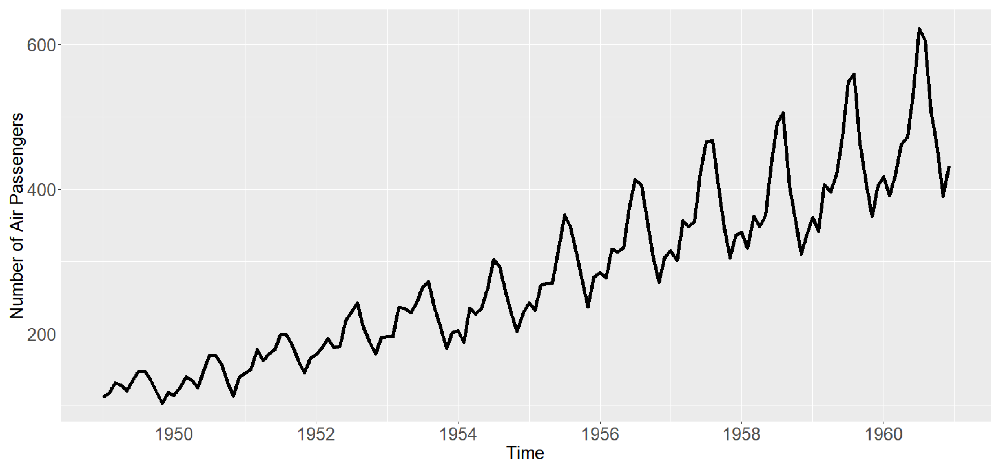
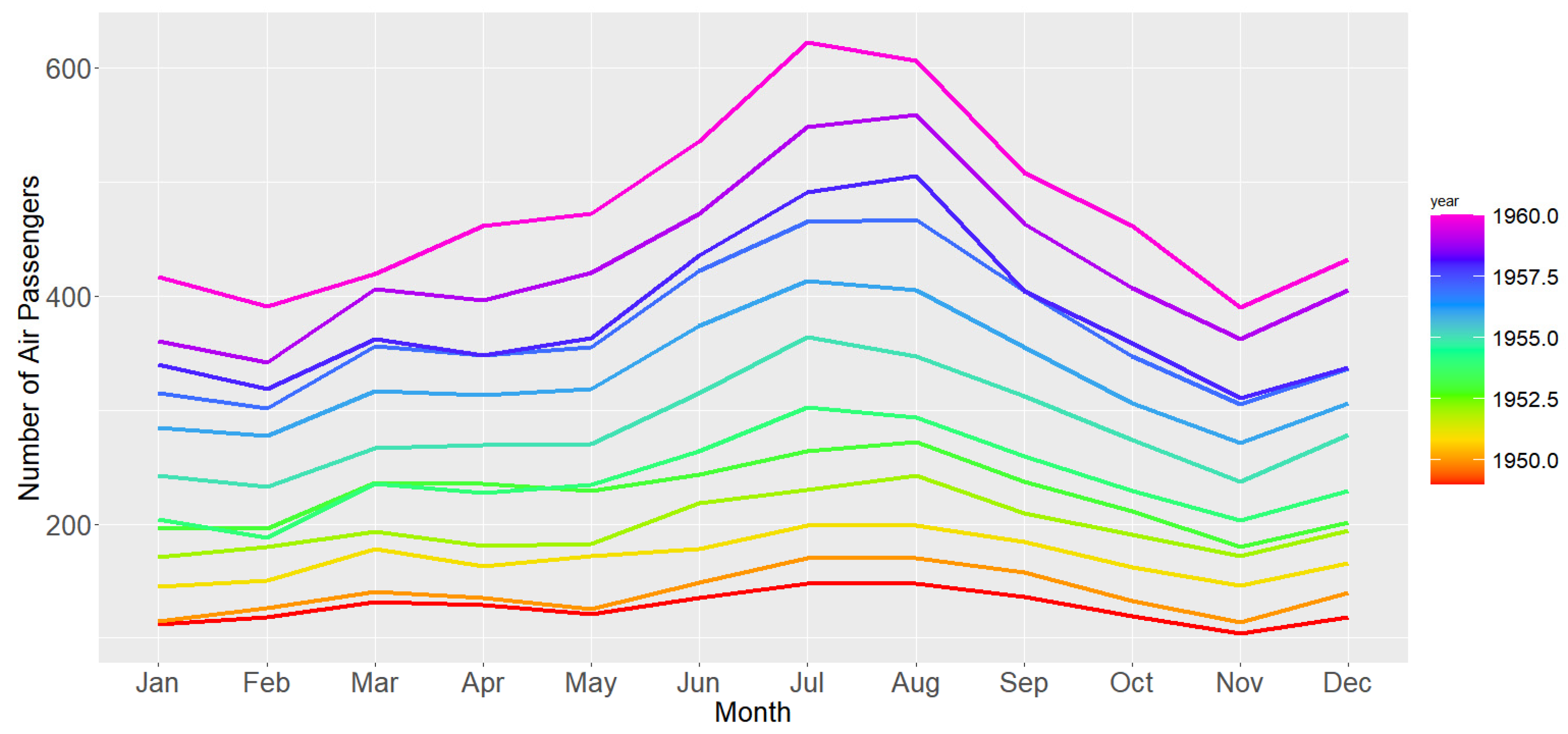
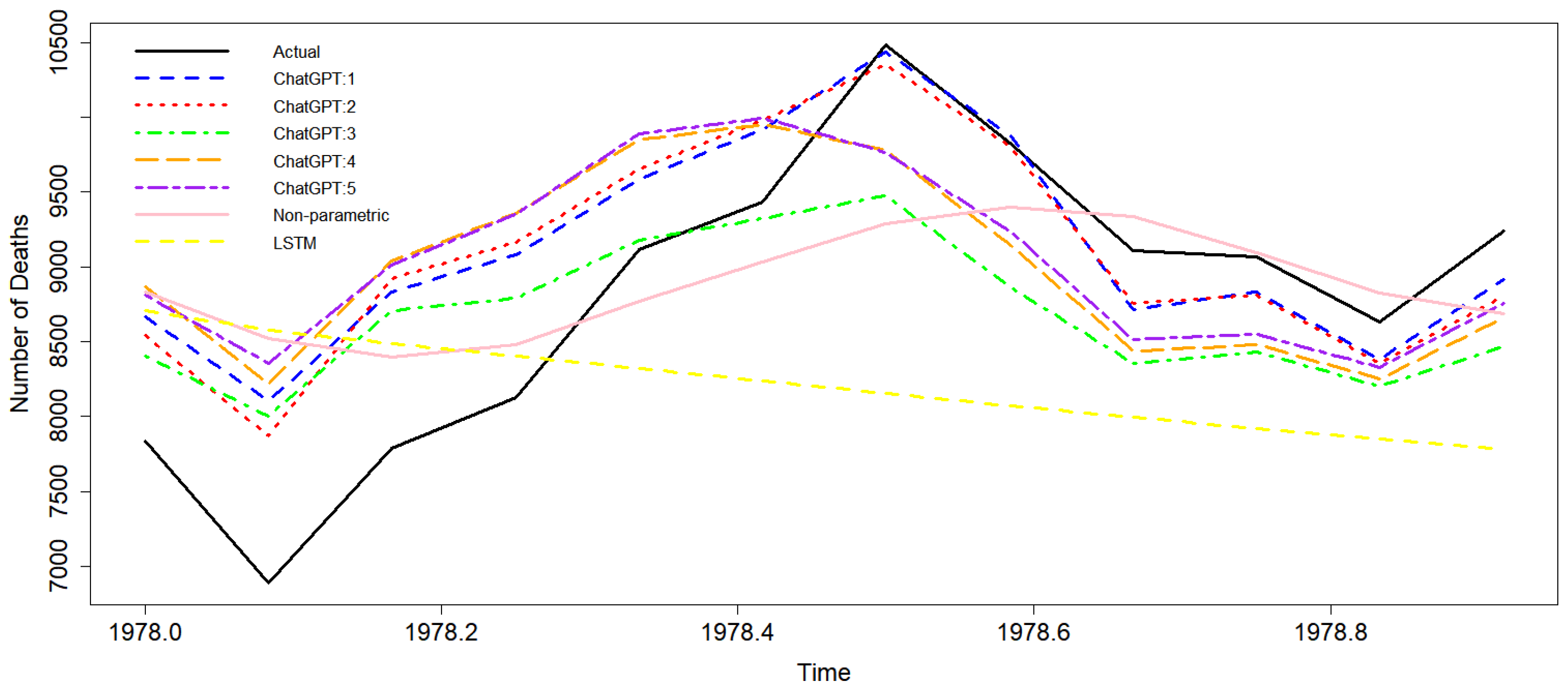
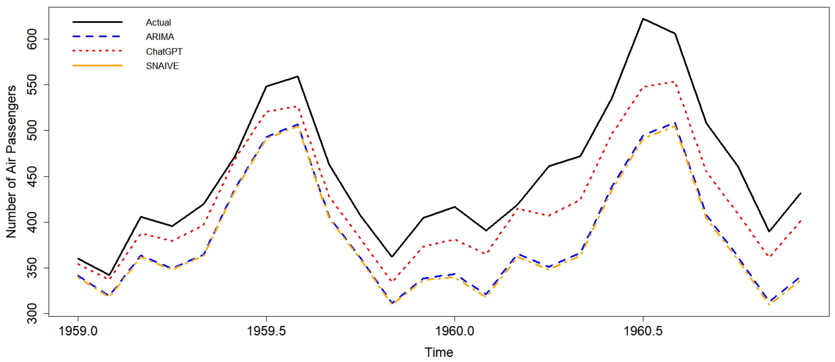
Therefore, our interest lies in conducting a comparative analysis of forecasts from Gen-AI models in comparison to forecasts generated by established, traditional benchmark forecasting models to determine whether there is sufficient evidence to promote a new benchmark model for forecasting practice in the age of Gen-AI. In this paper, initially, we consider ChatGPT as an example of a Gen-AI tool and use it to forecast three time series, as an example. These include the U.S. accidental death series [26,27,28], the air passengers series [29] and UK tourist arrivals [30,31]. The forecasts from ChatGPT are compared with seven forecasting models which represent both parametric and non-parametric forecasting techniques and are provided via the forecast package in R [32]. These include seasonal naïve (SNAIVE), Holt–Winters (HW), autoregressive integrated moving average (ARIMA), exponential smoothing (ETS), trigonometric seasonality, Box–Cox transformation, ARMA errors, trend and seasonal components (TBATS), seasonal–trend decomposition using LOESS (STL), and the Theta method. Models such as SNAIVE, ARIMA, ETS, Theta, and HW are identified as benchmark forecasting models in [17,18], whilst the rest have the shared properties of being automated, simple, and applicable with minimum computational effort without the need for an in-depth understanding of forecasting theory. However, unlike with Gen-AI models, the application of these selected benchmarks will require some basic coding skills and an understanding of the use of the programming language R.

Through the empirical analysis, we find that in some cases, forecasts from Gen-AI models can significantly outperform forecasts from popular benchmarks. Therefore, we find evidence for promoting the use of Gen-AI models as benchmarks in future forecast evaluations. However, our findings also indicate that the accuracy of these forecasts could vary depending on the underlying data structures, the level of forecasting knowledge, and education, which will invariably influence the quality of prompt engineering and the training data underlying the Gen-AI model (e.g., paid vs. free versions). Reliability-related issues are also prevalent, alongside Gen-AI models being black boxes and thus restricting interpretability of the models being used.

Through our research, we make several contributions to forecasting practice and the literature. First, we present the most comprehensive evaluation of forecasts from Gen-AI models to date, comparing them to seven traditional benchmark methods. Second, based on our findings, we can propose the use of Gen-AI models as benchmark forecasting models for forecast evaluations. In doing so, we add to the list of historical benchmark forecasting models in [18], which tend to require basic programming and coding skills. Third, our research also seeks to educate and improve the basic forecasting capabilities of the public by sharing the coding used to generate competing forecasts via the forecast package in R. Finally, through the discussion, we also seek to improve the public understanding and capability of engaging with Gen-AI models for forecasting; we share the prompts used on Microsoft Copilot that resulted in a forecast for one of the datasets.

The remainder of this paper is organized such that Section 2 briefly introduces the forecasting models with the codes used to generate the forecasts, Section 3 presents the forecasting results and analysis, a discussion follows in Section 4, and the paper concludes in Section 5.

2. Methods and Data

In this section, we present the benchmark forecasting models, the data, and the metrics used to evaluate forecasts. The forecasts from Gen-AI models were generated by prompting ChatGPT (GPT-4), unless mentioned otherwise. It is noteworthy that we do not attempt to define the models that are generated by ChatGPT as these were not known in advance of the application.

2.1. Benchmark Forecasting Models

All forecasts were generated using the forecast package in R (v.4.3.1) [32]. To minimize replication of information already in the public domain, we present concise summaries of each model and the code used to generate the benchmark forecasts to enable replication.

2.1.1. Holt–Winters (HW)

Forecasts from the Holt–Winters model [33,34] were generated via the forecast package in R using the following code.

install.packages(“forecast”)

library(forecast)

data<-scan()

time_series<-ts(data,start=c(1973,1), frequency=12)

model<-HoltWinters(time_series,h=12)

Where the data object only scans the training data, which in the case of the death series, is from January 1973 to December 1977.

2.1.2. Autoregressive Integrated Moving Average (ARIMA)

The ARIMA model is one of the most established and widely used time series forecasting models [35].

The modeling process seeks to separate the signal and noise by adopting past observations and taking into consideration the degree of differencing, autoregressive, and moving average components. The “auto.arima” model from the forecast package in R begins by repeating KPSS tests to determine the number of differences d. The data are then differenced d times to minimize the Akaike information criterion (AIC), and the values of p (number of autoregressive terms) and q (number of lagged forecast errors in the forecasting equation) are obtained. The algorithm is efficient as instead of considering every possible combination of p and q, it traverses the model space via a stepwise search. Thereafter, the “current model” is determined by searching the four ARIMA models, namely, ARIMA(2,d,2), ARIMA(0,d,0), ARIMA(1,d,0), and ARIMA(0,d,1), for the one which minimizes the AIC. If d = 0, then the constant c is included; if d ≥ 1, then the constant c is set to zero. The model also evaluates variations on the current model by varying p and q by ± 1 and including/excluding c. The steps following the minimization of the AIC are repeated until no lower AIC can be found. Those interested in the theory underlying this model are referred to [35].

library(forecast)

data<-scan()

time_series<-ts(data,start=c(1973,1), frequency=12)

model<-auto.arima(time_series,h=12)

2.1.3. Exponential Smoothing (ETS)

The theory underlying the ETS model is explained in [35]. In brief, the ETS model evaluates over 30 possible options and considers the error, trend, and seasonal components in choosing the best exponential smoothing model by optimizing initial values and parameters using maximum likelihood estimation and selecting the best model based on the Akaike information criterion [35].

library(forecast)

data<-scan()

time_series<-ts(data,start=c(1973,1), frequency=12)

model<-ets(time_series,h=12)

2.1.4. Trigonometric Seasonality, Box–Cox Transformation, ARMA Errors, Trend and Seasonal Components (TBATS)

The TBATS model is aimed at providing accurate forecasts for time series with complex seasonality. A detailed description of the TBATS model can be found in [36]. We consider this as a benchmark given its simple application, like the other models considered here, which makes it easily accessible at minimal cost.

library(forecast)

data<-scan()

time_series<-ts(data,start=c(1973,1), frequency=12)

model<-tbats(time_series,h=12)

2.1.5. Seasonal Naïve (SNAIVE)

SNAIVE is a popular benchmark model for forecasting seasonal time series data. This model returns forecasts from an ARIMA(0,0,0)(0,1,0)m model, where m is the seasonal period (m=12 in the case of our data). In the most basic terms, this model considers the historical value from the previous season to be the best forecast for this season.

library(forecast)

data<-scan()

time_series<-ts(data,start=c(1973,1), frequency=12)

model<-snaive(time_series,h=12)

2.1.6. Seasonal–Trend Decomposition Using LOESS (STL)

The theory underlying the STL model can be found in [35], where the authors describe this model as a robust decomposition method which uses loess for estimating non-linear relationships. This algorithm works by decomposing the time series using STL before forecasting the seasonally adjusted series and returning the reseasonalized forecasts. Once more, we use this as a benchmark given its straightforward application to any time series.

library(forecast)

data<-scan()

time_series<-ts(data,start=c(1973,1), frequency=12)

model<-stlf(time_series,h=12)

2.1.7. Theta Forecast

The final benchmark model considered in this paper is the Theta method [37], which can be described as simple exponential smoothing with drift. The series is seasonally adjusted (in the case of seasonal time series) using a classical multiplicative decomposition before the Theta method is applied. The resulting forecasts are then reseasonalized. Those interested in an alternative explanation of the theory underlying this method are referred to [38].

library(forecast)

data<-scan()

time_series<-ts(data,start=c(1973,1), frequency=12)

model<-thetaf(time_series,h=12)

Following the approach taken in [39], the forecast evaluation not only relies on the root mean squared error (RMSE) and mean absolute percentage error (MAPE) as loss functions but also the mean absolute error (MAE), as in [23]. MAPE values less than 10% are indicative of highly accurate forecasting, 10–20% are indicative of good forecasting, and 20–50% are indicative of reasonable forecasting, whilst 50% or more indicate inaccurate forecasting [40].

2.2. Data

Below we present and summarize the two main datasets used in this paper and refer readers to recent publications that summarize the dataset introduced in the discussion section.

2.2.1. Death Series

The main analysis considers the popular monthly U.S. accidental death series from January 1973 to December 1977 [26,27,28]. Figure 1 shows the death series. As is visible, it is affected by seasonal variations and a slowly decreasing trend that appears to gradually increase over time.

Table 1. Summary statistics for the death series.

Mean	SD	Median	IQR	Normality	CV	Breakpoints
8788	958	8729	1234	p = 0.44	0.11	1973(10)

Note: SD, standard deviation; IQR, interquartile range; CV, coefficient of variation. Normality reports the p-value from a Shapiro–Wilk test for normality. The breakpoints are calculated using the Bai and Perron [41] test.

presents some summary statistics which describe the data. The Shapiro–Wilk test for normality is not statistically significant, thereby confirming that the series is normally distributed. During the observed period, deaths averaged 8788 per month in the U.S. The Bai and Perron [41] test for breakpoints indicates that the series was affected by a structural break in October 1973. The coefficient of variation (CV) indicates that the variation in the death series can be quantified as 11%. Figure 2 presents a seasonal plot for the death series. As visible, this shows that deaths peaked annually in July.

2.2.2. Air Passengers Series

The air passengers series [29] records monthly total U.S. air passengers from 1949 to 1960 (Figure 3) and has a different structure to the death Series. Here, there is an upward-sloping trend and seasonality which increases over time. The seasonal plot (Figure 4) indicates that most air passengers were recorded annually in July. The descriptive statistics in

Table 2. Summary statistics for the air passengers series.

Mean	SD	Median	IQR	Normality	CV	Breakpoints
280	120	266	181	p < 0.01	0.43	1951(2) 1953(2) 1955(5) 1957(2) 1959(3)

Note: SD, standard deviation; IQR, interquartile range, CV: coefficient of variation. Normality reports the p-value from a Shapiro–Wilk test for normality. The breakpoints are calculated using the Bai and Perron [41] test.

further evidence the differences between the two datasets being used. The Shapiro–Wilk test for normality is statistically significant and thereby indicates that the time series is not normally distributed. This indicates that the median air passengers value of 266 is a more appropriate measure of central tendency for this data. The Bai and Perron [41] breakpoints test concludes that five breakpoints are impacting this time series, and the CV of 43% confirms that this series reports more variation than the death series (CV = 11%).

3. Results

3.1. Application: Death Series

At the initial stage, our intention is not to determine whether one forecasting model is significantly better than a competing forecasting model. Instead, our quest is modest in that we are seeking to identify whether there is a case for promoting the use of forecasts from Gen-AI models (i.e., ChatGPT in this example) as a benchmark forecasting model in the future.

To evaluate this proposition, we set up a forecasting exercise whereby observations from January 1973 up until December 1977 were set aside for training our models. We then generated a h = 12-months-ahead forecast over the test period from January 1978 to December 1978. The findings are presented below.

First and foremost, we were able to prompt ChatGPT into producing forecasts for this dataset from seven different models that included ARIMA, seasonal ARIMA (SARIMA), a non-parametric model, and a long short-term memory (LSTM) model. It is important to note that these models are not defined in Section 2 because we could not foresee which models Gen-AI would rely on. Furthermore, the key point of this research is to determine whether forecasts from Gen-AI, regardless of which forecasting model it might be using, should be considered as a benchmark model in future forecasting studies. Figure 5 shows the forecasts from these various ChatGPT-based models plotted against the actual data so that readers can visualize and compare the loss functions reported in

Table 3. Out-of-sample forecasting results for the death series.

Error	ChatGPT: 1	ChatGPT: 2	ChatGPT: 3	ChatGPT: 4	ChatGPT: 5	Non-Parametric	LSTM
RMSE	645.78	637.53	738.96	862.3	857.77	731.67	1292.11
MAPE	6.51%	6.53%	7.76%	9.60%	9.41%	6.94%	13.26%
MAE	526.00	534.67	666	807.33	786.83	579.08	1175.42

Note: All forecasts listed above were generated via ChatGPT. Shown in bold font is the model reporting the lowest forecast error based on a given loss function.

. One clear message from Figure 5 is that the LSTM model generated by ChatGPT is performing very poorly at forecasting the death series.

Table 3 presents the forecast errors for each of these models. Based on the RMSE, ChatGPT: 2 forecasts are the most accurate, whilst based on the MAPE and MAE criteria, and ChatGPT: 1 forecasts would be considered most accurate. Therefore, if one were to rely on ChatGPT for forecasting the death series, then either of these models could be considered appropriate. A further evaluation of MAPE based on the guidance in [40] uncovers that six out of the seven ChatGPT forecasts can be regarded as highly accurate as they report MAPE values of less than 10%. This is significant as all these forecasts were generated by simply amending the prompts on ChatGPT. This gives an early indication of the disruptive potential of ChatGPT as a forecasting model for the future. Through further prompting, we were able to uncover that ChatGPT: 1 was an ARIMA (5,1,0) model, whilst ChatGPT: 2 was an ARIMA(5,1,2)(1,1,1) model.

Next, we calculated forecasts for the death series using the benchmark models identified in Section 2. The out-of-sample forecasting errors are reported in

Table 4. Out-of-sample forecasting results from the benchmark models for the death series.

Error	HW	ARIMA	ETS	TBATS	SNAIVE	STLF	Theta
RMSE	689.31	290.65	287.5	310.39	340.32	273.21	317.74
MAPE	7.22%	2.79%	2.67%	2.74%	2.79%	2.49%	2.79%
MAE	645.66	237.12	230.34	241.61	254.25	211.93	243.33

Note: All forecasts listed above were generated via the forecast package in R. Shown in bold font is the model reporting the lowest forecast error based on a given loss function.

. As is visible, forecasts from ChatGPT (i.e., ChatGPT: 1 and ChatGPT: 2) for the death series were only able to outperform forecasts from HW, whilst the rest of the benchmark models were seen outperforming the best two forecasts from the Gen-AI model by large margins. However, the fact that two of the forecasts from ChatGPT were able to report a lower RMSE and MAPE than forecasts from HW indicates that further exploration of ChatGPT as a benchmark forecasting model is worthwhile, especially because HW is regarded as a current benchmark model in [18].

Figure 6 plots the forecasts from ChatGPT: 2 against the forecasts from HW as an example. Interestingly, this indicates that as the series peaks, the ChatGPT forecast overestimates the number of deaths but aligns better as the trough sets in. In contrast, the HW forecasts are seen providing relatively better predictions as the series peaks but worsening significantly once the trough sets in. The visualization indicates that the quality of the forecast from ChatGPT for this time series improves as the forecasting horizon increases. This is interesting as the forecasting accuracy generally worsens as the horizon increases.

Whilst at this stage, the findings remain inconclusive in relation to the RQ, the results in Table 3 confirm that ChatGPT does have the capability of producing highly accurate forecasts as per the MAPE evaluation criteria set by Chen et al. in [40]. Furthermore, ChatGPT outperforming HW forecasts based on all loss functions was also a positive sign.

3.2. Application: Air Passengers Series

To evaluate our proposition of ChatGPT as a benchmark model further, next, we consider a forecasting exercise using the air passenger series. In this case, we evaluate forecasting the data at longer horizons of both h = 12 and h = 24 months ahead. Forecasts from ChatGPT are compared against the same benchmark models.

Table 5. Out-of-sample forecasting results for the air passengers series.

h	Error	ChatGPT	HW	ARIMA	ETS	TBATS	SNAIVE	STLF	THETA
12	RMSE	17.14	15.96	23.93	27.4	22.21	50.71	34.2	30.72
	MAPE	2.85%	2.52%	4.18%	4.66%	3.35%	9.99%	5.12%	5.33%
	MAE	13.67	11.56	18.53	22.8	15.29	47.83	26.48	26.33
24	RMSE	35.76	35.79	74.25	72.55	70.74	76.99	63.44	71.36
	MAPE	6.64%	6.69%	14.93%	13.30%	12.90%	15.52%	11.35%	13.34%
	MAE	31.08	31.21	68.58	63.21	61.41	71.25	54.71	63.22

Note: h refers to the forecasting horizon. For example, h = 12 indicates that forecasts were generated over the last 12 observations of the series. Shown in bold font is the model reporting the lowest forecast error based on a given loss function.

reports the out-of-sample forecasting results.

At h = 12 steps ahead, based on all three loss functions, forecasts from HW report the lowest errors. The ChatGPT forecast also appears to be performing well as it reports errors that are closer to the errors from the HW forecast in comparison to the errors generated by the other models. Interestingly, the best ChatGPT forecast was attained via a HW model. Given that the HW forecast in R required some basic programming and coding knowledge, whilst the ChatGPT-led HW forecast was attainable simply by prompting ChatGPT, this indicates an important message for the future of forecasting practice in terms of the potential of Gen-AI models in improving the accessibility of forecasting. This is further augmented when we compare the ChatGPT forecasting results with the rest of the benchmarks. The findings show that ChatGPT forecasts were able to outperform forecasts from ARIMA, ETS, TBATS, SNAIVE, STLF, and THETA based on all three criteria at this horizon.

In terms of forecasting at h = 24 steps ahead, ChatGPT forecasts report slightly lower errors than HW forecasts. Note that the ChatGPT forecast reported here is also from a HW model. In this case, based on all three loss functions, we find that the ChatGPT forecast outperforms forecasts from HW, ARIMA, ETS, TBATS, SNAIVE, STLF, and THETA models. Interestingly, only the forecasts from ChatGPT and HW models reported MAPE values less than 10% and can therefore be labeled as highly accurate forecasts [40] for this series.

As SNAIVE and ARIMA models are two of the most popular benchmark forecasting models [17,18], in Figure 7, we compare the ChatGPT forecasts with these benchmarks at h = 12 steps ahead, whilst in Figure 8, we do the same at h = 24 steps ahead. From Figure 7, it is visible that the ChatGPT forecast is performing much better than the forecast generated via the SNAIVE model. The ARIMA forecast and ChatGPT forecast appear closely aligned until the peak in the series, but as the trough sets in, the accuracy of the ChatGPT forecast improves. Once again, this seems to indicate that the forecasts from ChatGPT appear to perform better as the forecasting horizon increases, as was visible in Figure 6 as well. Figure 8 is clearer in evidencing that, in comparison to ARIMA and SNAIVE forecasts, at h = 24 steps ahead, the ChatGPT forecast provides a far more accurate prediction.

Finally, we go a step further and test the out-of-sample forecasting errors for statistically significant differences using the Hassani–Silva [42,43] test. These results and the ratio of the RMSE (RRMSE) are reported in

Table 6. Out-of-sample forecasting RRMSE results for the air passengers series.

h	$\frac{\mathit{ChatGPT}}{\mathit{HW}}$	$\frac{\mathit{ChatGPT}}{\mathit{ARIMA}}$	$\frac{\mathit{ChatGPT}}{\mathit{ETS}}$	$\frac{\mathit{ChatGPT}}{\mathit{TBATS}}$	$\frac{\mathit{ChatGPT}}{\mathit{SNAIVE}}$	$\frac{\mathit{ChatGPT}}{\mathit{STLF}}$	$\frac{\mathit{ChatGPT}}{\mathit{THETA}}$
12	1.07	0.71	0.62	0.76	0.33 **	0.50 *	0.55 *
24	0.99	0.48 **	0.49 **	0.51 **	0.46 **	0.56 *	0.50 **

Note: **/* indicates a statistically significant difference between the two forecast errors based on the Hassani–Silva test [42,43] at p = 0.01 and p = 0.10, respectively.

below. The RRMSE is computed as follows:

$$RRMSE=\frac{RMSE \left(ChatGPT\right)}{RMSE \left(Benchmark\right)},$$

whereby, if $\frac{RMSE\left(ChatGPT\right)}{RMSE\left(Benchmark\right)}$ is <1, then this indicates that ChatGPT forecasts are outperforming the competing forecast by $\left(1-\frac{RMSE\left(ChatGPT\right)}{RMSE\left(Benchmark\right)}\right)\ast 100\%$.

At h = 12 steps ahead, we do not find any evidence to conclude that the ChatGPT forecast is significantly better than forecasts from HW, ARIMA, ETS, or TABTS for the air passengers series. However, in comparison to SNAIVE, STLF, and THETA forecasts, the ChatGPT forecasts are significantly better by 77%, 50%, and 45%, respectively. At h = 24 steps ahead, we find more conclusive evidence for promoting ChatGPT forecasts as a benchmark model because the evidence indicates that ChatGPT forecasts are significantly outperforming forecasts from ARIMA, ETS, TBATS, SNAIVE, STLF, and THETA by 52%, 51%, 49%, 54%, 44%, and 50%, respectively.

Accordingly, based on the analysis presented and discussed above, we can respond to our original RQ and conclude that there is sufficient evidence to promote the use of forecasts from Gen-AI models as a new benchmark in forecasting practice. Our work also contributes to the literature on forecasting theory and practice by introducing Gen-AI models as a new and viable benchmark forecast model to complement the models identified in [18]. Our findings do evidence that in some cases, forecasts from Gen-AI models can significantly outperform the other benchmarks frequently cited in forecasting literature. In the case of the air passengers series, the forecasts from Gen-AI significantly outperformed the Theta forecast too. The Theta forecast is described in [18] as a “critical benchmark”.

4. Discussion

4.1. The Impact of Prompt Engineering on Forecasts from Gen-AI Models

Given the findings reported above, it is important to discuss the impact of prompt engineering on forecasts from Gen-AI models. Meskó [44] defines prompt engineering as “the practice of designing, refining, and implementing prompts or instructions that guide the output of LLMs to help in various tasks.” Given that Gen-AI models now have memory [45], and several researchers are studying the influence of prompting on the quality of results from Gen-AI models [46,47], we find it pertinent to use another example to demonstrate how prompting results in forecasts.

We are also mindful that the results presented in Section 3 rely on the paid, premium version of ChatGPT. Therefore, in this example, we rely on the preview, free version of Microsoft Copilot. The forecasting exercise considers comparing forecasts from the “auto.arima” algorithm found in the forecast package in R with forecasts from Microsoft Copilot. We consider generating a 12-steps-ahead forecast (from February 2017–January 2018) for monthly UK tourist arrivals. This data span from January 2000 to January 2018 and were previously used in [30,31,39], where readers can find extensive descriptions of the data. The prompt used to generate the forecast can be found in Appendix A.

Table 7. Out-of-sample forecasting results for the UK tourist arrivals series.

h	Error	Copilot	ARIMA	$\frac{\mathit{Copilot}}{\mathit{ARIMA}}$
12	RMSE	681520	726641	0.94
	MAPE	14.95%	17.11%
	MAE	426299.7	509237.5

Note: h refers to the forecasting horizon. For example, h = 12 indicates that forecasts were generated over the last 12 observations of the series. Shown in bold font is the model reporting the lowest forecast error based on a given loss function. The final column reports the RRMSE.

below reports the out-of-sample forecasting results for UK tourist arrivals. As visible, the forecast generated by the free version of Microsoft Copilot was able to outperform the ARIMA forecast by 6% and report the lowest errors across all error metrics.

However, we did not find evidence of any statistically significant differences between the forecast errors at this horizon. Nevertheless, these findings further support our proposition towards a new benchmark in forecasting practice as forecasts from the free version of a Gen-AI model was able to outperform forecasts from “auto.arima”.

4.2. Gen-AI Can Forecast: So What?

As our findings support the promotion of forecasts from Gen-AI models as a benchmark model in forecasting practice, we find it pertinent to comment upon the practical importance and significance of this work.

First and foremost, the ability to use Gen-AI models to generate forecasts with some credible accuracy has significant implications for the population at large. For the first time in the history of mankind, humans are now able to generate a forecast for a variable of interest without the need for any formal knowledge or education in the theory underlying time series analysis and forecasting. This would further advance the adoption of forecasting across different functions, and the use of Gen-AI models for forecasting purposes would also increase over time.

Second, our findings shed light on a future where humans will not necessarily need to know a programming language (e.g., R or Python) in depth to engage in forecasting practice as one would be able to prompt Gen-AI models using human language to obtain the desired results.

Third, we believe a surge in the use and application of Gen-AI models for forecasting would result in a renewed demand for formal time series analysis and forecasting education that can be associated with Gen-AI and related skills. This goes back to the importance of prompt engineering and the importance of knowing the right questions with which to prompt the Gen-AI to obtain the most accurate results. Therefore, we believe that if a trend was to emerge whereby humans began exploring the use of Gen-AI for forecasting, this would be positive for the growth and development of the entire field of forecasting.

Fourth, our initial findings point towards the importance of forecasting practitioners considering forecasts from Gen-AI models as a benchmark when tasked with a forecast evaluation or at the point of introducing a new forecasting approach. This aspect is further strengthened by the results in Section 3, which show that ChatGPT forecasts were significantly more accurate in some cases in comparison to some of the popular benchmarks identified in [18].

5. Conclusions

This paper considers the potential impact of Gen-AI on a common data science task known as forecasting. We sought to answer the RQ, which focuses on whether there is any support for the adoption of forecasts from Gen-AI models as benchmarks in future forecast evaluations. The ease of generating forecasts via prompts (as opposed to the need to understand the theory underlying forecasting or to have any prior knowledge of coding and programming), when coupled with the forecast evaluations presented herewith, provides some evidence which justifies the use of forecasts from Gen-AI models as benchmarks. It is noteworthy that in some cases, we find forecasts from ChatGPT resulting in significantly more accurate outcomes than popular and powerful benchmark models from the forecast package in R. These initial findings do indicate that before the adoption of new models (that may be costly) or complex models (that may be time-consuming), it is pertinent for stakeholders to compare their performance against forecasts attainable via Gen-AI models to determine whether there exists a statistically significant difference between the forecast errors.

In terms of using Gen-AI for forecasting variables, the initial findings reported here point towards several interesting insights. First, as with all forecasting models, the application of Gen-AI models to three different datasets showed that the underlying data structures and processes could impact the accuracy of the forecasts attainable via Gen-AI models. Second, the accuracy of forecasts from Gen-AI models appear to depend largely on prompt engineering. This skill, when coupled with expert knowledge of forecasting, can result in more accurate forecasts. Third, the premium versions of Gen-AI models are likely to generate more accurate forecasts than the free versions given the vast differences in their training samples. However, it is noteworthy that the free versions too could potentially generate competitive forecasts (see, Section 4.1).

There are also some limitations and drawbacks in the use of forecasts from Gen-AI models that should be considered. First, in an educational or professional setting, the ability to afford a license to access the premium version of Gen-AI models can influence the accuracy of forecasts and thus could widen inequalities and give an undue competitive advantage to those who are financially better off. Second, Gen-AI models can be black boxes. For example, the evidence reported in the Appendix A shows that the free version of Microsoft Copilot was not able to interpret the SARIMA model that was applied in Section 4.1. Third, certain versions of Gen-AI models can lack reliability, as we experienced with the free version of Microsoft Copilot. For example, as evidenced in the Appendix A, on 24th March 2024, we were able to generate forecasts for the results reported in Section 4.1 by uploading the data as a comma-separated values file onto the Gen-AI platform. However, since May 2024, the free version of Microsoft Copilot could not replicate these forecasts using the same prompts and instead gives the error: “I’m sorry for any confusion, but as an AI, I’m currently unable to directly accept files such as Excel spreadsheets.”

Finally, the purpose of this research was to position forecasts from Gen-AI models (like ChatGPT) as a viable benchmark model in future forecasting evaluations and practice. In doing so, we also open several directions for future research. First, there is an opportunity to develop a greater understanding of the most efficient prompting mechanism on Gen-AI models with which to obtain the most accurate forecast for a given dataset. Second, researchers should consider a more comprehensive analysis of ChatGPT as a forecasting model by applying it to a variety of datasets with different structures. Third, researchers should consider comparing forecasts from different Gen-AI models (e.g., ChatGPT vs. Microsoft Copilot vs. Gemini) to determine whether one model’s forecasting capabilities are superior to the other. Finally, a more extensive forecast evaluation that compares forecasts from the forecast package in R against forecasts from Gen-AI models when faced with several datasets could yield some interesting findings with which to guide future forecasting studies.

References

1. Kocoń, J.; Cichecki, I.; Kaszyca, O.; Kochanek, M.; Szydło, D.; Baran, J.; Bielaniewicz, J.; Gruza, M.; Janz, A.; Kanclerz, K.; et al. ChatGPT: Jack of all trades, master of none. Inf. Fusion 2023, 99, 101861. [Google Scholar] [CrossRef]
2. Agrawal, A.; Gans, J.; Goldfarb, A. ChatGPT and How AI Disrupts Industries. 2022. Available online: https://hbr.org/2022/12/chatgpt-and-how-ai-disrupts-industries (accessed on 8 March 2024).
3. Lund, B.D.; Wang, T. Chatting about ChatGPT: How may AI and GPT impact academia and libraries? Libr. Hi Tech. News 2023, 40, 26–29. [Google Scholar] [CrossRef]
4. Dowling, M.; Lucey, B. ChatGPT for (Finance) research: The Bananarama Conjecture. Financ. Res. Lett. 2023, 53, 103662. [Google Scholar] [CrossRef]
5. Zhou, W.; Zhang, C.; Wu, L.; Shashidhar, M. ChatGPT and marketing: Analyzing public discourse in early Twitter posts. J. Mark. Anal. 2023, 11, 693–706. [Google Scholar] [CrossRef]
6. Scanlon, M.; Breitinger, F.; Hargreaves, C.; Hilgert, J.N.; Sheppard, J. ChatGPT for digital forensic investigation: The good, the bad, and the unknown. Forensic Sci. Int. Digit. Investig. 2023, 46, 301609. [Google Scholar] [CrossRef]
7. Alkaissi, H.; I McFarlane, S. Artificial Hallucinations in ChatGPT: Implications in Scientific Writing. Cureus 2023, 15, e35179. [Google Scholar] [CrossRef] [PubMed]
8. Ray, P.P. ChatGPT: A comprehensive review on background, applications, key challenges, bias, ethics, limitations and future scope. Internet Things Cyber-Phys. Syst. 2023, 3, 121–154. [Google Scholar] [CrossRef]
9. Criddle, C.; Bryan, K. AI Boom Sparks Concern over Big Tech’s Water Consumption. 2024. Available online: https://www.ft.com/content/6544119e-a511-4cfa-9243-13b8cf855c13 (accessed on 9 March 2024).
10. Kleinman, Z.; Vallence, C. Warning AI Industry Could Use as Much Energy as the Netherlands. 2023. Available online: https://www.bbc.co.uk/news/technology-67053139 (accessed on 9 March 2024).
11. Zinkula, J.; Mok, A.; ChatGPT May Be Coming for Our Jobs. Here Are the 10 Roles That AI Is Most Likely to Replace. 2024. Available online: https://www.businessinsider.com/chatgpt-jobs-at-risk-replacement-artificial-intelligence-ai-labor-trends-2023-02?r=US&IR=T (accessed on 8 March 2024).
12. Hassani, H.; Silva, E.S.; Unger, S.; TajMazinani, M.; Mac Feely, S. Artificial Intelligence (AI) or Intelligence Augmentation (IA): What Is the Future? AI 2020, 1, 143–155. [Google Scholar] [CrossRef]
13. Noy, S.; Zhang, W. Experimental evidence on the productivity effects of generative artificial intelligence. Science 2023, 381, 187–192. [Google Scholar] [CrossRef]
14. Hassani, H.; Silva, E.S. The Role of ChatGPT in Data Science: How AI-Assisted Conversational Interfaces Are Revolutionizing the Field. Big Data Cogn. Comput. 2023, 7, 62. [Google Scholar] [CrossRef]
15. Taylor, S.J.; Letham, B. Forecasting at Scale. Am. Statist. 2018, 72, 37–45. [Google Scholar] [CrossRef]
16. Collins, B. Nvidia CEO Predicts the Death of Coding—Jensen Huang Says AI Will Do the Work, So Kids Don’t Need to Learn. 2024. Available online: https://www.techradar.com/pro/nvidia-ceo-predicts-the-death-of-coding-jensen-huang-says-ai-will-do-the-work-so-kids-dont-need-to-learn (accessed on 8 March 2024).
17. Hyndman, R. Benchmarks for Forecasting. 2010. Available online: https://robjhyndman.com/hyndsight/benchmarks/ (accessed on 8 March 2024).
18. Petropoulos, F.; Apiletti, D.; Assimakopoulos, V.; Babai, M.Z.; Barrow, D.K.; Taieb, S.B.; Bergmeir, C.; Bessa, R.J.; Bijak., J.; Boylan, J.E.; et al. Forecasting: Theory and practice. Int. J. Forecast. 2022, 38, 705–871. [Google Scholar]
19. Alzubaidi, L.; Zhang, J.; Humaidi, A.J.; Al-Dujaili, A.; Duan, Y.; Al-Shamma, O.; Santamaria, J.; Fadhel, M.A.; Al-Amidie, M.; Farhan, L. Review of deep learning: Concepts, CNN architectures, challenges, applications, future directions. J. Big Data 2021, 8, 53. [Google Scholar] [CrossRef] [PubMed]
20. Roberts, D.A.; Yaida, S.; Hanin, B. The Principles of Deep Learning Theory; Cambridge University Press (CUP): Cambridge, UK, 2022. [Google Scholar]
21. Makridakis, S.; Spiliotis, E.; Assimakopoulos, V. Statistical and Machine Learning forecasting methods: Concerns and ways forward. PLoS ONE 2018, 13, e0194889. [Google Scholar] [CrossRef] [PubMed]
22. Lim, B.; Zohren, S. Time-series forecasting with deep learning: A survey. Philos. Trans. R. Soc. A Math. Phys. Eng. Sci. 2021, 379, 20200209. [Google Scholar] [CrossRef] [PubMed]
23. Mao, Y.; Yu, X. A hybrid forecasting approach for China’s national carbon emission allowance prices with balanced accuracy and interpretability. J. Environ. Manag. 2024, 351, 119873. [Google Scholar] [CrossRef]
24. Gu, S.; Kelly, B.; Xiu, D. Empirical Asset Pricing via Machine Learning. Rev. Financ. Stud. 2020, 33, 2223–2273. [Google Scholar] [CrossRef]
25. Zhou, X.; Zhou, H.; Long, H. Forecasting the equity premium: Do deep neural network models work? Mod. Financ. 2023, 1, 1–11. [Google Scholar] [CrossRef]
26. Brockwell, P.J.; Davis, R.A. Introduction to Time Series and Forecasting, 2nd ed.; Springer: Berlin/Heidelberg, Germany, 2002. [Google Scholar]
27. Hassani, H. Singular Spectrum Analysis: Methodology and Comparison. J. Data Sci. 2007, 5, 239–257. [Google Scholar] [CrossRef]
28. Hassani, H.; Ghodsi, Z.; Silva, E.S.; Heravi, S. From nature to maths: Improving forecasting performance in subspace-based methods using genetics Colonial Theory. Digit. Signal Process. 2016, 51, 101–109. [Google Scholar] [CrossRef]
29. Air Passengers. Available online: https://www.kaggle.com/datasets/chirag19/air-passengers (accessed on 12 May 2024).
30. Silva, E.S.; Ghodsi, Z.; Ghodsi, M.; Heravi, S.; Hassani, H. Cross country relations in European tourist arrivals. Ann. Tour. Res. 2017, 63, 151–168. [Google Scholar] [CrossRef]
31. Hassani, H.; Silva, E.S.; Antonakakis, N.; Filis, G.; Gupta, R. Forecasting accuracy evaluation of tourist arrivals. Ann. Tour. Res. 2017, 63, 112–127. [Google Scholar] [CrossRef]
32. Package ‘Forecast’. 2024. Available online: https://cran.r-project.org/web/packages/forecast/forecast.pdf (accessed on 10 March 2024).
33. Holt, C.C. Forecasting seasonals and trends by exponentially weighted moving averages. In ONR Research Memorandum; Carnegie Institute of Technology: Pittsburgh, PA, USA, 1957; Volume 52. [Google Scholar]
34. Winters, P.R. Forecasting Sales by Exponentially Weighted Moving Averages. Manag. Sci. 1960, 6, 324–342. [Google Scholar] [CrossRef]
35. Hyndman, R.J.; Athanasopoulos, G. Forecasting: Principles and Practice, 3rd ed.; OTexts: Melbourne, Australia, 2021. [Google Scholar]
36. De Livera, A.M.; Hyndman, R.J.; Snyder, R.D. Forecasting Time Series With Complex Seasonal Patterns Using Exponential Smoothing. J. Am. Stat. Assoc. 2011, 106, 1513–1527. [Google Scholar] [CrossRef]
37. Assimakopoulos, V.; Nikolopoulos, K. The theta model: A decomposition approach to forecasting. Int. J. Forecast. 2000, 16, 521–530. [Google Scholar] [CrossRef]
38. Hyndman, R.J.; Billah, B. Unmasking the Theta method. Int. J. Forecast. 2003, 19, 287–290. [Google Scholar] [CrossRef]
39. Silva, E.S.; Hassani, H.; Heravi, S.; Huang, X. Forecasting tourism demand with denoised neural networks. Ann. Tour. Res. 2018, 74, 134–154. [Google Scholar] [CrossRef]
40. Chen, R.J.C.; Bloomfield, P.; Cubbage, F.W. Comparing forecasting models in tourism. J. Hosp. Tour. Res. 2008, 32, 3–21. [Google Scholar] [CrossRef]
41. Bai, J.; Perron, P. Computation and analysis of multiple structural change models. J. Appl. Econ. 2003, 18, 1–22. [Google Scholar] [CrossRef]
42. Hassani, H.; Silva, E.S. A Kolmogorov-Smirnov Based Test for Comparing the Predictive Accuracy of Two Sets of Forecasts. Econometrics 2015, 3, 590–609. [Google Scholar] [CrossRef]
43. Package ‘Hassani.Silva’. Available online: https://mirrors.sustech.edu.cn/CRAN/web/packages/Hassani.Silva/Hassani.Silva.pdf (accessed on 28 April 2024).
44. Meskó, B. Prompt Engineering as an Important Emerging Skill for Medical Professionals: Tutorial. J. Med. Internet Res. 2023, 25, e50638. [Google Scholar] [CrossRef]
45. Goode, L. OpenAI Gives ChatGPT a Memory. Available online: https://www.wired.com/story/chatgpt-memory-openai/ (accessed on 10 March 2024).
46. Henrickson, L.; Meroño-Peñuela, A. Prompting meaning: A hermeneutic approach to optimising prompt engineering with ChatGPT. In AI & SOCIETY; Springer: Berlin/Heidelberg, Germany, 2023. [Google Scholar] [CrossRef]
47. Giray, L. Prompt Engineering with ChatGPT: A Guide for Academic Writers. Ann. Biomed. Eng. 2023, 51, 2629–2633. [Google Scholar] [CrossRef]
Figure 1. Time series plot of U.S. accidental death series (January 1973–December 1977).
Information 15 00291 g001
Figure 2. Seasonal plot of U.S. accidental death series (January 1973–December 1977).
Information 15 00291 g002
Figure 3. Monthly air passengers time series (1949–1960).
Information 15 00291 g003
Figure 4. Seasonal plot for monthly air passengers time series (1949–1960).
Information 15 00291 g004
Figure 5. Forecasts from ChatGPT vs. actual data (January 1978–December 1978).
Information 15 00291 g005
Figure 6. ChatGPT forecast vs. Holt–Winters for U.S. accidental death series.
Information 15 00291 g006
Figure 7. h = 12-months-ahead forecast for U.S. air passengers.
Information 15 00291 g007
Figure 8. h = 24-months-ahead forecast for U.S. air passengers.
Information 15 00291 g008