Multi-Scale Feature Fusion GANomaly with Dilated Neighborhood Attention for Oil and Gas Pipeline Sound Anomaly Detection

Abstract

Anomaly detection in oil and gas pipelines based on acoustic signals currently faces challenges, including limited anomalous samples, varying audio data distributions across different operating conditions, and interference from background noise. These challenges lead to reduced accuracy and efficiency in pipeline anomaly detection. The primary challenge in reconstruction-based pipeline audio anomaly detection is to prevent the loss of critical information and ensure the high-quality reconstruction of feature maps. This paper proposes a pipeline anomaly detection method termed Multi-scale Feature Fusion GANomaly with Dilated Neighborhood Attention. Firstly, to mitigate information loss during network deepening, a Multi-scale Feature Fusion module is proposed to merge the encoded and decoded feature maps at different dimensions, enhancing low-level detail and high-level semantic information. Secondly, a Dilated Neighborhood Attention module is introduced to assign varying weights to neighborhoods at various dilation rates, extracting channel interactions and spatial relationships between the current pixel and its neighborhoods. Finally, to enhance the quality of the reconstructed spectrum, a loss function based on the Structure Similarity Index Measure is designed, considering both pixel-level and structural differences to maintain the structural characteristics of the reconstructed spectrum. MFDNA-GANomaly achieved 92.06% AUC, 93.96% Accuracy, and 0.955 F1-score on the test set, demonstrating that the proposed method can effectively enhance pipeline anomaly detection performance. Additionally, MFDNA-GANomaly exhibited competitive performance on the ToyTrain and Bearing subsets of the development dataset in the DCASE Challenge 2023 Task 2, confirming the generalization capability of the model.

1. Introduction

With the increasing utilization of oil and gas in chemical production, equipment manufacturing, and other industries, the safety of oil and gas storage and transportation has emerged as a significant research focus [1]. Pipeline transportation has become the predominant method for oil, gas, and other energy resources due to its cost-effectiveness, efficiency, and safety [2]. However, pipelines are vulnerable to anomalies caused by factors such as natural corrosion, welding defects, and deliberate sabotage [3]. Pipeline anomalies may result in resource wastage, disrupt societal operations and production, and pose hazards to human lives and property [4,5]. Hence, adopting effective pipeline anomaly detection strategies is crucial to monitor pipelines, identify anomalies at an early stage, and implement emergency measures to prevent pipeline anomalies from developing.

Acoustic methods are often the preferred choice for pipeline anomaly detection due to their rapid response time, high positional accuracy, and cost efficiency [6,7]. Traditional acoustic methods generally rely on signal processing and skilled expertise to extract time-domain, frequency-domain, and time-frequency features from raw data. However, traditional neural networks for pipeline anomaly detection require manual calculation of relevant data features, a process that is time-consuming and involves extensive feature selection [8]. Furthermore, these features may fail to fully capture the characteristics of acoustic signals [9]. In contrast, deep-learning-based pipeline anomaly detection can autonomously extract features, capturing richer patterns and temporal dependencies. Wang et al. [10] proposed a pipeline anomaly detection model that integrates an autoencoder and a support vector machine (SVM), utilizing the autoencoder network to extract signal features adaptively. Yang et al. [11] explored adaptive feature extraction across different depths of one-dimensional convolutional neural networks (1DCNN) and proposed a novel ensemble model combining 1DCNN and SVM. Yao et al. [12] incorporated a feature autoencoder into a 1DCNN network to extract effective fault features and reconstruct local spatial features. The aforementioned assumptions presume that the pipeline’s environmental noise is simple, anomalous audio data is abundant, and operating conditions are linear, stable, and unchanging. However, pipeline audio data frequently exhibit dynamic and nonlinear characteristics due to factors such as variations in transport tasks, extensive pipeline spans, and varying noise levels across different environments. Furthermore, in real-world industrial environments, systems are generally maintained in a healthy state. As a result, anomalous data are significantly less abundant than normal data. Moreover, anomalous data are often challenging to label accurately due to the complexity of identifying and categorizing anomalies. Hence, semi-supervised or unsupervised methods with normal data are a more suitable approach for pipeline audio anomaly detection.

Semi-supervised learning is a machine learning paradigm that leverages a limited amount of labeled data alongside a large volume of unlabeled data. This method effectively captures the statistical properties and spatiotemporal patterns of normal data. Deng et al. [13] proposed a fault detection approach for industrial systems leveraging deep feature extraction. This approach employs a semi-supervised deep feature extraction mechanism to learn latent data representations and utilizes a semi-supervised discriminator network to improve reconstruction quality. Experimental results show that this method effectively identifies industrial system faults. Due to the dynamic nature of industrial equipment data, models must continuously adapt. Therefore, researchers have incorporated adaptive anomaly detection into semi-supervised learning to improve its applicability in industrial contexts. The primary goal of adaptive learning is to allow models to adjust to evolving data distributions [14]. Ma et al. [15] introduced an ensemble semi-supervised method, AdaLog, which leverages adaptive clustering for industrial anomaly detection. AdaLog, a transformer-based model, can automatically estimate label probabilities to detect anomalies efficiently. XA-GANomaly [16] learns from small real-time data subsets and exhibits outstanding performance in intrusion detection. This method employs three interpretability strategies to analyze unlabeled data: SHAP, reconstruction error distribution, and t-SNE. These strategies are applied sequentially to assess feature importance, semi-supervised learning results, and adaptive learning outcomes. The development of semi-supervised learning and adaptive learning has significantly improved industrial anomaly detection.

GANomaly [17], originally introduced as a semi-supervised approach for image anomaly detection, is particularly suitable for scenarios lacking negative samples. Rather than relying on discrepancies between original and reconstructed images, GANomaly focuses on differences in latent spatial features. This approach reduces sensitivity to minor variations in input data, enabling the model to concentrate on essential content differences. Considering the advantages of GANomaly, we choose GANomaly as the backbone for our improved framework and employ it for anomaly detection by converting audio signals into spectrogram images. However, as network depth increases, GANomaly encounters information loss in the reconstructed feature maps. The diminished original information in the reconstructed feature maps degrades reconstruction quality, enlarges the gap between the two latent space features, and weakens the detection capability of the model.

Based on the above research and analysis, this paper proposes a pipeline anomaly detection method called Multi-scale Feature Fusion GANomaly with Dilated Neighborhood Attention that aims to address the above-mentioned challenges. The main contributions are summarized as follows:

• By training exclusively on normal pipeline audio data, this method effectively learns the distribution of normal data, enhances detection performance under complex working conditions, and avoids overfitting that could occur when using limited anomalous data for training.
• A Multi-scale Feature Fusion module is proposed, which is deployed between the convolutional layers of different dimensions in the encoder and decoder. This module preserves channel features across various dimensions and captures rich detail and semantic features, assisting the model in recalibrating the feature maps.
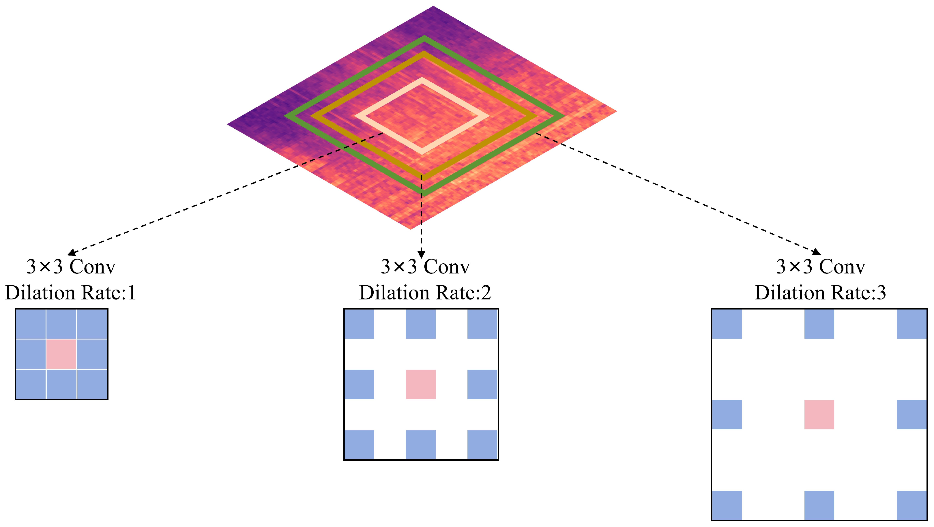
• A Dilated Neighborhood Attention module is introduced in the bottleneck layer of the generator to manage channel interactions and spatial relationships in the intermediate feature maps. This module also accounts for neighborhoods with varying participation rates, enhancing cross-dimensional information interaction between channels and spatial dimensions.
• The reconstruction loss function is redesigned based on the Structure Similarity Index Measure to address inconsistencies in the structure of generated feature maps. This enhancement strengthens the network’s ability to evaluate spectral differences.

2. Related Work

2.1. Reconstruction-Based Anomalous Sound Detection Work

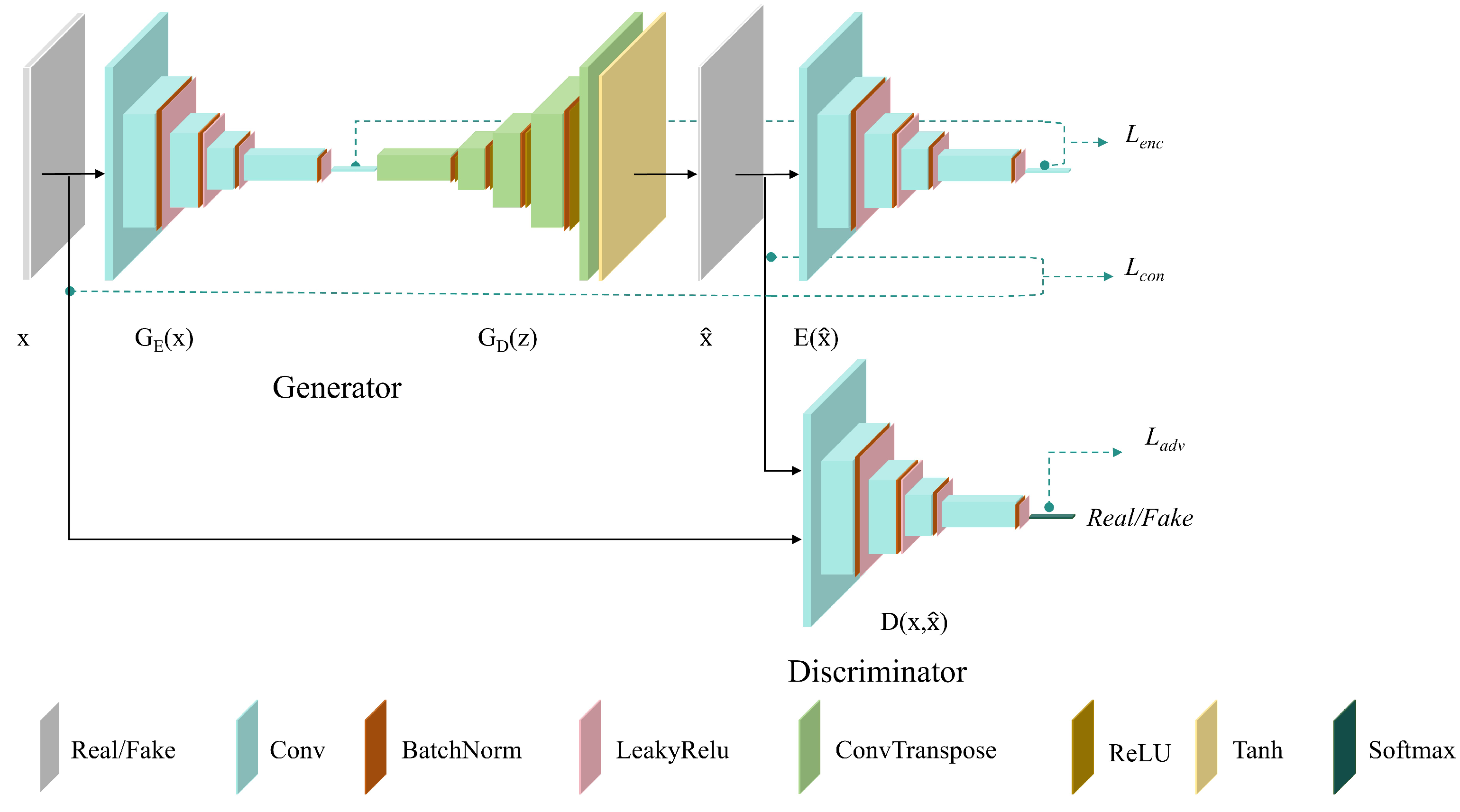
Reconstruction-based models differentiate normal and anomalous data by assessing the reconstruction error produced by a generator network trained on normal data. For example, Tagawa et al. [18] utilized a generative adversarial network to detect anomalies in the sounds of industrial machinery. They utilized the unscented Kalman filter for data preprocessing and introduced a mean squared error loss function with an L2 regularization term. This approach improved detection performance for specific equipment in noisy environments. However, due to the simplicity of the network’s feature engineering design and its neglect of local neighborhood relationships, its detection performance remains suboptimal in complex environments. Liu et al. [19] proposed a generative adversarial network with a multi-attention-enhanced discriminator to emphasize anomalous feature regions in the spectra of mechanical operations. The interaction of channel attention, mel frequency attention, and time attention not only enhances the model’s discriminative ability but also facilitates learning more robust time-frequency features. This approach enables more precise modeling of the time-frequency dynamics of sound, thereby improving the resolution of the discriminator. However, the lack of focus on key features during the reconstruction process may lead to the loss of crucial information when generating feature maps across different dimensions. Chen et al. [20] proposed a multi-scale dual-decoder autoencoder model for domain-shift machine sound anomaly detection. This model integrates fine-grained sound feature information through a multi-scale feature fusion module, enabling effective feature learning across multiple scales and enhancing both model learning capacity and robustness. The multi-scale feature fusion module achieves feature fusion through global feature learning and local feature learning during feature data-dimensional transformation. By integrating information from multiple-scale channels, it mitigates the loss of feature information. However, due to the absence of adversarial training, this approach limits its ability to capture deeper data distribution patterns, thereby weakening the model’s ability to recognize complex patterns. Huang et al. [21] proposed RES-GANomaly for machine sound anomaly detection. This model incorporates an attention mechanism to focus on the continuity of spectral frequency bands, thereby improving reconstruction performance. However, RES-GANomaly only establishes residual connections within the encoder. By introducing residual connections within the generator, information could flow directly from the encoder to the decoder, further mitigating the issue of information loss. To address the strengths and limitations of the aforementioned methods, this paper proposes a reconstruction-based anomaly detection approach that integrates a designed Multi-scale Feature Fusion (MFF) module and a designed Dilated Neighborhood Attention (DNA) module to enhance anomaly detection performance in complex pipeline acoustic environments.

2.2. GANomaly

GANomaly is composed of an encoder $G_E\left(x\right)$, a decoder $G_D\left(x\right)$, a secondary encoder $E\left(\hat{x}\right)$, and a discriminator $D(x,\hat{x})$. The structure of GANomaly is illustrated in Figure 1.

The encoder $G_E\left(x\right)$ transforms the input image into a low-dimensional vector z. Then, the decoder $G_D\left(z\right)$ reconstructs z into an image $\hat{x}$. The second encoder $E\left(\hat{x}\right)$, which has the same structure as the encoder $G_E\left(x\right)$, transforms $\hat{x}$ back into a low-dimensional vector $\hat{z}$. The latent error between the original and reconstructed images is calculated using the low-dimensional vectors z and $\hat{z}$. The discriminator $D(x,\hat{x})$ is used to determine the similarity between generated data and real data, continuously optimizing the gap between them. The goal of using an adversarial strategy is to make the reconstructed data as realistic as possible, rendering it indistinguishable to the discriminator. Minimizing the distance between latent vectors enables the model to approximate the distribution of normal samples. During the testing phase, both reconstruction error and latent error are used as criteria for detecting anomalies. GANomaly utilizes three loss functions as objective constraints: adversarial loss $L_{adv}$, contextual loss $L_{con}$, and encoder loss $L_{enc}$.

2.3. Feature Fusion

Feature fusion serves as a computational strategy to integrate heterogeneous feature representations derived from multi-level input data, thereby synthesizing a unified feature space with enhanced discriminative capacity compared to isolated feature subsets. Therefore, fusing shallow and deep features can effectively balance semantic and detailed information, thereby preventing information loss as the network deepens. Akçay et al. [22] employed skip connections to link the downsampling layers of the encoder in the generator to the corresponding upsampling layers of the decoder. This enhances the detailed information in each dimension, ensuring the generation of high-quality images. Wang et al. [23] introduced an attention gate in GANomaly, enabling the generator to emphasize the most discriminative regions in the spectrum. Zhang et al. [24] applied attention-based feature fusion to the corresponding convolutional layers of the encoder and decoder, preventing key information loss as the network deepens. The aforementioned methods fuse feature maps of the same dimension to enhance information at a single level. However, this may lead to issues such as information redundancy and lack of diversity, limiting the effective enhancement of the network’s expressive capability. In real pipeline scenarios, certain noise signals—such as block noise, grid noise, and valve noise—may only appear at specific times or frequencies. Fusing features at different scales ensures a more comprehensive representation of the noise signals in the pipeline. This paper simultaneously considers spatial and channel information, leveraging the advantages of features from different dimensions for multi-scale feature fusion. This enables a more comprehensive capture of both detailed and semantic information in the input data.

2.4. Attention Mechanism

The attention mechanism dynamically focuses on key features in the input data, helping the model effectively detect anomaly signals while suppressing interference from irrelevant information. Visualization of attention weights allows for an intuitive understanding of the regions or features the model focuses on, thereby enhancing the interpretability of the model. It also establishes correlations between information, enhancing important features while suppressing irrelevant ones. Peng et al. [25] introduced a self-attention mechanism in the encoder output of the generator, fully exploiting the global relationships within normal sample data and focusing on the representative information across multi-scale features. Since the self-attention mechanism prioritizes global information modeling, it may overlook local details, such as subtle changes in short time windows or abrupt high-frequency variations. Zhang et al. [26] designed the scSE attention mechanism to improve the model’s feature representation capability. Notably, these techniques overlook the influence of different spatial and channel neighborhoods. In a spectrum, neighborhoods farther from a specific pixel may carry greater weight than those closer to it. Therefore, this paper proposes a Dilated Neighborhood Attention module that considers neighborhoods with varying participation rates under different receptive fields, preventing abrupt noise features from disrupting the model’s learning of normal data distributions.

3. Methods

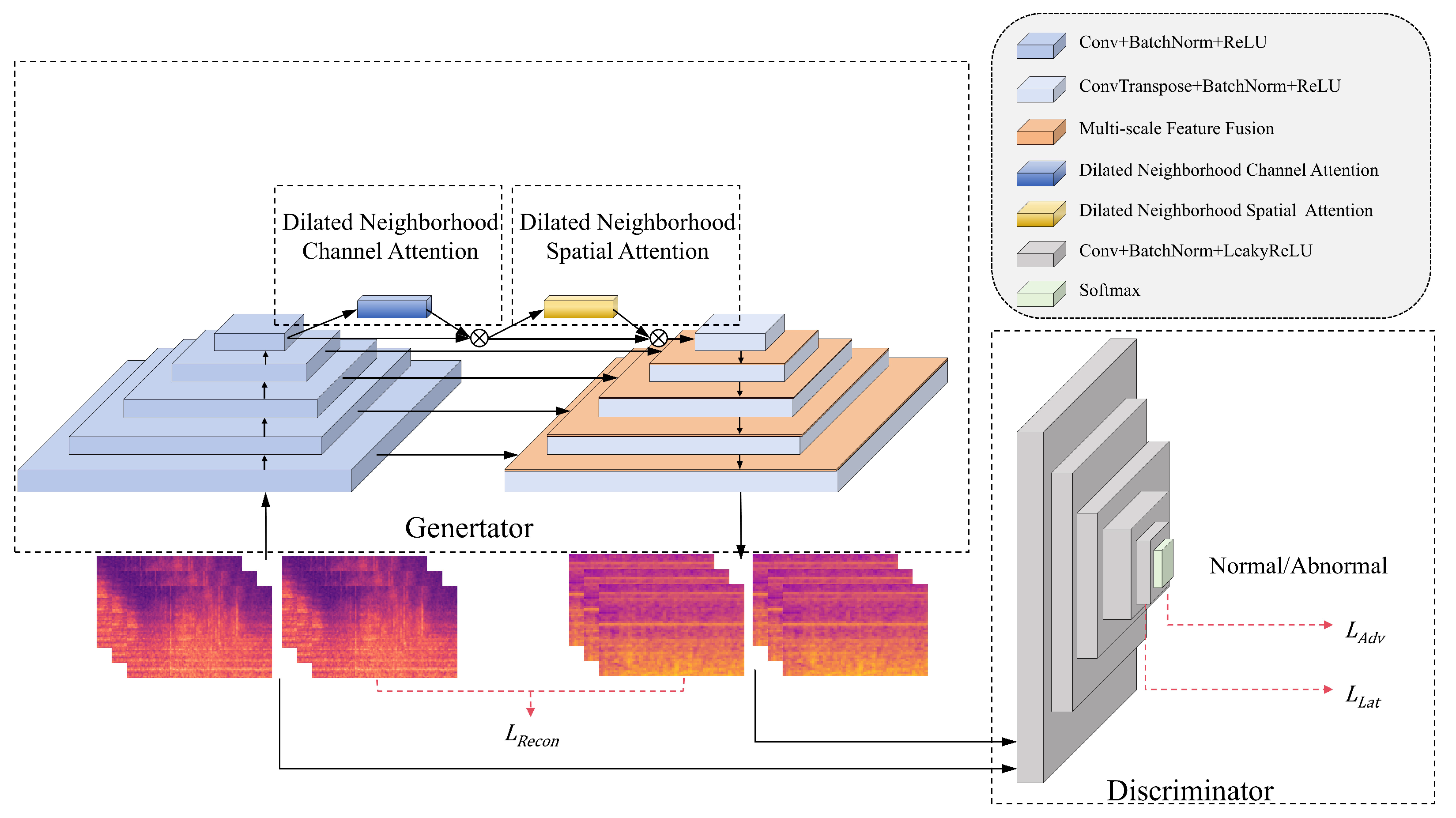
3.1. Overall Architecture of MFDNA-GANomaly

This paper proposes a pipeline anomaly detection method called Multi-scale Feature Fusion GANomaly with Dilated Neighborhood Attention. MFDNA-GANomaly comprises an MFDNA generator and a discriminator, with the network architecture illustrated in Figure 2.

In the MFDNA generator, the primary motivation for removing the second encoder lies in achieving balanced scenario adaptation between model efficiency and detection performance. This architectural simplification mitigates optimization challenges in latent space alignment while enhancing robustness through direct reliance on reconstruction error metrics. Since the second encoder re-encodes the reconstructed output, it can increase the complexity of gradient propagation and exacerbate information loss. Eliminating it simplifies backpropagation and improves the overall stability of model training. The optimized architecture demonstrates closer structural affinity to adversarially trained autoencoders, enabling seamless integration with established detection frameworks. Given that audio data often contain a certain level of noise and variation, and the negative responses of LeakyReLU can help the model better adapt to various distributions of audio data, this paper replaces the traditional ReLU function in the discriminator with the LeakyReLU function to improve the generalization capability of the model.

The generator consists of an encoder and a decoder, as shown in Figure 3. First, the input spectrogram First, the input spectrogram is processed by the generator’s encoder, sequentially producing five feature maps $C_1$, $C_2$, $C_3$, $C_4$, and $C_5$. The designed Dilated Neighborhood Attention module is applied to the encoder output $C_5$, assigning feature weights according to different levels of neighborhood participation, thereby enhancing feature representation. The decoder reconstructs $C_6$, the output of the Dilated Neighborhood Attention module, via transposed convolution to generate $C_7$. To mitigate information loss as the network deepens, a designed Multi-scale Feature Fusion module is introduced after the first four convolutional blocks of the decoder to integrate feature maps of varying dimensions. The Multi-scale Feature Fusion module generates $C_8$, $C_{10}$, $C_{12}$, and $C_{14}$. $C_{14}$ is input into the final convolutional block of the decoder to produce the reconstructed spectrogram. The generator minimizes the reconstruction error $L_{Recon}$ between the original and reconstructed spectrogram, thereby reducing their distance in the latent space and enabling the network to learn the distribution of normal samples. The discriminator consists of a separate encoder and a softmax layer. After receiving both the reconstructed and original spectrograms, the discriminator helps the model learn the data distribution of the input spectrogram by minimizing the latent error $L_{Lat}$. The adversarial training strategy improves the generator’s reconstruction capability and reduces reconstruction error, enabling MFDNA-GANomaly to capture normal data details with higher precision. Consequently, anomalous data exhibit larger reconstruction and latent errors, resulting in a higher anomaly score than normal data.

3.2. Multi-Scale Feature Fusion Module

Information loss is a significant issue during the feature extraction process. To capture more comprehensive feature information, a Multi-scale Feature Fusion (MFF) module is designed. This module integrates input images through global and local variation weight learning, allowing the model to adaptively recalibrate the feature maps. The detailed network architecture is illustrated in Figure 4.

First, the decoded feature map $X\in R^{C_1\times H_1\times W_1}$ is upsampled by a factor of two to obtain a new feature map $X^{\prime }\in R^{C_1\times H\times W}$. The primary purpose of two-fold upsampling is to align the scale, partially restore spatial information lost during downsampling in high-level features, and ensure consistency in the final fused feature dimensions. Then, $X^{\prime }$ is broadcast-added to the encoded feature map $Y\in R^{C\times H\times W}$ to obtain $F\in R^{C\times H\times W}$, where C, H, W represent the number of the channel, height, and width, respectively. Subsequently, the channel and spatial information of F are extracted separately. The formula is as follows:

$$F=X^{\prime }\oplus Y$$

(1)

where ⊕ denotes broadcast addition, and F is the result of the broadcast addition of feature maps.

For channel information, the input feature map F undergoes global average pooling, followed by pointwise convolution to process the global channel information U. The first pointwise convolution reduces the number of channels from C to $C/r$, decreasing parameters and computational load, where r is the scaling factor. Batch normalization and the ReLU activation function are applied to preserve nonlinear characteristics while reducing dimensionality. The second pointwise convolution restores the number of channels from $C/r$ to C. The above operations compress and refine the global channel information, creating a compact representation $G\left(U\right)$ that encapsulates the essential global features. The formulas are as follows:

$$U={\displaystyle \frac{1}{H\times W}}\sum _i^H\sum _j^{W}F(i,j)$$

(2)

$$G\left(U\right)=\mathcal{B}\left(PWCon{\nu }_2\left(\delta \left(\mathcal{B}\left(PWCon{\nu }_1\left(U\right)\right)\right)\right)\right)$$

(3)

where U represents the result of global average pooling, $G\left(U\right)$ represents the global contextual information, $\mathcal{B}$ represents batch normalization, $PWConv$ represents pointwise convolution, and $delta$ represents the ReLU function.

During the extraction of spatial information, two pointwise convolutions are applied sequentially. The first pointwise convolution preserves spatial resolution while processing channel interactions at each spatial location. Following batch normalization and the ReLU function, the second pointwise convolution further refines the features at the same spatial resolution. This branch captures spatial local detail information $L\left(F\right)$. The formula is as follows:

$$L\left(F\right)=\mathcal{B}\left(PWCo{v}_4\left(\delta \left(PWCo{v}_3\left(F\right)\right)\right)\right)$$

(4)

Then, global and local information are fused through broadcast addition, and the values are normalized to the range of 0 to 1 using a sigmoid function to obtain the channel attention weights $F^{\prime }$, which indicate the relative importance of each channel in the input map. The input feature map F is then multiplied element-wise by the channel attention weights to obtain the output map $M\left(F\right)$. Pointwise convolution is used to adjust the channel dimensions of $X^{\prime }$ to obtain $X^{″}$. Finally, the enhanced result is element-wise multiplied with both $X^{″}$ and Y, and the broadcast addition of these results yields the fused feature Z. The formulas are as follows:

$$F^{\prime }=\partial (G\left(U\right)\oplus L\left(F\right))$$

(5)

$$M\left(F\right)=F\otimes F^{\prime }$$

(6)

$$Z=M\left(F\right)\otimes X^{″}\oplus (1-M\left(F\right))\otimes Y$$

(7)

where ∂ represents the sigmoid function, $M\left(F\right)$ represents the fusion weights of multi-scale features, and Z represents the fused feature.

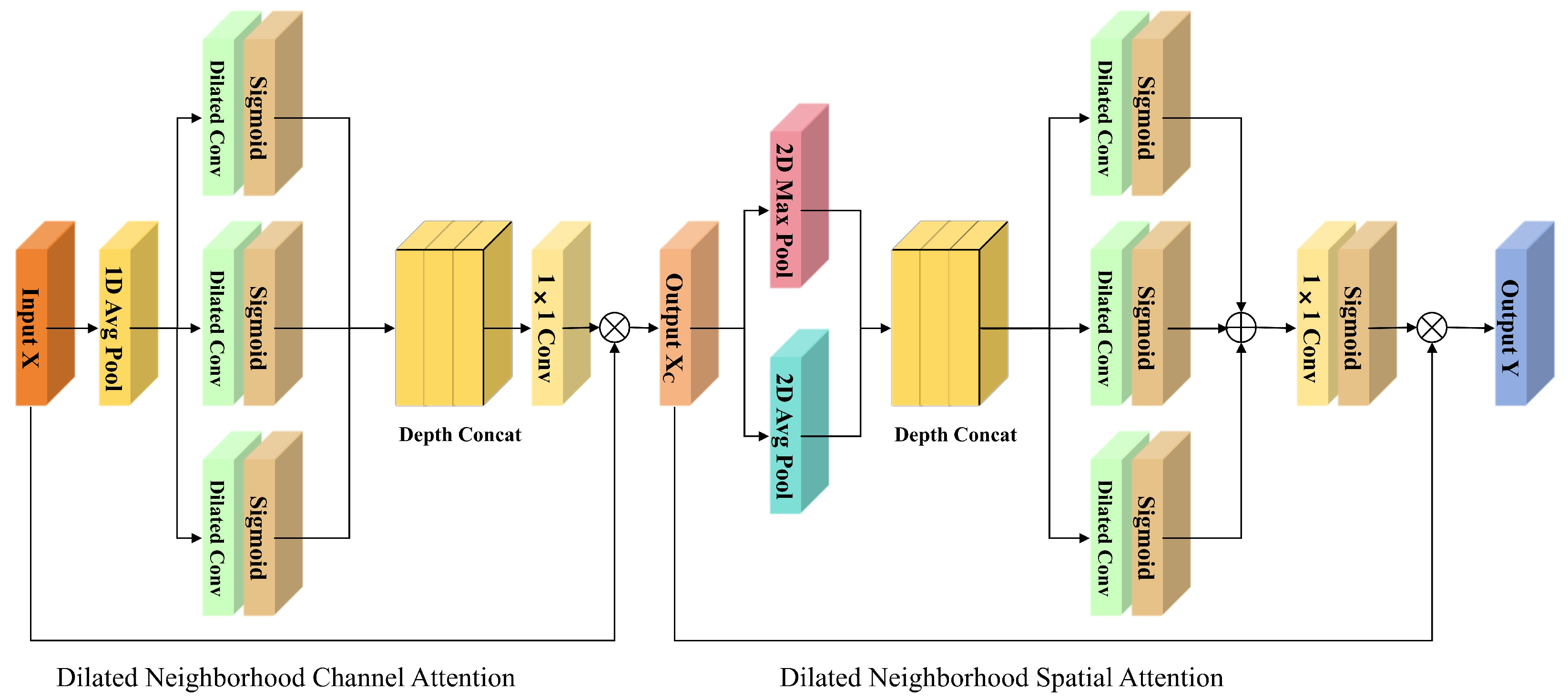
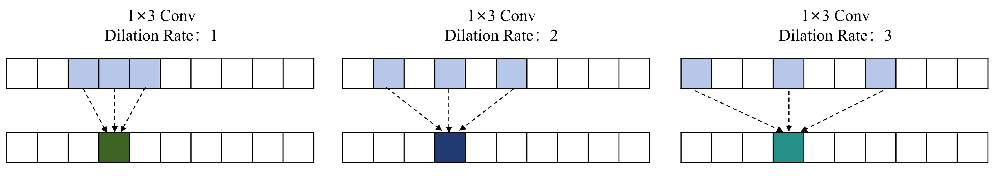
3.3. Dilated Neighborhood Attention Module

To investigate the interrelationships between different neighborhoods in the spectrum, this paper introduces a Dilated Neighborhood Attention (DNA) module. The module, constructed by parallelizing dilated convolutions with various dilation rates and inspired by Atrous Spatial Pyramid Pooling [27], captures broader neighborhood information at multiple scales, enhancing the model’s ability to explore implicit relationships between each pixel and its surrounding neighborhood. The structure of the Dilated Neighborhood Attention is illustrated in Figure 5.

The Dilated Neighborhood Attention module consists of two components: Dilated Neighborhood Channel Attention and Dilated Neighborhood Spatial Attention. In the Dilated Neighborhood Channel Attention, global average pooling is initially applied to compress the height and width of the feature map. This yields channel-level global information denoted as channel-level global information $I_{max}^c\in R^{C\times 1\times 1}$, where C represents the number of the channel. Next, $I_{max}^c$ is input into dilated convolutions with varying dilation rates. Depending on the dilation rate and pixel position, the sigmoid activation function assigns different weight values. The dilation rates are set to varying values of 1, 2, and 3, as illustrated in Figure 6. The channel weight information obtained at each dilation rate is concatenated along the depth dimension. Subsequently, a 1 × 1 convolution is applied to reduce the channel dimensions, resulting in the generation of the Dilated Neighborhood Channel Attention map. Finally, the original input is element-wise multiplied by the Dilated Neighborhood Channel Attention map to produce the adjusted output.

In the Dilated Neighborhood Spatial Attention module, 2D max pooling and average pooling are employed to aggregate the channel information of the feature map, yielding $I_{avg}^s\in R^{1\times H\times W}$ and $I_{max}^S\in R^{1\times H\times W}$, where H and W represent the height and width, respectively. After depth concatenating $I_{avg}^s$ and $I_{max}^s$, dilated convolutions with different dilation rates are applied to extract the spatial neighborhood weight information from the input. The extracted weights are then summed element-wise. In this module, the dilation rates in the Dilated Neighborhood Spatial Attention are set to varying values of 1, 2, and 3, as illustrated in Figure 7. The Dilated Neighborhood Spatial Attention map, obtained through a 1 × 1 convolution and sigmoid activation, assigns varying importance weights to different spatial neighborhoods. The synergy between channel and spatial attention mechanisms enhances the selective and adaptive extraction of information.

3.4. Improved Loss Function

Anomaly detection based on generative adversarial networks generally combines contextual loss, encoder loss, and adversarial loss to minimize the distance between the source and target domains. However, in the detection of audio spectra, the aforementioned loss schemes may neglect the continuity of brightness, contrast, and structural information within the spectrum. To better optimize model parameters during training and reduce the discrepancy between real and reconstructed samples, this paper enhances the contextual loss by incorporating the Structural Similarity Index Measure (SSIM) [28]. This approach reduces reconstruction errors associated with the use of solely Euclidean distance metrics and improves the continuity of frequency band sequences. The SSIM value is determined by both the original image x and the reconstructed image $\hat{x}$. The formula is as follows:

$$SSIM(x,\hat{x})={\displaystyle \frac{(2{\mu }_x{\mu }_{\hat{x}}+a_1)(2{\sigma }_{x\hat{x}}+a_2)}{({\mu }_x^2+{\mu }_{\hat{x}}^2+a_1)({\sigma }_x^2+{\sigma }_{\hat{x}}^2+a_2)}}$$

(8)

where ${\mu }_x$ and ${\mu }_{\hat{x}}$ represent the mean of x and $\hat{x}$, respectively, ${\sigma }_x$ and ${\sigma }_{\hat{x}}$ represent the variance of x and $\hat{x}$, respectively, ${\sigma }_{x\hat{x}}$ represents the covariance of x and $\hat{x}$, and $a_1$ and $a_2$ represent constants. The loss function based on SSIM is as follows:

$$L_{SSIM}(x,\hat{x})=1-SSIM(x,\hat{x})$$

(9)

This paper proposes a combination of contextual loss $L_{con}$ and $L_{SSIM}$ as the image reconstruction loss. The formula is as follows:

$$L_{Recon}=E_{x\sim N_x}[\theta \Vert x-\hat{x} {\Vert }_1+(1-\theta )L_{SSIM}(x,\hat{x})]$$

(10)

where $\theta$ represents the weighting parameters that balance the weights of $L_{con}$ and $L_{SSIM}$; ${∥·∥}_1$ represents the L1-norm. Additionally, the adversarial loss $L_{Adv}$ and the latent loss $L_{Lat}$ are as follows:

$$L_{Adv}=E_{x\sim N_x}[logD\left(x\right)]+E_{x\sim N_x}[log(1-D\left(\hat{x}\right))]$$

(11)

$$L_{Lat}=E_{x\sim N_x}{\Vert f\left(x\right)-f\left(\hat{x}\right) \Vert }_2$$

(12)

where $N_x$ represents the distribution of normal data, D represents the discriminator, $f\left(x\right)$ and $f\left(\hat{x}\right)$ represent the latent features extracted from the original data and reconstructed data, respectively, and ${∥·∥}_2$ represents the L2-norm.

The final overall optimization objective function is formulated as:

$$L={\omega }_{Ad\nu }{L}_{Adv}+{\omega }_{Recon}{L}_{Recon}+{\omega }_{Lat}{L}_{Lat}$$

(13)

where ${\omega }_{Adv}$, ${\omega }_{Recon}$, and ${\omega }_{Lat}$ represent the weighting parameters used to adjust the influence of each loss on the overall optimization objective function. $L_{con}$ is designed to minimize pixel-level error but tends to overlook structural information. $L_{SSIM}$ introduces structural constraints via the SSIM metric, preserving the structural details of frequency bands and compensating for the limitations of $L_{con}$. The combination of $L_{con}$ and $L_{SSIM}$, denoted as $L_{Recon}$, enables the generator to focus on both local pixel accuracy and global structural consistency, thereby enhancing spectral reconstruction capability. The parameter $\theta$ controls the balance between these two factors: as $\theta$ approaches 1, the model emphasizes pixel-level accuracy; as $\theta$ approaches 0, it emphasizes structural similarity. The adversarial loss $L_{Adv}$ drives the generated image distribution to approximate real data but may cause the generator to neglect reconstruction accuracy. $L_{Recon}$ guides the generator in reconstructing the input. However, relying solely on $L_{Recon}$ may result in over-generalization in reconstruction. $L_{Adv}$ and $L_{Recon}$ are dynamically balanced using weight factors ${\omega }_{Adv}$ and ${\omega }_{Recon}$, ensuring the authenticity of generated images while preventing deviation from the input content. The latent loss $L_{Lat}$ regulates the distance between the generated and real images in the discriminator’s feature space, capturing high-level semantic variations. $L_{Lat}$ enhances the robustness of anomaly detection by integrating high-level semantic constraints.

3.5. Anomaly Score

To detect anomalous data in testing and real applications, we use the anomaly score evaluation strategy proposed in [29]. Anomaly score evaluation incorporates both reconstruction error and latent error. The formula is expressed as follows:

$$S\left(x\right)=\gamma \Vert x-\hat{x} {\Vert }_1+(1-\gamma ) {\Vert f\left(x\right)-f\left(\hat{x}\right) \Vert }_2$$

(14)

where x represents the input image, $\hat{x}$ represents the reconstructed image, and $\gamma$ represents the weight parameter.

Finally, $S\left(x\right)$ is scaled to [0, 1] to determine the status of the test data. The farther the scaled value is from the threshold, the higher the probability that the data will be judged as anomalous data. The formula is as follows:

$$S_i={\displaystyle \frac{S\left(x_i\right)-min\left(S\right)}{max\left(S\right)-min\left(S\right)}}$$

(15)

where i represents the ordinal number of the data, $S_i$ represents the anomaly score, which is scaled to [0, 1].

4. Experiments and Result Analysis

4.1. Experimental Introduction

The experiments were conducted on a 64-bit Ubuntu operating system, utilizing the PyTorch 1.9.0deep learning framework and Python 3.7.0 programming language. The detailed information is shown in

Table 1. Hardware equipment and software platform.

Name	Configuration Instruction
Sound Acquisition equipment	Fluke SV600
GPU	NVIDIA A100-SXM
CPU	Intel Xeon Platinum 8375C
Operating System	Ubuntu 18.04.1
Deep Learning Framework	PyTorch 1.9.0 + cu111
Version of Python	3.7.0

.

4.2. Experimental Data

The dataset used in this paper is a custom-built pipeline sound detection dataset. The Fluke SV600 was deployed at critical nodes, including elbows, valves, and joints within the pipeline anomaly simulation setup to systematically collect both normal and anomalous acoustic data under varying diameters and pressure conditions. Each sample is a ten-second, single-channel audio recording containing both pipeline operational sounds and environmental noise. To reflect the rarity of anomalous samples in real-world pipeline scenarios, the dataset maintains a normal-to-anomalous sample ratio of 27:1. In the test set, this ratio is adjusted to 7:3 to facilitate model evaluation. If the proportion of anomalous data is extremely low, the model may achieve a high overall accuracy simply by classifying all instances as “normal”. However, this fails to provide a meaningful assessment of the model’s detection performance. Incorporating an adequate number of anomalous samples enables a comprehensive evaluation of the model’s performance and enhances the realism of the detection scenario simulation. The dataset is partitioned into training, validation, and test sets to ensure a rigorous evaluation of the model’s generalization capability. The training set consists of 2700 normal audio recordings. The recordings are labeled as normal. The training set enables the model to learn the normal operational characteristics of pipeline sounds. The validation set contains 300 normal audio recordings. The recordings are labeled as normal. This set is designed to mitigate overfitting and facilitate the effective learning of normal sound patterns. The test set includes 280 normal and 120 anomalous audio recordings without labels. The test set is exclusively used for final performance evaluation, assessing the model’s ability to distinguish between normal data and anomalous data in real-world scenarios. This partitioning strategy ensures that the training and validation phases focus exclusively on normal sound patterns, preventing any influence from anomalous data.

Additionally, the development dataset from DCASE2023 Task 2 [30] was used to evaluate MFDNA-GANomaly. The dataset comprises seven types of machines. The seven machine types are ToyCar, ToyTrain, Fan, Gearbox, Bearing, Slider, and Valve. For each machine type, a portion of the dataset with representative training and testing data is provided. In the source domain, 990 normal sound clips are used for training. In the target domain, only 10 normal sound clips are utilized. A total of 100 clips of both normal and anomalous sounds are used for testing. The source and target domains for each sample are provided. Mixed data training accounts for the operating conditions of equipment across various environmental and operational states. The source domain primarily contains the majority of the training data and some testing data. The target domain represents a distinct environment where a portion of the training and testing data is recorded. The source and target domains differ in operating speed, load, environmental noise types, and signal-to-noise ratio. This training aims to ensure the adaptability of the model to diverse data distributions and enhance generalization capability.

4.3. Experimental Setup

Through preprocessing, the audio data is transformed into spectrogram data, which serves as the input for model training. First, the 10 s audio signal is sampled at a fixed rate of 16 kHz to maintain a consistent data format. A 2048-point Fast Fourier Transform is applied to transform the time-domain signal into the frequency domain. Then, a hop size of 1024 points and a window size of 2048 points are used for framing, enabling spectral information extraction across different time windows. After framing, 128 mel filters are applied to project the spectrogram to the mel scale. Then, the mel spectrogram is segmented using a sliding window, where each segment has a size of 128 × 128. An overlapping windowing strategy is employed to enable partial data sharing between adjacent segments, enhancing feature continuity.

The model is trained for 100 epochs with a batch size of 128 using the Adam optimizer. The learning rate is set to 0.0002. The Adam optimizer is configured with momentum parameters ${\beta }_1$ = 0.5 and ${\beta }_2$ = 0.999. The generator loss function is weighted using ${\omega }_{Adv}$ = 1, ${\omega }_{Recon}$ = 50, ${\omega }_{Lat}$ = 1, and $\theta$ = 0.65.

4.4. Evaluation Metrics

This paper uses the area under the curve (AUC), partial area under the curve (pAUC), accuracy, and F1-score as evaluation metrics to assess the performance of the model. AUC is unaffected by preset classification thresholds, facilitating a comprehensive evaluation of the performance. Additionally, it demonstrates robust performance for imbalanced datasets. pAUC measures the area under the ROC curve for specific portions, offering a more detailed understanding of the performance of the model in particular regions, such as those with high recall or precision. During the model performance evaluation stage, p = 0.1 is selected. In industrial anomaly detection, maintaining a low false positive rate is essential. Setting p = 0.1 [20] restricts the evaluation to the scenarios where the false positive rate (FPR) ranges from 0 to 0.1, enabling a more precise assessment of the model’s detection capability under stringen false positive constraints. Pipeline system maintenance and monitoring incur significant costs. A high false positive rate may trigger unnecessary maintenance activities, increasing operational costs. Therefore, achieving high detection accuracy while minimizing the false positive rate is critical. Further reducing the p range may impose overly stringent constraints, leading to an overly conservative model evaluation. An excessively conservative evaluation may fail to detect true anomalies, increasing the false negative rate and thereby degrading overall detection performance. Moreover, it may fail to adequately capture the model’s robustness and adaptability in real-world scenarios, hindering further model optimization. Therefore, setting p = 0.1 provides a more realistic reflection of the model’s practical applicability in industrial environments.

$Accuracy$ is the ratio of correctly predicted samples to the total number of samples. The F 1-score is the harmonic mean of $precision$ and $recall$. $Accuracy$, $precision$, $recall$, and F 1-score are obtained using an optimal threshold of 0.3. The formulas are as follows:

$$Accuracy={\displaystyle \frac{TP+TN}{TP+TN+FP+FN}}$$

(16)

$$Precision={\displaystyle \frac{TP}{TP+FP}}$$

(17)

$$Recall={\displaystyle \frac{TP}{TP+FN}}$$

(18)

$$F1=2\times {\displaystyle \frac{Precision\times Recall}{Precision+Recall}}$$

(19)

where $TP$ represents the number of samples predicted by the model as positive that are actually positive, $TN$ represents the number of samples predicted as negative that are actually negative, $FP$ represents the number of samples predicted as positive but are actually negative, and $FN$ represents the number of samples predicted as negative but are actually positive.

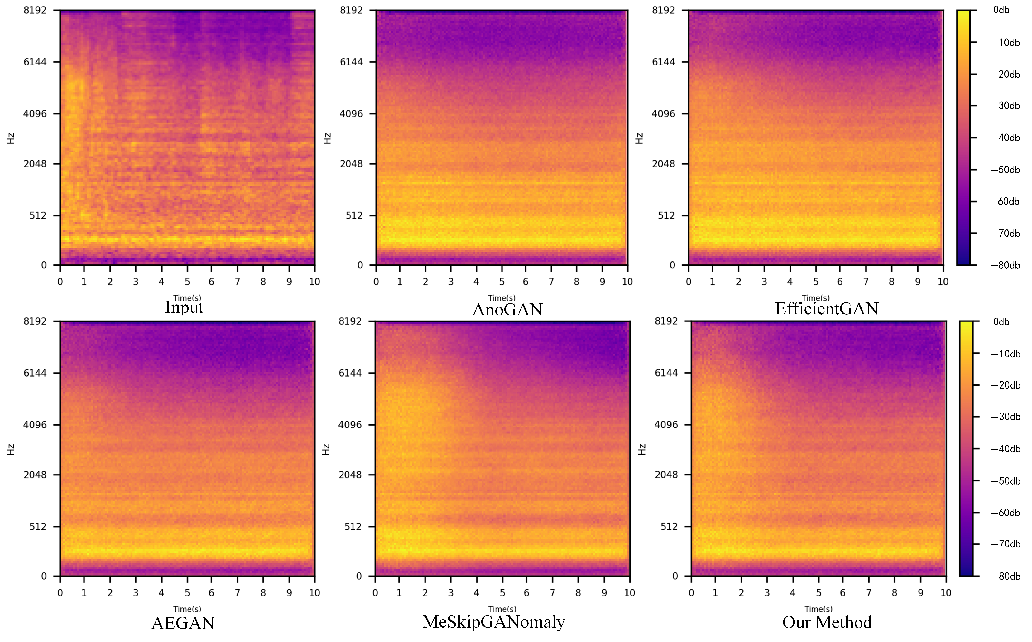
4.5. Comparative Experiment

Four models, AnoGAN [29], EfficientGAN [31], AEGAN [32], and MeSkipGANomaly [33], are selected to be compared to the proposed method on the test set of the gas distribution network. Results are shown in

Table 2. Comparison of experimental results for test set.

Method	AUC/%	pAUC/%	Accuracy/%	F1-Score
AnoGAN	71.65	50.58	74.87	0.809
EfficientGAN	73.84	57.95	81.40	0.861
AEGAN	83.19	60.47	85.92	0.896
MeSkipGANomaly	86.79	65.89	89.44	0.921
Our Method	92.06	64.92	93.96	0.955

.

As can be seen from the above table, MFDNA-GANomaly achieved the best performance with AUC (92.06%), Accuracy (93.96%), and F1-score (0.955). The pAUC of our method is 64.92%, which is lower than that of MeSkipGANomaly. The number of skip connections is adjusted, and MeSkipGANomaly also introduces a memory enhancement module to refine learned sample mapping, which explains its superior performance in regions with low false positive rates. The superior performance of MeskipGANomaly on the pAUC metric helps reduce false alarms in pipeline anomaly detection. Compared to the other three methods, our approach achieved a higher pAUC. This indicates that while outperforming other models in anomaly detection across various classification thresholds, MFDNA-GANomaly also maintains high sensitivity at lower false positive rates. MFDNA-GANomaly achieves a well-balanced performance across multiple evaluation metrics, leading to superior overall effectiveness.

Additionally, the reconstructed spectra for each model are analyzed. As shown in Figure 8, when a normal spectrum is input, the loss of detail in the reconstructed spectra of the four comparison models is primarily reflected in variations in color intensity. The proposed MFDNA-GANomaly not only enhances the sequential correlation within the frequency bands of the spectrum but also mitigates energy information loss in each band. As shown in Figure 9, when an anomalous spectrum is input, the reconstructed spectra of the four comparison models are affected by the presence of anomalous information. The reconstructed anomalous spectrum from MFDNA-GANomaly contains minimal anomalous information, indicating that the model effectively captures the characteristics of normal data. The proposed method achieves high-fidelity background reconstruction in the mid-to-high frequency domain, producing an energy distribution that closely matches that of the input image. AnoGAN is unable to provide an effective reconstruction image, and EfficientGAN exhibits pronounced attenuation in the low-frequency region compared to the input image. MeSkipGANomaly and the proposed method show marginally improved low-frequency reconstruction relative to EfficientGAN; however, residual energy loss persists. The observed information loss in the low-frequency domain may result from persistent noise, causing the model to emphasize high-frequency structures. Future research may focus on diversifying training data and refining the loss function to improve low-frequency reconstruction quality.

To verify the generalization capability of our proposed MFDNA-GANomaly, we also conducted a comparative analysis on the DCASE Challenge 2023 Task2. We selected three types of models for comparison across seven audio datasets. The selected methods are described as follows. Zhao et al. [34] proposed an integrated system that combines GAN and AE models, utilizing spectra and log-mel energy for training. Fujimura et al. [35] tackled anomaly detection using ResNet-18 as a feature extractor. Wilkinghoff [36] introduced a hybrid model combining static and dynamic frequency information, enhancing detection performance through auxiliary classification tasks. The comparison of our method with other approaches is presented in

Table 3. AUC and pAUC results for the development dataset from DCASE2023 Task 2.

Method	Metric	ToyCar	ToyTrain	Fan	Gearbox	Bearing	Slider	Valve
AE-GAN-AD [34]	${\mathrm{AUC}}_s$/%	74.22	70.66	81.32	73.80	75.48	89.10	43.18
	${\mathrm{AUC}}_t$/%	54.44	59.04	62.56	69.74	67.70	67.38	43.04
	${\mathrm{pAUC}}_{s-t}$/%	49.68	51.26	59.42	59.84	58.00	64.11	49.05
Fujimural et al. [35]	${\mathrm{AUC}}_s$/%	62.36	68.88	78.04	83.72	74.44	96.14	97.62
	${\mathrm{AUC}}_t$/%	62.48	55.24	70.96	79.44	57.40	91.88	98.68
	${\mathrm{pAUC}}_{s-t}$/%	51.53	48.58	70.32	64.26	56.26	80.53	78.95
Wilkinghoff et al. [36]	${\mathrm{AUC}}_s$/%	60.66	58.12	80.22	82.66	75.48	94.02	87.98
	${\mathrm{AUC}}_t$/%	50.04	61.64	64.76	80.92	71.64	93.72	88.96
	${\mathrm{pAUC}}_{s-t}$%	48.02	48.37	52.32	65.21	51.42	72.68	87.47
Our Method	${\mathrm{AUC}}_s$/%	75.78	68.42	75.34	87.56	74.93	92.34	94.53
	${\mathrm{AUC}}_t$/%	63.23	62.45	58.32	81.92	72.46	80.68	92.49
	${\mathrm{pAUC}}_{s-t}$/%	55.42	56.74	62.65	69.97	59.92	70.90	76.34

.

The experiments demonstrate that our model exhibits excellent performance in terms of AUCt and pAUC of the ToyTrain and Bearing subsets. On the Gearbox subset, the scores for the three evaluation metrics all surpassed the comparison model, with scores of 87.56%, 81.92%, and 69.97%, respectively. Our model demonstrates strong performance at low false positive rates on the ToyTrain, Bearing, and Gearbox subsets, indicating robust generalization capabilities. However, there is still room for improvement in Fan and Slider, due to notable differences between the sound composition of these devices and the training data used in this study. Given that data in real-world scenarios are influenced by external factors, domain shifts are likely to occur. Therefore, the performance metrics of the target domain are more indicative of practical applicability compared to those of the source domain.

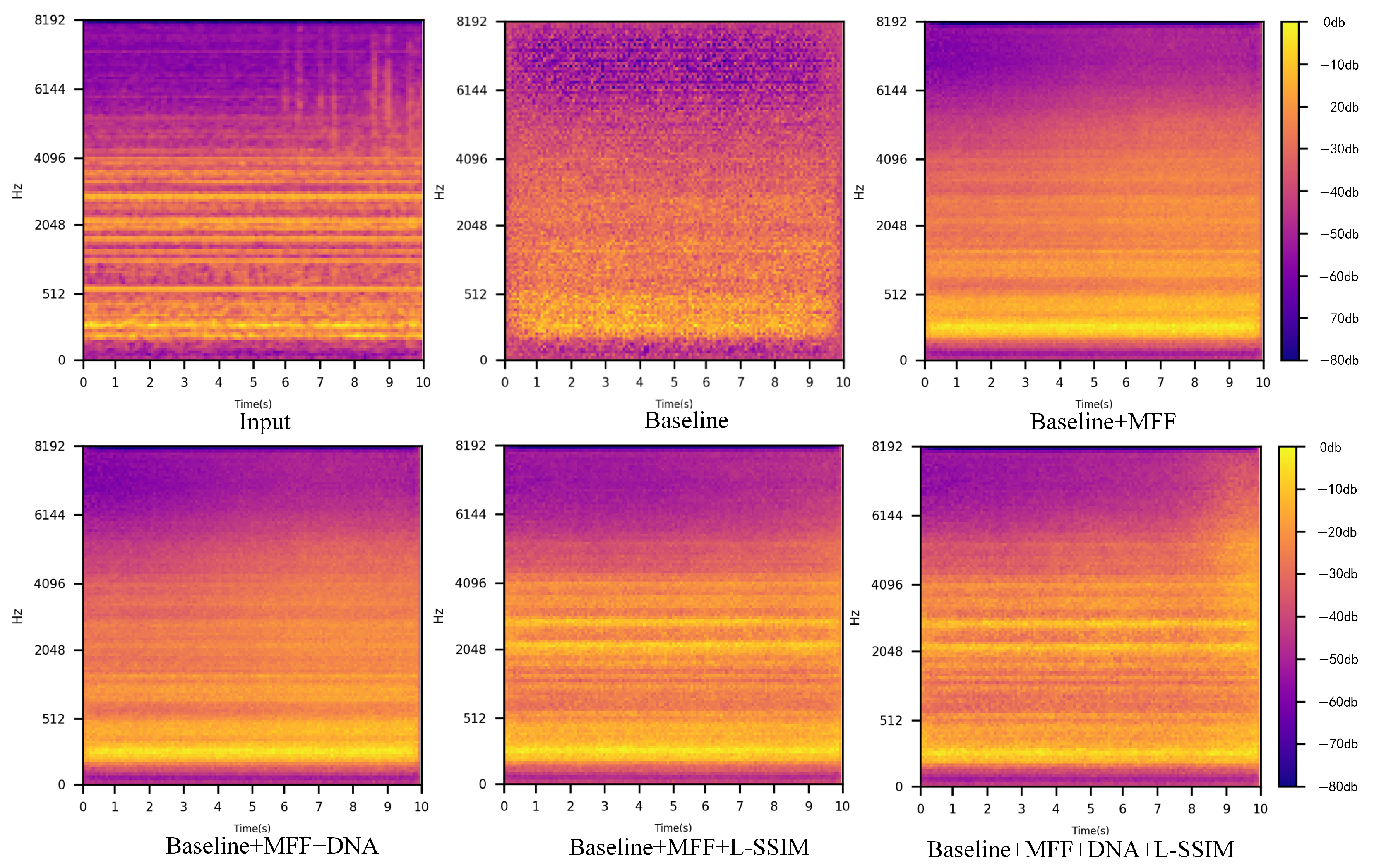
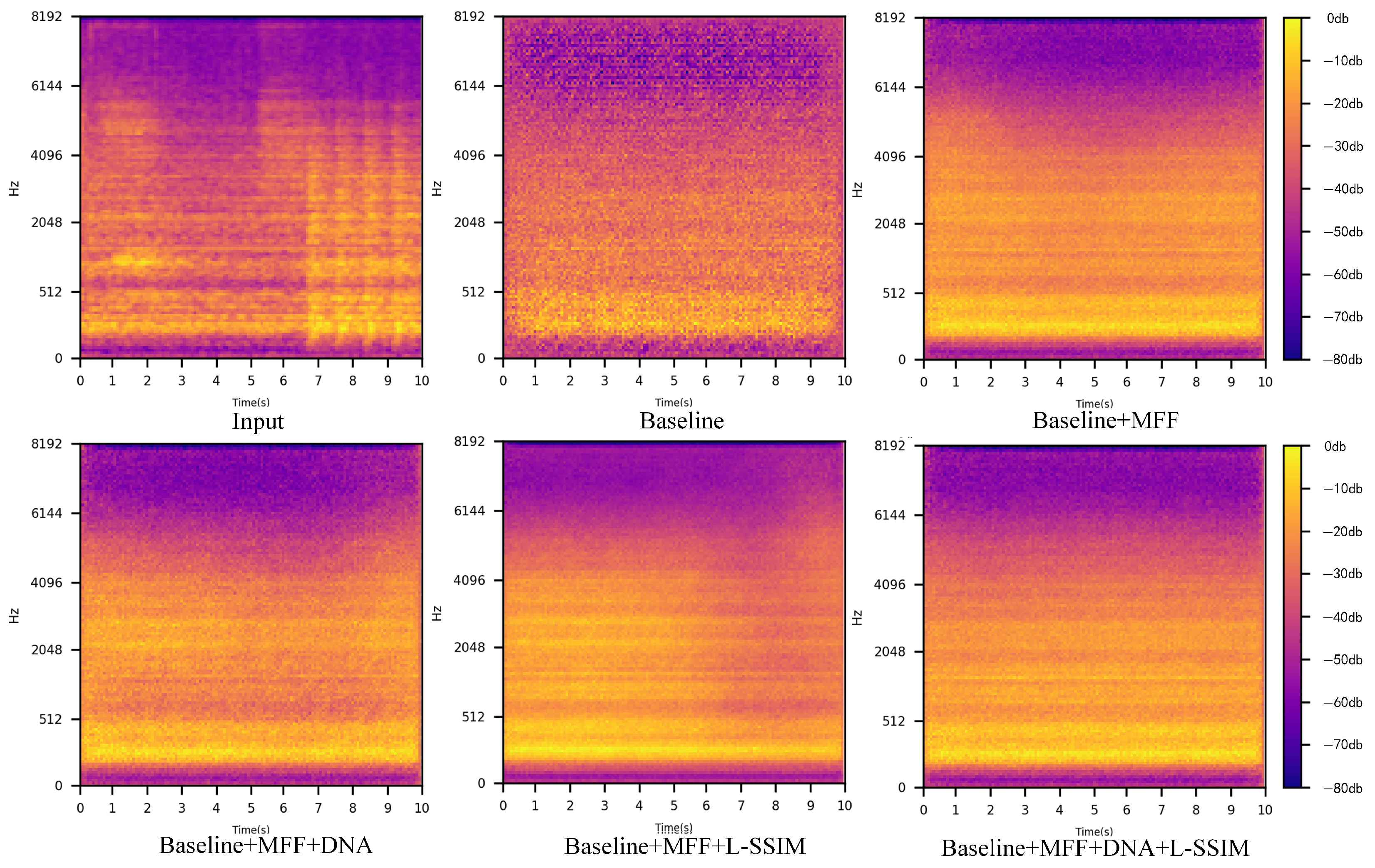
4.6. Ablation Experiment

To examine the correlation and effects of the Multi-scale Feature Fusion module, the Dilated Neighborhood Attention (DNA) module, and the SSIM-based improved loss function within MFDNA-GANomaly, corresponding ablation experiments were conducted, as shown in

Table 4. Comparison of ablation results for test set.

Baseline	MFF	DNA	L-SSIM	AUC/%	pAUC/%	Accuracy/%	F1-Score
✓				74.67	61.46	73.86	0.810
✓	✓			81.51	61.84	84.92	0.889
✓	✓	✓		83.19	63.47	88.94	0.919
✓	✓		✓	86.82	62.73	91.54	0.941
✓	✓	✓	✓	92.06	64.92	93.96	0.955

.

Incorporating the Multi-scale Feature Fusion (MFF) on the Baseline enhances AUC, Accuracy, and F1-score by 6.84%, 11.06%, and 0.07, respectively. Further improvement in overall performance is achieved by adding the Dilated Neighborhood Attention (DNA) module and the SSIM-based improved loss function L-SSIM to Baseline + MFF. This suggests that Dilated Neighborhood Attention assists the model in capturing neighborhood weight relationships at different receptive fields, enhancing the intensity integrity of spectral pixels. Additionally, the improved loss function L-SSIM accounts for the structural correlation and other information in complex pipeline audio data, improving the accuracy of actual pipeline anomaly detection. The pAUC of Baseline + MFF + L-SSIM is lower than that of Baseline + MFF + DNA, suggesting that Dilated Neighborhood Attention has a more pronounced effect on the model at low false-positive rates. After incorporating all key components, MFDNA-GANomaly achieves the best performance across all metrics.

A visual analysis of the reconstructed images from all methods in the ablation experiments is presented. As shown in Figure 10, the MFDNA generator provides superior reconstruction results for normal data.

Figure 11 demonstrates that the model cannot effectively reconstruct anomalous data. Consequently, the reconstructed spectra contain only minimal anomalous information, increasing the reconstruction error for anomalous spectra. MFDNA-GANomaly effectively improves the reconstruction of the normal spectra while suppressing that of the anomalous spectra. Due to the lack of key modules, the baseline model can only learn part of the distribution of normal data. The reconstructed images lack detailed information and show no sequential correlation in the energy across different frequency bands. The integration of Multi-scale Feature Fusion improves the overall reconstruction quality of Baseline + MFF, but some detailed information is still missing. Adding Dilated Neighborhood Attention and L-SSIM further preserves more low-frequency and high-frequency energy distribution information in the reconstructed images.

Figure 12 presents the histogram of anomaly scores from the test phase. The histogram reveals a clear distinction between normal and anomalous data, with normal scores clustering at lower values and anomalous scores at higher values, indicating effective separation. The bell-shaped distribution of normal scores suggests the model captures typical data behavior, which is advantageous for detecting anomalies in structured datasets. The minimal overlap between normal and anomalous scores underscores the potential for high precision in anomaly detection. However, the histogram also reveals that there is a noticeable overlap between normal and anomalous scores from 0.3 to 0.35, making it challenging to distinguish between these samples solely by their anomaly scores. If the threshold is set too low, normal samples may be misclassified as anomalous, leading to a higher false positive rate. Conversely, if the threshold is set too high, anomalous samples may be misclassified as normal, resulting in a higher false negative rate. This overlapping region suggests the presence of borderline cases in anomaly detection, which may stem from measurement errors, environmental noise, or inherent variations in data distribution. To address these overlapping regions, an optimal threshold can be determined through ROC curve analysis or partial AUC (pAUC), ensuring a balance between false positive and false negative rates. An uncertainty interval can be defined between 0.3 and 0.35, permitting manual review of a small subset of data within this range. While the model effectively distinguishes between normal and anomalous data, additional refinements could reduce score overlap and mitigate biases in anomaly score distributions.

Figure 13 presents the t-SNE visualization of features extracted from the last convolutional layer of the discriminator. In both Figure 12 and Figure 13 anomaly scores and features of normal data are distinctly separated from those of anomalous data, demonstrating that the proposed method exhibits strong separability in both output anomaly scores and features.

5. Discussion

Although MFDNA-GANomaly has shown good performance, it still has several limitations. First, if anomalous data exhibit diverse patterns and some anomalous samples share similar features with normal samples, the model may struggle to accurately capture these distinctions, leading to distribution overlap. Future work will explore the integration of multimodal data to enhance anomaly detection capability. Second, the lack of an effective visualization strategy constrains the interpretability of the model. This limitation hinders the model’s ability to identify fault types. To address this limitation, an advanced visualization technique should be incorporated. Grad-CAM [37] is an emerging technique that leverages gradient-weighted feature maps for anomaly detection without necessitating modifications to the network architecture. It propagates gradients to the final convolutional layer, producing a coarse localization map. The attention-based Grad-CAM method [38,39] incorporates attention mechanisms to highlight key regions essential for classification, demonstrating superior performance across diverse domains. Its visualization capabilities enhance model interpretability. Additionally, compared to autoencoder-based approaches, GAN-based methods require higher computational resources and longer processing times. To fulfill real-time industrial requirements, future work will focus on optimizing lightweight models to reduce computational complexity and developing efficient detectors for time-frequency localization. By leveraging these advanced techniques, future research aims to refine pipeline anomaly detection methods, thereby improving both the intelligence and generalization of detection systems.

6. Conclusions

This paper proposes a Multi-scale Feature Fusion GANomaly with Dilated Neighborhood Attention (MFDNA-GANomaly) for pipeline anomaly detection to address the challenges of data imbalance, varying environmental noise, and complex operating conditions. MFDNA-GANomaly integrates multi-dimensional information through the Multi-scale Feature Fusion module, primarily tackling the issue of original information loss in the reconstruction process of the generator. In the bottleneck layer of the generator, a designed Dilated Neighborhood Attention module is employed to capture channel interactions and spatial relationships across different neighborhoods, enriching the feature representation of the reconstructed data. The improved loss function, based on structural similarity, enhances the continuity and structural consistency of the generated normal spectra. Through the analysis of experimental results, the effectiveness of the proposed model in reducing information loss and improving generalization ability is verified. The model achieved 92.06% AUC, 93.96% accuracy, and 0.955 F1-score on the pipeline sound dataset. In summary, the model meets the requirements for detection accuracy and precision in pipeline anomaly detection tasks under complex working conditions.

References

1. Li, F.; Zheng, H.; Li, X.; Yang, F. Day-ahead city natural gas load forecasting based on decomposition-fusion technique and diversified ensemble learning model. Appl. Energy 2021, 303, 117623. [Google Scholar]
2. Chen, J.; Wang, S.; Liu, Z.; Guo, Y. Network-based optimization modeling of manhole setting for pipeline transportation. Transp. Res. E Logist. Transp. Rev. 2018, 113, 38–55. [Google Scholar]
3. Bian, X.; Li, Y.; Feng, H.; Wang, J.; Qi, L.; Jin, S. A location method using sensor arrays for continuous gas leakage in integrally stiffened plates based on the acoustic characteristics of the stiffener. Sensors 2015, 15, 24644–24661. [Google Scholar] [CrossRef] [PubMed]
4. Liu, C.; Li, Y.; Xu, M. An integrated detection and location model for leakages in liquid pipelines. J. Pet. Sci. Eng. 2019, 175, 852–867. [Google Scholar]
5. Li, X.; Zhao, T.; Sun, Q.; Chen, Q. Frequency response function method for dynamic gas flow modeling and its application in pipeline system leakage diagnosis. Appl. Energy 2022, 324, 119720. [Google Scholar]
6. Zhou, Y.; Zhang, Y.; Yang, D.; Lu, J.; Dong, H.; Li, G. Pipeline signal feature extraction with improved VMD and multi-feature fusion. Syst. Sci. Control Eng. 2020, 8, 318–327. [Google Scholar]
7. Liu, C.W.; Li, Y.X.; Yan, Y.K.; Fu, J.T.; Zhang, Y.Q. Technical analysis and research suggestions for long-distance oil pipeline leakage monitoring. J. Loss Prev. Process Ind. 2015, 35, 236–246. [Google Scholar]
8. Wang, W.; Gao, Y. Pipeline leak detection method based on acoustic-pressure information fusion. Measurement 2023, 212, 112691. [Google Scholar]
9. Wu, Y.; Ma, X.; Guo, G.; Huang, Y.; Liu, M.; Liu, S.; Zhang, J.; Fan, J. Hybrid method for enhancing acoustic leak detection in water distribution systems: Integration of handcrafted features and deep learning approaches. Process Saf. Environ. Prot. 2023, 177, 1366–1376. [Google Scholar]
10. Wang, C.; Han, F.; Zhang, Y.; Lu, J. An SAE-based resampling SVM ensemble learning paradigm for pipeline leakage detection. Neurocomputing 2020, 403, 237–246. [Google Scholar]
11. Yang, D.; Hou, N.; Lu, J.; Ji, D. Novel leakage detection by ensemble 1DCNN-VAPSO-SVM in oil and gas pipeline systems. Appl. Soft Comput. 2022, 115, 108212. [Google Scholar]
12. Yao, L.; Zhang, Y.; He, T.; Luo, H. Natural gas pipeline leak detection based on acoustic signal analysis and feature reconstruction. Appl. Energy 2023, 352, 121975. [Google Scholar]
13. Deng, X.; Xiao, L.; Liu, X.; Zhang, X. One-dimensional residual GANomaly network-based deep feature extraction model for complex industrial system fault detection. IEEE Trans. Instrum. Meas. 2023, 72, 3520013. [Google Scholar]
14. Hu, Z.; Wang, L.; Qi, L.; Li, Y.; Yang, W. A novel wireless network intrusion detection method based on adaptive synthetic sampling and an improved convolutional neural network. IEEE Access 2020, 8, 195741–195751. [Google Scholar]
15. Ma, X.; Keung, J.; He, P.; Xiao, Y.; Yu, X.; Li, Y. A semisupervised approach for industrial anomaly detection via self-adaptive clustering. IEEE Trans. Ind. Inform. 2023, 20, 1687–1697. [Google Scholar]
16. Han, Y.; Chang, H. Xa-ganomaly: An explainable adaptive semi-supervised learning method for intrusion detection using ganomaly. Comput. Mater. Contin. 2023, 76, 221–237. [Google Scholar]
17. Akcay, S.; Atapour-Abarghouei, A.; Breckon, T.P. GANomaly: Semi-supervised Anomaly Detection via Adversarial Training. In Proceedings of the 14th Asian Conference on Computer Vision (ACCV), Perth, Australia, 2–6 December 2018; pp. 622–637. [Google Scholar]
18. Tagawa, Y.; Maskeliūnas, R.; Damaševičius, R. Acoustic anomaly detection of mechanical failures in noisy real-life factory environments. Electronics 2021, 10, 2329. [Google Scholar] [CrossRef]
19. Liu, S.; Li, J.; Ke, W.; Yin, H. Multi-Attention Enhanced Discriminator for GAN-Based Anomalous Sound Detection. In Proceedings of the IEEE International Conference on Acoustics, Speech and Signal Processing (ICASSP), Seoul, Republic of Korea, 14–19 April 2024; pp. 6715–6719. [Google Scholar]
20. Chen, S.; Sun, Y.; Wang, J.; Wan, M.; Liu, M.; Li, X. A multi-scale dual-decoder autoencoder model for domain-shift machine sound anomaly detection. Digit. Signal Process. 2024, 156, 104813. [Google Scholar]
21. Huang, X.; Guo, F.; Chen, L. A RES-GANomaly method for machine sound anomaly detection. IEEE Access 2024, 12, 80099–80114. [Google Scholar]
22. Akçay, S.; Atapour-Abarghouei, A.; Breckon, T.P. Skip-ganomaly: Skip connected and adversarially trained encoder-decoder anomaly detection. In Proceedings of the International Joint Conference on Neural Networks (IJCNN), Budapest, Hungary, 14–19 July 2019; pp. 1–8. [Google Scholar]
23. Wang, Y.; Jiang, Z.; Wang, Y.; Yang, C.; Zou, L. Intelligent detection of foreign objects over coal flow based on improved GANomaly. J. Intell. Fuzzy Syst. 2024, 46, 5841–5851. [Google Scholar]
24. Zhang, L.; Dai, Y.; Fan, F.; He, C. Anomaly Detection of GAN Industrial Image Based on Attention Feature Fusion. Sensors 2022, 23, 355. [Google Scholar] [CrossRef] [PubMed]
25. Peng, J.; Shao, H.; Xiao, Y.; Cai, B.; Liu, B. Industrial surface defect detection and localization using multi-scale information focusing and enhancement GANomaly. Expert Syst. Appl. 2024, 238, 122361. [Google Scholar] [CrossRef]
26. Zhang, H.; Qiao, G.; Lu, S.; Yao, L.; Chen, X. Attention-based Feature Fusion Generative Adversarial Network for yarn-dyed fabric defect detection. Text. Res. J. 2023, 93, 1178–1195. [Google Scholar]
27. Chen, L.C.; Zhu, Y.; Papandreou, G.; Schroff, F.; Adam, H. Encoder-decoder with atrous separable convolution for semantic image segmentation. In Proceedings of the European Conference on Computer Vision (ECCV), Munich, Germany, 14–19 September 2018; pp. 801–818. [Google Scholar]
28. Bergmann, P.; Löwe, S.; Fauser, M.; Sattlegger, D.; Steger, C. Improving Unsupervised Defect Segmentation by Applying Structural Similarity to Autoencoders. Available online: https://arxiv.org/abs/1807.02011 (accessed on 5 July 2024).
29. Schlegl, T.; Seeböck, P.; Waldstein, S.M.; Schmidt-Erfurth, U.; Langs, G. Unsupervised Anomaly Detection with Generative Adversarial Networks to Guide Marker Discovery. Available online: https://arxiv.org/abs/1703.05921 (accessed on 20 March 2024).
30. Purohit, H.; Tanabe, R.; Ichige, K.; Endo, T.; Nikaido, Y.; Suefusa, K.; Kawaguchi, Y. MIMII dataset: Sound dataset for malfunctioning industrial machine investigation and inspection. In Proceedings of the Detection and Classification of Acoustic Scenes and Events 2019 Workshop (DCASE2019), New York, NY, USA, 25–30 June 2019; pp. 1–19. [Google Scholar]
31. Zenati, H.; Foo, C.; Lecouat, B.; Manek, G.; Chandrasekhar, V. Efficient Gan-Based Anomaly Detection. Available online: https://arxiv.org/abs/1802.06222 (accessed on 17 February 2024).
32. Jiang, A.; Zhang, W.; Deng, Y.; Fan, P.; Liu, J. Unsupervised anomaly detection and localization of machine audio: A gan-based approach. In Proceedings of the IEEE International Conference on Acoustics, Speech and Signal Processing (ICASSP), Rhodes Island, Greece, 4–10 June 2023; pp. 1–5. [Google Scholar]
33. Jiang, W.; Yang, K.; Qiu, C.; Xie, L. Memory enhancement method based on Skip-GANomaly for anomaly detection. Multimed. Tools Appl. 2024, 83, 19501–19516. [Google Scholar]
34. Zhao, Z.; Tan, Y.; Qian, K.; Xu, K.; Hu, B. Ensemble Systems with GAN and Auto-Encoder Models for Anomalous Sound Detection. Available online: https://dcase.community/documents/challenge2023/technical_reports/DCASE2023_QianXuHu_95_t2.pdf (accessed on 10 June 2024).
35. Fujimura, T.; Kuroyanagi, I.; Hayashi, T.; Toda, T. Anomalous Sound Detection by End-to-End Training of Outlier Exposure and Normalizing Flow with Domain Generalization Techniques. Available online: https://dcase.community/documents/challenge2023/technical_reports/DCASE2023_Fujimura_75_t2.pdf (accessed on 10 June 2024).
36. Wilkinghoff, K. Fraunhofer FKIE Submission for Task 2: First-Shot Unsupervised Anomalous Sound Detection for Machine Condition Monitoring. Available online: https://dcase.community/documents/challenge2023/technical_reports/DCASE2023_Wilkinghoff_4_t2.pdf?utm_source=chatgpt.com (accessed on 10 June 2024).
37. Selvaraju, R.R.; Cogswell, M.; Das, A.; Vedantam, R.; Parikh, D.; Batra, D. Grad-cam: Visual explanations from deep networks via gradient-based localization. In Proceedings of the IEEE International Conference on Computer Vision (ICCV), Venice, Italy, 22–29 October 2017; pp. 618–626. [Google Scholar]
38. Chen, H.Y.; Lee, C.H. Vibration signals analysis by explainable artificial intelligence (XAI) approach: Application on bearing faults diagnosis. IEEE Access 2020, 8, 134246–134256. [Google Scholar]
39. Raghavan, K.; Kamakoti, V. Attention guided grad-CAM: An improved explainable artificial intelligence model for infrared breast cancer detection. Multimed. Tools Appl. 2024, 83, 57551–57578. [Google Scholar] [CrossRef]
Figure 1. Architecture of GANomaly.
Information 16 00279 g001
Figure 2. Architecture of the Multi-scale Feature Fusion GANomaly with Dilated Neighborhood Attention.
Information 16 00279 g002
Figure 3. Generator of MFDNA-GANomaly.
Information 16 00279 g003
Figure 4. Multi-scale Feature Fusion module.
Information 16 00279 g004
Figure 5. Dilated Neighborhood Attention module.
Information 16 00279 g005
Figure 6. Convolution kernels with different dilation rates in Dilated Neighborhood Channel Attention.
Information 16 00279 g006
Figure 7. Convolution kernels with different dilation rates in Dilated Neighborhood Spatial Attention.
Information 16 00279 g007
Figure 8. The input normal spectrum and the reconstructed spectra from different models.
Information 16 00279 g008
Figure 9. The input anomalous spectrum and the reconstructed spectra from different models.
Information 16 00279 g009
Figure 10. The input normal spectrum and the reconstructed spectra from different variants.
Information 16 00279 g010
Figure 11. The input anomalous spectrum and the reconstructed spectra from different variants.
Information 16 00279 g011
Figure 12. Histogram of scores for 200 test samples.
Information 16 00279 g012
Figure 13. t-SNE visualization of the features of 200 test data extracted by the last convolutional layer of the discriminator.
Information 16 00279 g013