ADFilter—A Web Tool for New Physics Searches with Autoencoder-Based Anomaly Detection Using Deep Unsupervised Neural Networks

Abstract

A web-based tool called ADFilter (short for Anomaly Detection Filter) was developed to process collision events using autoencoders based on a deep unsupervised neural network. The autoencoders are trained on a small fraction of either collision data or Standard Model (SM) Monte Carlo simulations. The tool calculates loss distributions for input events, helping to determine the degree to which the events can be considered anomalous with respect to the SM events used for training. Therefore, it can be used for new physics searches in collider experiments. Real-life examples are provided to demonstrate how the tool can be used to reinterpret existing results from the Large Hadron Collider (LHC), with the goal of significantly improving exclusion limits. This tool is expected to mitigate the “reproducibility crisis” associated with various machine learning techniques, as it can incorporate machine learning approaches from third-party publications, making them accessible to the general public.

1. Introduction

Traditionally, searches for new physics involve applying selection cuts to target phase spaces where sensitivity to Beyond Standard Model (BSM) phenomena is highest [1]. These cuts are typically designed by exploring the kinematics of BSM events or using some general principles of how new physics might modify events produced by Standard Model (SM) processes.

Alternatively, selections can be performed by creating neural networks that “remember” the primary kinematic characteristics of collected data events, which are predominantly governed by SM processes. The events that closely match these characteristics are then removed, leaving only those that are anomalous in some way from the main body of events. This selection method requires no prior knowledge of BSM models, making it more agnostic to potential new physics. This creates a unique opportunity to search for new physics in phase-space regions that have never been probed by traditional searches. The main goal of such methods is to explore the rich final states produced at the Large Hadron Collider (LHC), which have never been probed [2] using traditional labor-intensive approaches based on BSM models. An overview of anomaly detection methods is provided in [3]. Anomaly-detection methods based on deep learning are widely used across various fields of study [4,5].

ATLAS recently published the first article [6] utilizing anomaly detection to identify LHC events with the five types of reconstructed objects (jets, b-jets, electrons, muons, and photons) most likely to be present in BSM scenarios. In this approach, Autoencoders (AEs) are trained on a small fraction of the collected data to determine the global characteristics of their event kinematics. The trained AE is then applied to the rest of the data that need to be tested. By analyzing the loss distributions, or the errors with which the AE reproduces the data, one can select only events with large AE losses. This process identifies outlier events that deviate significantly from the bulk of events, which are dominated by SM processes. The neural network approach is expected to capture full correlations between various inputs, making it superior to methods that rely purely on statistical measures to determine how unique an event is. Once an “anomalous” region of phase space with large loss values for events is determined, it must be further investigated using various techniques. The ATLAS study [6] used searches in dijet invariant masses in the anomaly region to detect BSM signals. Additional demonstrations of this method using Monte Carlo (MC) simulations are provided in [7,8].

From an experimental standpoint, the advantages of such approaches are clear: These model-agnostic selections lead to an improved sensitivity to BSM phenomena. However, if BSM signals are not found, experimental limits should be calculated for events in the outlier region. Such limits should include acceptance corrections, which are difficult to estimate outside the LHC experiments.

Thus, to facilitate comparisons of data in the outlier region with proposed BSM models, a simple public tool is needed that can propagate event records from any arbitrary BSM model and report the acceptances in the anomaly regions as defined by experiments. This approach to anomaly detection requires the wide public availability of trained autoencoders. These AEs, trained on a portion of data (or SM MC simulations), will represent the kinematics of data (or SM processes) and can thus be used to calculate acceptance for any BSM model.

This paper introduces a new online tool called “ADFilter” [9], an abbreviation that originates from “Anomaly Detection Filter”. The purpose of this tool is to process event records from collision events (such as those generated by Monte Carlo simulations) through AEs used in physics research. It calculates the AE loss distribution for collision events, and then it applies a selection cut, accepting only events within the anomaly region. This functionality enables the evaluation of acceptance corrections, which are calculated as the ratio of events that pass the AE cut to the total number of input events. Therefore, ADFilter is crucial for comparing BSM scenarios with data in anomaly regions. The goal of this tool is to mitigate the “reproducibility crisis” associated with various machine learning techniques, as it can incorporate machine learning approaches from third-party publications, making them accessible to the general public. Until now, no such tools have existed in particle physics.

The structure of this paper is as follows: Section 2 describes ADFilter from the user’s perspective. Section 3 provides a detailed technical implementation. A real-life example is discussed in Section 4, followed by the Conclusions. The Appendix outlines the structure of data records used as inputs and presents an example of how this tool can be used to reinterpret published exclusion limits for new particle searches.

2. Description of ADFilter

The ADFilter (Anomaly Detection Filter) webpage [9] features the user interface shown in Figure 1. The public version includes the AEs described in [6,8]. The LHC paper [6] employs a subset of the Run 2 ATLAS data, while the second paper relies on SM MC simulations for AE training. The autoencoder uses selection criteria based on single-lepton triggers, accepting events with at least one lepton with transverse momentum $p_T^l>60$ GeV. This cut effectively reduces the multijet background, which dominates the LHC data.

To start event processing, one needs to select the AE using a drop-down menu and then upload a file with input events. The formats for the input files are discussed in Section 3. The maximum size of the input file is 150 MB, which is typically sufficient for about 100,000 events in the file format to be discussed later.

After uploading, the ADFilter interface will submit several jobs in order to create the following:

• A ROOT file with the inputs for AE and a few test histograms. This ROOT file’s name ends with the string “rmm.root”. It contains basic kinematic distributions, the histogram “cross” with the observed cross-section (in pb), the Rapidity–Mass Matrix (RMM) [10] for the first 50 events (for demonstration purposes), and the ROOT tree “inputNN”, which stores non-zero values for the RMM and their indices.
• A ROOT file with the final result. The name of this ROOT file contains the substring “ADFilter”. It includes a histogram called “Loss”, representing the numerical value of the reconstruction loss after processing through the AE. This histogram shows the success of the encoder–decoder process in reconstructing the compressed input. The “EventFlow” histogram shows the number of events entering the AE and the number of output events that exceed the “LossCut” value, which is typically defined in the relevant publications. The output ROOT file also includes a set of histograms showing invariant masses before and after the AE, as well as the cross-section in the selected anomalous region.
• A text file that contains information about all processing steps. This file has the extension “.log”. It can be used to monitor and verify each step of data processing, from the file with the input variables to the final file with the loss distribution. It also prints the selection cuts used for event processing.

All ROOT histograms can be viewed using the online browser and can also be downloaded for offline analysis.

It should be noted that if the input file contains only partons, this tool also applies parton showering and hadronization using the Pythia8 [11] generator. This creates an intermediate binary file with the extension “promc”, which includes all final-state particles. All technical details on how to use ADFilter are given in the menu called “Documentation”.

The web interface of ADFilter is implemented in the PHP language with an external call to a binary program that converts the input data to ROOT files containing the tree with the input for the AE. The autoencoder calls were implemented in Python3. The jsROOT package [12] was used to display the ROOT output files online.

3. Technical Details on Input Files and Event Processing

The ADFilter web tool accepts a variety of input files containing collision events. These input files must be generated with the same center-of-mass collision energy as the events used for AE training. Figure 2 shows the diagram demonstrating the workflow of ADFilter, starting from the input files to the final results. In the following, we will describe these steps in more detail.

The preferred event record should include the four-momentum of jets (including light-flavor jets and jets associated with b-quarks), electrons, muons, photons, and missing transverse energy. The jet definition should match the one used in the AE. An example of the generic input data structure is provided in Appendix A. The data format is a simple TTree called “Ntuple”. An additional histogram (“meta”) stores metadata with the center-of-mass energy (in GeV) used, whereas another histogram (“cross”) contains the generator-level cross-section (in pb) and the luminosity (in pb⁻¹) for the current run.

There are other types of input files that do not include reconstructed jets and leptons. These inputs can either be events with the four-momentum of final-state particles or files containing parton-level information. In the latter case, as previously mentioned, ADFilter propagates the events through the parton shower and hadronization. Then it applies jet reconstruction, isolation criteria for leptons, and the necessary transverse-momentum cuts as specified for the selected AE.

In the following, we briefly describe the input files that can be used by ADFilter.

3.1. Delphes Input Files

The tool accepts ROOT ntuples generated by the Delphes fast simulation [13]. However, because the input files can be quite large, Delphes files must be reduced in size (“slimmed”). To facilitate this, a simple tool is provided, as detailed on the “Documentation” page. This tool reduces the Delphes file to the smallest event structure that ADFilter can accept, as illustrated in Appendix A.

It is important to minimize selection cuts on Delphes objects to avoid introducing biases when using the AE. Generally, applying transverse momentum cuts of 30 GeV for all jets, leptons, and photons is the safest approach.

3.2. Truth-Level Event Record

To upload truth-level information with final-state particles, one can use ProMC files [14]. These files are based on Google’s Protocol Buffers, which are a language-neutral, platform-neutral, and extensible mechanism for serializing structured data. They use “varints” as a way to store and compress integers using a variable number of bytes. Smaller numbers use fewer bytes. This means that low-energy particles (jets, clusters, cells, tracks, etc.) can be represented with fewer bytes since the values needed to represent such particles are smaller compared to those of high-energy particles or other objects.

ProMC files can be created directly from Monte Carlo generators or downloaded from the HepSim repository [15], where about 350 event samples are stored in the ProMC format.

3.3. LHE Parton-Level Files

One can also upload LHE files (Les Houches Event Files) [16] directly from the Madgraph generator [17,18]. The files should be compressed and have the extension *.lhe.gz. ADFilter applies the parton showering and hadronization. These steps are performed by the Pythia8 [11] generator. The output events with final-state particles are stored in the ProMC file format, which is available for download.

3.4. Object Reconstruction Step

Collision events stored in binary ProMC files are processed with the goal of reconstructing jets, b-jets, isolated leptons, and photons. The jet definition and selection cuts are configured to match the objects used during AE training.

Jets, isolated electrons, and muons were reconstructed from stable particles. The jets were constructed with the anti-$k_T$ algorithm [19], as implemented in the FastJet package [20] with a distance parameter of $R=0.4$, which is commonly used in the ATLAS experiment. By default, the minimum transverse energy of all jets was 30 GeV in the pseudorapidity range of $\left|\eta \right|<2.5$, but these values may change depending on the selection used by the AEs.

Leptons are required to be isolated using a cone of size $0.2$ in the azimuthal angle and pseudorapidity defined around the true direction of the lepton. All energies of particles inside this cone are summed. A lepton is considered isolated if it carries more than $90\%$ of the cone energy. The SM background processes require simulations of misidentification rates for muons and electrons (“fake rates”). We used a misidentification rate of 0.1% for muons and 1% for electrons. This is implemented by assigning a probability of ${10}^{-3}$ (${10}^{-2}$) for a jet to be identified as a muon (electron) using a random number generator. The distributions were obtained for events having at least one isolated lepton with transverse momentum $p_T^l>30$ GeV and two jets with $p_T^j>30$ GeV.

3.5. Pre-Processing Step

The current version of ADFilter includes two autoencoder architectures, as previously mentioned, which require a pre-processing step to create input data for AEs. This step is described in this section. However, it is important to note that ADFilter is not limited to these two architectures; as a web tool, it can implement any autoencoder described in public research papers.

After all objects (jets, leptons, and photons) are available, a C++ program is used to transform the kinematic features of each event to the RMM, which is proposed as an input for machine learning [10]. The RMM is a square matrix that includes reconstructed final states of jets, b-jets, muons, electrons, photons, and $E_T^{miss}$, where $E_T^{miss}$ is a single object, followed by 10 (b-)jets and 5 electrons, muons, and photons each, in descending order of transverse energy for each particle type. This matrix contains characteristics of individual and pairwise combinations of considered objects, filled with zeros to the matrix rows and columns, where the corresponding objects are undetected. In particular, the transverse energy of the leading objects or the transverse energy imbalances of the rest objects concerning the leading one in each object type is placed along the diagonal, where the transverse energy imbalance is defined as the ratio between their difference in the transverse energy and their sum. The non-diagonal upper-right values of the matrix are the invariant mass of the corresponding two objects represented by the row and the column; in the case where $E_T^{miss}$ is above 50 GeV, the transverse mass is used instead. All values in the diagonal and above are scaled by $1/\sqrt{s}$, where $\sqrt{s}$ is the collision energy. The non-diagonal lower-left values are $h_{ij}=C·(\cosh ((y_i-y_j)/2)-1)$, where $y_i-y_j$ represents the rapidity difference between the two objects i and j; when j is $E^{miss}$, $h_i=C·(\cosh \left(y_i\right)-1)$ is used instead. The constant C was set to $0.15$ [10].

By construction, all elements of the RMM are defined to be between 0 and 1, and most variables are Lorentz-invariant under boosts along the longitudinal axis. To reduce biases in the shapes of the jet+Y invariant mass spectra, the nine invariant mass variables are excluded from the RMM. The resulting input dimension is ${36}^2-9=1287$. The RMM matrix is then flattened to a one-dimensional input vector before being fed into the AE.

3.6. Autoencoder Step

To demonstrate ADFilter’s capabilities, we will now describe the two autoencoders that are currently implemented. After a ROOT file with the tree containing non-zero values of the RMMs was created, this tree was used as an input for the trained AE. The autoencoder is typically trained on a small fraction of real collision events or the SM MC simulations, thus the weights of neurons represent the snapshot of known physics events. Training is not covered in this paper since it is specific to each analysis domain. During the file upload, the user should select the desired AE whose description is usually given in the specific publication.

The AE is implemented using TensorFlow [21]. It comprises two sections, an encoder and a decoder. The encoder compresses the input to a latent dimensional space, whereas the decoder takes the data in the latent layer and decompresses it back to its original size. The network architecture for the encoder contains two hidden layers, with 800 and 400 neurons, respectively, and a latent layer of 200 neurons. The decoder reverses the structure of the encoder, using 400 and 800 neurons for the two hidden layers, and 1287 neurons for the output layer. The AE architecture was optimized using tests with artificially created “anomalous” events by misidentifying objects in the Monte Carlo simulated events. The architecture reflects object multiplicities, particle identifications, and their kinematic characteristics well. The Leaky ReLU [22] activation function is applied to the output in all hidden and output layers.

The final result of the AE step is to produce a ROOT file with invariant masses before and after applying a selection cut on the loss. The value of the selection cut is predetermined by previous publications.

The entire analysis chain, from the input file to the ROOT file with RMM and then the Python code with TensorFlow [21], was implemented using the BASH language. The website framework uses PHP with an external call to the master BASH script that executes the entire processing chain.

The public version of ADFilter uses the AE described in [6] trained on the Run2 LHC data with single-lepton pre-selections. In addition, the ADFilter menu includes an AE trained on the SM events, as explained in [8]. The source code of the ADFilter is publicly available from the GIT repository [23].

The ADFilter can also be used as a command-line tool in the LXPLUS computing environment, as described in the menu “Documentation”.

4. Real-Life Examples

The LHC publications that focus on exclusion limits typically apply loose pre-selections guided by BSM model expectations. For example, one can apply a transverse momentum cut on leptons $p_T^l>60$ GeV in situations where high-momentum leptons are expected for certain BSM scenarios [24]. More sophisticated selections use boosted decision trees or neural networks trained on specific BSM events. While the first approach does not have the best sensitivity to BSM models, the second approach with improved sensitivity is significantly more time-consuming to develop.

As discussed in the Introduction, another approach is to evaluate limits after applying AEs to reject the trivial SM background. In this approach, a single trained AE can be used for a large variety of BSM scenarios as long as event triggering is appropriate. To calculate limits after the AE, experimental data should be available in the anomaly region. Then, to set competitive exclusion limits, the BSM models need to be propagated through the same AE.

This is where the ADfilter should be in hand: If the limits in the anomaly region are available from LHC publications and the HEPdata database [25], this tool helps estimate acceptance corrections for BSM events in order to compare the acceptance-corrected cross-section with limits in anomaly regions. The easiest BSM models for testing are those that create well-defined enhancements in two-body invariant masses. Because the tool reconstructs invariant masses before and after cuts on the AE loss distribution, the acceptance can be easily estimated. In this section, two examples of how to use ADFilter for two concrete BSM models are given. This check normally takes 3–5 min using the ADFilter website.

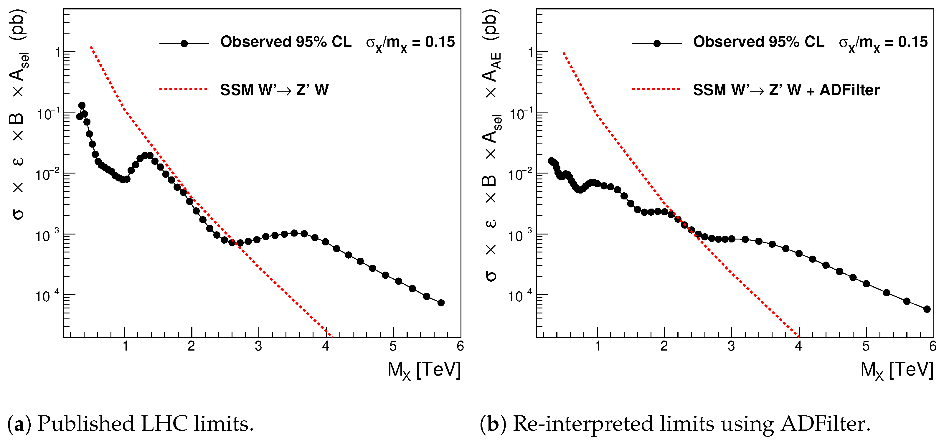
4.1. Re-Interpretation of Sequential-Standard Model Limits

In the first example, we will utilize the publicly available data used to exclude the Sequential-Standard Model (SSM) with the $W^{\prime }\to Z^{\prime }{W}^{\pm }$ process [24]. The published 95% CL upper limits are available as a function of masses $M_X$. For the SSM, X represents masses of $Z^{\prime }$ extracted from the invariant mass of two jets, i.e., $M_{jj}$. Events were pre-selected by placing the transverse momentum cut $p_T^l>60$ GeV on leptons (electrons or muons). These limits are expressed in terms of $\sigma \times B$, where $\sigma$ is a cross-section, and B is a branching ratio. The limits [24] are reproduced as black diamonds in Figure 3a. The red line shows the SSM model predictions. The original exclusion, reported in [24], was at 2 TeV, where black diamonds overlap with the red dashed line. Experimentally, such limits are corrected by the factors $A_{sel}\times \epsilon$ as a function of the mass $M_X$, where $A_{sel}$ is the acceptance introduced by the event and object selection, and $\epsilon$ is an object reconstruction efficiency. Such factors are known and available from publications.

The generic limits as a function of $M_X$ after applying the cut $p_T^l>60$ GeV and the AE are available [6] and tabulated in HEPdata [6]. These limits were calculated for the resonance width of $\sigma /M_X=0.15$, which is similar to the SSM studied in [24]. These limits are obtained after the AE selection, therefore, they are expressed in terms of $\sigma \times B\times \epsilon \times A_{sel}\times A_{AE}$, where $A_{sel}$ is the traditional acceptance introduced by event/object selections, and $A_{AE}$ is the acceptance introduced by the AE.

The factor $A_{sel}\times \epsilon$ is common to both [6,24] publications, as long as selection cuts are the same. Therefore, one can multiply the limits [6] by the correction factors $1/(A_{sel}\times \epsilon )$ obtained from [24]. After this correction, one obtains the limits in terms of $\sigma \times B\times A_{AE}$. These limits are shown in Figure 3b with the blue-filled circles. They are substantially lower than those expressed in terms of $\sigma \times B$, as the trained AE significantly reduces the rate of SM events (i.e., $A_{AE}<1$).

In order to perform exclusions, the BSM model shown in Figure 3a needs to be re-interpreted in terms of $\sigma \times B\times A_{AE}$. To do this, ADFilter can be used to estimate the ADFilter acceptance $A_{AE}$. This can be done by using an MC generator at the truth level to produce $W^{\prime }\to Z^{\prime }{W}^{\pm }$ events for different mass points and uploading the generated LHE files to the ADFilter website. Our calculations estimate that the ADFilter acceptance is 55% for SSM (on average). Then, the BSM prediction shown in [24] should be multiplied by these acceptances as a function of $Z^{\prime }$ mass.

The final result of the re-interpretation of the limit is shown in Figure 3b. After anomaly detection, the mass exclusion moves from 2 TeV to 2.5 TeV, where the blue-filled circles overlap with the brown dotted line representing SSM corrected by the ADFilter acceptance. This demonstrates that the application of the AE can increase the exclusion region by roughly 500 GeV.

It should be pointed out that our discussion assumes that the limits for Gaussian signals with a width of 15% are directly applicable to exclude the SSM. For high-precision studies, the availability of experimental limits for different realistic signal shapes in the anomaly region is highly desirable.

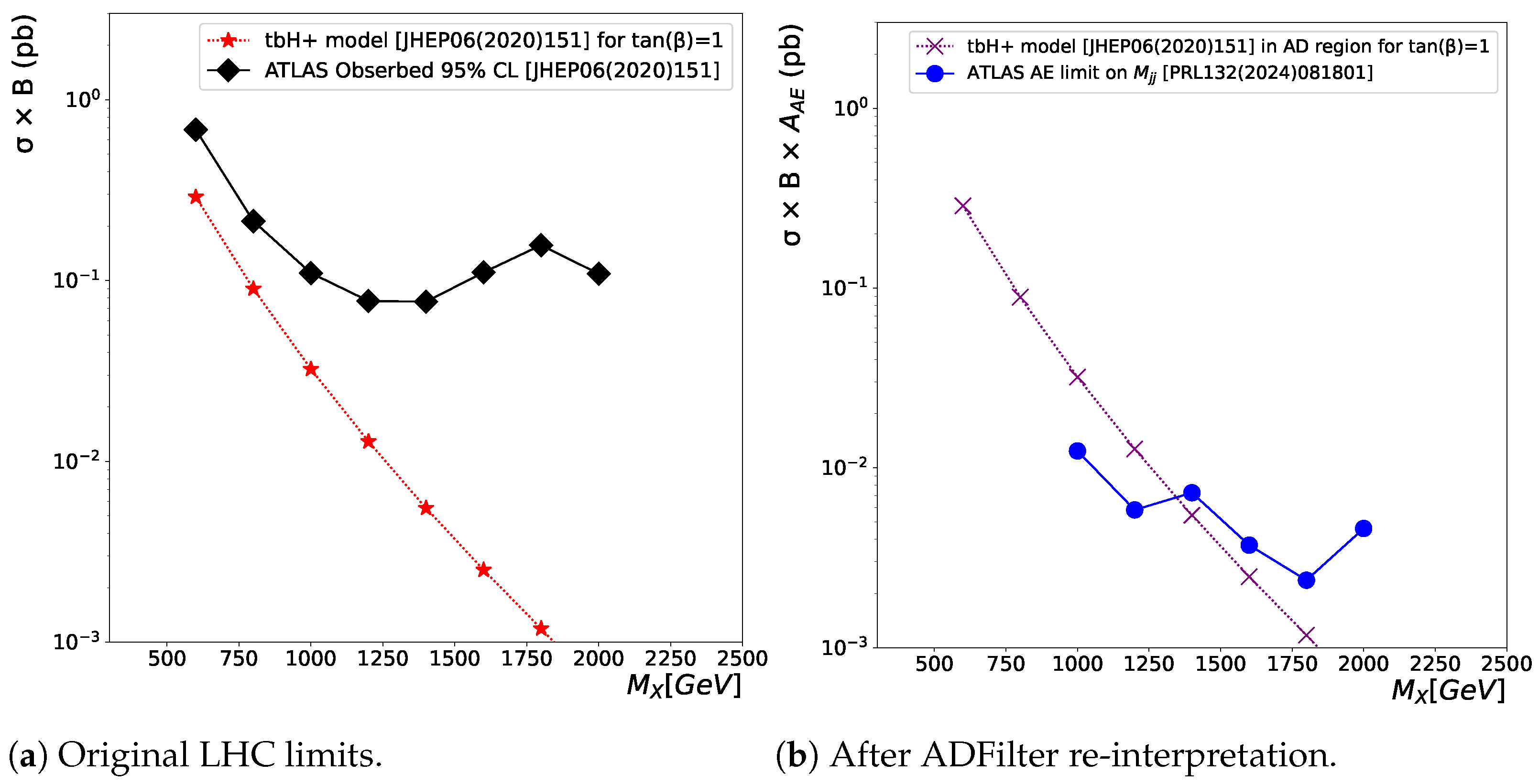
4.2. Re-Interpretation of Charged Higgs $tb{H}^{+}$ Limits

Our second example is related to the charged Higgs $tb{H}^{+}$ process [24]. This process was modeled with MadGraph5_aMC@NLO [18] at Next-to-Leading Order (NLO) in QCD [26] based on a two-Higgs-Doublet Model (2HDM) using a four-flavor scheme implementation. In this model, $tan\left(\beta \right)$ is the ratio of the two scalar doublets in the 2HDM. Figure 4a reproduces the ATLAS observed limit (shown with black diamond symbols) for the pre-selection $p_T^l>60$ GeV as a function of the dijet mass and the $tb{H}^{+}$ process cross-sections (red dotted line) for $tan\left(\beta \right)=1$. The limits are shown as a function of $M_X$, where X represents a $H^{+}$ mass derived from the mass of two jets, $M_{jj}$. The $tb{H}^{+}$ process cross-section does not overlap with the observed limits, indicating that the data do not have sufficient statistical power to exclude this BSM model with $tan\left(\beta \right)=1$.

The situation changes drastically when applying ADFilter. Figure 4b shows the limit with $p_T^l>60$ GeV plus the AE selection [6] for signals with a width of $\sigma /M_X=0.15$. These limits were multiplied by the factor $1/(A_{sel}\times \epsilon )$, as reported in [24]. To justify this correction, we assume that the width of $M_{jj}$ for the $tb{H}^{+}$ process is roughly similar to the width $\sigma /M_X=0.15$. Then, the ADFilter was used to estimate the AE correction for the charged Higgs $tb{H}^{+}$ process created with MadGraph5_aMC@NLO. According to the calculated ADFilter acceptance, the observed cross-section for the $tb{H}^{+}$ process does not change significantly after applying anomaly detection, since the reported ADFilter acceptance was above 95%. The large AE acceptance indicates that the $tb{H}^{+}$ events are highly anomalous, compared to the SM events represented by the AE. Figure 4b shows the limit with the cut $p_T^l>60$ GeV plus the AE selection [6] for signals with the width of $\sigma /M_X=0.15$. This creates a crossing point of the observed limits (shown with blue-filled circles) at 1.35 TeV with the cross-section from MadGraph5_aMC@NLO after the 95% correction by ADFilter.

Thus, even though the original ATLAS paper could not exclude the $tan\left(\beta \right)=1$ scenario of the $tb{H}^{+}$ process using the loose preselection with $p_T^l>60$ GeV, the exclusion becomes possible after applying ADFilter. Note that the improvement in sensitivity is significantly greater than that for the SSM after the AE. The reason for this is due to the fact that the charged Higgs model is characterized by many additional objects (jets, $b-$jets), which makes such events significantly more complex and thus more “anomalous” than the SSM events.

It should be pointed out that if experimental limits are expressed in terms $\sigma \times B\times \epsilon \times A_{sel}\times A_{AE}$ on generic signals after the AE, then a competitive exclusion of BSM models can be done by propagating the truth-level event record via the ADFilter, which can estimate the factor $A_{sel}\times A_{AE}$ for BSM models. If BSM events were processed by the Delphes fast simulation, then the value $\epsilon$ is also known. Appendix B illustrates this approach using the limits for the Gaussian signal width of $\sigma /M_X=0.15$. It compares the published limits (before and after the AE) with the BSM models after ADFilter. These examples again demonstrate that the AE improves limits, or even makes the exclusion of BSM models possible.

This discussion cannot be used to draw physics conclusions on exclusion regions since such questions require dedicated LHC studies using realistic signal shapes for limits in the anomaly regions. Nevertheless, these examples confidently demonstrate the potential of ADFilter event selection and how this tool can be used by theorists. To facilitate such studies, broad public access to generic limits with various signal widths in the anomaly regions is highly anticipated.

5. Conclusions

This paper introduces an online tool called ADFilter [9]. It is designed to process particle collision events using AEs trained on fractions of experimental data or SM Monte Carlo predictions. After processing the input events, the tool provides the loss values for these events and, optionally, the differential cross-sections for two-body invariant masses. A higher loss value indicates that the events are more distinct in terms of kinematics compared to those used in training the autoencoder.

By applying a selection cut on the loss value, the tool enables the calculation of acceptance values, which can then be used to establish new exclusion limits based on currently available published limits. ADFilter is particularly useful for quickly determining whether a given BSM scenario is sufficiently exotic, in terms of event kinematics, object multiplicity, object type, etc., compared to the bulk of LHC events used for autoencoder training. If the scenario yields a large loss value, it suggests that a generic selection based on the proposed approach could be applied to enhance sensitivity to such models, without the labor-intensive design of specific selection cuts. The tool reports the acceptance, which is crucial for comparing BSM models with limits provided by ATLAS publications using autoencoder-based selections.

A straightforward check that theorists can perform is as follows: If ADFilter reports a high acceptance rate (e.g., above 50%) for a new BSM scenario implemented in LHE files from MadGraph, the corresponding events may be considered anomalous. This suggests a substantial opportunity within LHC studies to isolate and investigate these events further. If the LHC lacks dedicated studies for this scenario, ADFilter can effectively be used to rule out the BSM model, assuming that limits in the anomaly regions are published and accessible from HEPData [25]. Conversely, if a new proposed BSM model exhibits small loss values and low acceptance in the anomaly region, this would indicate that the model’s features closely resemble those of SM kinematics. Consequently, detailed studies of such a model may require significant effort.

To enable the effective exclusion of BSM models by the broad HEP community, public access to generic LHC limits with various signal widths in anomaly regions is highly desirable. This will allow the general HEP community to use ADFilter to exclude any arbitrary BSM scenario, provided that these models predict enhancements in invariant masses.

Currently, the main limitation of this tool is its lack of automatic extensibility for authors outside the ADFilter team to use custom autoencoders. If a new autoencoder needs to be implemented, its authors should contact the ADFilter developers for integration, as there is no automated method for incorporating new autoencoders. This challenge is particularly difficult to address due to the wide variety of machine learning tools and methods used in physics research.

One of the primary objectives of this tool is to address the “reproducibility crisis” associated with various machine learning techniques. ADFilter is designed to integrate anomaly detection algorithms from other publications, making them accessible to a broader audience. The examples presented in this paper illustrate the key features and workflow required to replicate published physics results.

References

1. Rappoccio, S. The experimental status of direct searches for exotic physics beyond the standard model at the Large Hadron Collider. Rev. Phys. 2019, 4, 100027. [Google Scholar]
2. Chekanov, S.V. Estimation of the Chances to Find New Phenomena at the LHC in a Model-Agnostic Combinatorial Analysis. Universe 2024, 10, 414. [Google Scholar] [CrossRef]
3. Belis, V.; Odagiu, P.; Aarrestad, T.K. Machine learning for anomaly detection in particle physics. Rev. Phys. 2024, 12, 100091. [Google Scholar]
4. Umar, M.; Siddique, M.F.; Ullah, N.; Kim, J.-M. Milling Machine Fault Diagnosis Using Acoustic Emission and Hybrid Deep Learning with Feature Optimization. Appl. Sci. 2024, 14, 10404. [Google Scholar] [CrossRef]
5. Ullah, N.; Siddique, M.F.; Ullah, S.; Ahmad, Z.; Kim, J.-M. Pipeline Leak Detection System for a Smart City: Leveraging Acoustic Emission Sensing and Sequential Deep Learning. Smart Cities 2024, 7, 2318–2338. [Google Scholar] [CrossRef]
6. ATLAS Collaboration. Search for New Phenomena in Two-Body Invariant Mass Distributions Using Unsupervised Machine Learning for Anomaly Detection at s = 13TeV with the ATLAS Detector. Phys. Rev. Lett. 2024, 132, 081801. [Google Scholar]
7. Chekanov, S.; Hopkins, W. Event-Based Anomaly Detection for Searches for New Physics. Universe 2022, 8, 494. [Google Scholar] [CrossRef]
8. Chekanov, S.V.; Zhang, R. Enhancing the hunt for new phenomena in dijet final states using anomaly detection filters at the high-luminosity large Hadron Collider. Eur. Phys. J. Plus 2024, 139, 237. [Google Scholar]
9. ADFilter: Autoencoder Filter for Publications. Available online: https://mc.hep.anl.gov/adfilter/ (accessed on 20 March 2025).
10. Chekanov, S.V. Imaging particle collision data for event classification using machine learning. Nucl. Instrum. Methods Phys. Res. A 2018, 931, 92–99. [Google Scholar]
11. Sjostrand, T.; Mrenna, S.; Skands, P.Z. A Brief Introduction to PYTHIA 8.1. Comput. Phys. Commun. 2008, 178, 852–867. [Google Scholar]
12. Bellenot, B.; Linev, S. JavaScript ROOT. J. Phys. Conf. Ser. 2015, 664, 062033. [Google Scholar]
13. DELPHES 3 collaboration; de Favereau, J.; Delaere, C.; Demin, P.; Giammanco, A.; Lemaître, V.; Mertens, A.; Selvaggi, M. A modular framework for fast simulation of a generic collider experiment. J. High Energy Phys. 2014, 2, 057. [Google Scholar]
14. Chekanov, S.V.; Strand, K.; Van Gemmeren, P.; May, E. ProMC: Input-output data format for HEP applications using varint encoding. Comput. Phys. Commun. 2014, 185, 2629–2635. [Google Scholar]
15. Chekanov, S.V. HepSim: A repository with predictions for high-energy physics experiments. Adv. High Energy Phys. 2015, 2015, 136093. [Google Scholar]
16. Alwall, J.; Ballestrero, A.; Bartalini, P.; Belov, S.; Boos, E.; Buckley, A.; Butterworth, J.M.; Dudko, L.; Frixione, S.; Garren, L.; et al. A Standard format for Les Houches event files. Comput. Phys. Commun. 2007, 176, 300–304. [Google Scholar]
17. Alwall, J.; Herquet, M.; Maltoni, F.; Mattelaer, O.; Stelzer, T. MadGraph 5: Going Beyond. J. High Energy Phys. 2011, 6, 128. [Google Scholar]
18. Alwall, J.; Frederix, R.; Frixione, S.; Hirschi, V.; Maltoni, F.; Mattelaer, O.; Shao, H.-S.; Stelzer, T.; Torrielli, P.; Zaro, M. The automated computation of tree-level and next-to-leading order differential cross sections, and their matching to parton shower simulations. J. High Energy Phys. 2014, 7, 079. [Google Scholar]
19. Cacciari, M.; Salam, G.P.; Soyez, G. The anti-kt jet clustering algorithm. J. High Energy Phys. 2008, 4, 063. [Google Scholar]
20. Cacciari, M.; Salam, G.P.; Soyez, G. FastJet User Manual. Eur. Phys. J. C 2012, 72, 1896. [Google Scholar]
21. Abadi, M.; Barham, P.; Chen, J.; Chen, Z.; Davis, A.; Dean, J.; Devin, M.; Ghemawat, S.; Irving, G.; Isard, M.; et al. TensorFlow: A system for large-scale machine learning. In Proceedings of the 12th USENIX Conference on Operating Systems Design and Implementation, Savannah, GA, USA, 2–4 November 2016; USENIX Association: Berkeley, CA, USA, 2016. [Google Scholar]
22. Xu, B.; Wang, N.; Chen, T.; Li, M. Empirical evaluation of rectified activations in convolutional network. arXiv 2015, arXiv:1505.00853. [Google Scholar]
23. The ADFilter Contributors. The Source Code of ADFilter. Available online: https://github.com/chekanov/ADFilter (accessed on 20 March 2025).
24. ATLAS Collaboration. Search for dijet resonances in events with an isolated charged lepton using s = 13 TeV proton-proton collision data collected by the ATLAS detector. J. High Energy Phys. 2020, 6, 151. [Google Scholar]
25. Maguire, E.; Heinrich, L.; Watt, G. HEPData: A repository for high energy physics data. J. Phys. Conf. Ser. 2017, 898, 102006. [Google Scholar]
26. Degrande, C.; Ubiali, M.; Wiesemann, M.; Zaro, M. Heavy charged Higgs boson production at the LHC. J. High Energy Phys. 2015, 10, 145. [Google Scholar]
Figure 1. A view of the web user interface for submission of input event records to the ADFilter [6].
Information 16 00258 g001
Figure 2. A schematic diagram showing the workflow of the ADFilter. The boxes highlighted in red indicate the data processing steps. See the text for details.
Information 16 00258 g002
Figure 3. (a) Observed (black diamonds) 95% credibility-level upper limit [24] as a function of Z mass (denoted as M X ) on the cross-section ( σ ) times a branching ratio B for the W Z W ± production. The data selected with at least one isolated lepton with p T l > 60 GeV. The red stars connected with dotted line show the SSM prediction. (b) Re-interpreted limits using Ref. [6] and ADFilter. The filled circles connected by the blue line show the 95% credibility-level upper limit with the cut p T l > 60 GeV plus the AE selection [6] for signals with the width of σ / M X = 0.15 . These limits are multiplied by ( 1 / A s e l × ε ) from Ref. [24]. Only points for which this correction exists are shown. Magenta crosses show the cross-section in the anomaly region, i.e., after the additional AE correction obtained using the ADFilter tool.
Information 16 00258 g003
Figure 4. (a) Observed (filled diamonds) 95% credibility-level upper limits [24] on σ × B for the t b H + production cross-section. The limit is shown as a function of M X , where X denotes the mass of H + derived from dijet masses. Events with at least one isolated lepton with p T l > 60 GeV were used. Red-filled stars show the t b H + scenario with tan ( β ) = 1 . (b) The 95% credibility-level upper limits for Gaussian-shaped signals with the width of σ / M X = 0.15 published by the ATLAS collaboration; see Figure 4 of the publication [6]. These limits are multiplied by ( 1 / A s e l × ε ) from Ref. [24]. Only points for which this correction exists are shown. The magenta crosses show the observed cross-section after the ADFilter correction, which is close to 95%. Without anomaly detection, the t b H + process for tan ( β ) = 1 could not be excluded, but it is reliably excluded at 1.35 TeV after the AE.
Information 16 00258 g004
Disclaimer/Publisher’s Note: The statements, opinions and data contained in all publications are solely those of the individual author(s) and contributor(s) and not of MDPI and/or the editor(s). MDPI and/or the editor(s) disclaim responsibility for any injury to people or property resulting from any ideas, methods, instructions or products referred to in the content.