Quantum Edge Detection and Convolution Using Paired Transform-Based Image Representation

Abstract

Classical edge detection algorithms often struggle to process large, high-resolution image datasets efficiently. Quantum image processing offers a promising alternative, but current implementations face significant challenges, such as time-consuming data acquisition, complex device requirements, and limited real-time processing capabilities. This work presents a novel paired transform-based quantum representation for efficient image processing. This representation enables the parallelization of convolution operations, simplifies gradient calculations, and facilitates the processing of one-dimensional and two-dimensional signals. We demonstrate that our approach achieves improved processing speed compared to classical methods while maintaining comparable accuracy. The successful implementation of real-world images highlights the potential of this research for large-scale quantum image processing, architecture-specific optimizations, and applications beyond edge detection.

1. Introduction

Convolution is an essential operation in signal and image processing applications and is a fundamental tool in computer vision and intelligent systems. It is utilized predominantly in signal and image processing applications, including edge detection [1,2,3,4], filtering [4,5,6], object/face recognition [7,8], convolution, and neural networks (CNN) [9,10,11,12]. Convolution is the natural mathematical operation: (a) performed by a linear and time-invariant system over its input signal; (b) on two functions $f$ and $h$, producing a third function $f \ast h$ that is typically viewed as a modified version of one of the original functions, giving the area overlap between the two functions as a function of the amount that one of the original functions is translated; and (c) that corresponds to multiplication in the frequency domain. The math behind convolution is a clever mixture of multiplication and addition, which are the essential components of quantum amplitude arithmetic (QAA). The multiplication operation is straightforward because quantum computers use the architecture of the product of a unitary process. Conversely, the addition operation on amplitudes is not natural for quantum computers.

Quite a few quantum visual data (QVD) processing algorithms have been developed [13]. They utilize quantum mechanics principles to overcome the limitations of conventional QVD processing procedures. It should be noted that the application, namely performing the transformation on qubits of many operations and algorithms that are used in a classic computer, is not a simple task. New algorithms must be described in terms of qubits, and therefore such algorithms are complex puzzles. Additionally, deep quantum learning remains challenging due to barriers to implementing nonlinearities with quantum unitarizers [14,15]. The well-known fast methods for computing the convolution are based on the discrete Fourier transform [16,17,18,19]. However, in quantum computation, the application of the quantum Fourier transform (QFT) [20,21,22] for calculating the convolution is a difficult task [23].

Considering the QFT and inverse QFT are: (a) more efficient than their classical counterparts, and the FFT and inverse FFT are the cornerstones for the convolution; (b) can be used a quantum implementation of the filtering on a grayscale image, by using the QFT, two images, and ideal filters, along with the principle of the quantum oracle [24]; (c) can be performed on a quantum state consisting of $N=2^r$ complex values with complexity $O\left(\log 2N\right)=O\left(r^2\right)$; and (d) can potentially be used for the convolution computation in parallel [25], we deduce that it is reasonable to construct quantum analogs of convolution algorithms that outperform their classical counterparts using the QFT. Achieving these milestones in quantum convolution will open new pathways for many interesting applications, including convolution in neural networks and image enhancement [9,12,26,27].

Since there is no physically realizable method to compute the normalized convolution or correlation of the coefficients of two quantum states [28], converting classical operations for quantum is a main challenge. However, our conjecture is that quantum convolution is decidable and such circuits exist. In particular, the quantum convolution of a signal with a short-length impulse response of a system or filter should have a simple solution.

In this paper, we present an efficient implementation of one-dimensional (1-D) linear convolution in a quantum computer. The quantum representation of signals and images has many different forms [29,30,31], and the right choice of representation is the key in calculating the convolution. To demonstrate the usability of our method, we use short 1D convolutions and gradient operators with short-length masks such as [1 −2 1], [1 2 2 1], [1 2 0 −2 −1], [1 2 −6 2 1], and [1 1 −4 1 1]. These operators are widely used in image processing, such as edge detection by different gradient operators [4,5]. In these examples, we show how to choose the quantum representation of the signal for computing the convolution; each case is unique and considered separately. A standard quantum representation is introduced for such convolutions and the quantum paired transform (QPT) [24,26] is used to compute these convolutions along with gradients.

The key contributions of this work are:

• A new paired transform-based quantum representation and computation of one-dimensional and 2D signal convolutions and gradients.
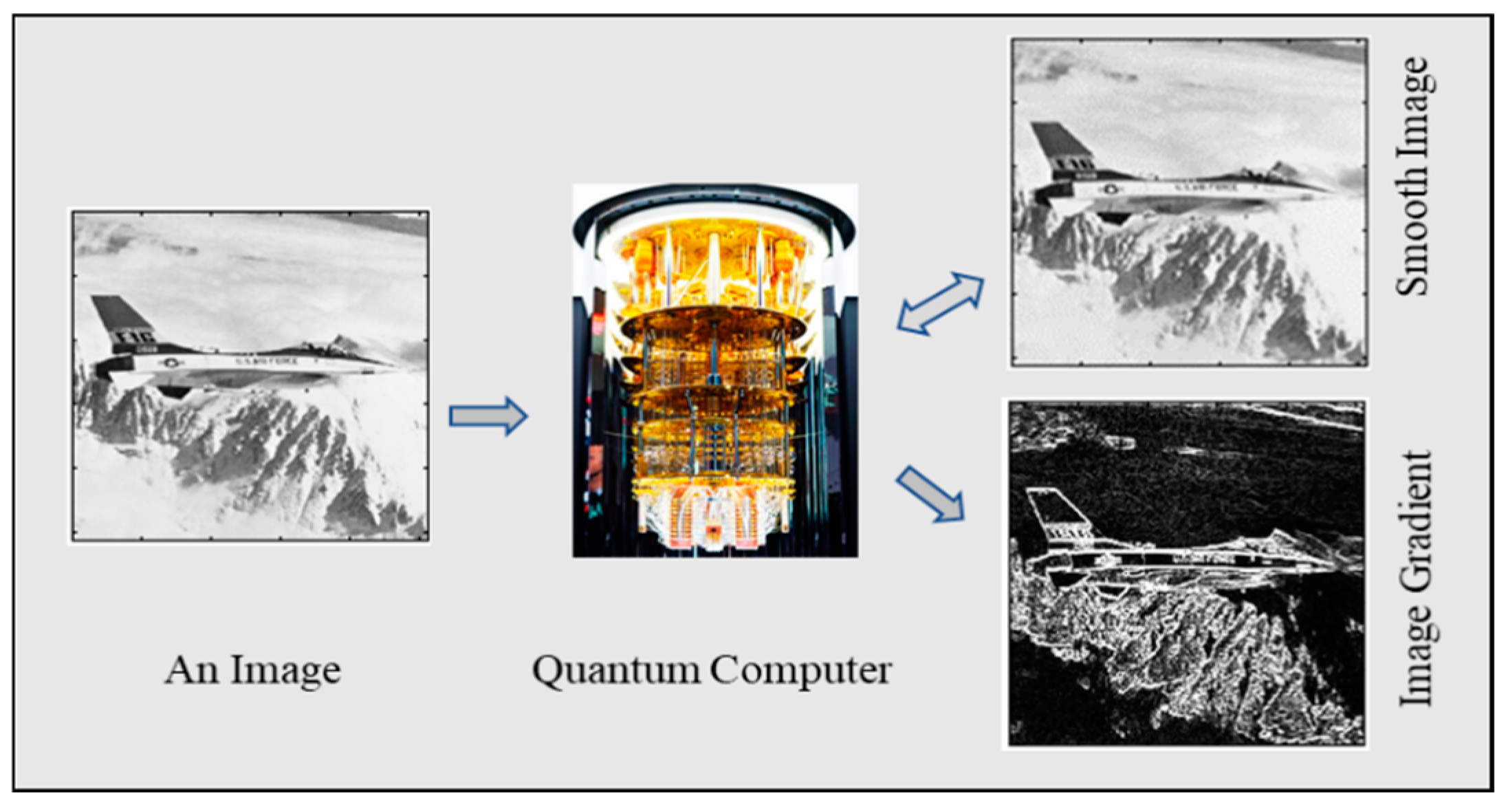
• Simultaneous computation of a few convolutions and gradients (Figure 1).
• Several illustrative examples of quantum algorithms involving two-qubit and three-qubit systems, including edge detection, gradients, and convolution algorithms.

The remainder of the paper is organized as follows. Section 2 describes the fundamental concepts of the qubit and quantum superposition of qubits in the standard computational base of states. Section 3 presents the method of 1D convolution of the signal, which is written in detail for the short-length mask, by using the discrete paired transform. Section 4 and Section 5, provide several examples of the convolution presenting the gradients, including the Sobel gradient operator, are described. The computer simulation of the measurement of results of the proposed method is illustrated through examples with images. Simulations of quantum circuits in Qiskit Version 1.3.2 are discussed in Section 6.

2. Basic Concepts of Qubits

In the theory of quantum computation, qubits (or quantum bits) are described by the superposition of states as elements of a vector subspace, which has a length equal to one [13]. For instance, an individual qubit is described by a superposition

$$\left|\phi ⟩\right.=a_0\left|0⟩\right.+a_1\left|1⟩\right.=\left[\begin{array}{c}{a}_0\\ a_1\end{array}\right],$$

where the coefficients $a$ and $b$ are amplitudes such that ${\left|a_0\right|}^2+{\left|a_1\right|}^2=1$. These coefficients are real or complex numbers. Here, $|0⟩$ and $|1⟩$ denote the computational basis states $\left|0⟩\right.=[\mathrm{1,0}{]}^{\prime }$ and $\left|1⟩\right.=[\mathrm{0,1}{]}^{\prime }$. In this model, it is assumed that the qubit can be measured only once and the measurement results in only one state, $\left|0⟩\right.$ or $\left|1⟩\right.$ with probabilities $p_0={\left|a_0\right|}^2$ or ${p_1=\left|a_1\right|}^2$, respectively. Two-qubit quantum superposition can be written as

$$\left|\phi ⟩\right.=a_0\left|00⟩\right.+a_1\left|01⟩\right.+a_2\left|10⟩\right.+a_3\left|11⟩\right.,$$

with the basis states $\left|00⟩\right.=[\mathrm{1,0},\mathrm{0,0}{]}^{\prime }$, $\left|01⟩\right.=[\mathrm{0,1},\mathrm{0,0}{]}^{\prime }$, $\left|10⟩\right.=[\mathrm{0,0},\mathrm{1,0}{]}^{\prime }$, and $\left|11⟩\right.={\left[\mathrm{0,0},\mathrm{0,1}\right]}^{\prime }.$ The amplitudes $a_k, k=0:3,$ define the probabilities ${\left|a_k\right|}^2$ of measuring the three-qubit in one of the states $\left|k⟩\right.$. The operation $⨂$ of the Kronecker product, or the tensor product, of vectors is used widely in quantum calculations. For instance, we can write the two-qubit basis state $\left|01⟩\right.$ as

$$\left|01⟩\right.=\left|0⟩\right.⨂\left|1⟩=\right.\left[\begin{array}{c}1\\ 0\end{array}\right]⨂\left[\begin{array}{c}0\\ 1\end{array}\right].$$

Let $f$ be a signal ${\{f}_n;n=0:(N-1)\}$ of length $N$, which is considered a power of two, $N=2^r$, $r>1.$ This signal can be represented in the space of $r$-qubit superposition of states as

$$\left|\phi \left(f\right)⟩\right.=\sum _{n=0}^{N-1}{f}_n\left|n⟩.\right.$$

(1)

Here, the basic states

$$\left|n⟩=\left|n_{r-1}\dots n_1{n}_0⟩\right.\right.\triangleq \left|n_{r-1}⟩⨂\right.\dots ⨂\left|n_1⟩\right.⨂\left|n_0⟩\right.$$

are written by using the binary representation of the numbers $n$. All superpositions in quantum computation are probabilistic; that is, their amplitudes form a unit normalized vector. Therefore, the norm of the signal is considered to be 1. Otherwise, the above superposition must be normalized. Thus, the values of the signal are written into the amplitudes of the superposition, and they define the probability of the measurement of the qubits. Many forms exist for quantum representation of 1D and 2D signals (for details, see [29,31]).

For two signals $f$ and $h$ represented in quantum algebra, the linear aperiodic convolution is considered as the $r$-qubit superposition

$$\left|\psi ⟩\right.=\sum _{n=0}^{N-1}{(f \ast h)}_n\left|n⟩\right.=\sum _{n=0}^{N-1}\sum _{k=0}^{N-1}{f}_k{h}_{n-k (\mathrm{m}\mathrm{o}\mathrm{d} N)}\left|n⟩\right..$$

Here, the problem is in calculating this superposition from the superpositions $\left|\phi \left(f\right)⟩\right.$ and $\left|\phi \left(h\right)⟩\right.$, by using only unitary transforms. In quantum computation, all operations on superpositions are described by unitary transforms. As mentioned above, this task is considered unsolvable [28]. Additionally, during the calculation, the same values of the signal are used for the convolution at different points. This fact is not an obstacle in traditional computation when the desired values can be saved and used if needed. However, it is important to mention that no-cloning theorems prohibit the copying of qubits [32].

3. Method of 1-D Quantum Convolution

In this section, we present the method of calculation of short convolutions in a quantum computer. The convolution is an operation over the amplitudes of a quantum superposition of the signal. This method employs two steps.

(a)

First, a quantum representation of the convolution at each point, $\left|n⟩\right.$, is defined. Such a representation may be written in different ways and may lead to different results in calculations. The distinguished property of the proposed method is the fact that, in addition to the given convolution, quantum computing allows for parallel computing of other convolutions as well. Many of these additional convolutions or gradients can also be useful when processing signals. Therefore, both signal and convolution quantum representations, and we are confident of this, need to be analyzed separately for each specific case.

(b)

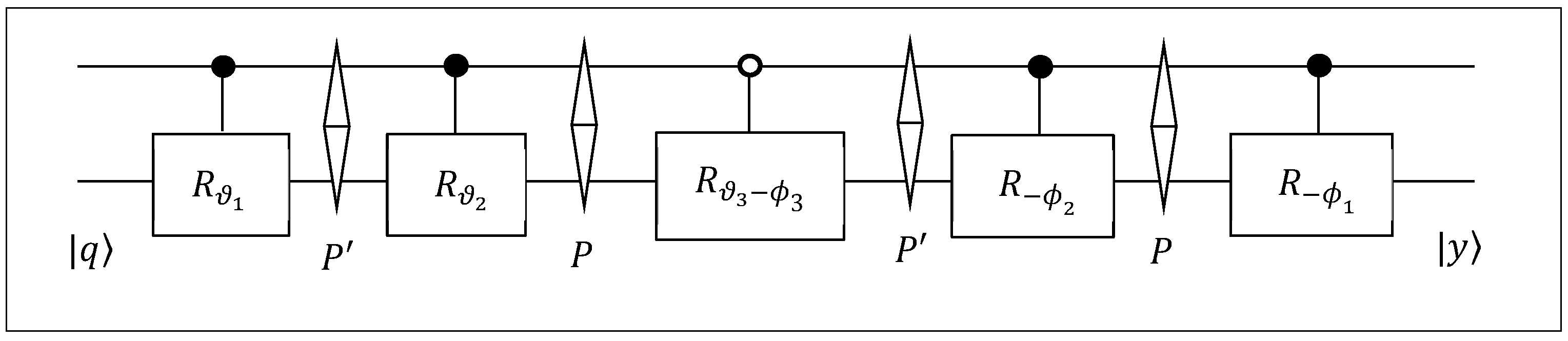
In the second step of the proposed method, the quantum paired transform is applied to parallelize a few convolutions and gradients.

The examples below describe the proposed method.

Convolution Quantum Representation

Let us consider a signal ${\{f}_n;n=0:(N-1)\}$ of length $N=2^r,$ $r>2$, and the following mask of length 4 for the convolution: $M=\left[1 \underset{\_}{2} 2 1\right]$. The underlined number shows the position of the center of the mask, $M\left(0\right)=2$ This signal can be represented by $r$ qubits, when using the representation in Equation (1). We consider that the signal is periodic to simplify the calculation of normalizing coefficients in the quantum representation of signals. The convolution of the signal with this mask is calculated at each point $n$ by

$$y_n={(f \ast M)}_n=f_{n-2}+2f_{n-1}+2f_n+f_{n+1}.$$

(2)

These components of the convolution at point $n$ can be written as the vector $y_n={\left(f_{n-2},2f_{n-1},2f_n,f_{n+1}\right)}^{\prime }.$ We do not yet know how exactly the signal will be recorded on a real quantum computer. However, we believe that the preparation of such amplitudes of the two-qubit $\left|y_n⟩\right.$ will be possible with the help of a classical computer. Thus, we consider the basis state $\left|n⟩\right.$ together with the following two-qubit state superposition:

$$\left|y_n⟩\right.={\displaystyle \frac{1}{A}}\left(f_{n-2}\left|00⟩\right.+2f_{n-1}\left|01⟩\right.+2f_n\left|10⟩\right.+f_{n+1}\left|11⟩\right.\right),$$

(3)

where the coefficient $A=\sqrt{f_{n-2}^2+4f_{n-1}^2+4f_n^2+f_{n+1}^2}$. This two-qubit superposition can be obtained from the two-qubit in the superposition of states

$$\left|q_n⟩\right.={\displaystyle \frac{1}{B}}\left(f_{n-2}\left|00⟩\right.+f_{n-1}\left|01⟩\right.+f_n\left|10⟩\right.+f_{n+1}\left|11⟩\right.\right),$$

by transforming the amplitudes with the diagonal matrix D, as shown

$$D\left(\begin{array}{c}{f}_{n-2}\\ f_{n-1}\\ f_n\\ f_{n+1}\end{array}\right)=\left(\begin{array}{cccc}1& 0& 0& 0\\ 0& 2& 0& 0\\ 0& 0& 2& 0\\ 0& 0& 0& 1\end{array}\right)\left(\begin{array}{c}{f}_{n-2}\\ f_{n-1}\\ f_n\\ f_{n+1}\end{array}\right)=\left(\begin{array}{c}{f}_{n-2}\\ {2f}_{n-1}\\ {2f}_n\\ f_{n+1}\end{array}\right).$$

The coefficient $B=B\left(n\right)=\sqrt{f_{n-2}^2+f_{n-1}^2+f_n^2+f_{n+1}^2}$.

We can note that from point to point, the four numbers in the superpositions of $\left|q_n⟩\right.$ and $\left|q_{n+1}⟩\right.$ change by the cyclic shift and substitution of the last amplitude, as follows:

$$\left(f_{n-2},f_{n-1},f_n,f_{n+1}\right)\to \left(f_{n-1},f_n,f_{n+1},f_{n-2}\right)\to \left(f_{n-1},f_n,f_{n+1},f_{n+2}\right).$$

The matrix $D$ is not unitary, and therefore we consider the quantum algorithm of transforming the two-qubit $\left|q_n⟩\right.$ to $\left|y_n⟩\right.,$

$$T{\displaystyle \frac{1}{B}}\left(\begin{array}{c}{f}_{n-2}\\ f_{n-1}\\ f_n\\ f_{n+1}\end{array}\right)={\displaystyle \frac{1}{A}}\left(\begin{array}{c}{f}_{n-2}\\ {2f}_{n-1}\\ {2f}_n\\ f_{n+1}\end{array}\right).$$

(4)

For that, we can use the concept of the quantum signal-induced transform (QsiPT) [31]. The QsiHT is the quantum analogue of the discrete signal-induced heap transform (DsiHT) [33]. Figure 2 shows the block diagram of the four-point DsiHT generated by a four-point signal $x=(x_0,x_1,x_2,x_3)$. This signal is called the generator of the DsiHT. The output of the transform applied on the generator is the signal $H\left(x\right)=(x_0^{\left(3\right)},\mathrm{0,0},0)$ with the ‘heap’ $x_0^{\left(3\right)}=\pm \sqrt{x_0^2+x_1^2+x_2^2+x_3^2}$. For the signal generator with norm 1, the transform is $H\left(x\right)=\left(\pm \mathrm{1,0},\mathrm{0,0}\right),$ which corresponds to the first basis state $\left|00⟩\right.$ up to sign. Thus, the unitary transform $H$ of the two-qubit superposition of the generator

$$\left|x⟩\right.=x_0\left|00⟩\right.+x_1\left|01⟩\right.+x_2\left|10⟩\right.+x_3\left|11⟩\right.$$

is equal to the state $H\left|x⟩\right.=\pm \left|00⟩\right..$ We denote this transform as $H=H_x$.

Three basic rotations ${R=R}_1$, $R_2,$ and $R_3$ are calculated from the following condition:

$$R\left[\begin{array}{c}a\\ b\end{array}\right]=\left[\begin{array}{rr}\cos \vartheta & -\sin \vartheta \\ \sin \vartheta & \cos \vartheta \end{array}\right]\left[\begin{array}{c}a\\ b\end{array}\right]=\left[\begin{array}{c}{a}^{\left(1\right)}\\ 0\end{array}\right] \mathrm{and} {|a}^{\left(1\right)}|=\sqrt{a^2+b^2}$$

(5)

with the angle $\vartheta =-\arctan \left(b/a\right)$. If $a=0,$ the angle $\vartheta =-\pi /2,$ or $\pi /2.$ The four-point DsiHT collects the energy $‖x‖$ of the generator in one point. The transformation is calculated as follows:

$$\left[\begin{array}{c}{x}_2\\ x_3\end{array}\right]\stackrel{{ R}_{{\vartheta }_1} }{\to }\left[\begin{array}{c}{x}_2^{\left(1\right)}\\ 0\end{array}\right], \left[\begin{array}{c}{x}_1\\ x_2^{\left(1\right)}\end{array}\right]\stackrel{{ R}_{{\vartheta }_2} }{\to }\left[\begin{array}{c}{x}_1^{\left(2\right)}\\ 0\end{array}\right], \left[\begin{array}{c}{x}_0\\ x_1^{\left(2\right)}\end{array}\right]\stackrel{{ R}_{{\vartheta }_3} }{\to }\left[\begin{array}{c}{x}_0^{\left(3\right)}\\ 0\end{array}\right], x_0^{\left(3\right)}=\pm ‖x‖.$$

The set of angles $\{{\vartheta }_1,{\vartheta }_2,{\vartheta }_3\}$ is the angular representation of the generator $x$ in this transformation. On another input z $=(z_0,z_1,z_2,z_3)$, the transform $H_y$ processes the input by the same three rotations, by using the same order, or the path, as

$$\left[\begin{array}{c}{z}_2\\ z_3\end{array}\right]\stackrel{{ R}_{{\vartheta }_1} }{\to }\left[\begin{array}{c}{z}_2^{\left(1\right)}\\ z_3^{\prime }\end{array}\right], \left[\begin{array}{c}{z}_1\\ z_2^{\left(1\right)}\end{array}\right]\stackrel{{ R}_{{\vartheta }_2} }{\to }\left[\begin{array}{c}{z}_1^{\left(2\right)}\\ {z_2}^{\prime }\end{array}\right], \left[\begin{array}{c}{z}_0\\ z_1^{\left(2\right)}\end{array}\right]\stackrel{{ R}_{{\vartheta }_3} }{\to }\left[\begin{array}{c}{z}_0^{\prime }\\ {z_1}^{\prime }\end{array}\right].$$

The DsiHT is a unitary transform. Therefore, $H_x^{\prime }:\left(\mathrm{1,0},\mathrm{0,0}\right)\to \pm x$, or we can write that $H_x^{\prime }\left|00⟩\right.=\pm \left|x⟩\right.$.

The four-point DsiHT, $H_y$, by another generator $y=(y_0,y_1,y_2,y_3)$, works in the same way, that is $H_y\left(y\right)=\left(\pm \mathrm{1,0},\mathrm{0,0}\right),$ or $H\left|y⟩\right.=\pm \left|00⟩\right.$. Therefore, given two four-point vectors $x$ and $y$, we can fulfill the following chain of the transforms, in order to map one vector to another in two steps: (1) $H_x:x\to \pm \left|00⟩\right.$ and (2) $H_y^{\prime }:\pm \left|00⟩\right.\to \left|y⟩\right..$ Thus, the mapping of one two-qubit into another, $x\to y,$ can be accomplished by the transform ${T=H}_y^{\prime }{H}_x$. This transformation allows us to perform the transformation $T$ by maximum five rotation gates. To illustrate this method, we consider the following vectors: ${\mathit{q}}_n={\left(f_{n-2},2f_{n-1},f_n,f_{n+1}\right)}^{\prime }=(\mathrm{3,2},\mathrm{4,1}{)}^{\prime }$ and ${\mathit{y}}_n={\left(f_{n-2},2f_{n-1},2f_n,f_{n+1}\right)}^{\prime }=(\mathrm{3,4},\mathrm{8,1}{)}^{\prime }$, both after the normalization.

Example 1.

Consider two two-qubit superpositions

$$\left|q⟩\right.={\displaystyle \frac{1}{2}}(3\left|00⟩\right.+2\left|01⟩\right.+4\left|10⟩\right.+\left|11⟩\right.)$$

and

$$\left|y⟩\right.={\displaystyle \frac{1}{2}}\left(3\left|00⟩\right.+4\left|01⟩\right.+8\left|10⟩\right.+\left|11⟩\right.\right).$$

The first qubit can be transformed to the initial state $\left|00⟩\right.$, by the following three rotations:

$$H_q=(R_{{\vartheta }_3}\oplus I_2)({1\oplus R}_{{\vartheta }_2}\oplus 1)(I_2\oplus R_{{\vartheta }_1})$$

with the angles $\left\{{\vartheta }_1,{\vartheta }_2,{\vartheta }_3\right\}=\left\{14.0362°, 64.1233°, 56.7891°\right\}.$ Here, the symbol $\oplus$ is used for the operation of direct sum in matrix addition. The circuit for this transformation is shown in Figure 3. The flowchart sorts denote the permutations. The permutations are $P=(\mathrm{0,3},\mathrm{2,1})$ and $P^{\prime }=(\mathrm{0,1},\mathrm{2,3}).$ with the matrices

$$P=\left[\begin{array}{cccc}0& 1& 0& 0\\ 0& 0& 1& 0\\ 0& 0& 0& 1\\ 1& 0& 0& 0\end{array}\right] \mathrm{a}\mathrm{n}\mathrm{d} P^{\prime }=\left[\begin{array}{cccc}0& 0& 0& 1\\ 1& 0& 0& 0\\ 0& 1& 0& 0\\ 0& 0& 1& 0\end{array}\right]$$

Similarly, the QsiHT of the second two-qubit can be transformed to the initial state $\left|00⟩\right.$, by using the angles $\left\{{\varphi }_1,{\varphi }_1,{\varphi }_1\right\}=\left\{7.1250°, 63.6122°, 71.5651°\right\}.$ Therefore, the transfrom $T$ in Equation (4), can be accomplished as $T=H_y^{\prime }{H}_x$, or

$$T=\left(I_2\oplus R_{{-\varphi }_1}\right)\left({1\oplus R}_{-{\varphi }_2}\oplus 1\right)\left(R_{{-\varphi }_3}\oplus I_2\right)\cdot \left(R_{{\vartheta }_3}\oplus I_2\right)\left({1\oplus R}_{{\vartheta }_2}\oplus 1\right)\left(I_2\oplus R_{{\vartheta }_1}\right).$$

We can note that the product $\left(R_{{-\varphi }_3}\oplus I_2\right)\cdot \left(R_{{\vartheta }_3}\oplus I_2\right)=R_{{\vartheta }_3-{\phi }_3}\oplus I_2$. The quantum circuit of the transform $T$ is shown on Figure 4.

The Qiskit Framework is used for simulating this quantum scheme and the remainder of the quantum schemes presented in this paper. The Qiskit Framework is an open-source quantum computing framework developed by IBM. It provides a unified set of tools for creating quantum circuits, simulating their behavior, and running them on real quantum hardware or high-performance simulators. Qiskit’s main functionality includes [34]:

• Circuit Definition and Manipulation: Users can define quantum circuits programmatically, add gates, and easily compose modular, reusable components.
• Simulation Tools: Qiskit’s Aer package allows for efficient simulation of large quantum circuits on classical hardware. This allows for rapid prototyping and debugging before running on an actual quantum device.
• Transpilation and Optimization: Qiskit can automatically optimize and transpile quantum circuits for different backends, ensuring that the circuits are physically realizable on specific quantum chips.

The use of Qiskit in this paper is mostly attributed to its maturity, widespread adoption, and open-source availability. However, any quantum SDK or simulation framework capable of preparing custom quantum states, applying unitary operations, and measuring outcomes could be used to replicate the results.

The results of the quantum simulation using Qiskit for the quantum circuit in Figure 4 are shown in

Table 1. The measured magnitudes for two-qubit superposition $|q⟩=T|q⟩$ by the two-qubit QsiHT.

Basis States	Magnitudes of $\mathit{T}|\mathit{q}⟩$
	Theoretical	500 Shots	1000 Shots	10,000 Shots	100,000 Shots
00	0.3162	0.3193	0.3209	0.3130	0.3167
01	0.4216	0.4449	0.4560	0.4172	0.4201
10	0.8432	0.8330	0.8264	0.8469	0.8434
11	0.1054	0.0774	0.0774	0.1024	0.1079
MSRE	0	6.76 × 10−3	1.04 × 10−2	1.89 × 10−3	3.57 × 10−4

. The mean-square root error (MSRE) of calculations is also given.

The $\left(r+2\right)$-qubit state superposition with all convolution vectors is defined as

$$\left|\phi ⟩\right.=\left|\phi \left(y\right)⟩\right.={\displaystyle \frac{1}{\sqrt{N}}}\sum _{n=0}^{N-1}\left|n⟩\right.\left|y_n⟩\right..$$

(6)

Here, $|n⟩$ denotes the quantum computational basis states of $r$ qubits, and $\left|n⟩\right.\left|y_n⟩\right.=\left|n⟩\right.⨂\left|y_n⟩\right.$. We call such a superposition of the convolution $y_n$ the standard superposition. This superposition requires two additional qubits. The following superposition can also be considered:

$$|\psi ⟩={\displaystyle \frac{1}{C}}\sum _{n=0}^{N-1}\left|n⟩\right.\left(f_{n-2}\left|00⟩\right.+{2f}_{n-1}\left|01⟩\right.+{2f}_n\left|10⟩\right.+f_{n+1}\left|11\right.\right),$$

(7)

where the coefficient $C=\sqrt{6(f_0^2+f_1^2+\dots +f_{N-1}^2)}.$ The difference between these two representations is in the measurement. When measuring the first $r$ qubits $\left|n⟩\right.$ in the superposition in Equation (6), we obtain two qubits in a superposition of states $\left|y_n⟩\right.$ with probability equal to $1/N$. The possibility of measuring the same two qubits in the superposition in Equation (7) equals $1/C^2.$ Note that $\left|y_n⟩\right.$ are the superpositions of two qubits at points $n$, and our goal is to calculate the values $y_n$ of the convolution after processing $(r+2)$ qubits being in the superposition $\left|\phi ⟩\right.$ or $\left|\psi ⟩\right.$.

Now, we process $\left|y_n⟩\right.$ in Equation (3) by the two-qubit quantum paired transform (QPT). In the matrix form, the four-point discrete paired transform (DPT), ${\chi }_4^{\prime }$, of a signal ${x=\{x}_0,x_1,x_2,x_3\}$ is calculated as [33]

$${\chi }_4^{\prime }[x]=\left[\begin{array}{cccc}1& 0& -1& 0\\ 0& 1& 0& -1\\ 1& -1& 1& -1\\ 1& 1& 1& 1\end{array}\right]\left[\begin{array}{c}{x}_0\\ x_1\\ x_2\\ x_3\end{array}\right].$$

(8)

The $4\times 4$ matrix with determinant 8 in this equation is considered the orthogonal (unitary) matrix after multiplying by the diagonal matrix [33],

$$\left[{\chi }_4^{\prime }\right]=\left[\begin{array}{cccc}{\displaystyle \frac{1}{\sqrt{2}}}& 0& 0& 0\\ 0& {\displaystyle \frac{1}{\sqrt{2}}}& 0& 0\\ 0& 0& {\displaystyle \frac{1}{2}}& 0\\ 0& 0& 0& {\displaystyle \frac{1}{2}}\end{array}\right]\left[\begin{array}{cccc}1& 0& -1& 0\\ 0& 1& 0& -1\\ 1& -1& 1& -1\\ 1& 1& 1& 1\end{array}\right]=\left[\begin{array}{cccc}{\displaystyle \frac{1}{\sqrt{2}}}& 0& -{\displaystyle \frac{1}{\sqrt{2}}}& 0\\ 0& {\displaystyle \frac{1}{\sqrt{2}}}& 0& -{\displaystyle \frac{1}{\sqrt{2}}}\\ {\displaystyle \frac{1}{2}}& -{\displaystyle \frac{1}{2}}& {\displaystyle \frac{1}{2}}& -{\displaystyle \frac{1}{2}}\\ {\displaystyle \frac{1}{2}}& {\displaystyle \frac{1}{2}}& {\displaystyle \frac{1}{2}}& {\displaystyle \frac{1}{2}}\end{array}\right].$$

(9)

The $2\times 2$ operation of the butterfly for this transform is described by the matrix

$${\mathit{A}}_2={\displaystyle \frac{1}{\sqrt{2}}}\left[\begin{array}{cc}1& -1\\ 1& 1\end{array}\right]=\left[\begin{array}{cc}0& 1\\ 1& 0\end{array}\right]{\displaystyle \frac{1}{\sqrt{2}}}\left[\begin{array}{cc}1& 1\\ 1& -1\end{array}\right]=\mathit{X}\mathit{H},$$

where X is the NOT gate and H is the 2 × 2 Hadamard matrix. The quantum circuit for the two-qubit DPT is shown in Figure 5 [24]. The input in this circuit is the two-qubit state superposition

$$|{\phi }_2⟩={\displaystyle \frac{1}{A}}\sum _{n=0}^3{x}_n|n⟩, A=\sqrt{x_0^2+x_1^2+x_3^2+x_3^2},$$

where $|n⟩$ denotes the basis state. The bullet on the line denotes the control qubit.

For simplicity of calculations, we consider the four-point DPT, as given in Equation (8), that is, the transform defined by the matrix with the integer-valued coefficients. The paired transform of the vector ${\mathit{y}}_n$ at point $n$ is calculated by

$$\left[\begin{array}{cccc}1& 0& -1& 0\\ 0& 1& 0& -1\\ 1& -1& 1& -1\\ 1& 1& 1& 1\end{array}\right]\left[\begin{array}{r}{f}_{n-2}\\ {2f}_{n-1}\\ {2f}_n\\ f_{n+1}\end{array}\right]=\left[\begin{array}{c}{f}_{n-2}-2f_n\\ {2f}_{n-1}-f_{n+1}\\ f_{n-2}-2f_{n-1}+{2f}_n-f_{n+1}\\ f_{n-2}+2f_{n-1}+{2f}_n+f_{n+1}\end{array}\right].$$

The result of the transformation is the two-qubit

$$\left|{{\chi }_4^{\prime }(y}_n)⟩=c_0\right|00⟩+c_1\left|01⟩+c_2\right|10⟩+c_3|11⟩$$

(10)

with the following amplitudes of the basic states: $c_0=f_{n-2}-2f_n, c_1={2f}_{n-1}-f_{n+1}; c_2=f_{n-2}-2f_{n-1}+{2f}_n-f_{n+1};$ and $c_3=f_{n-2}+2f_{n-1}+{2f}_n+f_{n+1}.$ These amplitudes should be normalized by the coefficient $\sqrt{c_0^2+c_1^2+c_2^2+c_3^2}$.

The coefficient $c_1$ can be written as $c_1={f_{n-1}+(f}_{n-1}-f_{n+1})$, which describes the shifted signal $f_{n-1}$ plus the gradient $G({f_{n-1})=(f}_{n-1}-f_{n+1})$ with the mask [1 0 −1]. We can note that (up to the constant 6) the amplitude $c_3$ is the value of the convolution, $y_n$, with the mask [1 2 2 1]/6,

$$c_3=y_n={\displaystyle \frac{1}{6}}\left[\begin{array}{cccc}1& 2& 2& 1\end{array}\right]\left[\begin{array}{c}{f}_{n-2}\\ f_{n-1}\\ f_n\\ f_{n+1}\end{array}\right]$$

(11)

The amplitude $c_2$ is the value of the convolution, which is described by the mask [−1 2 −2 1]/3 and it represents the 4-level gradient operator,

$$c_2=G_n\left(f\right)={\displaystyle \frac{1}{3}}\left[\begin{array}{cccc}1& -2& 2& -1\end{array}\right]\left[\begin{array}{c}{f}_{n-2}\\ f_{n-1}\\ f_n\\ f_{n+1}\end{array}\right]$$

(12)

Figure 6 shows the circuit element for processing two-qubit $\left|y_n⟩\right.$, by the two-qubit QPT. Thus, the paired transformation allows for the parallel computation of two different convolutions, one of which is the gradient operation.

4. Gradient Operators and Numerical Simulations

In this section, we describe examples that illustrate the presented method of convolution. For example, we consider the quantum representation for the gradient with the mask $M=\left[1-\underset{\_}{2} 1\right]/2$. At each point $n$, the gradient of the signal, or the convolution of the signal with this mask, is calculated by

$$G_n\left(f\right)={(f\ast M)}_n=\left[f_{n-1}-2f_n+f_{n+1}\right]/2.$$

(13)

This operation can be expressed as

$$G_n\left(f\right)=\left[{(f}_{n-1}-f_n)+{(f}_{n+1}-f_n)\right]/2.$$

Therefore, we define the following two-qubit state superposition at point $n$:

$$\left|y_n⟩\right.={\displaystyle \frac{1}{A}}\left(f_{n-1}\left|00⟩\right.-f_n\left|01⟩\right.+f_{n+1}\left|10⟩\right.-f_n\left|11⟩\right.\right)$$

(14)

and the vector $y_n={\left(f_{n-2},-f_n,f_{n+1},f_n\right)}^{\prime }.$ The coefficient $A=A\left(n\right)=\sqrt{f_{n-1}^2+2f_n^2+f_{n+1}^2}$. The $(r+2)$-qubit state superposition for the gradient of the signal is considered in the standard form (Equation (6)).

The following superposition can also be used:

$$\left|\psi ⟩\right.=\left|\psi \left(y\right)⟩\right.={\displaystyle \frac{1}{C}}\sum _{n=0}^{N-1}\left|n⟩\right.\left|y_n⟩=\right.{\displaystyle \frac{1}{C}}\sum _{n=0}^{N-1}\left|n⟩\right.\left|\left(f_{n-1}\left|00⟩\right.-f_n\left|01⟩\right.+f_{n+1}\left|10⟩\right.-f_n\left|11⟩\right.\right).\right.$$

The coefficient $C=2\sqrt{(f_0^2+f_1^2+\dots +f_{N-1}^2)}$.

The four-point DPT of the amplitudes of $\left|y_n⟩\right.$ is calculated by

$$\left[\begin{array}{cccc}1& 0& -1& 0\\ 0& 1& 0& -1\\ 1& -1& 1& -1\\ 1& 1& 1& 1\end{array}\right]\left[\begin{array}{r}{f}_{n-1}\\ {-f}_n\\ f_{n+1}\\ {-f}_n\end{array}\right]=\left[\begin{array}{c}{f}_{n-1}-f_{n+1}\\ 0\\ f_{n-1}+{2f}_n+f_{n+1}\\ f_{n-1}-{2f}_n+f_{n+1}\end{array}\right].$$

(15)

Thus, the two-qubit paired transform on the input $|y_n⟩$ is the two-qubit superposition

$$\left|{{\chi }_4^{\prime }(y}_n)⟩=c_0\right|00⟩+c_1\left|01⟩+c_2\right|10⟩+c_3|11⟩$$

(16)

with the following amplitudes of the states: $c_0=f_{n-1}-f_{n+1};c_1=0,c_2=f_{n-1}+{2f}_n+f_{n+1};$ and $c_3=f_{n-1}-2f_n+f_{n+1}.$ These amplitudes of states should be normalized by the coefficient $A=\sqrt{c_0^2+c_2^2+c_3^2.}$ Up to the factor 2, the amplitude $c_3$ is the value of the gradient $G_n\left(f\right)$ at point $n$,

$$c_3=c_3(n)=G_n\left(f\right)={\displaystyle \frac{1}{2}}\left[\begin{array}{ccc}1& -2& 1\end{array}\right]\left[\begin{array}{c}{f}_{n-1}\\ f_n\\ f_{n+1}\end{array}\right].$$

(17)

Up to factor of 4, the amplitude $c_2$ equals the convolution of the signal at point $n$, when the mask is [1 2 1]/4,

$$c_2=c_2\left(n\right)={\displaystyle \frac{1}{4}}\left[\begin{array}{ccc}1& 2& 1\end{array}\right]\left[\begin{array}{c}{f}_{n-1}\\ f_n\\ f_{n+1}\end{array}\right].$$

(18)

Thus, in this example also, the two-qubit paired transform also allows for the parallel calculation of the convolution and the gradient of the signal. It should be noted that, for the parallel calculation of these two convolutions with a mask of length 3, four amplitudes of two-qubit in Equation (14) were determined in a certain way.

As an example, Figure 7 shows the grayscale image ‘house’ of size 256 × 256 pixels in part (a). The images composed by $c_0$(n), $c_1$(n), and $c_3$(n) coefficients are shown in parts (b), (c), and (d), respectively.

Additionally, we consider the above operations over each row of length 512 of the image ‘jetplane.jpg’ of size 512 × 512 pixels in Figure 8a. The images composed by $c_0$(n), $c_2$(n), and $c_3$(n) coefficients are shown in parts (b–d), respectively. The images in parts (b,d) are gradient images, and the image in part (c) was smoothed along the $X$ axis.

At each pixel $n$, the two-qubit superposition in Equation (16) is $|{{\chi }_4^{\prime }(y}_n)⟩={(f}_{n-1}-f_{n+1})|00⟩+c_2\left|10⟩+c_3\right|11⟩.$ Therefore, if we measure the first qubit in the state $\left|0⟩\right.,$ we obtain the image shown in Figure 8b. Figure 9 shows the quantum circuit of two-qubit QPT of the two-qubit ${{|\chi }_4^{\prime }(y}_n)⟩$ with the result of the measurement, $M=0$, for the ‘jetplane’ image.

We can model the process of measurements of all $(r+2)$ qubits $\left|\psi ⟩\right.$ for this image, and consider the probability of measuring the two-qubit ${|y}_n⟩$ in basis states $\left|00⟩\right.,$ $\left|10⟩,\right.$ and $\left|11⟩\right.$ according to the coefficients ${|c}_0{|}^2$, ${|c}_2{|}^2$, and ${|c}_3{|}^2$. Figure 10a illustrates this random model of measurement. For each point $n$, the unit interval $\left[\mathrm{0,1}\right]$ is partitioned by three parts with the lengths equal to ${|c}_0{|}^2$, ${|c}_2{|}^2$, and ${|c}_3{|}^2$, respectively. These parts can also be considered in the increasing order of their lengths. Then the random number $x$ is generated in this interval. If the number $x$ falls, for instance, into the second part (as shown in the figure), then the measured value of the two-qubit superposition ${|y}_n⟩$ is considered to be $c_2.$ Otherwise, if $x\in [0, c_0^2)$, the measured value is $c_0,$ and if $x\in [c_3^2, 1]$, the measured value is $c_3$. The result of such a simulation on a classical computer is shown in Figure 10b. For each row of the image, at each point $n\in \{\mathrm{1,\; 2}, \dots , 512\}$, the value of row-signal was taken randomly from the corresponding set of amplitudes ${\{c}_0\left(n\right), c_2\left(n\right), c_3\left(n\right)\}$. The edge points can be extracted by the threshold operation of the quantum bit sequence [11].

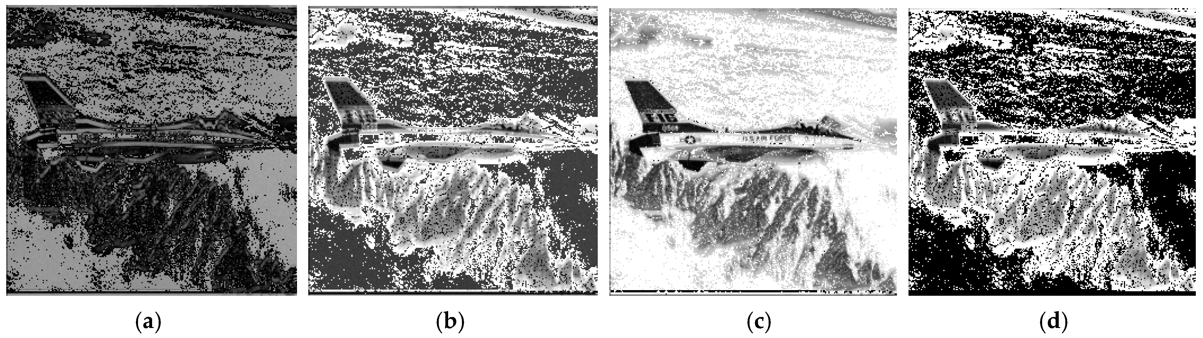
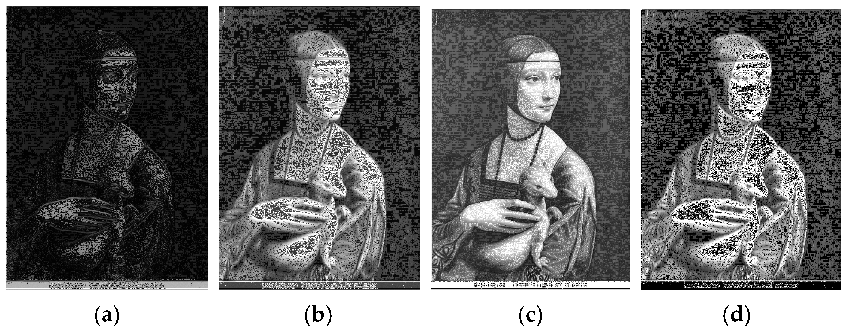
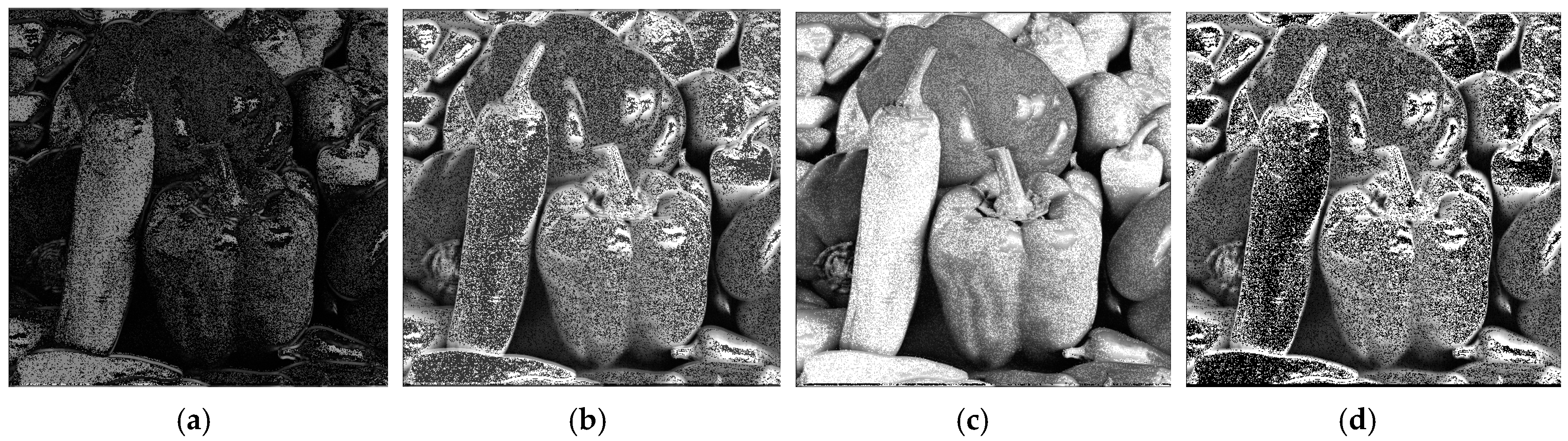
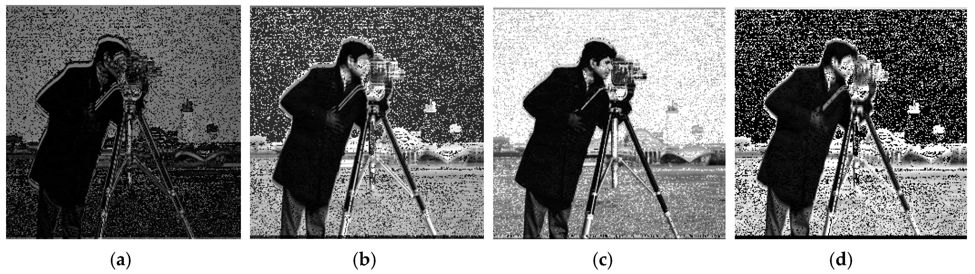
5. Numerical Simulations: Sobel Gradient Operators

This section focuses on the conventional image processing edge detection task, which is the perception of boundaries (intensity changes) between two neighboring regions. The brain uses this task: It has been shown that the brain processes visual information by responding to lines and edges with different neurons, which is an essential step in many pattern recognition tasks [35]. Edge detection methods employ an image gradient by applying different types of filtering masks. We consider the quantum representation of the 5-level Sobel gradient operator [5] with the mask $M=$ [−1 −2 0 2 1]/3. The gradient of the signal, or the convolution of the signal with this mask, is calculated at each point $n$ by

$$G_5\left(n\right)={(f \ast M)}_n={\displaystyle \frac{\left[f_{n-2}+{2f}_{n-1}-2f_{n+1}-f_{n+2}\right]}{3}}.$$

(19)

This operation can be written as the sum with 8 terms.

$$\begin{gathered} G_5\left(n\right)={\displaystyle \frac{1}{3}}\left[{(f}_{n-2}-f_n)+{2(f}_{n-1}-f_n)+{2(f}_n-f_{n+1})+{(f}_n-f_{n+2})\right] \\ ={\displaystyle \frac{1}{3}}\left[{(f}_{n-2}-f_n)+{2(f}_{n-1}-f_n)-{2(f}_{n+1}-f_n)-{(f}_{n+2}-f_n)\right]. \end{gathered}$$

5.1. Three-Qubit Gradient Representation

We can consider the following quantum representation of the three-qubit for the convolution at point $n$:

$$\left|y_n⟩\right.={\displaystyle \frac{1}{A}}\left(f_{n-2}\left|0⟩\right.-f_n\left|1⟩\right.+2f_{n-1}\left|2⟩\right.-{2f}_n\left|3⟩\right.+2f_n\left|4⟩-2f_{n+1}\left|5⟩\right.\right.+f_n\left|6⟩\right.-f_{n+2}\left|7⟩\right.\right).$$

Here, the coefficient

$$A=\sqrt{f_{n-2}^2+{4f}_{n-1}^2+10f_n^2+{4f}_{n+1}^2+f_{n+2}^2}.$$

The corresponding 8-dimensional vector is

$${\mathit{y}}_n={\left(f_{n-2},-f_n,{2f}_{n-1},-{2f}_n,2f_n,-{2f}_{n+1},f_n,-f_{n+2}\right)}^{\prime }.$$

The $(r+3)$-qubit state superposition for the gradient of the signal is considered in standard form (3). We can also use the following superposition:

$$\left|\psi ⟩\right.={\displaystyle \frac{1}{C}}\sum _{n=0}^{N-1}\left|n⟩\right.\left|\left(f_{n-2}\left|0⟩\right.-f_n\left|1⟩\right.+2f_{n-1}\left|2⟩\right.-{2f}_n\left|3⟩+\right.+2f_n\left|4⟩-2f_{n+1}\left|5⟩\right.\right.+f_n\left|6⟩\right.-f_{n+2}\left|7⟩\right.\right) \right.$$

with the coefficient $C=\sqrt{20(f_0^2+f_1^2+\dots +f_{N-1}^2)}$.

The eight-point discrete paired transform is defined by the following unitary matrix [33]:

$$\begin{gathered} \left[{\chi }_8^{\prime }\right]=\mathrm{d}\mathrm{i}\mathrm{a}\mathrm{g}\left\{{\displaystyle \frac{1}{\sqrt{2}}},{\displaystyle \frac{1}{\sqrt{2}}},{\displaystyle \frac{1}{\sqrt{2}}},{\displaystyle \frac{1}{\sqrt{2}}},{\displaystyle \frac{1}{2}},{\displaystyle \frac{1}{2}},{\displaystyle \frac{1}{\sqrt{8}}},{\displaystyle \frac{1}{\sqrt{8}}}\right\}\times \\ \left[\begin{array}{cccccccc}1& 0& 0& 0& -1& 0& 0& 0\\ 0& 1& 0& 0& 0& -1& 0& 0\\ 0& 0& 1& 0& 0& 0& -1& 0\\ 0& 0& 0& 1& 0& 0& 0& -1\\ 1& 0& -1& 0& 1& 0& -1& 0\\ 0& 1& 0& -1& 0& 1& 0& -1\\ 1& -1& 1& -1& 1& -1& 1& -1\\ 1& 1& 1& 1& 1& 1& 1& 1\end{array}\right]. \end{gathered}$$

For simplicity of calculations, we consider the eight-point discrete paired transform, ${\chi }_8^{\prime }$, which has the above matrix with the integer-valued coefficients 0 and $\pm 1.$ The transform over amplitudes of the three-qubit $\left|y_n⟩\right.$ is equal to

$$\begin{gathered} {\chi }_8^{\prime }\left[y_n\right]=\left[\begin{array}{cccccccc}1& 0& 0& 0& -1& 0& 0& 0\\ 0& 1& 0& 0& 0& -1& 0& 0\\ 0& 0& 1& 0& 0& 0& -1& 0\\ 0& 0& 0& 1& 0& 0& 0& -1\\ 1& 0& -1& 0& 1& 0& -1& 0\\ 0& 1& 0& -1& 0& 1& 0& -1\\ 1& -1& 1& -1& 1& -1& 1& -1\\ 1& 1& 1& 1& 1& 1& 1& 1\end{array}\right]\left[\begin{array}{c}{f}_{n-2}\\ {-f}_n\\ 2f_{n-1}\\ {-2f}_n\\ {2f}_n\\ {-2f}_{n+1}\\ f_n\\ -f_{n+2}\end{array}\right] \\ =\left[\begin{array}{c}{{-2f}_n+f}_{n-2}\\ -f_n{+2f}_{n+1}\\ -f_n+2f_{n-1}\\ {-2f}_n+f_{n+2}\\ {f_{n-2}-2f}_{n-1}+f_n\\ f_n{-2f}_{n+1}+f_{n+2}\\ {f_{n-2}+2f}_{n-1}+{6f}_n+{2f}_{n+1}+f_{n+2}\\ {f_{n-2}+2f}_{n-1}-{2f}_{n+1}-f_{n+2}\end{array}\right]. \end{gathered}$$

(20)

One can see that the last four components of the paired transform are the convolutions of the signal with the masks [1 −2 1], [1 −2 1], [1 2 6 2 1], and [ −1 −2 0 2 1]. The first four outputs describe the signal plus gradients. Indeed,

$$c_0={{-2f}_n+f}_{n-2}=-\left[{f_n+(f_n-f}_{n-2}\right)],$$

$$c_1={{-f}_n+2f}_{n+1}={f_{n+1}+(f_{n+1}-f}_n),$$

$$c_2={{-f}_n+2f}_{n-1}={f_{n-1}+(f_{n-1}-f}_n),$$

$$c_3={{-2f}_n+f}_{n+2}=-\left[{f_n+(f_n-f}_{n+2}\right)].$$

The quantum circuit for computing the three-qubit QPT is shown in Figure 11 (for more details see [24]). The transformation of the input $|y_n⟩$ is the following three-qubit state superposition:

$$\left|{{\chi }_8^{\prime }(y}_n)\right.⟩={\displaystyle \frac{1}{C}}\sum _{k=0}^7{c}_k|k⟩.$$

Thus, when the first qubit is in state $\left|1⟩,\right.$ the transformation coefficients $c_4, c_5$, $c_6$, and $c_7$, or the amplitudes of the new superposition of states

$${\left|{{\chi }_8^{\prime }(y}_n)\right.⟩}_1={\displaystyle \frac{1}{C_1}}\left(c_4\left|00⟩+c_5\right|01⟩+c_6|10⟩+c_7|11⟩\right),$$

describe the different convolutions and gradients. Here, the normalizing coefficient is equal to $C_1=\sqrt{c_4^2+c_5^2+c_6^2+c_7^2}$.

Figure 11. The quantum circuit for the three-qubit QPT.

Figure 11. The quantum circuit for the three-qubit QPT.

Considering the 2-level Sobel gradient

$$G_2\left(n\right)={\displaystyle \frac{1}{2}}\left[\begin{array}{ccc}1& -2& 1\end{array}\right]\left[\begin{array}{c}{f}_{n-1}\\ f_n\\ f_{n+1}\end{array}\right],$$

we can write that the amplitudes $c_4$ and $c_5$ are the values of this gradient, which are calculated at two points, $(n-1)$ and $(n+1)$, that is,

$$c_4={\displaystyle \frac{1}{2}}\left[\begin{array}{ccc}1& -2& 1\end{array}\right]\left[\begin{array}{c}{f}_{n-2}\\ f_{n-1}\\ f_n\end{array}\right]=G_2\left(n-1\right),$$

(21)

$$c_5={\displaystyle \frac{1}{2}}\left[\begin{array}{ccc}1& -2& 1\end{array}\right]\left[\begin{array}{c}{f}_n\\ f_{n+1}\\ f_{n+2}\end{array}\right]=G_2\left(n+1\right).$$

The amplitude $c_6$ describes the convolution of the signal at point $n$, when the mask is [1 2 6 2 1]/12,

$$c_6=C\left(n\right)={\displaystyle \frac{1}{12}}\left[\begin{array}{ccccc}1& 2& 6& 2& 1\end{array}\right]\left[\begin{array}{c}{f}_{n-2}\\ f_{n-1}\\ f_n\\ f_{n+1}\\ f_{n+2}\end{array}\right].$$

(22)

The last amplitude $c_7$ corresponds to the 5-level Sobel gradient of the signal at point $n$,

$$c_7=G_5\left(n\right)={\displaystyle \frac{1}{3}}\left[\begin{array}{ccccc}1& 2& 0& -2& -1\end{array}\right]\left[\begin{array}{c}{f}_{n-2}\\ f_{n-1}\\ f_n\\ f_{n+1}\\ f_{n+2}\end{array}\right].$$

(23)

We can see from the above equations that the measurement of the first and second qubits in the state $\left|1⟩\right.$ results in the smooth operation $c_{110}=c_4=C\left(n\right)$ and the 5-level Sobel gradient $c_{111}=c_7=G_5\left(n\right)$. If the first and third qubits are in the state $\left|1⟩\right.$, the result of the measurement is two Sobel gradients $c_{101}=c_5=G_2\left(n+1\right)$ and the 5-level Sobel gradient $c_{111}=G_5\left(n\right)$.

Figure 12 shows the circuit element for processing the two-qubit $\left|y_n⟩\right.$, by the three-qubit DPT of the input three-qubit $|y_n⟩$. This transformation allows for parallel computing three different convolutions, one of which is the 5-level Sobel gradient transform. The two-level gradient $G_2$ is calculated in two points, $(n-1)$ and $(n+1)$.

5.2. Three-Qubit Gradient Quantum Representation

Now, we consider another quantum representation of the three-qubit for the convolution at point $n$,

$$\left|y_n⟩\right.={\displaystyle \frac{1}{A}}\left(f_{n-2}\left|0⟩\right.-f_n\left|1⟩\right.+2f_{n-1}\left|2⟩\right.-{2f}_n\left|3⟩\right.-2f_{n+1}\left|4⟩\right.+2f_n\left|5⟩\right.-f_{n+2}\left|6⟩+f_n\left|7⟩\right.\right.\right)$$

(24)

The corresponding 8-dimensional vector is

$${\mathit{y}}_n={\left(f_{n-2},-f_n,{2f}_{n-1},-{2f}_n,-{2f}_{n+1},2f_n,-f_{n+2},f_n\right)}^{\prime }.$$

The $(r+3)$-qubit state superposition for the gradient of the signal can be written as

$$\left|\phi ⟩\right.=\left|\phi \left(y\right)⟩\right.={\displaystyle \frac{1}{\sqrt{N}}}\sum _{n=0}^{N-1}\left|n⟩\right.\left|y_n⟩\right..$$

The following superposition of states can also be considered:

$$\left|\psi ⟩\right.={\displaystyle \frac{1}{C}}\sum _{n=0}^{N-1}\left|n⟩\right.\left|\left(f_{n-2}\left|0⟩\right.-f_n\left|1⟩\right.+2f_{n-1}\left|2⟩\right.-{2f}_n\left|3⟩\right.-2f_{n+1}\left|4⟩\right.+2f_n\left|5⟩\right.-f_{n+2}\left|6⟩+f_n\left|7⟩\right.\right.\right).\right.$$

Thus, if the first $r$ qubits are in the basis state $\left|n⟩\right.$, the next two qubits will be in the three-qubit superposition $\left|y_n⟩\right.$. The eight-point discrete paired transform, ${\chi }_8^{\prime }$, over the amplitudes of two-qubit $\left|y_n⟩\right.$ equals to

$${\chi }_8^{\prime }\left[{\mathit{y}}_n\right]={\chi }_8^{\prime }\left[\begin{array}{c}{f}_{n-2}\\ {-f}_n\\ 2f_{n-1}\\ {-2f}_n\\ {-2f}_{n+1}\\ {2f}_n\\ -f_{n+2}\\ f_n\end{array}\right]=\left[\begin{array}{c}{f}_{n-2}+{2f}_{n+1}\\ -{3f}_n\\ 2f_{n-1}+f_{n+2}\\ {-3f}_n\\ {f_{n-2}-2f}_{n-1}-{2f}_{n+1}+f_{n+2}\\ {2f}_n\\ {f_{n-2}+2f}_{n-1}-{2f}_{n+1}-f_{n+2}\\ {f_{n-2}+2f}_{n-1}-{2f}_{n+1}-f_{n+2}\end{array}\right].$$

Thus, the three-qubit QPT of the input qubit $|y_n⟩$ is the following three-qubit state superposition (up to a normalizing coefficient):

$$\left|{{\chi }_8^{\prime }(y}_n)\right.⟩=\sum _{k=0}^7{c}_k|k⟩.$$

(25)

Two amplitudes $c_6$ and $c_7$ describe the same convolution, namely, the 5-level Sobel gradient at point $n$,

$$c_6=c_7=G_5\left(n\right)={\displaystyle \frac{1}{3}}\left[\begin{array}{ccccc}1& 2& 0& -2& -1\end{array}\right]\left[\begin{array}{c}{f}_{n-2}\\ f_{n-1}\\ f_n\\ f_{n+1}\\ f_{n+2}\end{array}\right].$$

Therefore, if the first two qubits in the three-qubit superposition $\left|{{\chi }_8^{\prime }(y}_n)\right.⟩$ are in state $\left|1⟩\right.$ each, the measurement will result in the 5-level Sobel gradient at point $n$.

Up to the sign, the amplitude $c_4$ describes the convolution with average and gradient operations,

$$c_4={\displaystyle \frac{1}{2}}\left[\begin{array}{ccccc}-1& 2& 0& 2& -1\end{array}\right]\left[\begin{array}{c}{f}_{n-2}\\ f_{n-1}\\ f_n\\ f_{n+1}\\ f_{n+2}\end{array}\right]={\displaystyle \frac{1}{2}}\left(f_{n-1}+f_{n+1}\right)+{\displaystyle \frac{1}{2}}\left[\begin{array}{ccccc}-1& 1& 0& 1& -1\end{array}\right]\left[\begin{array}{c}{f}_{n-2}\\ f_{n-1}\\ f_n\\ f_{n+1}\\ f_{n+2}\end{array}\right].$$

(26)

One can see that the representations of the convolution in parts A and B are different. Although the 5-level Sobel gradient was used in both representations, other convolutions and signal gradients are also calculated.

5.3. Other Gradient Operators

The proposed method of quantum representation of short convolutions can also be used for other gradient operators [5,6]. For example, we consider the gradient operator with the mask $M=\left[1 1-\underset{\_}{4} 1 1\right]/4$. The gradient of the signal $f_n$ at each point $n$ is calculated by

$$G_5\left(n\right)={(f \ast M)}_n=\left[f_{n-2}+f_{n-1}-4f_n+f_{n+1}+f_{n+2}\right]/4.$$

We consider the following quantum representation of the three-qubit for the convolution at point $n$:

$$\left|y_n⟩\right.={\displaystyle \frac{1}{A}}\left(f_{n-2}\left|0⟩\right.-f_n\left|1⟩\right.+f_{n-1}\left|2⟩\right.-f_n\left|3⟩\right.+f_{n+1}\left|4⟩-f_n\left|5⟩\right.\right.+f_{n+2}\left|6⟩\right.-f_n\left|7⟩\right.\right).$$

Here, the coefficient

$$A=A\left(n\right)=\sqrt{f_{n-2}^2+f_{n-1}^2+4f_n^2+f_{n+1}^2+f_{n+2}^2}.$$

Therefore, the corresponding 8D vector at point $n$ is defined as

$${\mathit{y}}_n={\left(f_{n-2},-f_n,f_{n-1},-f_n,f_{n+1},-f_n,f_{n+2},{-f}_n\right)}^{\prime }.$$

The eight-point DPT of the convolution vector ${\mathit{y}}_n$ equals

$${\chi }_8^{\prime }\left[{\mathit{y}}_n\right]={\chi }_8^{\prime }\left[\begin{array}{c}{f}_{n-2}\\ {-f}_n\\ f_{n-1}\\ {-f}_n\\ f_{n+1}\\ {-f}_n\\ f_{n+2}\\ -f_n\end{array}\right]=\left[\begin{array}{c}{f}_{n-2}-f_{n+1}\\ 0\\ f_{n-1}-f_{n+2}\\ 0\\ {f_{n-2}-f}_{n-1}+f_{n+1}-f_{n+2}\\ 0\\ {f_{n-2}+f}_{n-1}+4f_n+f_{n+1}+f_{n+2}\\ {f_{n-2}+f}_{n-1}-{4f}_n+f_{n+1}+f_{n+2}\end{array}\right].$$

Therefore, the three-qubit QPT of the input $|y_n⟩$ is the three-qubit state superposition

$$\left|{{\chi }_8^{\prime }(y}_n)\right.⟩={\displaystyle \frac{1}{C}}\sum _{k=0}^7{c}_k|k⟩$$

(27)

with the amplitudes $c_1=c_3=c_5=0.$ The other five amplitudes represent a convolution and three gradient operations at point $n$. Indeed, $c_0=c_0\left(n\right)=f_{n-2}-f_{n+1}$ $c_2=c_2\left(n\right)=f_{n-1}-f_{n+2}=c_0\left(n+1\right)$, and (up to the factors 2, 8, and 2, respectively), the other amplitudes are

$$c_4=c_4\left(n\right)={\displaystyle \frac{1}{2}}\left[\begin{array}{ccccc}1& -1& 0& 1& -1\end{array}\right]\left[\begin{array}{c}{f}_{n-2}\\ f_{n-1}\\ f_n\\ f_{n+1}\\ f_{n+2}\end{array}\right],$$

$$c_6=c_6\left(n\right)={\displaystyle \frac{1}{8}}\left[\begin{array}{ccccc}1& 1& 4& 1& 1\end{array}\right]\left[\begin{array}{c}{f}_{n-2}\\ f_{n-1}\\ f_n\\ f_{n+1}\\ f_{n+2}\end{array}\right],$$

$$c_7=c_7\left(n\right)={\displaystyle \frac{1}{2}}\left[\begin{array}{ccccc}1& 1& -4& 1& 1\end{array}\right]\left[\begin{array}{c}{f}_{n-2}\\ f_{n-1}\\ f_n\\ f_{n+1}\\ f_{n+2}\end{array}\right].$$

Thus, the three-qubit QPT allows for calculating three gradients and one convolution of the signal,

$$\left|{{\chi }_8^{\prime }(y}_n)\right.⟩={\displaystyle \frac{1}{C}}{[ c}_0\left(n\right)\left|0⟩\right.+c_2\left(n\right)\left|2⟩\right.+c_4\left(n\right)\left|4⟩+c_6\left(n\right)\left|6⟩\right.+c_7\left(n\right)\left|7⟩\right.\right. ]$$

where $C=\sqrt{c_0^2+c_2^2+c_4^2+c_6^2+c_7^2}$.

For the above ‘jetplane’ image processed by rows, Figure 13 shows the images composed by $c_0$(n), $c_4$(n), $c_6$(n), and $c_7$(n) coefficients in parts (a), (b), (c), and (d), respectively. In this example, we can also model the process of measurements of all $(r+2)$ qubits $\left|\psi ⟩\right.$ for the ‘jetplane’ image and consider the probability of measuring the two-qubit ${|y}_n⟩$ in five basis states $\left|000⟩\right.,$ $\left|010⟩,\right. \left|100⟩\right.$, $\left|110⟩\right.$, and $\left|111⟩\right.,$ according to the coefficients ${|c}_0{|}^2$, ${|c}_2{|}^2$, ${|c}_4{|}^2$, ${|c}_6{|}^2$, and ${|c}_7{|}^2$.

The result of such a simulation on the classical computer is shown in Figure 14b. For each row of the image, the values of row-signal at pixels $n\in \{0:256\}$ were taken randomly from the corresponding set of amplitudes ${\{c}_0\left(n\right),c_2\left(n\right), c_4\left(n\right),c_6\left(n\right), c_7\left(n\right)\}$ of the three-qubit $\left|{{\chi }_8^{\prime }(y}_n)\right.⟩.$ This random model is illustrated in Figure 14a. For each point $n$, the unit interval $\left[\mathrm{0,\; 1}\right]$ is partitioned by five parts with the lengths equal to ${l_0=|c}_0{|}^2$, ${l_1=|c}_2{|}^2$, ${|c}_4{|}^2$, ${|c}_6{|}^2$ and ${|c}_7{|}^2$, respectively. Then the random number $x$ is considered in this interval. If the number $x$ falls into one of these parts, then the measured value of the three-qubit superposition $\left|{{\chi }_8^{\prime }(y}_n)\right.⟩$ is considered to be the corresponding coefficient $c_k,$ where $k=\mathrm{0,\; 2},\mathrm{4,\; 6},7$,

$$c_k=\left\{\begin{array}{cc}{c}_0,& \mathrm{i}\mathrm{f} x\in \left[0,c_0^2\right), \\ c_2,& \mathrm{i}\mathrm{f} x\in \left[c_0^2,{c_0^2+c}_2^2\right),\\ c_4,& \mathrm{i}\mathrm{f} x\in \left[c_0^2+c_2^2,{{c_0^2+c}_2^2+c}_4^2\right),\\ c_6,& \mathrm{i}\mathrm{f} x\in \left[{{c_0^2+c}_2^2+c}_4^2,{{{c_0^2+c}_2^2+c}_4^2+c}_6^2\right),\\ c_7,& \mathrm{i}\mathrm{f} x\ge {{c_0^2+c}_2^2+c}_4^2+c_6^2.\end{array}\right.$$

(28)

Figure 15 shows the grayscale image of Leonardo Da Vinci painting ‘Lady with Ermine’ in part (a) and the result of computer simulation of measurements of qubits $\left|\psi ⟩\right.$ along each row of this image in part (b).

The similar computer simulation of measurements for the grayscale image ‘pepper’ of size 512 × 512 pixels is shown in Figure 16b.

It should be noted that in comparison with the method of convolution by the fast Fourier transform, which is used in traditional computations, the paired transform is much faster. It is the core of the discrete Fourier transform [33]. The processing of signals and images does not require the inverse transformation, as in the method of DFT. All images in the figures above are results of the direct paired transforms calculated along the rows of these 2D signals. If we imagine that such a realization of the proposed convolution representation were possible in a quantum computer, then (a) the computation of convolution with gradients would be very efficient, and (b) quantum computers have the potential to resolve other challenges of computer vision and image processing applications, including multiscale analysis, machine learning, segmentation, pattern recognition, and coding.

6. Results of Simulation of Quantum Circuits in Qiskit

Using the Qiskit Framework [34], the image is processed by rows, and the three-qubit QPT is applied to image pixel windows of size eight with zero padding if necessary. These eight classical pixel values are first normalized and encoded as amplitudes in a three-qubit quantum state. Afterward, the QPT is applied to the quantum state and measured 10,000 times. The resulting amplitude distribution is multiplied by the norm of the window and rounded to the nearest whole number. The resultant amplitudes are interpreted as the gradient operator’s value for the corresponding pixel of the window and stored. This overall workflow is performed for each pixel and can be summarized as follows:

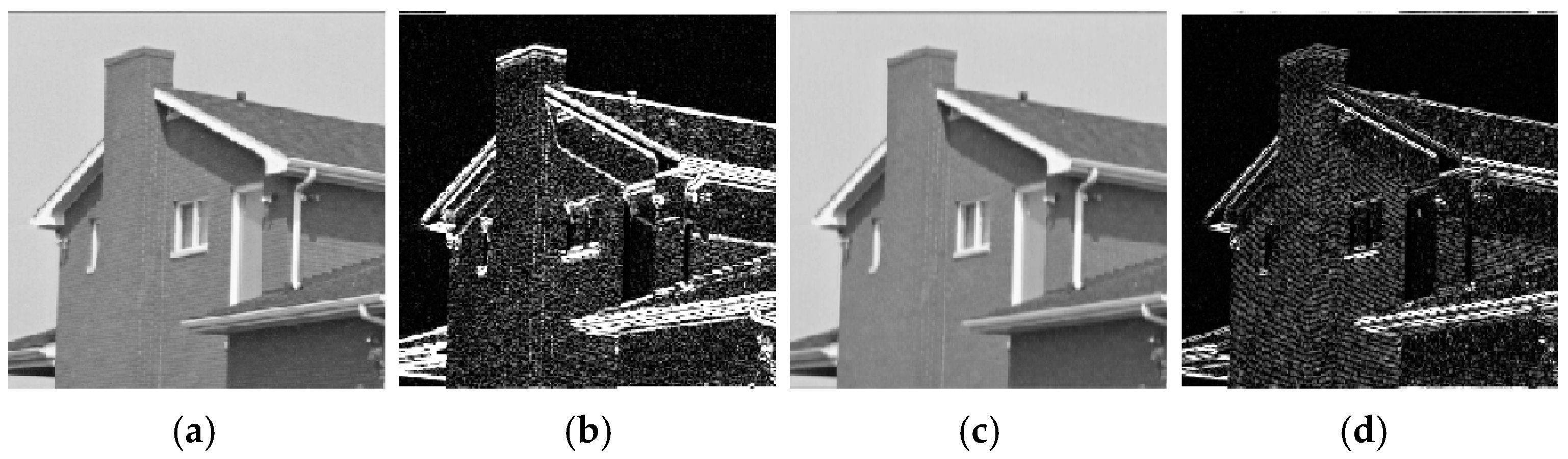
• State Preparation: The classical pixel window is normalized and embedded into a quantum state through state preparation.
• Quantum Paired Transform: The three-qubit circuit QPT is applied to the encoded state.
• Measurement and Simulation: The circuit is simulated 100,000 times using Qiskit Framework’s Aer simulator, and output probabilities are used to reconstruct amplitude-based masks.
• Mask Extraction and Visualization: Specific amplitude components (selected from indices corresponding to computational basis states) are mapped back to the [0, 255] grayscale range and stored as individual masks for the corresponding pixel of the window.

The resultant images using this process are shown below. Similar to Figure 13, Figure 17 illustrates the images composed by $c_0$(n), $c_4$(n), $c_6$(n), and $c_7$(n) coefficients in parts (a), (b), (c), and (d), respectively, using the Qiskit Framework.

Figure 18 illustrates the Leonardo Da Vinci painting ‘Lady with Ermine’, composed by $c_0$(n), $c_4$(n), $c_6$(n), and $c_7$(n) coefficients in parts (a), (b), (c), and (d), respectively, using the Qiskit Framework.

The comparable results for the grayscale images ‘pepper’, ‘cameraman’, and ‘house’ using the Qiskit Framework are shown in Figure 19, Figure 20 and Figure 21, respectively. The mean-square-root errors of calculations are given in

Table 2. The mean-square-root error (MSRE) for Figure 17, Figure 18, Figure 19, Figure 20 and Figure 21 with 10,000 shots using Qiskit.

Gradient Image	MSRE of Different Image Magnitudes
	Jetplane	Leonardo	Peppers	Cameraman	House
$c_0$	2.78 × 10−3	5.50 × 10−4	7.87 × 10−4	2.75 × 10−3	3.26 × 10−3
$c_4$	3.73 × 10−3	7.28 × 10−4	1.22 × 10−3	4.43 × 10−3	4.98 × 10−3
$c_6$	1.05 × 10−3	4.20 × 10−4	5.76 × 10−4	2.19 × 10−3	7.17 × 10−3
$c_7$	4.90 × 10−3	1.07 × 10−3	1.69 × 10−4	6.14 × 10−3	5.52 × 10−3

.

We note that the 1D convolution of length $2^r,$ or $r$-qubit convolution, can be sequentially separated by short convolutions [26]. Therefore, the presence of the schemes for short convolutions will make it possible to implement the calculation of the convolution of length $2^r,$ $r\ge 3$. The frequency characteristics of many linear time-invariant systems and filters are well known. The Fourier transform method is very efficient when computing convolution on a classical computer; the convolution is reduced to multiplication. However, it is this multiplication operation that is the most difficult step in quantum convolution using the QFT. To overcome this obstacle, we can use an additional qubit, perform the corresponding permutation, and prepare the quantum superposition of qubits for the inverse QFT. This method is described in [31] with quantum circuits for the low-pass and high-pass filters. In the general case of linear filters, the implementation of the QFT causes great difficulties and requires new quantum representations of signals, as shown in [36]. For short convolutions and gradients, the described paired-transform-based method of calculation is considered simpler than when implementing the QFT and its inverse. In this regard, we note that the Fourier transform can be calculated using only its kernel, which is the pair transform [24,33].

7. Conclusions

The quantum representation of convolutions is presented to calculate short-length convolutions and different gradients of grayscale images. For this, the quantum paired transform is used on the amplitudes of the quantum states of the convolution at each point. It is essential to determine such a representation of the image, which simplifies the procedure for calculating the convolution. Examples with convolutions and gradients with masks of lengths 3, 4, and 5 are described. These examples show that it is possible to build the circuits for the calculation of the quantum convolution. The presented method can be used for the calculation of other quantum short-length convolutions and gradients as well. There are only two limitations of this method. The impulse response of the filter or system must be known, and this method can only be applied to amplitude-represented quantum images. The paired transform is fast, binary, and is the kernel of the discrete Hadamard and Fourier transforms, which means that these two transforms can be decomposed by the sparse paired transforms. Can these transforms be used instead of the discrete paired transform in the proposed method of convolution? We hypothesize the answer is “yes” but requires further research. We strongly believe that the results presented in this article will stimulate further research in these fields. The proposed method of representation and computation can be generalized and used for other unitary transforms employed in image and signal processing, including the Hadamard transforms.

References

1. Robinson, G.S. Edge detection by compass gradient masks. Comput. Graph. Image Process. 1977, 6, 492–501. [Google Scholar]
2. Yuan, S.; Venegas-Andraca, S.E.; Wang, Y.; Luo, Y.; Mao, X. Quantum image edge detection algorithm. Int. J. Theor. Phys. 2019, 58, 2823–2833. [Google Scholar]
3. Fan, P.; Zhou, R.G.; Hu, W.; Jing, N. Quantum circuit realization of morphological gradient for quantum grayscale image. Int. J. Theor. Phys. 2019, 58, 415–435. [Google Scholar]
4. Robinson, G.S. Color edge detection. In Proceedings of the SPIE Symposium on Advances in Image Transmission Techniques, San Diego, CA, USA, 24–25 August 1976; Volume 87, pp. 126–133. [Google Scholar]
5. Pratt, W.K. Digital Image Processing, 3rd ed.; John Wiley & Sons, Inc.: Hoboken, NJ, USA, 2001. [Google Scholar]
6. Gonzalez, R.; Woods, R. Digital Image Processing, 2nd ed.; Prentice-Hall: Upper Saddle River, NJ, USA, 2002. [Google Scholar]
7. Ulyanov, S.; Petrov, S. Quantum face recognition and quantum visual cryptography: Models and algorithms. Electron. J. Syst. Anal. Sci. Educ. 2012, 1, 17. [Google Scholar]
8. Khan, M.Z.; Harous, S.; Hassan, S.U.; Khan, M.U.; Iqbal, R.; Mumtaz, S. Deep unified model for face recognition based on convolution neural network and edge computing. IEEE Access 2019, 7, 72622–72633. [Google Scholar]
9. Tan, R.C.; Liu, X.; Tan, R.G.; Li, J.; Xiao, H.; Xu, J.J.; Yang, J.H.; Zhou, Y.; Fu, D.L.; Yin, F.; et al. Cryptosystem for grid data based on quantum convolutional neural networks and quantum chaotic map. Int. J. Theor. Phys. 2021, 60, 1090–1102. [Google Scholar]
10. Cheng, C.; Parhi, K.K. Fast 2D convolution algorithms for convolutional neural networks. IEEE Trans. Circuits Syst. I Regul. Pap. 2020, 67, 1678–1691. [Google Scholar]
11. Schuld, M.; Sinayskiy, I.; Petruccione, F. An introduction to quantum machine learning. arXiv 2014, arXiv:1408.7005. [Google Scholar]
12. Kerenidis, I.; Landman, J.; Prakash, A. Quantum algorithms for deep convolutional neural network. arXiv 2019, arXiv:1911.01117. [Google Scholar]
13. Nielsen, M.; Chuang, I. Quantum Computation and Quantum Information, 2nd ed.; Cambridge University Press: Cambridge, UK, 2001. [Google Scholar]
14. Emms, D.; Wilson, R.C.; Hancock, E.R. Graph matching using the interference of discrete-time quantum walks. Image Vis. Comput. 2009, 27, 934–949. [Google Scholar]
15. Dieks, D. Communication by EPR devices. Phys. Lett. A 1982, 92, 271–272. [Google Scholar]
16. Schuld, M.; Sinayskiy, I.; Petruccione, F. The quest for a quantum neural network. Quantum Inf. Process. 2014, 13, 2567–2586. [Google Scholar]
17. Cooley, J.W.; Tukey, J.W. An algorithm the machine computation of complex Fourier series. Math. Comput. 1965, 9, 297–301. [Google Scholar]
18. Amerbaev, V.M.; Solovyev, R.A.; Stempkovskiy, A.L.; Telpukhov, D.V. Efficient calculation of cyclic convolution by means of fast Fourier transform in a finite field. In Proceedings of the IEEE East-West Design & Test Symposium (EWDTS 2014), Kiev, Ukraine, 26–29 September 2014; pp. 1–4. [Google Scholar]
19. Paul, B.S.; Glittas, A.X.; Sellathurai, M.; Lakshminarayanan, G. Reconfigurable 2, 3 and 5-point DFT processing element for SDF FFT architecture using fast cyclic convolution algorithm. Electron. Lett. 2020, 56, 592–594. [Google Scholar]
20. Blahut, R.E. Fast Algorithms for Digital Signal Processing; Addison-Wesley: Reading, UK, 1985. [Google Scholar]
21. Cleve, R.; Watrous, J. Fast parallel circuits for the quantum Fourier transform. In Proceedings of the 41st Annual Symposium on Foundations of Computer Science, Redondo Beach, CA, USA, 12–14 November 2000; pp. 526–536. [Google Scholar]
22. Yoran, N.; Short, A. Efficient classical simulation of the approximate quantum Fourier transform. Phys. Rev. A 2007, 76, 042321. [Google Scholar]
23. Perez, L.R.; Garcia-Escartin, J.C. Quantum arithmetic with the quantum Fourier transform. Quantum Inf. Process 2017, 16, 14. [Google Scholar]
24. Grigoryan, A.M.; Agaian, S.S. Paired quantum Fourier transform with log2N Hadamard gates. Quantum Inf. Process. 2019, 18, 26. [Google Scholar]
25. Caraiman, S.; Manta, V.I. Quantum image filtering in the frequency domain. Adv. Electr. Comput. Eng. 2013, 13, 77–84. [Google Scholar]
26. Grigoryan, A.M. Resolution map in quantum computing: Signal representation by periodic patterns. Quantum Inf. Process. 2020, 19, 21. [Google Scholar]
27. Argyriou, V.; Vlachos, T.; Piroddi, R. Gradient-adaptive normalized convolution. IEEE Signal Process. Lett. 2008, 15, 489–492. [Google Scholar]
28. Lomont, C. Quantum convolution and quantum correlation are physically impossible. arXiv 2003, arXiv:quant-ph/0309070. [Google Scholar]
29. Yan, F.; Iliyasu, A.M.; Venegas-Andraca, S.E. A survey of quantum image representations. Quantum Inf. Process. 2016, 15, 1–35. [Google Scholar]
30. Yan, F.; Iliyasu, A.M.; Jiang, Z. Quantum computation-based image representation, processing operations and their applications. Entropy 2014, 16, 5290–5338. [Google Scholar] [CrossRef]
31. Grigoryan, A.M.; Agaian, S.S. Quantum Image Processing in Practice: A Mathematical Toolbox, 1st ed.; Wiley: Hoboken, NJ, USA, 2025; 320p. [Google Scholar]
32. Wootters, W.K.; Zurek, W.H. A single quantum cannot be cloned. Nature 1982, 299, 802–803. [Google Scholar]
33. Grigoryan, A.M.; Grigoryan, M.M. Brief Notes in Advanced DSP: Fourier Analysis with MATLAB; CRC Press Taylor and Francis Group: Boca Raton, FL, USA, 2009. [Google Scholar]
34. Qiskit Development Team. Qiskit: An Open-Source Framework for Quantum Computing, Version 1.3.2. Computer software. IBM Quantum: Poughkeepsie, NY, USA, 2019.
35. Yao, X.W.; Wang, H.; Liao, Z.; Chen, M.C.; Pan, J.; Li, J.; Zhang, K.; Lin, X.; Wang, Z.; Luo, Z.; et al. Quantum image processing and its application to edge detection: Theory and experiment. Phys. Rev. X 2017, 7, 031041. [Google Scholar]
36. Grigoryan, A.M.; Agaian, S.S. 3-Qubit circular quantum convolution computation using the Fourier transform with illustrative examples. J. Quantum Comput. 2024, 6, 1–14. [Google Scholar]
Figure 1. Image gradient computation by a quantum computer.
Information 16 00255 g001
Figure 2. The f o u r -point strong DsiHT on the generator.
Information 16 00255 g002
Figure 3. The quantum scheme of the two-qubit QsiHT with the generator ( 1,2 , 2,1 ) .
Information 16 00255 g003
Figure 4. The quantum scheme of the two-qubit-to-two-qubit transform q y .
Information 16 00255 g004
Figure 5. The quantum circuit for the two-qubit QPT.
Information 16 00255 g005
Figure 6. The circuit element for processing the two-qubit y n .
Information 16 00255 g006
Figure 7. (a) The grayscale image ‘house.tiff’ and (b) the c 0 -gradient image (in the absolute scale), (c) the c 2 -smooth image, and (d) c 3 -gradient image.
Information 16 00255 g007
Figure 8. (a) The original grayscale image, (b) the c 0 -gradient image, (c) c 2 -smooth image, and (d) c 3 -gradient image.
Information 16 00255 g008
Figure 9. The quantum circuit for the two-qubit QPT of the superposition | χ 4 ( y n ) .
Information 16 00255 g009
Figure 10. (a) The model of the measurement transforms and (b) the simulated measured ‘jetplane’ image with c 0 , c 2 , and c 3 -coefficients.
Information 16 00255 g010
Figure 12. The circuit element for processing the superposition y n .
Information 16 00255 g012
Figure 13. (a) The c 0 -gradient image, (b) the c 4 -gradient image, (c) c 6 -smooth image, and (d) c 7 -gradient image.
Information 16 00255 g013
Figure 14. (a) The model of the measurements that transforms and (b) the simulated measured ‘jetplane’ image with c 0 ,   c 2 ,   c 4 ,   c 6 , and c 7 -coefficients.
Information 16 00255 g014
Figure 15. (a) The grayscale image [leonardo9.jpg] of size 744 × 526 pixels (from http://www.abcgallery.com, accessed on 9 September 2017) and (b) the computer-simulated measured image with c 0 , c 2 ,   c 4 , c 6 , and c 7 -amplitudes.
Information 16 00255 g015
Figure 16. (a) The grayscale ‘pepper’ and (b) the simulated random image with c 0 , c 2 , c 4 , c 6 , and c 7 -amplitudes.
Information 16 00255 g016
Figure 17. (a) The c 0 -gradient image, (b) the c 4 -gradient image, (c) c 6 -smooth image, and (d) c 7 -gradient image of ‘jetplane’ using the Qiskit Framework.
Information 16 00255 g017
Figure 18. (a) The c 0 -gradient image, (b) the c 4 -gradient image, (c) c 6 -smooth image, and (d) c 7 -gradient image using the Qiskit Framework.
Information 16 00255 g018
Figure 19. (a) The c 0 -gradient image, (b) the c 4 -gradient image, (c) c 6 -smooth image, and (d) c 7 -gradient image using the Qiskit Framework.
Information 16 00255 g019
Figure 20. The cameraman image with (a) c 0 -gradient image, (b) the c 4 -gradient image, (c) c 6 -smooth image, and (d) c 7 -gradient image using the Qiskit Framework.
Information 16 00255 g020
Figure 21. The “house” image with (a) c 0 -gradient image, (b) the c 4 -gradient image, (c) c 6 -smooth image, and (d) c 7 -gradient image using the Qiskit Framework.
Information 16 00255 g021