Abstract
Alzheimer’s disease (AD) is a persistent neurologic disorder that has no cure. For a successful treatment to be implemented, it is essential to diagnose AD at an early stage, which may occur up to eight years before dementia manifests. In this regard, a new predictive machine learning model is proposed that works in two stages and takes advantage of both unsupervised and supervised learning approaches to provide a fast, affordable, yet accurate solution. The first stage involved fuzzy partitioning of a gold-standard dataset, DARWIN (Diagnosis AlzheimeR WIth haNdwriting). This dataset consists of clinical features and is designed to detect Alzheimer’s disease through handwriting analysis. To determine the optimal number of clusters, four Clustering Validity Indices (CVIs) were averaged, which we refer to as cognitive features. During the second stage, a predictive model was constructed exclusively from these cognitive features. In comparison to models relying on datasets featuring clinical attributes, models incorporating cognitive features showed substantial performance enhancements, ranging from 12% to 26%. Our proposed model surpassed all current state-of-the-art models, achieving a mean accuracy of 99%, mean sensitivity of 98%, mean specificity of 100%, mean precision of 100%, and mean MCC and Cohen’s Kappa of 98%, along with a mean AUC-ROC score of 99%. Hence, integrating the output of unsupervised learning into supervised machine learning models significantly improved their performance. In the process of crafting early interventions for individuals with a heightened risk of disease onset, our prognostic framework can aid in both the recruitment and advancement of clinical trials.
1. Introduction
Dementia poses a formidable global health challenge, impacting over 55 million individuals worldwide, with pronounced effects on low- and middle-income nations []. Annually, close to 10 million new cases emerge, positioning it as the seventh leading cause of mortality and placing a significant strain on global healthcare systems []. Among the elderly, dementia is a primary contributor to disability and dependence, with informal caregivers devoting an average of 5 h per day to care-giving duties [,]. Notably, women shoulder a disproportionate share, accounting for 70% of care-giving hours. Alzheimer’s disease (AD) represents the majority of dementia cases, ranging from 60% to 70% [], and is characterized by progressive cognitive decline and extensive neural damage and atrophy in muscle tissue [,]. With the absence of curative interventions, early diagnosis remains pivotal before dementia symptom onset [,]. With global life expectancy on the rise, the incidence of neurodegenerative disorders is projected to surge in the forthcoming decades []. Estimates suggest that by 2050, the number of individuals affected by AD and other dementia will soar to 152 million [] or even more [,], underscoring the urgent need for advanced clinical approaches to bolster early detection.
The progression of Alzheimer’s disease (AD) can be more accurately described using the 7-stage model [], as outlined in Table 1. Early diagnosis of AD holds significant potential [], particularly when patients remain functionally independent (Stage 2 or 3 of the 7-stage model) and are dementia-free []. This early detection window may extend up to 8 years before the onset of dementia symptoms []. In the pursuit of early Alzheimer’s detection, we introduce a novel hybrid machine learning (ML) model that blends unsupervised cognition and supervised learning. This model utilizes a gold-standard dataset called DARWIN (Diagnosis AlzheimeR WIth haNdwriting), comprising 1D features extracted from handwriting analysis following the protocol outlined in Cilia et al.’s work []. Leveraging handwriting analysis for detecting Alzheimer’s disease has its own advantages, as it is a non-invasive and cost-effective approach. Further, it can function as a pre-screening procedure, before resorting to more costly medical diagnoses such as MRI or PET scans.

Table 1.
Stages and levels of cognitive impairment. This table outlines the various stages of cognitive impairment, along with their corresponding levels of decline.
Employing two distinct methodologies, unsupervised and supervised learning within a unified model, we characterize our model as a hybrid model operating in two stages. The model first employs a fuzzy-logic-based unsupervised learning algorithm on the DARWIN dataset to generate a fuzzy membership matrix corresponding to the optimal number of cluster centers, crucial for understanding patient condition patterns. Fuzzy logic is predominantly utilized in this study due to its ability to effectively address uncertainties inherent in data, particularly in fields such as medical diagnosis, where precision in diagnosis may be crucially enhanced via fuzzification [].
We conceptualize the fuzzy membership matrix as a dataset imbued with cognitive features. In this analogy, each cluster center represents a distinct cognitive feature, while the membership degree of a handwriting sample corresponds to the value of that feature. The term “cognitive feature” is employed to signify the output of the Fuzzy C-Means algorithm, as it encapsulates patterns extracted from handwriting data believed to correlate with cognitive function, particularly in the context of Alzheimer’s disease prediction. In the second stage, these cognitive features serve as inputs for constructing predictor models using supervised learning techniques. We anticipate that employing unsupervised cognitive values will enhance the performance of supervised ML models, promising more accurate Alzheimer’s risk identification and dementia prevention. The main contributions of this study can be summarized as follows:
- Introduction of a Novel Hybrid Model: The research introduces a novel predictive model designed to identify Alzheimer’s disease (AD) at an early stage (in stage 2 or 3, as mentioned in Table 1). This hybrid model seamlessly integrates both unsupervised and supervised approaches, delivering a harmonious blend of rapidity, streamlined design, and enhanced accuracy that surpasses current state-of-the-art methodologies.
- Integration of Fuzzy Logic with Machine Learning: A creative strategy merges “Fuzzy Logic” with “Machine Learning”, enhancing the efficacy of conventional classifiers and introducing a novel dimension into medical diagnosis.
- Lightweight Model for Medium Datasets: Introducing a lightweight model tailored for training on medium-sized datasets, ensuring practicality and efficiency, especially in settings with limited data accessibility.
- Comprehensive Set of Baselines: Incorporating a diverse set of baseline classifiers for benchmarking, enabling a thorough assessment of the proposed model against existing methods of AD detection.
- Use of Clustering Validity Index: Multiple clustering validity indices are employed to determine the optimal number of clusters, enhancing data pattern comprehension by considering membership values.
- Extensive Hyperparameter Optimization: Automated hyperparameter optimization ensures the identification of the most optimal model, resulting in enhanced accuracy in AD detection.
Related Work
Machine learning (ML) has become a powerful tool for predicting neurodegenerative diseases [,,,,,,], including Alzheimer’s disease (AD), through the analysis of various data types, including medical images [,,,,,], genetic information [,,], cognitive assessments [,,], and multi modal approaches []. However, the utilization of handwriting-based analysis holds its own significance. This form of cognitive assessment offers a direct measure of brain function, capturing individual motor patterns [,] and is a well-established means for detection of neurodegenerative diseases [,,,,,]. Furthermore, due to its non-invasive nature and cost-effectiveness, such a technique could be considered a pre-screening routine by practitioners, before resorting to expensive diagnostic methods such as MRI and PET scans. This makes it particularly appealing in low- and middle-income countries, which account for 60% of global Alzheimer’s disease incidents []. Despite being a significant cause of dementia, attempts to predict AD through handwriting analysis remain limited, due to the lack of benchmark datasets.
Crafting a benchmark dataset hinges on establishing a meticulously defined protocol for both data collection and subsequent analysis. Recognizing the significance of a standardized protocol in constructing such a benchmark dataset, Cilia et al. [] introduced a comprehensive protocol for collecting and analyzing handwriting data to detect Alzheimer’s disease. Their protocol recommends the use of 25 specific tasks (detailed descriptions of the tasks are given in Supplementary Table S1), designed based on insights from motor control and neuroscience. Each task aims to delve into the intricate dynamics of how specific brain regions contribute to both handwriting and drawing movements performed by the participants. By elucidating how deviations in these brain regions manifest in the overall progression of Alzheimer’s disease, the protocol further describes each task using 18 unique measurable features (detailed descriptions of the features are given in Supplementary Table S2). This collaborative effort culminated in the creation of the DARWIN dataset (Diagnosis AlzheimeR WIth haNdwriting) with 450 features (25 tasks × 18 features per task), representing the largest publicly available, as well as comprehensive and invaluable, resource for applying machine learning techniques to analyze handwriting data in the context of Alzheimer’s disease diagnosis.
Building upon previous research conducted in [,], the present investigation acknowledges an opportunity to refine the existing predictive model for Alzheimer’s disease (AD) by leveraging handwriting analysis with the DARWIN dataset. In the study by De Gregorio [], a set of classifiers, particularly Random Forest (RF), K-Nearest-Neighbor (KNN), Linear Discriminant Analysis (LDA), Gaussian Naive Base (GNB), and Support Vector Machine (SVM) models, were trained using task-specific features, resulting in multiple predictors of AD based on particular tasks. Subsequently, these predictors were amalgamated to form the final prediction model. The development of task-specific predictors entailed the application of a single type of machine learning algorithm. Their findings suggest that, when employing Random Forest (RF) to construct task-specific classifiers and then ensemble them, the achieved performance metrics were notable: an overall accuracy of 91%, with a sensitivity of 83% and a specificity of 100%.
In contrast, Cilia et al. [] employed diverse machine learning algorithms (Random Forest, Logistic Regression, K-Nearest Neighbor, Linear Discriminant Analysis, Gaussian Naive Bayes, Support Vector Machine, Decision Tree, Multilayer Perceptron, and Learning Vector Quantization) to construct task-specific models, combining the best-performing models for the ultimate prediction by ensembling them. They achieved a highest accuracy of 94.28%, specificity of 88.24%, and sensitivity of 100%. However, both approaches treated the set of task-specific features as a unified entity, overlooking potential correlations among the features.
In a notable study by Parziale et al. [], an intriguing approach was taken to evaluate the performance of three one-class classifier models—namely, the Negative Selection Algorithm, the Isolation Forest, and the One-Class Support Vector Machine—on the DARWIN dataset. Remarkably, they achieved an accuracy of 97.12%, a sensitivity of 94.23%, and a specificity of 100.00% with the random Negative Selection Algorithm.
In the study of Subha R. et al. [], a hybrid ML model with Swarm Intelligence (SI)-based feature selection was developed for detection of Alzheimer’s disease. They employed several machine learning models, specifically LR, KNN, SVM, DT, RF, and AdaBoost, achieving a highest accuracy of 90%, precision of 88%, recall of 92%, F1-score 90%, and AUC-ROC score 90% with the RF and AdaBoost classifiers.
In Gattulli V. et al. [], a wide set of classification models, including Random Forest (RF), Logistic Regression (LR), K-Nearest Neighbor (KNN), Linear Discriminant Analysis (LDA), Support Vector Machines (SVM), Bayesian Networks (BN), Gaussian Naïve Bayes (GNB), Multilayer Perceptron (MP), and Learning Vector Quantization (LVQ), were used for a group of selected tasks, encompassing different types of writing and drawing tasks, and varying levels of complexity, from simple to more complex tasks. Their reported highest accuracy was 88%, with a specificity of 86% and sensitivity of 90% with RF classifiers.
In the work of Onder M. et al. [], the authors conducted a comprehensive study to diagnose AD using four different categorization methods. These methods included XGBoost, GradientBoost, AdaBoost, and Voting Classification algorithms. The highest accuracy obtained was 85% by the XGBoost classifier.
In Hakan Ö et al. [], a tipple ensemble machine learning model was developed and applied for AD detection, using Light Gradient Boosting Machine, Categorical Boosting, and Adaptive Boosting machine learning classification algorithms combined with a Hard Voting Classifier. The reported results of the experimental studies using the proposed ensemble methodology were 97.14% Acc, 95% Prec, 100% Recall, 90.25% Spec, and 97.44% F1-score.
In Mitra and Rehman [], a stacking-based ensemble integrating multiple classifiers achieved superior performance metrics, including 97.14% accuracy, 95% sensitivity, and 100% specificity. Feature selection methods like ANOVA and RFE further enhanced the model performance.
Interestingly, along with machine-learning-based approaches, deep-learning-based models have also been applied on the DARWIN dataset for detection of AD. On the other hand, in Erdogmus P. et al. [], a Convolutional Neural Network (CNN) was employed on the DARWIN dataset designed for AD detection through handwriting. They extracted 2D features from the original 1D dataset and applied these to their proposed model. Training and evaluation on this 2D dataset resulted in a 90.4% accuracy for their proposed model. This suggests the potential of deep learning approaches for early and effective AD diagnosis.
In conclusion, while current methods for Alzheimer’s Disease (AD) detection show promise, there is a clear need for methodological advancement. Despite achieving commendable accuracies, future research should focus on refining feature selection, exploring new algorithmic approaches, and incorporating additional data sources. By continually improving upon existing methodologies, the field of AD detection can advance towards earlier and more effective diagnosis. Table 2 presents a summary of the recent methods targeting the DARWIN dataset, while in Figure 1, we present a workflow of the proposed approach and Table 2 presents it in detail.
Table 2.
Workflow stages and their purpose.
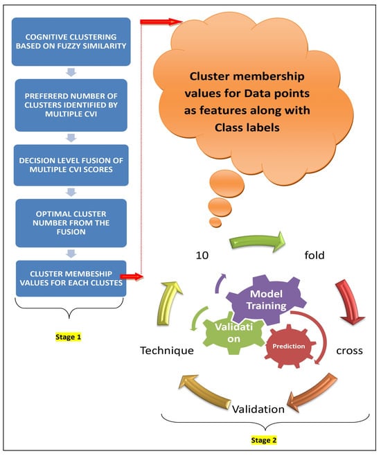
Figure 1.
The workflow of the proposed approach.
2. Materials and Methods
In this section, we present a description of the (i) dataset construction, (ii) software stack used for end-to-end implementation of the model, (iii) development of the proposed novel model, (iv) performance evaluation metrics, and (v) training of the proposed model.
2.1. Dataset Construction
The DARWIN (Diagnosis AlzheimeR WIth haNdwriting) dataset has been meticulously curated to facilitate the early detection of Alzheimer’s disease by analyzing handwriting features based on clinical processes. This valuable dataset is openly accessible at https://archive.ics.uci.edu/dataset/732/darwin (accessed on 15 March 2025), containing data from 174 individuals. Among them, 89 persons were diagnosed with Alzheimer’s disease, while 85 were healthy participants. The demographic information about the dataset is presented in Table 3. The dataset was created by combining data from 25 unique neuroscience guide tasks, categorized as Memory and dictation (M), Graphic (G), and Copy (C), as described in Supplementary Table S1. Each task contributes 18 distinct handwriting features, detailed in Supplementary Table S2. In total, this compilation comprises 450 features (25 tasks × 18 features per task), providing a comprehensive resource for researchers and professionals involved in the early diagnosis of Alzheimer’s disease. The term clinical feature is henceforth used to denote these 450 features.
Table 3.
Summary of studies on Alzheimer’s disease prediction using the DARWIN dataset.
2.1.1. Handwriting Data Collection Process
To assess handwriting characteristics in individuals with Alzheimer’s Disease (AD), a structured set of 25 handwriting tasks was used. These tasks were carefully designed to evaluate different aspects of motor function (M), cognitive abilities (C), and graphical skills (G), which are often affected in AD.
Participants were given specific instructions to perform tasks such as drawing shapes, copying letters or words, writing dictated sentences, and recalling written information (details of these tasks are described in Supplementary Table S1). These tasks were performed using a digital tablet and stylus, which captured detailed handwriting movements in real time. The device recorded stroke patterns, speed, pressure, and tremor-related variations that are not visible to the naked eye. The collected handwriting data serve as a potential indicator of neurological and cognitive decline in AD patients.
Healthcare professionals supervised the process to ensure participants followed the instructions correctly, minimizing external influences like fatigue or stress that could have affected the results. The data were then stored digitally for further analysis.
2.1.2. Feature Extraction from Handwriting Data
After collecting handwriting samples, various features (details of these features are described in Supplementary Table S2) were extracted to quantify writing performance and detect abnormalities associated with AD. These features fall into different categories:
2.1.3. Time-Based Features (How Long the Writing Takes)
- Total Time (TT): Measures the total duration required to complete a task.
- Air Time (AT) & Paper Time (PT): Differentiates between the time spent writing on the paper and the time when the pen is lifted. A longer air time may indicate hesitation or difficulty in initiating movement.
2.1.4. Speed and Movement Features (How the Hand Moves During Writing)
- Mean Speed on-paper (MSP) & Mean Speed in-air (MSA): Measure the average speed of writing and movement in the air, which may be slower in AD patients due to motor impairments.
- Mean Acceleration (MAP, MAA): Assesses how quickly writing speed changes, indicating the ability to control movement.
- Mean Jerk (MJP, MJA): Measures how smoothly or abruptly the hand moves, providing insights into motor control and stability.
2.1.5. Pressure-Based Features (How Hard the Pen Is Pressed on the Paper)
- Pressure Mean (PM) & Pressure Variance (PV): Assess the force applied while writing. Inconsistencies in pressure may suggest declining motor function or hand tremors.
2.1.6. Tremor and Stability Features (How Steady the Writing Is)
- Generalized Mean Relative Tremor (GMRT, GMRTP, GMRTA): Identifies hand tremors, which are common in neurological disorders.
2.1.7. Spatial and Structural Features (How Writing Is Organized on the Page)
- Max X and Y Extensions (XE, YE): Measures the size of handwriting strokes. Changes in stroke size can indicate cognitive and motor decline.
- Dispersion Index (DI): Evaluates whether handwriting is spread evenly or scattered, which may reflect spatial planning difficulties.
2.1.8. Task-Specific Features (Additional Behavioral Indicators)
- Pen-down Number (PWN): Counts how many times the pen touches the paper, reflecting writing fluency and control.
Once these features had been extracted, they were analyzed using statistical and machine learning techniques to identify patterns that differentiated AD patients from healthy individuals. This approach provides objective, quantifiable measures that can complement traditional clinical assessments for early detection of Alzheimer’s disease.
2.2. Software Stack
The software stack employed for system development encompassed a collection of Python libraries optimized for various stages of machine learning development, from data preprocessing to model evaluation. These libraries included
- pandas and numpy: These libraries are fundamental for data manipulation, providing efficient data structures and array operations necessary for handling and processing datasets.
- sklearn.preprocessing.StandardScaler: Used for standardizing data, ensuring features are on the same scale, which is crucial for many machine learning algorithms to perform optimally.
- scikit-learn (sklearn): This library forms the backbone of the machine learning pipeline, offering a comprehensive suite of algorithms and tools for modeling, evaluation, and cross-validation. Specific classifiers utilized included
- DecisionTreeClassifier (DT)
- RandomForestClassifier (RF)
- ExtraTreesClassifier (ET)
- LogisticRegression (LR)
- LinearDiscriminantAnalysis (LDA)
- GaussianNB (GNB)
- XGBClassifier (XGB)
- DecisionTreeClassifier (DT)
- MLPClassifier (MLP)
- KNeighborsClassifier (KNN)
- matplotlib: Employed for data visualization, enabling the generation of insightful plots and graphs for data exploration, model evaluation, and comparison of results across different algorithms.
This software stack provides a robust environment for developing and analyzing machine learning models, covering a diverse range of algorithms and techniques suitable for various types of datasets and problem domains.
2.3. Development of the Proposed Model
The hybrid prognostic model presented in this study was formulated through a two-stage approach. A data-centric schematic representation of the model development process is illustrated in Figure 2.
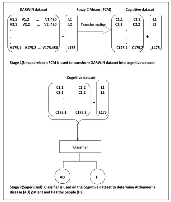
Figure 2.
The data-centric model development process consisted of two stages. In Stage 1, unsupervised machine learning was employed, while Stage 2 involved the application of supervised machine learning. Within the context of the DARWIN dataset, Vi,j represents the jth feature value of the ith handwriting sample. Ci,j denotes the fuzzy membership value corresponding to the jth cluster center for the ith handwriting sample, while Li indicates the class label for the ith handwriting sample. It is important to note that in Stage 1, only the values Vi,j were input into the FCM algorithm. The labels were explicitly appended to the output of the FCM (Fuzzy C-Means) algorithm to train the supervised learning algorithms.
2.3.1. Stage 1: Cognitive Feature Generation Using Unsupervised Learning
In the initial phase, we employed the Fuzzy C-Means (FCM) algorithm to facilitate grouping of the handwriting samples in the DARWIN dataset based on clinical features. Let, be the set of handwriting samples, where each and in our case. The objective function of the Fuzzy C-means algorithm is given by
where
- is the fuzzy membership matrix, with representing the membership of data point to cluster j.
- is the matrix of cluster centers, with .
- is the fuzzifier parameter, controlling the degree of fuzziness.
Being an iterative algorithm, the steps involved in the Fuzzy C-means algorithm can be described as as follows:
- Initialize U and V.
- Repeat until convergence:
- (a)
- Update cluster centers :
- (b)
- Update the fuzzy membership matrix U:
We conceptualized the fuzzy membership matrix U as a dataset imbued with cognitive features. In this analogy, each cluster center represents a distinct cognitive feature, while the membership value of a handwriting sample corresponds to the value of that feature. Consequently, this perspective enabled us to interpret the transformation of 450 clinical features into cognitive features, leveraging the proficiency of FCM in handling the uncertainty inherent in medical data.
An important consideration when utilizing FCM is the determination of the optimal number of cluster centers, as this directly influences the data partitioning process. By selecting an appropriate number of cluster centers, we could effectively uncover significant patterns within the data and accurately perform a categorization. To quantitatively assess cluster quality and separation, we employed four widely recognized Clustering Validity Indices (CVIs): Silhouette Score [], Davies–Bouldin Score [], Calinski–Harabasz Score [], and Dunn Score []. Clustering Validity Indices (CVIs) serve as metrics for evaluating the quality of clustering outcomes derived from clustering algorithms. Below, we elaborate on these four commonly utilized CVIs:
Silhouette Score: The Silhouette Score is a measure of how similar an object is to its own cluster (cohesion) compared to other clusters (separation). It is calculated for each data point i using the following formula:
where
- is the average distance from point i to other points within the same cluster.
- is the smallest average distance from point i to points in a different cluster.
The Silhouette Score for the entire dataset is the average of the Silhouette scores of all data points.
Davies–Bouldin Score: The Davies–Bouldin Score evaluates the average similarity between each cluster and its most similar cluster, relative to the average dissimilarity between points in different clusters. It is calculated as
where
- k is the number of clusters.
- and are clusters.
- is a measure of similarity between clusters and .
- is a measure of dissimilarity between clusters and .
A lower Davies–Bouldin Score indicates better clustering.
Calinski–Harabasz Score: The Calinski–Harabasz Score, also known as the Variance Ratio Criterion, measures the ratio of between-cluster dispersion to within-cluster dispersion. It is given by
where
- B is the between-cluster dispersion.
- W is the within-cluster dispersion.
- N is the total number of data points.
- k is the number of clusters.
A higher Calinski–Harabasz Score indicates denser and better-separated clusters.
Dunn Score: The Dunn Score assesses the compactness and separation of clusters. It is calculated as
where
- is the separation between clusters and .
- is the diameter of cluster .
A higher Dunn Score indicates better clustering, with compact and well-separated clusters.
2.3.2. Stage 2: Prognostic Model Development Using Supervised Learning
In the second stage, we utilized a fuzzy membership matrix U, hereafter referred to as the cognitive dataset, to develop a predictor for Alzheimer’s disease (AD) cases. Supervised machine learning involves leveraging a labeled training dataset to construct models capable of discerning patterns within data. These well-trained models are subsequently applied to an unlabeled testing dataset to accurately categorize its contents. During the training phase of our proposed supervised learning model, we employed the ground truths provided by the DARWIN dataset as labels for the cognitive dataset generated in stage 1. In this section, we present a succinct overview of ten state-of-the-art supervised machine learning algorithms [] that have been employed to build models for the early detection of Alzheimer’s disease.
Decision Tree (DT): A Decision Tree recursively splits data based on the most significant attribute. There is no specific mathematical equation for a Decision Tree itself, but it uses criteria like Gini impurity or entropy for splitting.
Random Forest (RF): Random Forest is an ensemble of decision trees. The final prediction is obtained by averaging or taking a majority vote from the individual trees.
Extra Trees (Extra Tree): Extra Trees, like Random Forest, is an ensemble of decision trees but with more randomness in feature selection and splitting. It uses the same mathematical rules for splitting nodes as traditional decision trees.
Logistic Regression (LR): Logistic Regression models the probability of an instance belonging to a particular class using the logistic function (sigmoid function).
Linear Discriminant Analysis (LDA): LDA finds the linear combinations of features that maximize the separation between different classes. Mathematical Equation for Linear Discriminant Analysis:
where is the weight vector and is the linear discriminant.
Gaussian Naive Bayes (GNB): GNB is based on Bayes’ theorem and assumes that features are conditionally independent given the class. Mathematical Equation for Naive Bayes:
XGBoost (XGB): XGBoost is a gradient boosting algorithm that minimizes a loss function by adding decision trees iteratively. Objective Function in XGBoost:
k-Nearest Neighbors (KNNs): KNNs assigns a class label to an instance based on the majority class among its k nearest neighbors. There is no specific mathematical equation for KNNs, but it uses distance metrics like Euclidean or Manhattan distance.
Support Vector Machine (SVM): A SVM finds the hyperplane that best separates different classes with the maximum margin. Mathematical Equation for Linear SVM:
Multi-Layer Perceptron (MLP): A MLP is a type of artificial neural network with multiple layers of interconnected nodes, including input, hidden, and output layers. Mathematical Equations for Forward Propagation:
The weights in MLPs are learned through an iterative optimization process using backpropagation, where the network minimizes the error by adjusting weights based on the gradient of a loss function with respect to these weights. This is typically achieved via gradient descent or its variants. While a full discussion of backpropagation is beyond the scope of this article, it plays a crucial role in training MLPs by propagating errors backward and updating the weights accordingly.
2.3.3. The Proposed Model with Optimal Setup
The proposed model stands out for its algorithms and their respective hyperparameters. In Stage 1, we iteratively applied the Fuzzy C-Means (FCM) algorithm to the DARWIN dataset to ascertain the optimal number of cluster centers, denoted as k, a pivotal hyperparameter in the model. We determined the preferred number of cluster centers to be 2, using an average scoring scheme derived from the amalgamation of four normalized CVI scores.
In Stage 2, we employed ten supervised learning algorithms, alongside the FCM algorithm, to identify the most effective classifier. A crucial step involved fine-tuning the hyperparameters, achieved through the widely adopted Grid-Search-CV method. Grid Search Cross-Validation (Grid Search CV) systematically explores a predefined grid of hyperparameters, assessing each combination’s performance through cross-validation, typically k-fold cross-validation. The optimal configuration is selected based on the best performance metrics on the validation set. Furthermore, we utilized 10-fold cross-validation with the chosen optimal hyperparameter values for each classifier, to evaluate its performance. Notably, Random Forest (RF) emerged as the most effective approach, in conjunction with the FCM algorithm, for predicting Alzheimer’s disease. For detailed parameter configurations, please refer to Table 4.
Table 4.
Average demographic data of participants. Standard deviations are shown in parentheses.
2.4. Algorithm
The algorithmic representation of the proposed model comprises three parts: Algorithms 1–3. Stage 1 is delineated into two distinct procedures: “CogniGen”, outlined in Algorithm 1, and the Fuzzy C-Means, detailed in Algorithm 2, whereas Stage 2 is represented in Algorithm 3.
| Algorithm 1 CogniGen computes “cognitive features” from “clinical features” |
| Input: Dataset X, maximum number of clusters N, fuzziness parameter m, termination criterion , maximum number of iterations I. Output: Optimal number of clusters , Final Cluster Centers , Fuzzy Membership Matrix , Silhouette Scores array S, Davies–Bouldin Scores array , Calinski–Harabasz Scores array , Dunn Scores array D for to N.
|
| Algorithm 2 Fuzzy C-Means Clustering |
| Input: Dataset X, number of clusters C, fuzziness parameter m, termination criterion , maximum number of iterations. Output: Cluster centers , Membership matrix U.
|
| Algorithm 3 Random Forest Algorithm |
|
2.5. Performance Evaluation Metrics
To identify the most precise set of classifiers, we analyzed and compared the scores of seven widely used performance metrics in machine learning: accuracy, sensitivity, specificity, precision, Matthews Correlation Coefficient (MCC), Cohen’s Kappa, and AUC-ROC. In the subsequent section, we present a concise overview of the performance evaluation metrics employed in our study.
All the performance metrics in machine learning are based on the concept of a confusion matrix, which is a table (Table 5) used to assess the performance of a classification algorithm. The main components of a confusion matrix are
Table 5.
Proposed Model and Hyperparameters.
- True Positive (TP): The number of instances correctly predicted as positive.
- True Negative (TN): The number of instances correctly predicted as negative.
- False Positive (FP): The number of instances incorrectly predicted as positive.
- False Negative (FN): The number of instances incorrectly predicted as negative.
1. Accuracy (Acc): The ratio of correctly predicted instances to the total number of instances in the dataset.
2. Sensitivity (SN): The proportion of actual positive cases that are correctly identified by the model.
3. Specificity (SP): The proportion of actual negative cases that are correctly identified by the model.
4. Precision: The ratio of correctly predicted positive observations to the total predicted positive observations.
5. Matthews Correlation Coefficient (MCC): A measure of the quality of binary classifications, taking into account true and false positives and negatives.
6. Cohen’s Kappa: A statistic measuring inter-rater agreement for qualitative items, accounting for agreements occurring by chance.
7. Area Under the Receiver Operating Characteristic Curve (AUC ROC): A performance measurement for classification problems, representing the area under the ROC curve.
2.6. Training of the Proposed Model
As a two-stage model, Stage 1 operates unsupervised, while Stage 2 is supervised. Setting up the working environment for the model required careful consideration. In Stage 1, we began by isolating the class label component from the DARWIN dataset and feeding it into the FCM algorithm. Since FCM is an unsupervised learning method, it autonomously extracted significant patterns from the data and did not require class information. Thus, in Stage 1, we observed the transformation of the DARWIN dataset into the cognitive dataset.
Moving to Stage 2, which operated under a supervised paradigm, we had to additionally merge the class label with the cognitive dataset generated in Stage 1. This amalgamated cognitive dataset, inclusive of class labels, served as the foundation for training, cross-validation, and evaluation of the supervised learning algorithms.
The cognitive dataset was initially split into a training set (80%) and a held-out set (20%). The training set was then used for both hyperparameter tuning through GridSearchCV and subsequent model evaluation via 10-fold cross-validation. GridSearchCV optimized the model hyperparameters by internally employing cross-validation, and we used 5-fold cross validation. Following hyperparameter selection, 10-fold cross-validation assessed the model’s performance across various subsets of the training data. Finally, the model’s performance was validated on the held-out test set (20%), providing an unbiased estimate of its generalization to unseen data. This methodology effectively utilized the available data for model development and evaluation, while ensuring a robust performance estimation through separate test data evaluation. Furthermore, we repeated the whole procedure 10 times. This iterative approach enhanced the confidence in the model’s predictive capabilities and guarded against overfitting or biases introduced by a single train–test split.
3. Results
Our research efforts spanned a broad spectrum of experiments geared towards crafting a reliable and precise tool for detecting Alzheimer’s disease in its early stages. Using a two-stage approach, our experiments can be classified into those utilizing unsupervised learning techniques and others employing supervised learning methods. All experiments were carried out on a modest computational setup comprising an Intel(R) Core(TM) i5-5200U CPU @ 2.20 GHz, 4GB RAM, and a 1TB HDD, supplemented by computational resources from the freely accessible version of Google Colab.
3.1. Results from Unsupervised Machine Learning
During the initial stage of our experimentation with the DARWIN dataset, we embarked on a meticulous process. Beginning by parsing the dataset, we segregated the class labels from the feature matrix component. With this separation in place, we commenced the application of the Fuzzy C Means algorithm on the feature matrix for our clustering objectives. This algorithm efficiently processed the handwriting samples encapsulated within the feature matrix, leveraging its flexibility to accommodate a user-defined number of cluster centers, denoted as k. As a result of this process, we obtained a crucial output—the fuzzy membership matrix , intricately linked to the designated cluster center values k.
To proceed with informed decision-making in the subsequent stage, we undertook a comprehensive assessment of the clustering outcomes. Initially, we embarked on a systematic exploration, computing Cluster Validity Index (CVI) scores across a spectrum of k values, meticulously spanning a range of consecutive integers denoted by . This endeavor provided us with a nuanced understanding of the clustering performance across varying degrees of granularity in cluster representation. Figure 3 visually encapsulates the diversity of clustering outcomes, portraying the fuzzy membership matrices corresponding to distinct k values, facilitating visual comprehension of the clustering dynamics.
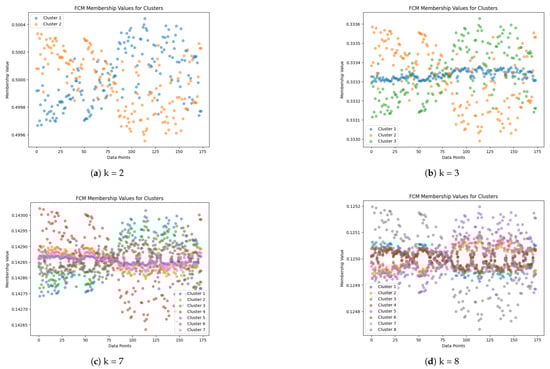
Figure 3.
Fuzzy membership matrices corresponding to cluster centers for different values of k: (a) , (b) , (c) , and (d) . The y-axis represents each of the handwriting samples, while the x-axis denotes their fuzzy membership values corresponding to each cluster center. Figures should be placed in the main text near the first time they are cited.
Determining the optimal configuration of cluster centers constituted a pivotal aspect of our analysis. Through an iterative process guided by the CVI function, we aimed to pinpoint the value of k that maximized the clustering efficacy across the entire spectrum of . This task necessitated the integration of multiple perspectives, requiring a judicious amalgamation of insights derived from a diverse set of metrics. Employing an average scoring mechanism, we distilled the complexities of the clustering performance into a succinct evaluation criterion, aggregating normalized CVI scores across the four key metrics mentioned previously. This synthesized perspective served as a compass in our quest for the optimal cluster configuration.
Figure 4 serves as a testament to our analytical journey, encapsulating the culmination of our deliberations. At a glance, it reveals a pivotal revelation—the optimal cluster center configuration, delineated by . This pivotal insight not only underscores the efficacy of our methodology but also resonates with the ground truth embedded within the dataset. Remarkably, the optimal number of cluster centers aligned seamlessly with the inherent structure of the dataset, mirroring the underlying classes provided as a reference point. Thus, our journey through the intricacies of clustering analysis not only yielded tangible insights but also reaffirmed the congruence between analytical prowess and real-world phenomena.
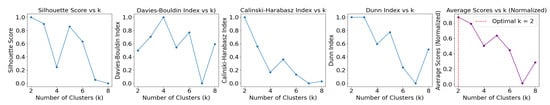
Figure 4.
CVI scores versus the number of clusters. The optimal number of clusters was computed by taking the average of multiple CVI scores after normalization. Figures should be placed in the main text near the first time they are cited.
3.2. Results from Supervised Machine Learning
The fuzzy membership matrix U corresponding to the optimal cluster center k = 2 was combined with class label values from the DARWIN dataset to train supervised learning algorithms. We conducted two sets of experiments: in the first set, we directly applied all ten state-of-the-art supervised learning algorithms to the DARWIN dataset, without utilizing FCM as Stage 1. In the second experiment set, we applied the same algorithms after performing Stage 1 with FCM.
During the first experiment set, we investigated the performance of the supervised learning algorithms in isolation, without leveraging the preliminary clustering insights provided by FCM. This approach allowed us to discern the inherent capabilities and limitations of each algorithm in its raw form, providing valuable insights into their individual efficacy in handling the handwriting data.
In contrast, the second experiment set aimed to capitalize on the initial clustering performed by FCM in Stage 1. By incorporating the fuzzy membership matrix U as features alongside the class labels, we provided the supervised learning algorithms with a richer and more nuanced input space. This augmentation facilitated the algorithms in capturing subtle patterns and relationships within the data, potentially enhancing their predictive performance.
A comparative analysis between the two experiment sets enabled us to gain deeper insights into the interplay between clustering and supervised learning in the context of Alzheimer’s disease diagnosis through handwriting analysis. By systematically evaluating the performance of the algorithms under different experimental conditions, we aimed to uncover optimal synergies between unsupervised clustering and subsequent supervised learning phases, with the ultimate goal of improving diagnostic accuracy and effectiveness.
3.2.1. Applying Classifiers Without Stage 1 (FCM)
In this series of experiments, we initiated our exploration with a grid-search cross-validation method, prioritizing accuracy as the primary performance criterion, to meticulously identify the optimal hyperparameter values for each of the supervised learning algorithms. Utilizing the DARWIN dataset enriched with clinical features, we embarked on an exhaustive exploration aimed at refining the algorithms’ configurations. The detailed results of these experiments are meticulously documented in Table 6, encapsulating a total of 12,310 trials, executed with precision to pinpoint the optimal settings for the ten supervised learning algorithms under scrutiny.
Table 6.
Structure and components of a typical confusion matrix.
Of particular interest, it was revealed that the Support Vector Machine (SVM) algorithm attained the highest accuracy score, reaching an impressive 91%. This notable achievement was realized with a specific hyper-parameter configuration, with ‘C’ set to 1, ‘gamma’ set to ‘scale’, and ‘kernel’ set to ‘rbf’. Following this discovery, we proceeded to conduct a rigorous comparison of all classifiers, employing seven performance evaluation metrics to comprehensively assess their efficacy.
To further validate the robustness of our findings and ensure the generalizability of the observed trends, we undertook a 10-fold cross-validation procedure. This meticulous validation process involved utilizing the specific optimal hyperparameter values identified through the grid-search method. The outcomes of this 10-fold cross-validation experiment are meticulously outlined in Table 7, providing deeper insights into the classifiers’ performance across multiple evaluation metrics.
Table 7.
Determining optimal hyperparameter for different algorithms using Grid Search CV, without stage 1.
Noteworthy among all classifiers considered were Random Forest (RF), Extra Trees (ET), Gaussian Naive Bayes (GNB), and XGBoost (XGB), which consistently exhibited superior performance across the evaluation metrics. These algorithms demonstrated remarkable robustness and efficacy in capturing the intricate patterns inherent in the DARWIN dataset. It is important to highlight that the XGBoost (XGB) classifier achieved the highest mean accuracy of 86%, even without employing Stage 1, the preliminary clustering with Fuzzy C Means.
This extensive experimentation and validation process not only contributed to refining the optimal hyperparameter configurations for each algorithm but also offered valuable insights into their comparative performance under stringent evaluation conditions. By meticulously assessing their performance using both grid-search cross-validation and 10-fold cross-validation, we ensured a comprehensive evaluation of their generalization capabilities and effectiveness in the complex task of handwriting-based Alzheimer’s disease diagnosis.
3.2.2. Applying Classifiers with Stage 1 (FCM)
In this comprehensive series of experiments, we meticulously employed all ten state-of-the-art supervised learning algorithms previously mentioned, leveraging the cognitive dataset generated in Stage 1 as the foundation for our analysis. To discern the optimal configuration of the algorithms’ hyperparameters, we once again turned to the Grid-Search-CV method, meticulously exploring a myriad of parameter combinations to achieve optimal performance. The detailed results of this hyperparameter tuning process are thoughtfully presented in Table 8, offering a comprehensive overview of the optimized settings for each algorithm.
Table 8.
Performance metrics for all the classifiers using 10-fold cross validation, without stage 1.
Building upon the insights gleaned from the hyperparameter tuning phase, we proceeded to conduct a rigorous evaluation of each algorithm’s performance using 10-fold cross-validation. This meticulous validation approach allowed us to robustly assess the algorithms’ predictive capabilities and generalization performance across different subsets of the dataset. The outcomes of these validation experiments are meticulously documented in Table 9, offering a detailed glimpse into each algorithm’s performance metrics and highlighting their respective strengths and weaknesses. Figure 5 displays the AUC-ROC for each fold, as well as the micro-average and macro-average ROC curves for the Decision Tree (DT), Random Forest (RF), Extra Tree (ET), and K-nearest-neighbor (KNN) classifiers. AUC-ROC curves for all other classifiers are presented in the Supplementary Materials.
Table 9.
Determining optimal hyperparameters for the different algorithms using Grid-Search CV, with stage 1.
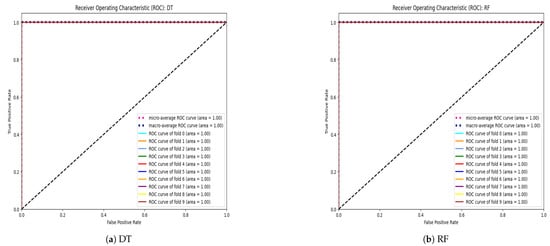
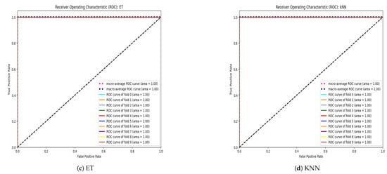
Figure 5.
AUC-ROC curves for each fold, along with micro-average and macro-average ROC curves for (a) Decision Tree (DT), (b) Random Forest (RF), (c) Extra Trees (ET), and (d) k-Nearest Neighbors (KNNs).
Of particular note, the tree-based classifiers, including Decision Trees (DT), Random Forests (RF), and Extra Trees (ET), emerged as the standout performers in terms of predictive accuracy and robustness. These algorithms showcased exceptional performance across the various evaluation metrics, underscoring their efficacy in handling the complexities inherent in the AD diagnosis task.
Interestingly, a notable observation emerged from our analysis: all classifiers, with the exception of Logistic Regression (LR) and Multi-layer Perceptron (MLP), demonstrated a significant enhancement in their predictive capabilities when leveraging the insights gained from Fuzzy C Means (FCM) clustering at Stage 1 (Figure 6). This finding highlights the invaluable role of unsupervised clustering in augmenting the predictive power of supervised learning algorithms, particularly in the context of AD diagnosis through handwriting analysis.
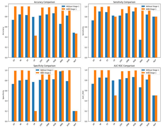
Figure 6.
Comparative performance of the base line classifiers, with and without stage 1.
In summary, our meticulous experimentation and rigorous validation procedures provided valuable insights into the optimal configuration and performance of supervised learning algorithms in the domain of AD diagnosis. By systematically exploring different algorithmic configurations and leveraging the synergies between unsupervised clustering and supervised learning, we have laid a solid foundation for future advancements in this critical area of research.
3.3. Comparative Performance
Furthermore, we conducted an extensive comparative analysis with previously reported approaches focused on predicting Alzheimer’s disease utilizing the DARWIN dataset. The outcomes from these studies are meticulously detailed in Table 10, providing a comprehensive side-by-side comparison with the results obtained from our proposed models (Table 11). Notably, the integration of the unsupervised algorithm Fuzzy C Means (FCM) with the supervised Random Forest (RF) algorithm led to a significant enhancement in overall predictive performance. This noteworthy improvement underscored the effectiveness of synergizing the strengths of a hybrid model, harnessing both unsupervised and supervised learning paradigms to achieve superior predictive accuracy.
Table 10.
Performance metrics for all the classifiers using 10-fold cross-validation, with stage 1.
Table 11.
Comparative performance with the proposed model.
The success observed in the final results reaffirmed the validity of our comprehensive methodology and underscored the potential for advanced techniques to enhance the predictive capabilities of machine learning models in medical research and diagnostic applications. By leveraging the complementary strengths of unsupervised clustering and supervised learning, our hybrid approach demonstrated potential for advancing the state-of-the-art in Alzheimer’s disease prediction. This innovative methodology opens new avenues for research and underscores the importance of interdisciplinary collaboration in tackling complex medical challenges.
4. Conclusions, Limitations, and Future Work
This study successfully developed a hybrid predictor model for Alzheimer’s disease (AD) using handwriting analysis and machine learning techniques, ensuring both robustness and accuracy. The model operates in two stages: initially employing unsupervised clustering, specifically the Fuzzy C-Mean algorithm, to cluster handwriting samples. Fuzzy logic, chosen for its robust ability to handle data uncertainties, is particularly well-suited for medical diagnosis, where precision, adaptability, and the ability to manage ambiguous or overlapping symptoms are crucial for accurate decision-making. The study employed four widely used Cluster Validity Indices to qualify the clustering from FCM and determine optimal cluster centers. The fuzzy membership matrix, treating each cluster as a feature with membership degrees as values, transitioned to the supervised stage for predictor model development. This two-stage model significantly enhanced the performance in detecting AD patients, achieving a mean accuracy of 99%, mean sensitivity of 98%, mean specificity of 100%, mean precision of 100%, and mean MCC and Cohen’s Kappa of 98%, along with a mean AUC-ROC score of 99%. Notably, integrating unsupervised cognition with supervised learning using FCM in the first stage improved the classifier performance by 12% to 26%, highlighting the importance of this integration.
Despite these promising results, this study has certain limitations. First, handwriting variability due to external factors such as age, education level, or underlying health conditions was not thoroughly analyzed. These factors may influence the model’s effectiveness and should be explored in future research. Additionally, the model was tested on a relatively small group of 174 participants, raising concerns about its generalizability to a larger population. A more extensive and diverse dataset is required to validate the model’s performance across different demographic groups.
To address these limitations, future work will focus on expanding the dataset by implementing the protocol proposed by Cilia et al. [], collecting additional handwriting samples from both healthy individuals and AD patients. This will improve the model’s robustness and enhance its applicability in real-world clinical settings. Furthermore, the model could be deployed as software for mobile devices and embedded systems, facilitating easy access for practitioners and supporting early diagnosis in non-clinical environments.
Supplementary Materials
The following supporting information can be downloaded at https://www.mdpi.com/article/10.3390/info16030249/s1, Table S1: List of tasks performed. Task categories are memory and dictation (M), Graphic (G), and Copy (C). Table S2: List of features associated with each tasks.
Author Contributions
Conceptualization, S.U.R. and U.M.; methodology, S.U.R. and U.M.; software, S.U.R. and U.M.; validation, S.U.R. and U.M.; formal analysis, S.U.R. and U.M.; investigation, S.U.R. and U.M.; resources, S.U.R. and U.M.; data curation, U.M.; writing—original draft preparation, S.U.R. and U.M.; writing—review and editing, S.U.R. and U.M.; visualization, S.U.R. and U.M.; supervision, S.U.R.; project administration, S.U.R. All authors have read and agreed to the published version of the manuscript.
Funding
This research received no external funding.
Institutional Review Board Statement
Not applicable.
Informed Consent Statement
Not applicable.
Data Availability Statement
Data are contained within the article.
Acknowledgments
This work was supported in part by Kingdom University, Bahrain, under Grant KU–SRU–2024–13.
Conflicts of Interest
The authors declare no conflicts of interest.
References
- Available online: https://www.who.int/news-room/fact-sheets/detail/dementia (accessed on 13 November 2023).
- Singhal, A.K.; Naithani, V.; Bangar, O.P. Medicinal plants with a potential to treat Alzheimer and associated symptoms. Int. J. Nutr. Pharmacol. Neurol. Dis. 2012, 2, 84–91. [Google Scholar] [CrossRef]
- Armstrong, M.J.; Litvan, I.; Lang, A.E.; Bak, T.H.; Bhatia, K.P.; Borroni, B.; Boxer, A.L.; Dickson, D.W.; Grossman, M.; Hallett, M.; et al. Criteria for the diagnosis of corticobasal degeneration. Neurology 2013, 80, 496–503. [Google Scholar] [CrossRef] [PubMed]
- Duranti, E.; Villa, C. From Brain to Muscle: The Role of Muscle Tissue in Neurodegenerative Disorders. Biology 2024, 13, 719. [Google Scholar] [CrossRef]
- Saxton, J.; Lopez, O.L.; Ratcliff, G.; Dulberg, C.; Fried, L.P.; Carlson, M.C.; Newman, A.B.; Kuller, L. Preclinical Alzheimer disease: Neuropsychological test performance 1.5 to 8 years prior to onset. Neurology 2004, 63, 2341–2347. [Google Scholar] [CrossRef]
- Rasmussen, J.; Langerman, H. Alzheimer’s disease–why we need early diagnosis. Degener. Neurol. Neuromuscul. Dis. 2019, 9, 123–130. [Google Scholar] [CrossRef] [PubMed]
- Cilia, N.D.; De Stefano, C.; Fontanella, F.; Di Freca, A.S. An experimental protocol to support cognitive impairment diagnosis by using handwriting analysis. Procedia Comput. Sci. 2018, 141, 466–471. [Google Scholar] [CrossRef]
- Nichols, E.; Steinmetz, J.D.; Vollset, S.E.; Fukutaki, K.; Chalek, J.; Abd-Allah, F.; Abdoli, A.; Abualhasan, A.; Abu-Gharbieh, E.; Akram, T.T.; et al. Estimation of the global prevalence of dementia in 2019 and forecasted prevalence in 2050: An analysis for the Global Burden of Disease Study 2019. Lancet Public Health 2022, 7, e105–e125. [Google Scholar] [CrossRef]
- Available online: https://pubmed.ncbi.nlm.nih.gov/38689398/ (accessed on 15 March 2025).
- Available online: https://pubmed.ncbi.nlm.nih.gov/33667416/ (accessed on 15 March 2025).
- Reisberg, B.; Ferris, S.H.; de Leon, M.J.; Crook, T. The Global Deterioration Scale for assessment of primary degenerative dementia. Am. J. Psychiatry 1982, 139, 1136–1139. [Google Scholar]
- Precup, R.E.; Teban, T.A.; Albu, A.; Borlea, A.B.; Zamfirache, I.A.; Petriu, E.M. Evolving fuzzy models for prosthetic hand myoelectric-based control. IEEE Trans. Instrum. Meas. 2020, 69, 4625–4636. [Google Scholar] [CrossRef]
- Myszczynska, M.A.; Ojamies, P.N.; Lacoste, A.M.; Neil, D.; Saffari, A.; Mead, R.; Hautbergue, G.M.; Holbrook, J.D.; Ferraiuolo, L. Applications of machine learning to diagnosis and treatment of neurodegenerative diseases. Nat. Rev. Neurol. 2020, 16, 440–456. [Google Scholar] [CrossRef]
- Belić, M.; Bobić, V.; Badža, M.; Šolaja, N.; Đurić-Jovičić, M.; Kostić, V.S. Artificial intelligence for assisting diagnostics and assessment of Parkinson’s disease—A review. Clin. Neurol. Neurosurg. 2019, 184, 105442. [Google Scholar] [CrossRef] [PubMed]
- Scott, I.; Carter, S.; Coiera, E. Clinician checklist for assessing suitability of machine learning applications in healthcare. BMJ Health Care Inform. 2021, 28, e100251. [Google Scholar] [CrossRef] [PubMed]
- Ranjan, N.; Kumar, D.U.; Dongare, V.; Chavan, K.; Kuwar, Y. Diagnosis of Parkinson disease using handwriting analysis. Int. J. Comput. Appl. 2022, 184, 13–16. [Google Scholar]
- Pozna, C.; Precup, R.E. Applications of signatures to expert systems modelling. Acta Polytech. Hung. 2014, 11, 21–39. [Google Scholar]
- Pirlo, G.; Diaz, M.; Ferrer, M.A.; Impedovo, D.; Occhionero, F.; Zurlo, U. Early diagnosis of neurodegenerative diseases by handwritten signature analysis. In New Trends in Image Analysis and Processing—Proceedings of the ICIAP 2015 Workshops: ICIAP 2015 International Workshops, BioFor, CTMR, RHEUMA, ISCA, MADiMa, SBMI, and QoEM, Genoa, Italy, 7–8 September 2015; Proceedings 18; Springer International Publishing: Berlin/Heidelberg, Germany, 2015; pp. 290–297. [Google Scholar]
- Senatore, R.; Marcelli, A. A paradigm for emulating the early learning stage of handwriting: Performance comparison between healthy controls and Parkinson’s disease patients in drawing loop shapes. Hum. Mov. Sci. 2019, 65, 89–101. [Google Scholar] [CrossRef]
- Xie, L.; Das, S.R.; Wisse, L.E.; Ittyerah, R.; de Flores, R.; Shaw, L.M.; Yushkevich, P.A.; Wolk, D.A.; Alzheimer’s Disease Neuroimaging Initiative. Baseline structural MRI and plasma biomarkers predict longitudinal structural atrophy and cognitive decline in early Alzheimer’s disease. Alzheimer’s Res. Ther. 2023, 15, 79. [Google Scholar] [CrossRef]
- Abbas, S.Q.; Chi, L.; Chen, Y.P.P. Transformed domain convolutional neural network for alzheimer’s disease diagnosis using structural MRI. Pattern Recognit. 2023, 133, 109031. [Google Scholar] [CrossRef]
- Wang, J.; Jin, C.; Zhou, J.; Zhou, R.; Tian, M.; Lee, H.J.; Zhang, H. PET molecular imaging for pathophysiological visualization in Alzheimer’s disease. Eur. J. Nucl. Med. Mol. Imaging 2023, 50, 765–783. [Google Scholar] [CrossRef]
- Rallabandi, V.S.; Seetharaman, K. Deep learning-based classification of healthy aging controls, mild cognitive impairment and Alzheimer’s disease using fusion of MRI-PET imaging. Biomed. Signal Process. Control 2023, 80, 104312. [Google Scholar]
- Kaya, M.; Çetin-Kaya, Y. A Novel Deep Learning Architecture Optimization for Multiclass Classification of Alzheimer’s Disease Level. IEEE Access 2024, 12, 46562–46581. [Google Scholar] [CrossRef]
- Rehman, S.U.; Tarek, N.; Magdy, C.; Kamel, M.; Abdelhalim, M.; Melek, A.; Mahmoud, L.N.; Sadek, I. AI-based tool for early detection of Alzheimer’s disease. Heliyon 2024, 10, e29375. [Google Scholar] [CrossRef]
- Ahmed, H.; Soliman, H.; Elmogy, M. Early detection of Alzheimer’s disease using single nucleotide polymorphisms analysis based on gradient boosting tree. Comput. Biol. Med. 2022, 146, 105622. [Google Scholar] [CrossRef] [PubMed]
- Yin, W.; Yang, T.; Wan, G.; Zhou, X. Identification of image genetic biomarkers of Alzheimer’s disease by orthogonal structured sparse canonical correlation analysis based on a diagnostic information fusion. Math. Biosci. Eng. 2023, 20, 16648–16662. [Google Scholar] [CrossRef] [PubMed]
- Chen, Y.; Sun, Y.; Luo, Z.; Chen, X.; Wang, Y.; Qi, B.; Lin, J.; Lin, W.W.; Sun, C.; Zhou, Y.; et al. Exercise modifies the transcriptional regulatory features of monocytes in Alzheimer’s patients: A multi-omics integration analysis based on single cell technology. Front. Aging Neurosci. 2022, 14, 881488. [Google Scholar] [CrossRef]
- Jiao, B.; Li, R.; Zhou, H.; Qing, K.; Liu, H.; Pan, H.; Lei, Y.; Fu, W.; Wang, X.; Xiao, X.; et al. Neural biomarker diagnosis and prediction to mild cognitive impairment and Alzheimer’s disease using EEG technology. Alzheimer’s Res. Ther. 2023, 15, 32. [Google Scholar] [CrossRef] [PubMed]
- Hou, Q.; Guan, Y.; Liu, X.; Xiao, M.; Lü, Y. Development and validation of a risk model for cognitive impairment in the older Chinese inpatients: An analysis based on a 5-year database. J. Clin. Neurosci. 2022, 104, 29–33. [Google Scholar] [CrossRef]
- Odusami, M.; Maskeliūnas, R.; Damaševičius, R.; Misra, S. Machine learning with multimodal neuroimaging data to classify stages of Alzheimer’s disease: A systematic review and meta-analysis. Cogn. Neurodyn. 2023, 18, 775–794. [Google Scholar] [CrossRef]
- Qiu, S.; Miller, M.I.; Joshi, P.S.; Lee, J.C.; Xue, C.; Ni, Y.; Wang, Y.; De Anda-Duran, I.; Hwang, P.H.; Cramer, J.A.; et al. Multimodal deep learning for Alzheimer’s disease dementia assessment. Nat. Commun. 2022, 13, 3404. [Google Scholar] [CrossRef]
- Accardo, A.; Chiap, A.; Borean, M.; Bravar, L.; Zoia, S.; Carrozzi, M.; Scabar, A. A device for quantitative kinematic analysis of children’s handwriting movements. In Proceedings of the 11th Mediterranean Conference on Medical and Biomedical Engineering and Computing 2007: MEDICON 2007, Ljubljana, Slovenia, 26–30 June 2007; Springer: Berlin/Heidelberg, Germany, 2007; pp. 445–448. [Google Scholar]
- De Stefano, C.; Fontanella, F.; Impedovo, D.; Pirlo, G.; di Freca, A.S. Handwriting analysis to support neurodegenerative diseases diagnosis: A review. Pattern Recognit. Lett. 2019, 121, 37–45. [Google Scholar] [CrossRef]
- Vessio, G. Dynamic handwriting analysis for neurodegenerative disease assessment: A literary review. Appl. Sci. 2019, 9, 4666. [Google Scholar] [CrossRef]
- Singh, P.; Yadav, H. Influence of neurodegenerative diseases on handwriting. Forensic Res. Criminol. Int. J. 2021, 9, 110–114. [Google Scholar] [CrossRef]
- Impedovo, D.; Pirlo, G.; Vessio, G.; Angelillo, M.T. A handwriting-based protocol for assessing neurodegenerative dementia. Cogn. Comput. 2019, 11, 576–586. [Google Scholar] [CrossRef]
- Impedovo, D.; Pirlo, G.; Vessio, G. Dynamic handwriting analysis for supporting earlier Parkinson’s disease diagnosis. Information 2018, 9, 247. [Google Scholar] [CrossRef]
- Cavallo, F.; Moschetti, A.; Esposito, D.; Maremmani, C.; Rovini, E. Upper limb motor pre-clinical assessment in Parkinson’s disease using machine learning. Park. Relat. Disord. 2019, 63, 111–116. [Google Scholar] [CrossRef]
- De Gregorio, G.; Desiato, D.; Marcelli, A.; Polese, G. A multi classifier approach for supporting Alzheimer’s diagnosis based on handwriting analysis. In Proceedings of the Pattern Recognition. ICPR International Workshops and Challenges, Virtual Event, 10–15 January 2021; Proceedings, Part I. Springer International Publishing: Berlin/Heidelberg, Germany, 2021; pp. 559–574. [Google Scholar]
- Cilia, N.D.; De Gregorio, G.; De Stefano, C.; Fontanella, F.; Marcelli, A.; Parziale, A. Diagnosing Alzheimer’s disease from on-line handwriting: A novel dataset and performance benchmarking. Eng. Appl. Artif. Intell. 2022, 111, 104822. [Google Scholar] [CrossRef]
- Parziale, A.; Della Cioppa, A.; Marcelli, A. Investigating one-class classifiers to diagnose Alzheimer’s disease from handwriting. In Proceedings of the International Conference on Image Analysis and Processing, Lecce, Italy, 23–27 May 2022; Springer International Publishing: Cham, Switzerland, 2022; pp. 111–123. [Google Scholar]
- Subha, R.; Nayana, B.R.; Selvadass, M. Hybrid Machine Learning Model Using Particle Swarm Optimization for Effectual Diagnosis of Alzheimer’s Disease from Handwriting. In Proceedings of the 2022 4th International Conference on Circuits, Control, Communication and Computing (I4C), Bangalore, India, 21–23 December 2022; IEEE: Piscataway, NJ, USA, 2022; pp. 491–495. [Google Scholar]
- Gattulli, V.; Impedovo, D.; Semeraro, G.P.G. Handwriting Task-Selection based on the Analysis of Patterns in Classification Results on Alzheimer Dataset. DSTNDS 2023, 18–29. [Google Scholar]
- Önder, M.; Şentürk, Ü.; Polat, K.; Paulraj, D. Diagnosis of Alzheimer’s Disease Using Boosting Classification Algorithms. In Proceedings of the 2023 International Conference on Research Methodologies in Knowledge Management, Artificial Intelligence and Telecommunication Engineering (RMKMATE), Chennai, India, 1–2 November 2023; IEEE: Piscataway, NJ, USA, 2023; pp. 1–5. [Google Scholar]
- Hakan, Ö.C.A.L. A Novel Approach to Detection of Alzheimer’s Disease from Handwriting: Triple Ensemble Learning Model. Gazi Univ. J. Sci. Part C Des. Technol. 2024, 12, 214–223. [Google Scholar]
- Mitra, U.; Rehman, S.U. ML-Powered Handwriting Analysis for Early Detection of Alzheimer’s Disease. IEEE Access 2024, 12, 69031–69050. [Google Scholar] [CrossRef]
- Erdogmus, P.; Kabakus, A.T. The promise of convolutional neural networks for the early diagnosis of the Alzheimer’s disease. Eng. Appl. Artif. Intell. 2023, 123, 106254. [Google Scholar] [CrossRef]
- Rousseeuw, P.J. Silhouettes: A graphical aid to the interpretation and validation of cluster analysis. J. Comput. Appl. Math. 1987, 20, 53–65. [Google Scholar] [CrossRef]
- Davies, D.L.; Bouldin, D.W. A cluster separation measure. IEEE Trans. Pattern Anal. Mach. Intell. 1979, 224–227. [Google Scholar] [CrossRef]
- Caliński, T.; Harabasz, J. A dendrite method for cluster analysis. Commun.-Stat.-Theory Methods 1974, 3, 1–27. [Google Scholar] [CrossRef]
- Bezdek, J.C.; Pal, N.R. Some new indexes of cluster validity. IEEE Trans. Syst. Man Cybern. Part B (Cybern.) 1998, 28, 301–315. [Google Scholar] [CrossRef] [PubMed]
- Nasteski, V. An overview of the supervised machine learning methods. Horizons b 2017, 4, 56. [Google Scholar] [CrossRef]
Disclaimer/Publisher’s Note: The statements, opinions and data contained in all publications are solely those of the individual author(s) and contributor(s) and not of MDPI and/or the editor(s). MDPI and/or the editor(s) disclaim responsibility for any injury to people or property resulting from any ideas, methods, instructions or products referred to in the content. |
© 2025 by the authors. Licensee MDPI, Basel, Switzerland. This article is an open access article distributed under the terms and conditions of the Creative Commons Attribution (CC BY) license (https://creativecommons.org/licenses/by/4.0/).