Article

A Method for Improving the Monitoring Quality and Network Lifetime of Hybrid Self-Powered Wireless Sensor Networks

1
School of Automation, China University of Geosciences, Wuhan 430074, China
2
Hubei Key Laboratory of Advanced Control and Intelligent Automation for Complex Systems, Wuhan 430074, China
3
Engineering Research Center of Intelligent Technology for Geo-Exploration, Ministry of Education, Wuhan 430074, China
*
Author to whom correspondence should be addressed.
Information 2025, 16(3), 228; https://doi.org/10.3390/info16030228
Submission received: 23 January 2025 / Revised: 12 March 2025 / Accepted: 13 March 2025 / Published: 15 March 2025

Abstract

:
Wireless sensors deployed in large agricultural areas can monitor and collect data in real time, helping to achieve smart agriculture. But the complexity of the environment and the random deployment method seriously affect the coverage quality. The limited capacity of sensor batteries greatly limits the network lifetime. Therefore, how to extend the network lifetime while ensuring coverage quality is a highly challenging task. This paper proposes a node deployment optimization method to solve the problems of a poor coverage rate and a short network lifetime in hybrid self-powered sensor networks in obstacle environments. This method first optimizes the sensing direction of stationary nodes, expands the coverage range, and repairs coverage holes. Then, an improved bidirectional search A* algorithm is used to plan the obstacle avoidance moving path of mobile nodes, fill the remaining coverage holes, and improve the coverage quality of the network. Finally, a method based on an improved nutcracker optimizer algorithm is proposed to solve the optimal working sequence of nodes, schedule the “sleep or work” state of nodes, and extend the network lifetime. The simulation experiment verified the effectiveness of the proposed method, indicating that its performance in coverage quality, mobile energy consumption, and network lifetime is superior to other compared methods.

Graphical Abstract

1. Introduction

Wireless sensor networks (WSNs) are the foundation and core of the sensing layer in the Internet of Things. The different types of sensors deployed in the sensing layer can collect and transmit various required data. Currently, WSNs play an important role in many industries, including intelligent transportation, ecological monitoring, forest protection, and smart agriculture [1,2]. However, in practical applications, there are still some issues that need to be addressed, such as coverage hole and monitoring time. Random deployment, environmental factors, and electronic component failures can all lead to some areas in the monitoring area not being covered by sensors, resulting in coverage holes and affecting coverage quality [3]. In addition, redundant coverage in the network and energy limitations of sensors significantly affect the network lifetime, making it impossible to meet the requirements of long-term monitoring. Therefore, repairing coverage holes to achieve coverage enhancement is a key task in improving monitoring quality. Reducing redundancy, the rational use of energy, and extending the network lifetime are other highly challenging tasks.
Coverage holes can lead to the omission of important information and interruption of network connections, seriously affecting the overall performance of the network. It is reasonable and necessary to improve coverage quality by scheduling nodes to repair holes and enhance coverage. For omnidirectional sensors, the method to repair coverage holes is achieved by moving the sensor. In directional sensor networks, we typically use intelligent optimization algorithms such as ant colony, particle swarm, and genetic algorithms to adjust sensing direction and schedule mobile nodes [4,5,6]. Compared to other methods, the advantages of these methods are fewer parameters and faster computation speed. The existing research work mainly focuses on ideal environments and rarely considers the influence of terrain and obstacles. A lack of consideration for environmental factors can make existing methods difficult to apply in practical scenarios.
The limited lifetime of networks is an important issue that constrains the quality of wireless sensor network services [7]. The limited capacity of sensor batteries and unreasonable energy usage are the two major factors that limit the network lifetime [8]. There are four main methods for extending a network lifetime: network clustering, sleep–work strategy, self-powered energy harvesting, and mobile charging [9,10]. Among them, network clustering and sleep–work strategies both extend the network lifetime through energy-saving methods and cannot generate new energy [11]. So their effectiveness is not as good as the other two methods. The conditions required for mobile charging methods are much higher than those for energy harvesting technology [12]. The existing research on self-powered (energy harvesting) sensor networks mostly adopts omnidirectional sensing models and rarely considers the impact of environmental factors (lighting, temperature) on charging efficiency. It is very important to comprehensively consider the influencing factors in the real environment to enhance the applicability of energy harvesting networks.
To sum up, we find that existing methods for enhancing coverage and extending network lifetime have certain limitations. In current coverage enhancement research, researchers rarely consider the impact of obstacles on node movement. Obstacles are commonly present in outdoor environments. Introducing self-powered sensors is a good method to extend the network lifetime. Self-powered sensors store energy by collecting solar energy. The weather conditions have a significant impact on the efficiency of sensors collecting solar energy. The lack of consideration for environmental factors is a limitation of existing energy harvesting methods. In addition, after introducing self-powered sensors, we should also consider how to schedule nodes to reduce sensor usage and further increase the remaining energy of the network.
Based on the above analysis, we studied the monitoring quality and network lifetime problems of hybrid self-powered wireless sensor networks and proposed a node deployment optimization method. The hybrid self-powered wireless sensor network consists of stationary non-rechargeable nodes and mobile rechargeable nodes. In the proposed method, we considered the limitations of obstacles on node movement and also measured the impact of environmental factors on sensor energy collection. The proposed method first solves the optimal set of sensing directions for stationary nodes and repairs some coverage holes. Then, an improved bidirectional A* algorithm is used to search the obstacle avoidance moving path of nodes and fill the remaining coverage holes. Finally, a network lifetime optimization model is established with the optimization objectives of maximizing the residual energy of the network and minimizing the required number of sensors, and an improved nutcracker optimizer algorithm is used for solving. Arrange the working sequence of nodes based on the obtained subset of nodes, reduce the sensing energy consumption of nodes, and prolong the network lifetime. The major contributions of our research can be summarized as follows.
  • This paper proposes a node deployment optimization method based on node sensing direction, location, and working state optimization to solve the problems of coverage quality and network lifetime in obstacle environments. This method improves coverage quality by repairing coverage holes and extends network lifetime through node sleep scheduling.
  • We have designed a coverage quality enhancement method based on repairing coverage holes. This method first optimizes the sensing direction of stationary nodes and repairs coverage holes that are closer in distance. Then, an improved bidirectional A* algorithm is used to determine the shortest obstacle avoidance moving path, repair the remaining coverage holes, and improve the coverage quality of the network.
  • We established a network lifetime optimization model with the residual energy and required number of sensors as targets and used an improved nutcracker optimizer algorithm to solve it. By scheduling the working status of nodes based on the optimal subset obtained, energy consumption can be reduced, thereby extending the network lifetime.
  • We designed several simulation experiments to demonstrate the performance of the proposed method in coverage quality, mobile energy consumption, and network lifetime. The comparison with other advanced algorithms proves the effectiveness and superiority of the proposed algorithm.
The rest of this paper is arranged as follows: In Section 2, we provide a detailed introduction to the related work on coverage enhancement and node scheduling problems. The system model and problem description are presented in Section 3. Section 4 introduces the proposed algorithms. The evaluation results of algorithm performance are presented in Section 5. We summarize the work of this paper and plan for future work in Section 6.

2. Related Work

Coverage enhancement and network lifetime extension are important problems in WSNs, and they are also the focus of current research. In this section, we describe in detail how to achieve coverage enhancement and extend the lifetime of the network.

2.1. Coverage Enhancement Method Based on Repairing Coverage Holes

Coverage enhancement is an important method to improve network coverage quality and is currently a research hotspot. Usually, coverage enhancement is achieved by repairing coverage holes. There are two main methods to repair coverage holes: mobile node location update (for omnidirectional sensing model) and optimizing the sensing direction or the location of nodes (for directional sensing model) [13,14]. Intelligent optimization algorithms are important methods for solving the above two types of problems. Yao et al. [15] established a node sensing direction scheduling model with the objective function of minimizing redundancy. They use the discrete army ant optimization algorithm to optimize the working direction of sensors. The optimal working direction reduces the redundant area and expands the effective coverage area. Therefore, the monitoring quality of the system has been greatly improved. Geometric methods, virtual force algorithms (VFAs), and combinatorial optimization methods are also high-performance solving methods [16]. Chen et al. [17] integrated the virtual force algorithm into the particle swarm optimization algorithm and proposed a new coverage enhancement method. This method analyzes the forces between nodes and uses virtual forces to guide the heuristic algorithm to optimize the working direction of sensors. The optimized sensing direction repairs coverage holes in the network and improves coverage performance.
Scheduling mobile nodes to repair coverage holes is another important coverage enhancement method. Current research mostly uses virtual force algorithms, heuristic algorithms, and methods based on the minimum exposure path (MEP) to schedule mobile nodes. Yao et al. [18] applied the VFA to a 3D WSN and designed a node position update scheme. The advantage of this method is that it can improve coverage with less movement distance. And its limitation lies in the inability to ensure the maximum moving distance of a single sensor. Heuristic algorithms are the most widely used method in scheduling mobile node problems. The artificial bee colony algorithm, genetic algorithm, bat algorithm, etc., can all achieve good results. Wen et al. [19] combined a virtual force algorithm and a bat optimization algorithm to redeploy mobile nodes. They conducted rigorous force analysis and designed the node’s movement strategy. After deploying mobile nodes to new locations, network coverage performance is greatly improved. The MEP-based method determines the movement path of nodes by finding the minimum exposure path. Combining the MEP with heuristic algorithms can schedule mobile nodes to coverage holes. Multiple scheduling can greatly improve coverage rate.
The existing coverage enhancement methods mainly focus on optimizing the coverage effect, with less consideration for energy consumption. In addition, the impact of obstacles is rarely considered when planning the movement path of nodes. Due to the battery capacity limitation of sensors, new coverage holes will soon emerge after enhancing network coverage. Therefore, while enhancing coverage, consideration should also be given regarding how to extend the network lifetime.

2.2. Network Lifetime Extension Method Based on Scheduling Nodes

In a WSN composed of battery-powered sensors, the monitoring time is extended by balancing or reducing the energy expenditure of the sensors. Network clustering and duty cycle methods maximize network lifetimes by reducing communication and sensing the energy consumption of nodes. Network clustering is achieved by selecting cluster heads to reduce communication between ordinary nodes and lower energy consumption [20]. The principle of duty cycle policy is to assign nodes to different subsets, and, then, the nodes in the subset can be scheduled to complete the coverage task [21]. Adjusting the state of sensor nodes (working or sleeping) is another way to extend the network lifetime. Reference [22] aims to achieve energy balance and uses heuristic algorithms to schedule the working status of nodes, thereby extending the network’s lifetime. The above method effectively extends the network lifetime through energy-saving methods. However, the above methods still cannot meet the needs of long-term monitoring.
The energy harvesting technology in self-powered sensors has become a current research hotspot. Self-powered sensors are widely used in systems that require an extended network lifetime. Reference [23] proposes an improved greedy algorithm based on priority with the goal of maximizing the network lifetime. Their method can extend the network lifetime while meeting coverage requirements. Xiong and Lu et al. [24] proposed a hybrid sensor network framework. They proposed a network lifetime extension method based on a multi-objective optimization algorithm. This method extends the network lifetime by repairing coverage holes and adjusting node working status.
The existing coverage enhancement methods mainly focus on expanding the coverage area through scheduling nodes but lack an analysis of environmental factors. In outdoor environments, factors such as weather, terrain, and obstacles have a significant impact on node movement. A node moving strategy needs to be designed based on the actual situation. Unstable solar energy in complex environments can also affect the energy harvesting efficiency of self-powered nodes. Therefore, when studying how to improve the monitoring quality and network lifetime of networks, it is necessary to comprehensively measure the impact of environmental factors in order to design more applicable methods.
To summarize the above content, we propose a new node deployment optimization method to address the challenges of monitoring quality and the network lifetime in obstacle environments. This algorithm improves the monitoring quality of the network by scheduling sensor sensing directions and updating node positions. On this basis, adjust the working state of nodes to increase the remaining energy of each time slot in the network, thereby extending the network lifetime.

3. Problem Statement
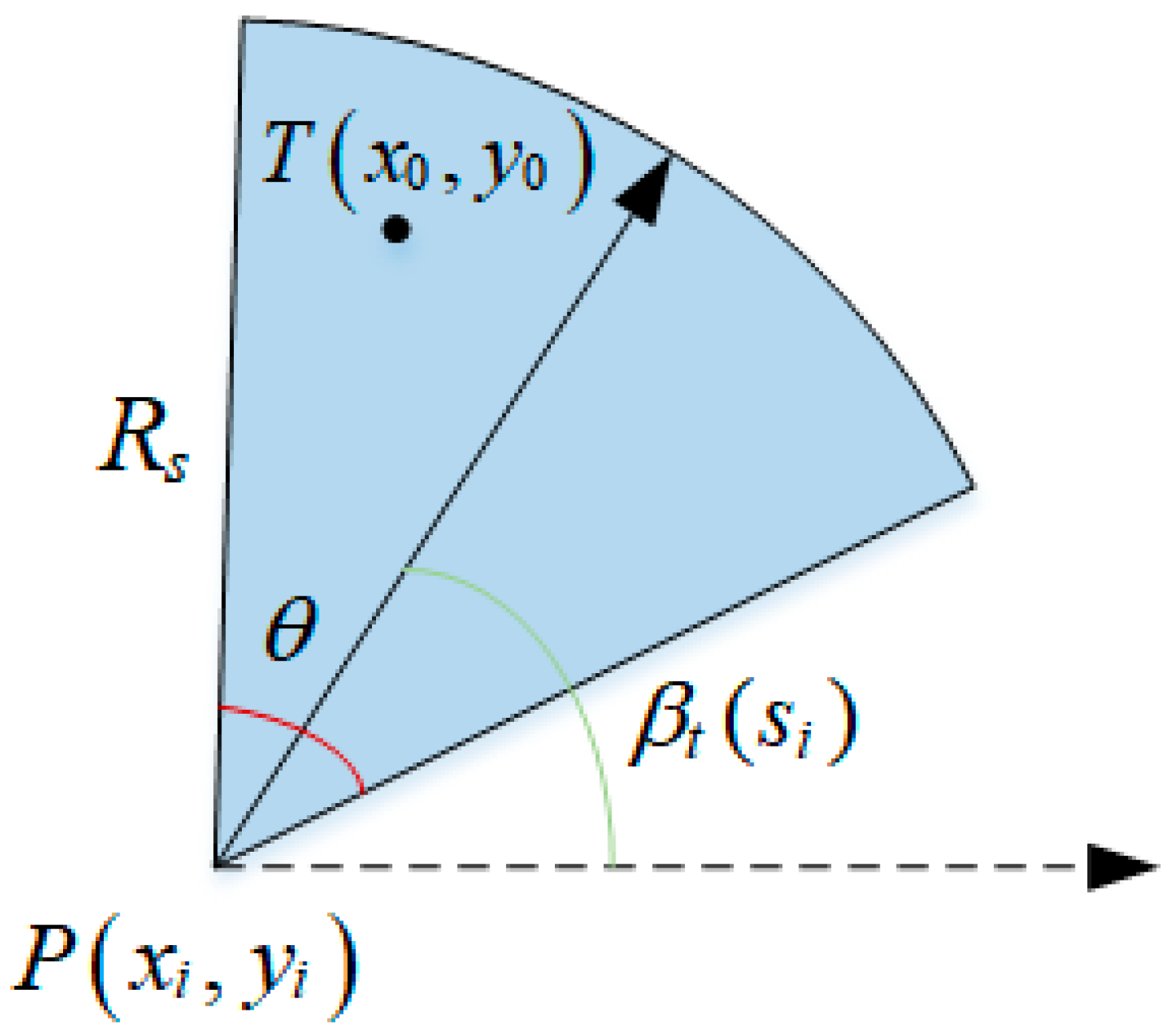
Modeling the research problems is the foundation for designing node deployment optimization methods. This section provides a detailed introduction to the network model, energy consumption model, and node deployment optimization process. Then, the objective function and constraints of the research problem in this paper were stated.

3.1. Network Model

The hybrid self-powered sensor network studied in this paper consists of a certain number of stationary non-rechargeable nodes and mobile rechargeable nodes. Except for the charging characteristics, all node characteristic parameters are completely consistent. We refer to the methods in references [13,14] to ensure node localization and communication and the method described in reference [25] to estimate solar energy intensity and determine charging and discharging rates. In addition, in order to reduce the impact of time delays on inter-node communication, we adopted the method in reference [26] to improve the stability of the system network.
All sensors in this study adopted a directional sensing model and Boolean detection model. The sensing range of a sensor based on a directional sensing model is a sector, and the working direction of the sensor can be changed by rotation. As shown in Figure 1, typically, a 4-tuple is used to represent its sensing model.
P , θ , R s , β t s i
where P = x i , y i represents the position coordinates of the node, θ represents the sensing angle, R s represents the sensing radius, and β t s i represents the current working direction. T = x 0 , y 0 represents the target point located within the sector sensing area.
Since this paper uses a Boolean model, when the target point T = x 0 , y 0 satisfies the following two conditions, it will definitely be detected by the sensor. On the contrary, if the target point T = x 0 , y 0 does not meet these two conditions, it will definitely not be detected.
d i s P , T = x i x 0 2 + y i y 0 2 R S
θ 2 arctan y 0 y i x 0 x i θ 2 + β t s i
The region of interest (ROI) in this paper is a regular rectangle. Its size is L × H . We randomly deploy k targets and n sensor nodes in the ROI. Among them, there are n s stationary sensors and n m mobile sensors. N = n 1 , n 2 , n n , S = s 1 , s 2 , s n s , and M = m 1 , m 2 , m n m , respectively, represent a set of sensors, a set of stationary sensors, and a set of mobile sensors. Stationary sensors can rotate but cannot move or charge. The mobile sensor is rotatable and rechargeable. When the target is within the sensing range of the sensor, the target is covered. If all k targets are covered, then full coverage has been achieved.

3.2. Energy Consumption Model

Self-powered sensors have three states: charging, sensing, and sleep. When performing sensing tasks, sensors consume energy and are in a discharge state. Sleep state does not collect energy or consume energy. The charging rate of sensors is closely related to the solar energy intensity of the day. We imitated the method in reference [25] to estimate the solar energy intensity for that day. Let e s c h a r be the charging rate of the sensor. e s c h a r dynamically changes with the intensity of solar energy.
The energy consumption of sensors in monitoring tasks mainly comes from receiving, transmitting messages, sensing data, and node movement. Let e s m o v e d i s c h be the energy release rate of a node moving a unit distance. The node energy consumption model is shown below:
E C s i = E i s + E i r + E i t + e s m o v e d i s c h × d i s s i
d i s s i = x i f i n a l x i i n i t i 2 + y i f i n a l y i i n i t i 2
where E i s ,   E i r ,   E i t represent the energy consumption of node sensing, reception, and transmission of data, respectively. d i s s i represents the moving distance by the node.

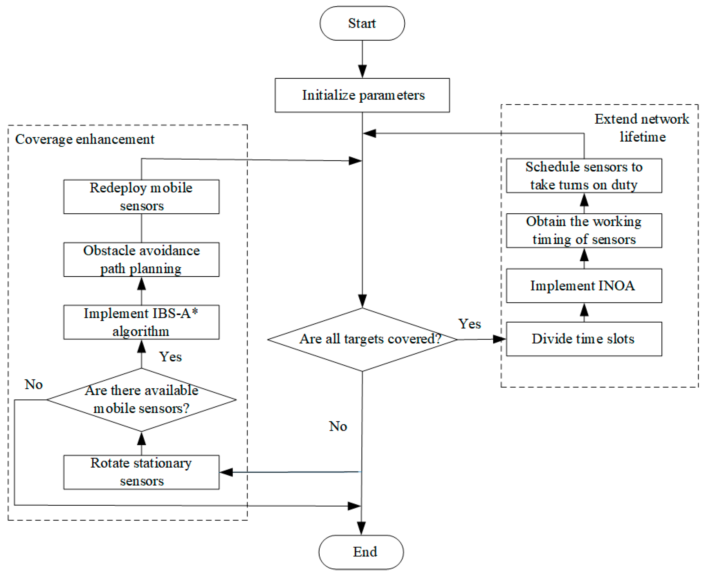
3.3. The Process of Repairing Coverage Holes and Extending Network Lifetime

Repairing coverage holes is the key to achieving coverage enhancement and the first step in extending network lifetime. We repair the holes through two steps: rotating stationary nodes and mobile node relocation.
Figure 2 shows the operation of rotating stationary sensors. There are five targets T 1 T 5 , one obstacle, five stationary non-rechargeable sensors S 1 S 5 , and three mobile rechargeable sensors M 1 M 3 in the monitoring area. The target T 2 T 4 is covered by sensors, and only T 1 ,   T 5 are with coverage holes. S 1 ,   S 5 are in the vicinity of uncovered targets T 1 ,   T 5 . After determining the coverage hole, the stationary sensor is rotated to repair the hole. As shown in the figure, after rotation, the position of S 1 ,   S 5 has changed, and all targets are covered by sensors.
There are two cases for scheduling mobile nodes. Case 1 is shown in Figure 3. There are four targets T 6 T 9 , one obstacle, three stationary non-rechargeable sensors S 6 S 8 , and three mobile rechargeable sensors M 4 M 6 in the monitoring area. Targets T 6 ,   T 8 ,   T 9 are covered by sensors, and only T 7 is a coverage hole. M 5 ,   M 6 are the two closest mobile sensors to the coverage hole. They can all serve as candidate nodes for repairing holes. In order to reduce mobile energy consumption, it is necessary to compare the Euclidean distance between two sensors, and, if d i s M 5 , T 7 < d i s M 6 , T 7 , the mobile node M 5 is chosen to repair the hole. Apart from distance factors, the remaining energy of nodes can also affect the selection of candidate nodes. If the remaining energy is insufficient to meet the requirements, candidate nodes need to be re-selected.
Case 2 is shown in Figure 4. T 10 is the coverage hole, and M 8 ,   M 9 are the two nearest mobile nodes. Firstly, we calculate the distance, denoted as d i s M 8 , T 10 > d i s M 9 , T 10 . But there is an obstacle, and mobile node M 9 cannot move in a straight line to the position of target T 10 . Therefore, we need to recalculate the movement distance of the scheduling nodes. If d i s M 8 , T 10 < d i s M 9 , T 10 , M 8 is the final candidate node.
After coverage enhancement, the monitoring quality of the system has been greatly improved. All target points are covered. However, there is still a problem of redundant coverage in the network. In order to reduce resource waste caused by redundancy, some sensor nodes can be arranged to sleep to reduce unnecessary energy consumption. In any time slot δ i , only one subset that meets the coverage requirements needs to be activated to perform the monitoring task normally. Different subsets need to be activated for different tasks. As shown in Figure 5, in time slot δ i , the working subset is S 1 ,   S 2 ,   M 1 ,   M 2 ,   S 5 ,   S 6 . In time slot δ i + 1 , the working subset is S 1 ,   S 2 ,   M 1 ,   M 3 ,   S 5 ,   S 7 .
Due to some targets being only covered by stationary non-rechargeable nodes, when the energy of the stationary nodes is depleted, this target becomes a coverage hole. In addition, we consider a special case. In the case of the sufficient number of mobile rechargeable nodes, we deploy two mobile nodes at each target by scheduling nodes. When there is only one mobile rechargeable node, the node can only function properly during certain time slots. In the case of deploying two mobile nodes, the nodes can work normally in all time slots.

3.4. Problem Formulation

We achieve coverage enhancement by repairing coverage holes. Then, the network lifetime is extended by scheduling nodes. Next, we analyzed and introduced the objective function of the problem in this paper.

3.4.1. Coverage Enhancement Problem

In the process of implementing coverage enhancement in scheduling nodes, mobile energy consumption is much higher than other energy consumption. Therefore, we choose nodes with smaller moving distances for scheduling. Equation (6) shows the objective function of the coverage enhancement problem.
f 1 = min ( D T o t a l )
s . t . : D T o t a l = i = 1 M d i s m i
z ( m i ) = 0 ,   d i s m i = 0 1 ,   o t h e r w i s e
i = 1 M z m i = Δ n m , i = 1 ,   2 ,   3 ,   M
E m i r e s = E e m i m o v e d i s c h × d i s m i
E m i r e s 0.6 E
where D T o t a l is the total moving distance of all mobile sensors. d i s m i represents the moving distance of a single sensor. z m i is a judgment function. When the moving distance of a node is greater than 0, z m i = 1 . Δ n m represents the number of mobile nodes required to complete the repair of coverage holes, 0 Δ n m n m . M represents the number of available mobile nodes, 0 M n m . E represents the initial energy, e s m o v e d i s c h represents the discharge rate when the node moves, and E m i r e s represents the residual energy.

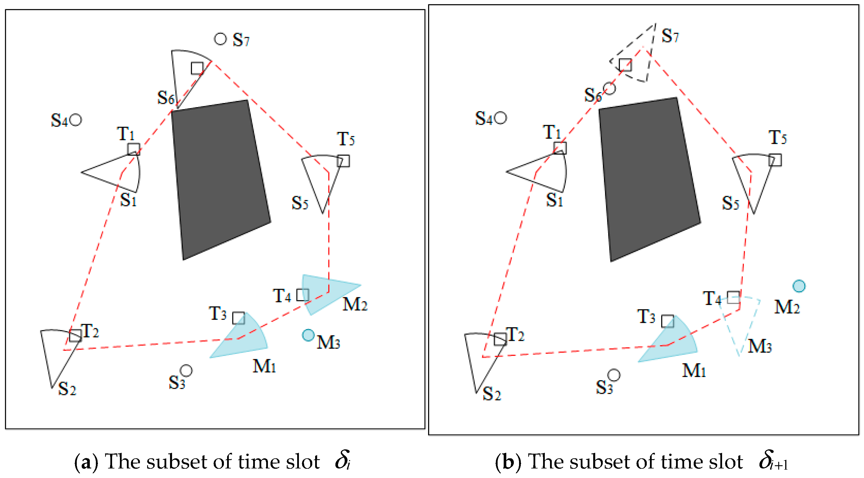
3.4.2. Extended Network Lifetime

Using as few nodes as possible to perform monitoring tasks can reduce unnecessary energy consumption and effectively improve the lifetime of the network. Choosing nodes with more remaining energy is also an effective method. Therefore, the goal of this stage is to increase the remaining energy of each time slot as much as possible, reduce the number of working sensors, and increase the number of charging sensors.
The subset working in the time slot δ i can be represented as N s = N s , 1 ,   N s , 2 ,   N s , 3 ,   N s , k , N s N , and the number of nodes in the subset is shown in the equation.
f 2 = N s
The remaining energy of all nodes in the subset can be expressed as follows:
f 3 = i = 1 k N s , i E r 2 i
where E r 2 i is the remaining energy of the sensor after executing the proposed algorithm. It can be expressed as follows:
E r 2 i = min E r 1 i + σ 1 N s , i μ N s , i δ t , E ,   E r 1 i E t h E r 1 i μ N s , i δ t ,   o t h e r w i s e
where E r 1 i represents the remaining energy after executing the coverage enhancement algorithm, σ , μ are the discharge and charging rates, respectively, and E t h is the energy threshold.
E t h is related to the charging opportunity of the mobile node. Charging begins when the energy is below E t h . The number of mobile nodes charged in the subset can be expressed as follows:
f 4 = N s
Therefore, there are three optimization objectives in the problem of the network lifetime. The optimization model for this problem is shown in Equation (16).
f = min ( f 2 , 1 / f 3 , f 4 )

4. Proposed Method

Our research proposes a new approach to address the challenges of coverage quality and network lifetime in obstacle environments. This method consists of three important steps: rotating stationary nodes; updating the location of mobile nodes and repairing coverage holes; and scheduling node sleep to prolong the network lifetime. Firstly, we determined the geometric length from coverage holes and the stationary nodes and optimized the working direction of nodes that meet the conditions. Then, based on the improved bidirectional search A* algorithm (IBS-A*), the shortest obstacle avoidance moving path was solved, and the position of the mobile node was updated. By optimizing the sensing direction and position of nodes, the task of repairing coverage holes was completed to enhance network coverage. Finally, the improved nutcracker optimizer algorithm (INOA) was used to solve the optimal working sequence of the nodes. Each subset corresponds to a time period. This method avoids unnecessary energy waste and can extend the lifetime of the network. Figure 6 shows the framework and steps of our method.

4.1. Node Scheduling Method for Enhancing Coverage in Obstacle Environments

There are some uncovered targets in the randomly deployed monitoring area. These uncovered targets are coverage holes in the WSN. We improved monitoring quality by repairing coverage holes. The method for repairing coverage holes in this paper includes two parts: rotating stationary nodes and repositioning mobile nodes. Firstly, rotate the stationary sensors around the uncovered target to repair the coverage hole. Then, use IBS-A* to search for the moving path in the obstacle environment and update the position of the mobile nodes. After the above two steps, the task of repairing coverage holes was completed, efficiently achieving coverage enhancement in obstacle environments.

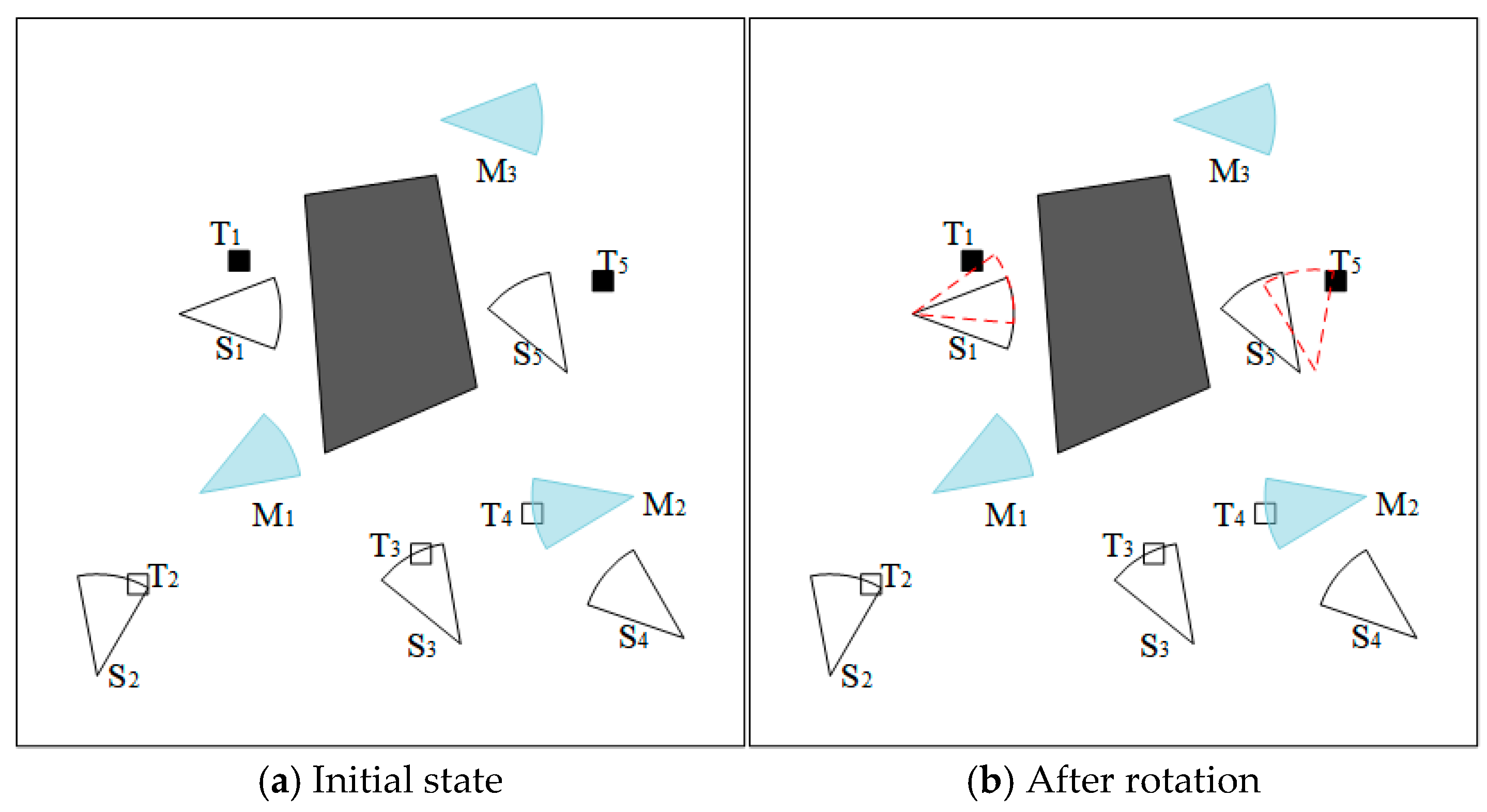
4.1.1. Repairing Coverage Hole Based on Adjusting Sensing Direction

There are many coverage holes in randomly deployed networks. For directed sensors, coverage gaps can be repaired by optimizing the working direction of nodes. Firstly, we determined the location of the coverage hole through the positioning device embedded in the sensor. Then, we calculated the length of the gap between the stationary sensor and the coverage hole. Finally, we broadcast notifications to stationary sensors that met the requirements for rotation. Stationary sensors that completed rotation will no longer participate in the next round of optimization.

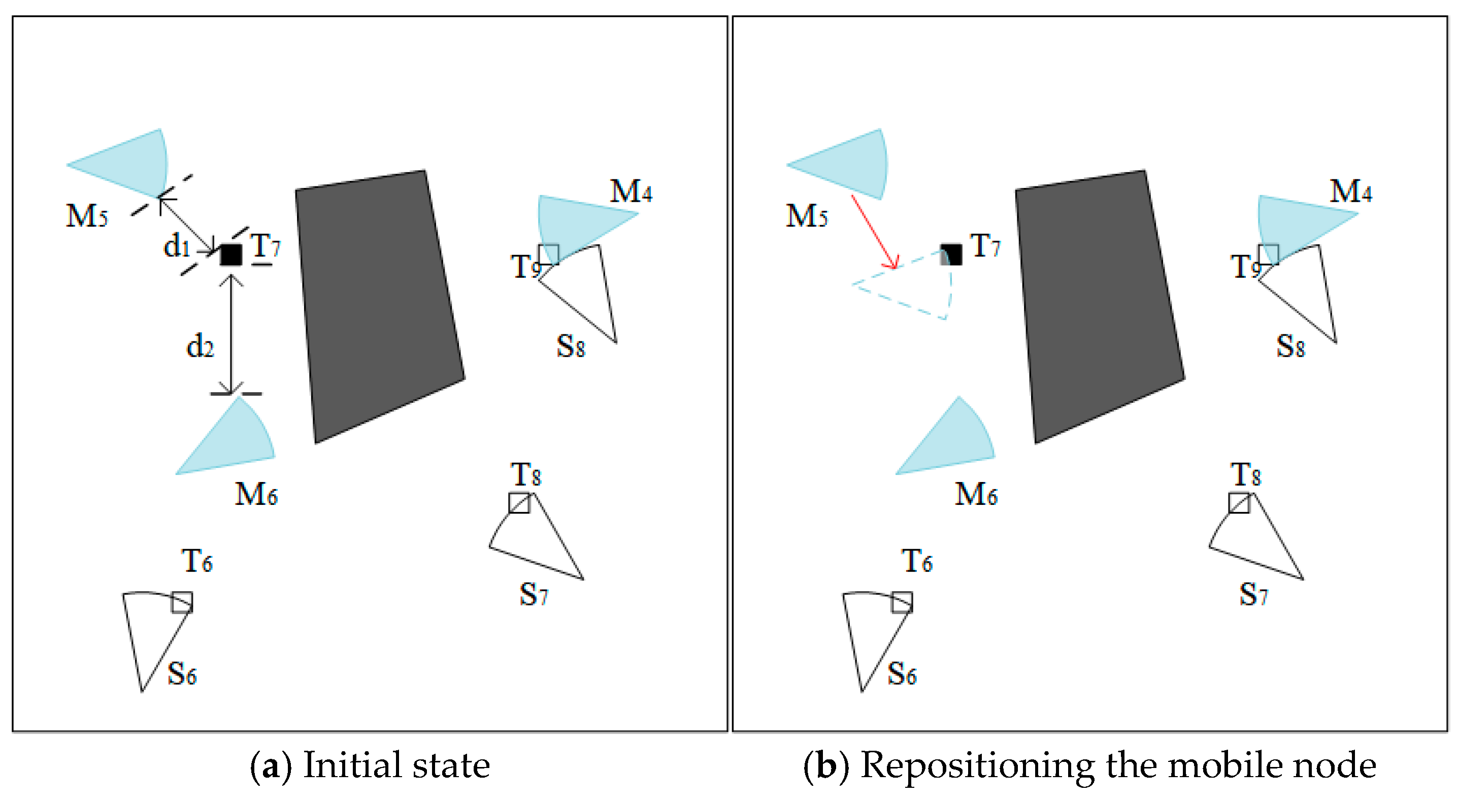
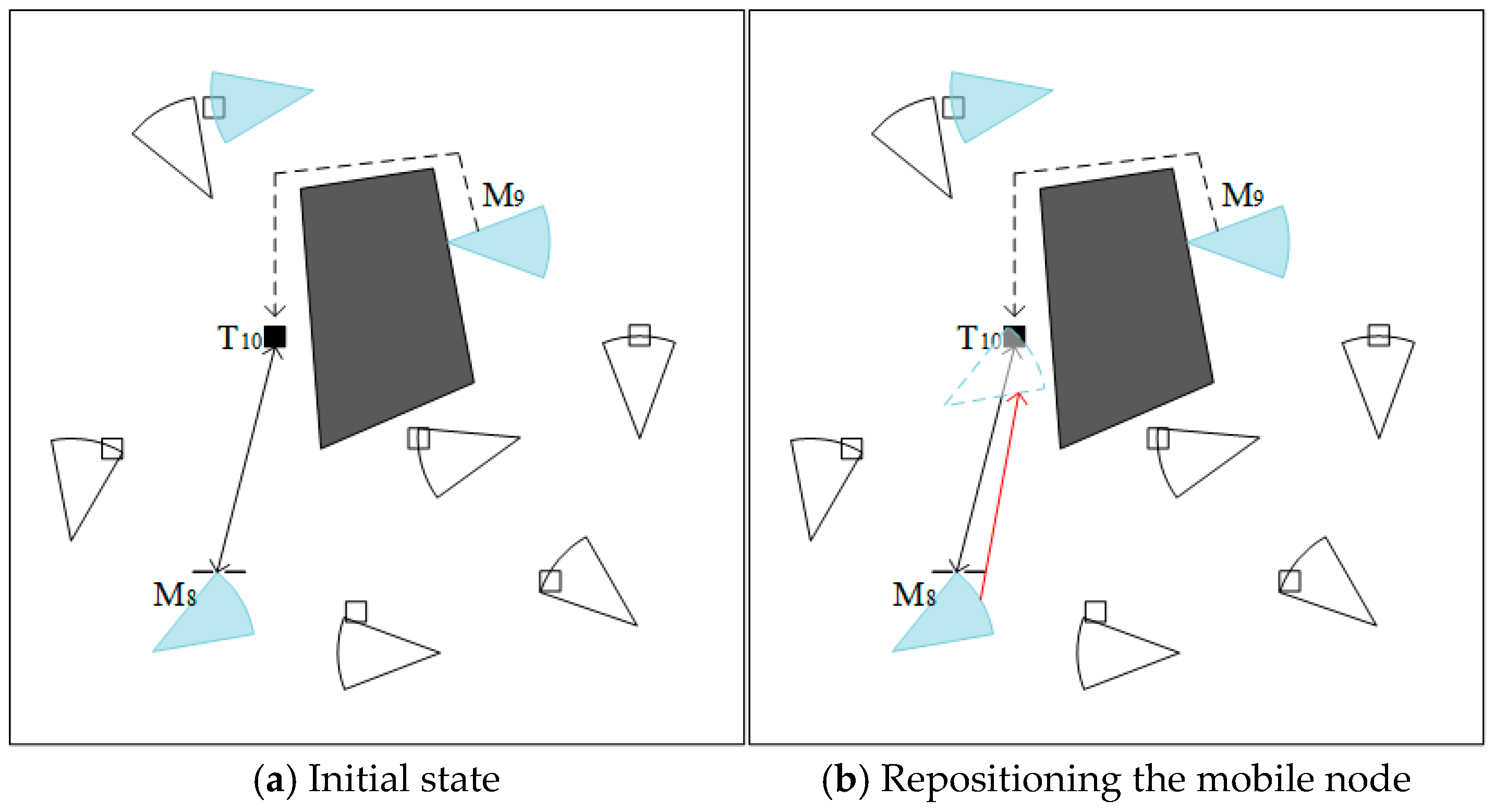
4.1.2. Obstacle Avoidance Path Planning Based on IBS-A* Algorithm

Obstacles in the monitoring area can hinder the scheduling of mobile sensors. Therefore, after determining the candidate nodes, we needed to design obstacle avoidance movement paths to schedule the nodes. The A* algorithm is a classic path planning method with good performance in calculating global optimized paths. The traditional A* algorithm suffers from problems such as multiple traversal nodes, large corners, and uneven paths. Moreover, traditional A* algorithms heavily rely on heuristic functions. To improve search speed and accuracy, we made improvements to the A* algorithm. Firstly, based on environmental information, we introduced obstacle probability factors and dynamically changed weight values to improve search accuracy. Then, a bidirectional search strategy was adopted to improve search speed. Finally, combined with the Floyd algorithm, unnecessary inflection points were removed, and the planned path was smoothly optimized.
(1)
Adaptive heuristic function
The heuristic function plays a key role in the search speed and accuracy of traditional A* algorithms. Our improvement of the heuristic function was divided into two parts. Firstly, we used 8-neighborhood search and combined the advantages of Euclidean distance and Manhattan distance to design the heuristic function. This heuristic function was closer to the actual cost. The improved heuristic function is shown below.
h ( n ) = d i s t x ( n ) + d i s t y ( n ) 0.2 × min d i s t x ( n ) , d i s t y ( n )
Then, we considered the influence of obstacles in the environment and introduced the obstacle probability factor. By changing the weight of the heuristic function h n , the evaluation function f n was adaptively adjusted.
f ( n ) = g ( n ) + 1 ln W h ( n )
W = N O D x n D y n
where N 0 represents the number of obstacles on the path, D x n = t x c x , D y n = t y c y . c x ,   t x represent the horizontal coordinates of the current point and the target point, respectively. c y ,   t y represent the vertical coordinates of the current point and the target point, respectively.
The weight of h n is negatively correlated with the number of obstacles. When the value of N 0 is large, the weight of h n actually decreases; on the contrary, the weight of h n increases. When the weight of h n is small, the accuracy of the algorithm can be ensured. Increasing the weight of h n can improve search speed.
(2)
Bidirectional search
The bidirectional A* algorithm performed 8-neighborhood search from both the starting point and the target point simultaneously. When two paths meet at a certain node, that path is the desired path. Moreover, to avoid the problem of intersecting paths with obstacles during bidirectional search, we added local path constraint search in the search strategy. Initialize two open lists and two closed lists, and add the starting point and target point to the open list for forward search and the open list for reverse search, respectively. Perform forward search and reverse search separately. When there was a common node in the open list of forward and reverse searches, the path was found. If the list was empty, it meant there was no path.
(3)
Path smoothing strategy
The path obtained through bidirectional search still has the problems of unsmooth path and large turning points. Therefore, it is necessary to remove redundant points in the path and perform smoothing processing. Firstly, starting from the second node, determine whether it is a redundant node. If the current node is on the same straight line as the previous node and does not pass through obstacles, then the node is a redundant node. Then, delete the redundant node and update the path. Finally, the Floyd algorithm was used to smooth the path and further optimize the planned path.

4.2. Extending Network Lifetime Based on Improved Nutcracker Optimizer Algorithm

After the coverage enhancement in phase 1, all targets were covered. However, there was still a problem of redundant coverage in the network. At time t, only one sensor needs to be activated at each target to complete the monitoring task. Simultaneously activating all sensors resulted in severe coverage redundancy, thereby reducing network lifetime. Therefore, when performing monitoring tasks, only some nodes are required to be turned on, while others enter sleep mode. We used INOA to solve this problem and obtain the optimal subset.

4.2.1. Nutcracker Optimizer Algorithm

The nutcracker optimizer algorithm (NOA) was proposed by Mohamed Abdel Basset et al. in 2023 [27,28]. Its principle is to simulate the behavior of nutcracker collecting and searching for food. The main framework of NOA consists of two strategies, each containing two population behaviors. There are two types of population behaviors included in these two strategies: exploration and exploitation.
A.
Foraging and storage strategy
The strategy consists of two main stages: foraging and storage. Each stage corresponds to a population behavior. The specific process is as follows.
(1)
Foraging stage: exploration phase 1
During the foraging and exploration phase, the initial position of the nutcracker is random. Firstly, the nutcracker checks the pine tree seeds at their initial position. If the seed quality at the initial position is good, the nutcracker flies back to the storage area from that position, and this path is a solution. Otherwise, the nutcracker will go to another location to search for good pine tree seeds. The position of the nutcracker was updated during this process. This process can be represented by the following mathematical equation.
X i t + 1 = X i , j t , i f τ 1 < τ 2 X m , j t + γ · X A , j t X B , j t + μ · U j L j , i f t T max / 2.0 X C , j t + μ · X A , j t X B , j t + μ · r 2 · U j L j , o t h e r w i s e o t h e r w i s e
where X i t + 1 represents the position of the nutcracker at the current iteration, and X i , j t represents the j-th position of the nutcracker at t iterations. τ 1 ,   τ 2 ,   r is a random real number within the range of [0, 1]. X m , j t represents the j-th dimensional mean of all solutions in the t-th iteration. γ ,   μ is a random real number between Levy flight and [0, 1] based on a normal distribution. A, B, and C are three random indices in the population. U j ,   L j are the upper and lower bounds of the j-dimensional variable. T max is the maximum number of iterations.
μ = τ 3 , r 1 < r 2 τ 4 , r 2 < r 3 τ 5 , r 1 < r 3
where r 1 ,   r 2 ,   r 3 are the random real numbers in the range [0, 1], τ 3 ,   τ 4 ,   τ 5 are random real numbers in the range [0, 1], normal distribution, and levy flight, respectively.
(2)
Storage stage: exploitation phase 1
During the development phase, the task of the nutcracker is to store food. The mathematical model of this behavior is shown below.
X i t + 1 n e w = X i t + μ · X b e s t t X i t · λ + r 1 · X A t X B t , τ 1 < τ 2 X b e s t t + μ · X A t X B t , τ 1 < τ 3 X b e s t t · l , o t h e r w i s e
where X i t + 1 n e w represents a new location in the storage area during t iterations, X b e s t t represents the current optimal solution, and λ is a random number. The linear decrease of l from 1 to 0 is an important factor in NOA. Its function is to avoid getting stuck in local minima and also to accelerate the convergence speed during the development phase.
To ensure a balance between explorers and developers during the foraging and storage stages, two random numbers φ and P a 1 were introduced. If φ > P a 1 , X i t + 1 = E q u a t i o n   20 . Otherwise, X i t + 1 = E q u a t i o n   22 . φ ,   P a 1 0 ,   1 . P a 1 decreases linearly with the number of iterations.
B.
Cache-search and recovery strategy
There are two behaviors in the search for storage areas and retrieval stages of the nutcracker population. The exploration and exploitation activities during this stage are as follows:
(1)
Cache-search stage: exploration phase 2
The search for storage areas and retrieval strategies are based on two reference points (RPs). Nutcracker chose two reference points to determine the location of the storage area. Nutcrackers have two methods when searching for storage areas: remembering R P 1 and remembering R P 2 . There are two possibilities for each method: the presence of food and the absence of food, as shown below.
X i , j t + 1 = X i , j t τ 3 < τ 4 X i , j t + r 1 X b e s t , j t X i , j t + r 2 R P i , 1 i X C , j t , τ 3 τ 4
X i , j t + 1 = X i , j t , τ 5 < τ 6 X i , j t + r 1 X b e s t , j t X i , j t + r 2 R P i , 2 i X C , j t , τ 5 τ 6
The first scenario of Equations (23) and (24) indicates the presence of food in the storage area, and the obtained solution is good and close to the optimal solution. In the next iteration, nutcracker may also choose this storage area. The second scenario indicates that there is no food in the area, and a new area needs to be searched. The choice of the first or second reference point for nutcracker is determined by τ 7 ,   τ 8 , τ 7 ,   τ 8 0 ,   1 .
X i t + 1 = E q u a t i o n   23 , τ 7 < τ 8 E q u a t i o n   24 , τ 7 τ 8
(2)
Recovery stage: exploitation phase 2
The basic principle of the retrieval phase is similar to the search for storage area phase, which is also implemented through two reference points. The location update equation for this phase is shown below.
X i t + 1 = X i t , f X i t < f R P i , 1 R P i , 1 , f X i t f R P i , 1
X i t + 1 = X i t , f X i t < f R P i , 2 R P i , 2 , f X i t f R P i , 2
Determine which reference point to choose by comparing f R P i , 1 ,   f R P i , 2 . If f R P i , 1 < f R P i , 2 , X i t + 1 = E q u a t i o n   26 . Otherwise, X i t + 1 = E q u a t i o n   27 .
X i t + 1 = E q u a t i o n   26 , f R P i , 1 < f R P i , 2 E q u a t i o n   27 , f R P i , 1 f R P i , 2
In order to ensure a balance between explorers and developers in the search for storage areas and retrieval stages, the latest positions of the two stages are randomly exchanged, as shown below.
X i t + 1 = E q u a t i o n 25 , ϕ > P a 2 E q u a t i o n 28 , ϕ P a 2
where ϕ is a random number within the range of [0, 1]. The value of P a 2 is 0.2.
However, in the NOA, if the quality of the solution is better than that of the new solution, nutcracker will remain at its current position.
X i t + 1 = X i t + 1 , i f f X i t + 1 > f X i t X i t , o t h e r w i s e

4.2.2. Improvement of Nutcracker Optimizer Algorithm

NOA is a recently proposed optimization algorithm that has the advantages of simple parameters and strong optimization ability [29]. However, NOA also has certain limitations, such as local optima and convergence problems. To further improve the performance of NOA, we introduced three strategies, as shown below.
(1)
Bidirectional local search
The bidirectional search strategy is to start searching from both the starting and ending points simultaneously, selecting a node from each direction to expand until the two search paths meet. During the search process, if there is a common point in the open list of forward and reverse searches, then that point is the optimal solution. If there are multiple different solutions, compare the fitness values of the solutions from multiple dimensions. Adding bidirectional search to the NOA can reduce the search space. Because it searches from both directions simultaneously, it can find solutions faster. Therefore, to further accelerate the search speed of NOA, this section adopts a bidirectional search strategy.
(2)
Cauchy mutation operation
The Cauchy mutation operation updates the position of an individual. The offspring produced by it have greater differences from their parents. Therefore, the diversity of the population was increased, and the global optimization ability of the algorithm was improved. There are three main steps to implementing Cauchy mutation operation: (1) After the algorithm enters a premature state, sort the current fitness values of individuals in ascending order. (2) Perform Cauchy perturbation on the positions of the top 15% individuals and maintain them within the solution space to prevent them from crossing boundaries. (3) Recalculate the fitness size of the individual and determine whether it has fallen into premature convergence. If so, repeat steps (1) to (3) until the global optimal value is searched or the algorithm termination condition is met.
(3)
Fusion improvement strategy
To improve the convergence speed of NOA while reducing local minima, we designed a fusion improvement strategy. Firstly, choose a random solution. Then, compare the fitness values of the random solution with the current solution. If the fitness value of the current solution is high, update along the direction of the current solution until the optimal solution is found. Otherwise, update the current solution in the direction of the random solution. This strategy reduces the probability of excellent solutions being eliminated by introducing random schemes, increases the diversity of solutions, and reduces the possibility of local optima. Meanwhile, as the search direction is concentrated in areas with high fitness values, the convergence speed is faster.
Algorithm 1 shows the improved NOA.
Algorithm 1 Improved Nutcracker Optimization Algorithm (INOA)
Input:   P ,   U ,   L ,   T max
Output:   the   best   solution   found   X b e s t
1: Initialize the population
2: Find the current solution with the highest fitness value
3:    t = 1
4:    while  t < T max
5:       Generate   random   real   numbers   β ,   β 1 from [0, 1]
6:     if   β < β 1 //Foraging and storage strategy//
7:       φ ,   P a 1 are random number within [0, 1]
8:      for i = 1:N
9:        for j = 1:d
10:       if   φ > P a 1
11:          update   X i t + 1 using Equations (20) and (30)
12:          else
13:               update   X i t + 1 using Equations (22) and (30)
14:            end if
15:            t = t + 1
16:          end for
17:      else     //Cache-search and recovery strategy//
18:        Generate RP, and random numbers ϕ within [0, 1]
19:          for i = 1:N
20:            if   ϕ > P a 2
21:             update   X i t + 1 using Equations (25) and (30)
22:              else
23:           update   X i t + 1 using Equations (28) and (30)
24:          end if
25:    t = t + 1
26: end for
27: else     //Improvement strategy//
28:     for i = 1:N
29: Calculate the fitness values of solutions under different improvement strategies
30:        Compare fitness values
31:         update   X i t + 1
32:      end if
33:        t = t + 1
34:      end for
35:  end while

5. Simulation Result

We conducted multiple experiments in this section, and we analyzed and summarized the experimental results. We evaluated the capability of our method through a result analysis. Considering the error of a single experiment, all experimental data are the average of multiple experiments. The experiments in this paper were conducted on MATLAB 2018a, and the experimental platform used was a Windows 10 system.
As described in Section 4, our method consists of three parts: optimizing the sensing direction of stationary nodes, updating the deployment location of mobile nodes, and scheduling node sleep or work. Among them, optimizing node sensing directions and updating node positions are aimed at covering uncovered targets and improving coverage capability. The purpose of arranging sensors to sleep or work is to increase the remaining energy and improve monitoring time. We designed two sets of experiments in this section to evaluate the reliability and superiority of our method.
The purpose of Experiment A is to evaluate the ability of our method in coverage enhancement by comparing the uncovered targets and their moving distances. The amount of uncovered targets determines the quality of network monitoring, and the distance represents the energy consumed. They are the most important indicators for evaluating coverage enhancement methods. This paper adopts a stationary node sensing direction optimization method and a mobile node scheduling method based on IBS-A* to achieve coverage enhancement.
The A* algorithm is a classic path search algorithm widely used in coverage enhancement. The multi-objective particle swarm optimization (MOPSO) enhances network coverage by searching for the optimal location of mobile nodes. An improved vampire bat–virtual force algorithm (VB-IVFA) combines the improved virtual force and vampire bat algorithm to schedule nodes for enhanced coverage. Therefore, in Experiment A, we compared the proposed IBS-A* with the A* algorithm, MOPSO [24], and VB-IVFA [19] algorithms.
The purpose of Experiment B is to evaluate the ability of our method in extending the network lifetime. This paper uses the INOA to solve the optimal working timing of nodes, scheduling a subset of nodes to work alternately, thereby extending the network lifetime. The two-phase lifetime-enhancing method (TLM) [24], maximizing the surveillance quality of area coverage (MSQAC) [30], and the maximum coverage set scheduling algorithm (MCSSA) [31] all extend the network lifetime by solving node subsets. Therefore, we compared the proposed INOA with the TLM, MSQAC, and MCSSA. Specifically, we also compared the INOA with the original NOA. In addition, due to the fact that the TLM, MSQAC, and MCSSA use omnidirectional sensing models, they cannot be directly applied to directional sensing models. We have modified these three algorithms based on the method in reference [13] to enable their application in directional sensor networks.

5.1. Parameter Settings

In this experiment, the monitoring area is set to 200   m × 200   m , the number of sensors n is 50–500, and the number of targets k is 10–50. The sensing radius of the sensor R s is 10 m, and the communication radius is R c = 2 R s . The initial energy E of the sensor is 10 U, and the maximum capacity of the sensor is also 10 U. The energy threshold E th of the sensor is 0.6 E . The sensing energy consumption rate of the sensor e s sens d i s c h is 0.5 U/T. The energy consumption of mobile sensors e s m o v e d i s c h is 0.1 U/m. The charging rate of sensors e s c h a r is related to weather conditions. We refer to the method in reference [25] to predict the solar energy intensity for the day based on historical data, in order to determine the charging rate. The range of the charging rate is 0–0.5 U/T. The specific parameters are shown in Table 1.

5.2. Experiment A: Comparing of Coverage Enhancement Performance

We designed three experiments to verify the ability of the proposed IBS-A* algorithm in uncovered targets and movement distance. The three experiments are as follows: the visualization example, comparison of the obstacle avoidance path length for individual sensors, and comparison of the total obstacle avoidance path length (total movement distance). In addition, when comparing the total movement distance, we also compared uncovered targets to estimate the ability of the IBS-A* algorithm.

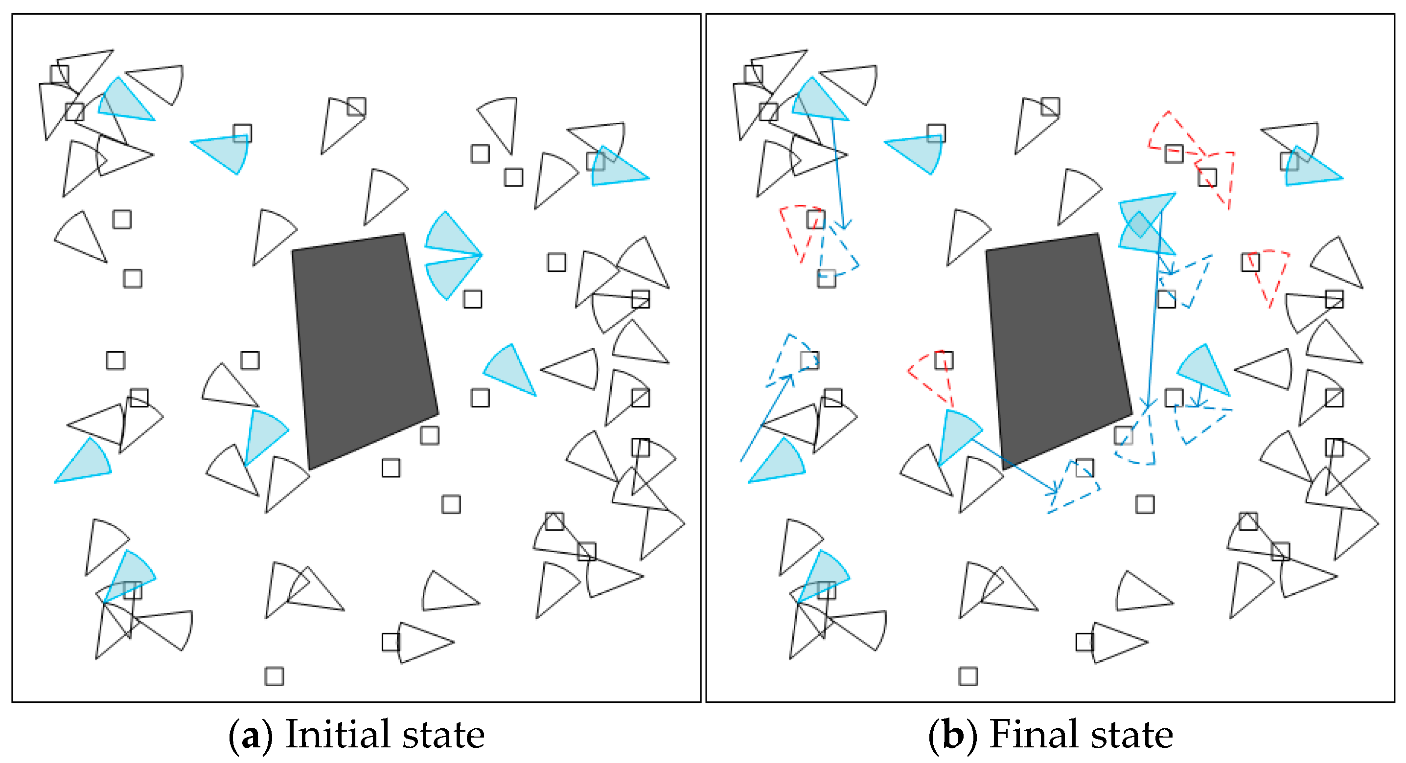
5.2.1. Visualization Example

Figure 7 shows a visualization example after executing the coverage enhancement algorithm. Figure 7a is a monitoring area where sensors are randomly deployed, and Figure 7b is the state after executing our algorithm. The white rectangle and sector are the target and stationary nodes, respectively. The blue sector is the mobile sensor node. The black polygon represents obstacles. The red dashed sector represents the new position of the static sensor after rotation. The blue dashed sector represents the new position of the mobile sensor. The blue arrow represents the movement path of the mobile sensor. From Figure 7a, it can be seen that there are 13 uncovered targets. After executing the algorithm, there are only two uncovered targets in the monitoring area. Therefore, implementing the method proposed in this paper can effectively repair coverage holes and enhance network coverage.

5.2.2. Comparison of Obstacle Avoidance Path Lengths for Individual Sensors

To compare the search accuracy and search time of IBS-A*, A*, MOPSO, and VB-IVFA, we conducted obstacle avoidance movement experiments using a single sensor. Table 2 lists the obstacle avoidance path length and search time of IBS-A* compared to three other algorithms.
From the table, the obstacle avoidance path of A* algorithm is smaller than MOPSO and the VB-IVFA. Compared to MOPSO and the VB-IVFA, the A* algorithm has better search performance. Our IBS-A* algorithm incorporates a smoothing strategy into the traditional A* algorithm, reducing unnecessary inflection points. Therefore, the IBS-A* algorithm searches for the optimal path that is 6.3% smaller than the A* algorithm. In addition, the IBS-A* algorithm introduces a bidirectional search method to improve search speed, resulting in a 53.1%, 61.7%, and 68.5% increase in search time compared to A*, MOPSO, and VB-IVFA, respectively.

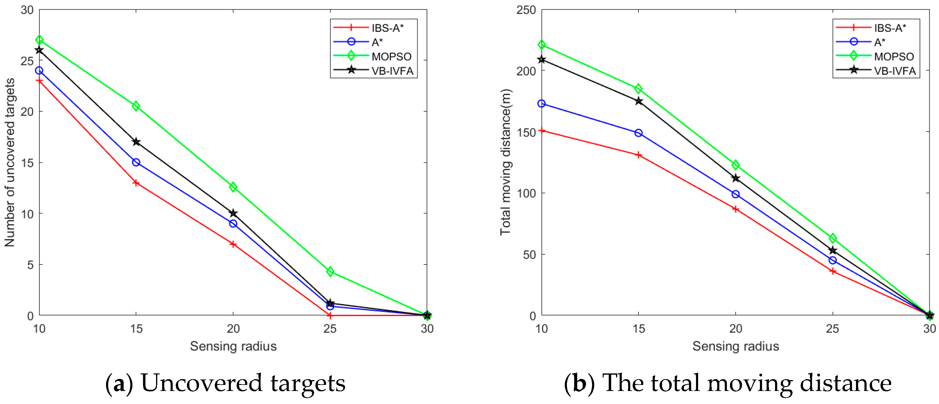
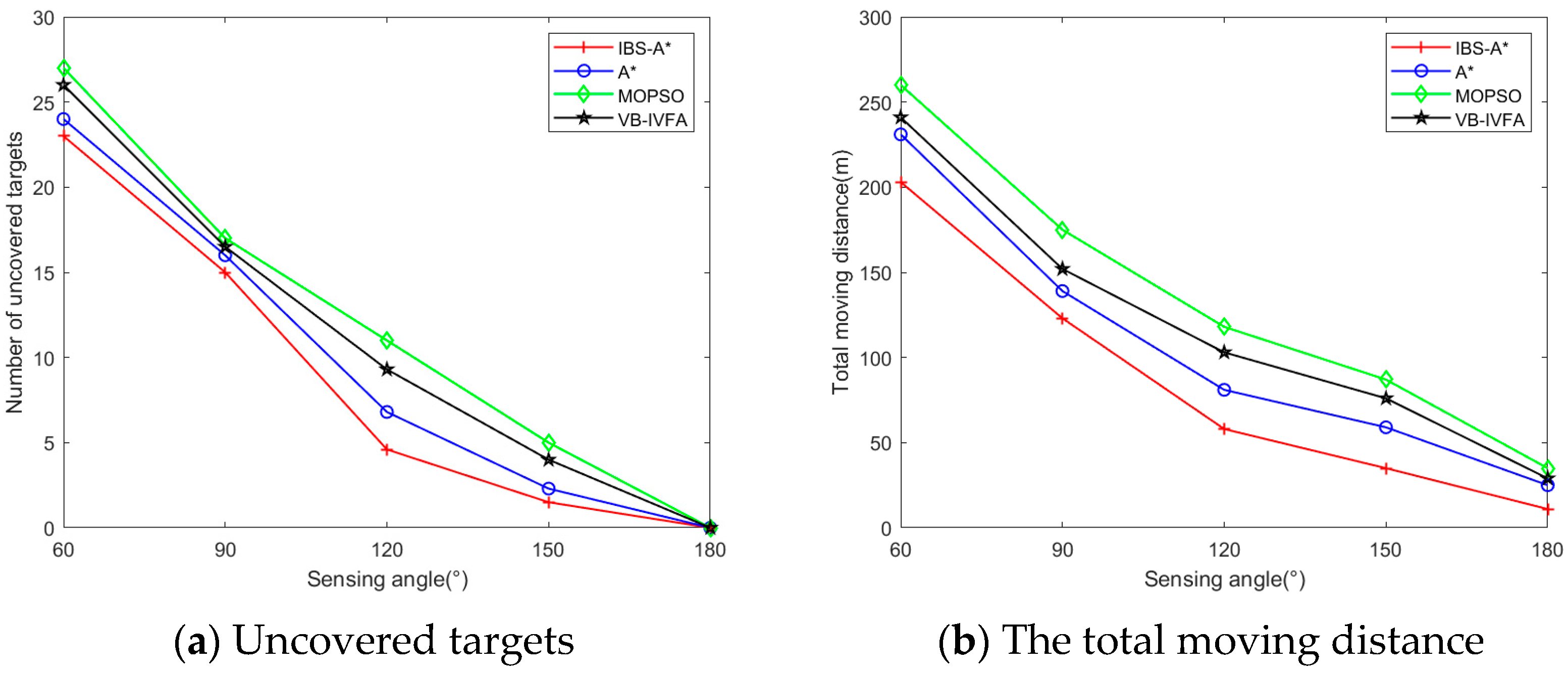
5.2.3. Comparison of Uncovered Targets and Total Moving Distance in Different Scenarios

In this section of the experiment, we performed IBS-A*, A*, MOPSO, and VB-IVFA separately, and we present the experimental results in the figure. The experimental parameters include the following: n , k , R s , θ . Among them, n is 100, and k is 50. We conducted experiments in environments with different proportions of mobile sensors, sensing radii R s , and sensing angles θ .
As shown in Figure 8, we compared the results of different methods in uncovered targets and mobile energy consumption under different proportions of mobile sensors. Mobile energy consumption mainly focuses on the energy consumed during movement. Therefore, the energy consumption of movement is represented by the distance traveled. In this experiment, R s and θ were set to 10 m, π / 2 , respectively.
From Figure 8, when the proportion of mobile sensors becomes larger, the uncovered targets show a decreasing trend, while the moving distance shows an increasing trend. As shown in Figure 8a, in terms of uncovered targets, the results of IBS-A* are very close to those of A*, MOPSO, and the VB-IVFA. When the proportion of mobile sensors reaches a certain value, all targets in the monitoring area are covered by the sensors. But, in Figure 8b, our algorithm has a significant advantage in terms of movement distance. The A*-based method can search for the most suitable path, but its performance is poor in obstacle environments. However, the obstacle avoidance paths planned by the MOPSO algorithm and the VB-IVFA have many turning points and are not smooth enough. Also, our method has good obstacle avoidance ability, and the path is relatively smooth. Therefore, the moving distance generated by the above three algorithms is higher than our method. With A*, MOPSO, and the VB-IVFA, the IBS-A* method reduces the total moving distance by 10.5%, 23.1%, and 18.3%, respectively.
Figure 9 and Figure 10, respectively, demonstrate the performance of four algorithms under different sensing radii and angles. As shown in Figure 9a and Figure 10a, in terms of uncovered targets, all algorithms exhibit a decreasing trend. When the perceived radius and angle increase to a certain extent, the performance of the four algorithms is very similar. In terms of moving distance, it is evident from the analysis of the experimental data in Figure 9b and Figure 10b that the proposed IBS-A* has the smallest moving distance, followed by the VB-IVFA, and MOPSO has the highest value. This indicates that the proposed method has less mobile energy consumption while meeting coverage requirements, which is more conducive to extending the network lifetime.
In summary, our IBS-A* algorithm has certain advantages in coverage rate, moving distance, running time, and other aspects. While meeting coverage requirements, it can also reduce mobile energy consumption, laying a foundation for extending network lifetime in the next step.

5.3. Experiment B: Comparison of Network Lifetime

We compared the performance of the proposed INOA with NOA, TLM, MSQAC, and MCSSA algorithms in network lifetimes. We implemented five algorithms in the case of different numbers of sensors n , sensing radius R s , sensing angle θ , and target k .

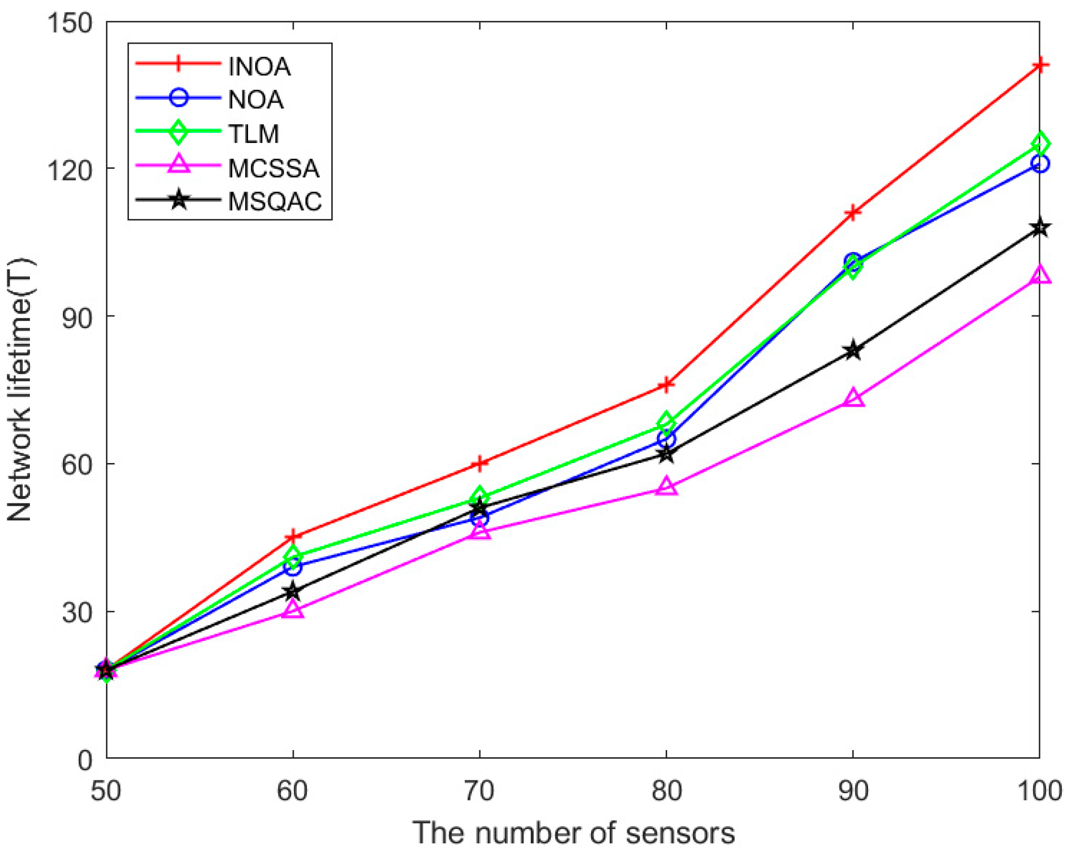
5.3.1. Comparing the Impact of Sensor Numbers on Network Lifetime

The network lifetime of five algorithms under different sensor numbers is shown in Figure 11. Experimental parameters: k , R s , and θ are set as 50, 10 m, and, respectively. The proportion of mobile sensors is 0.2, and n is 50–100. By analyzing the experimental data in Figure 11, it is evident that, as the number of sensors enhanced from 50 to 100, the network lifetime also continued to rise. More sensors mean that multiple sensors can be deployed at certain targets. Therefore, more work subsets that meet coverage requirements can be obtained. The more subsets that meet the criteria, the longer the network lifetime. Compared to the TLM, MSQAC, and MCSSA, the proposed INOA method has a longer network lifetime. Under the same conditions, compared with the TLM, MSQAC and MCSSA, the maximum improvement of the INOA is 12.8%, 30.6%, and 43.9%, respectively, and the average improvement is 5.9%, 15.8%, and 22.3%, respectively. Compared to the NOA, the INOA has a maximum increase of 16.3% and an average increase of 8.7%. Compared with the NOA, the INOA has added a Cauchy mutation operator and fusion improvement strategy, which enriches the diversity of the population and improves the global optimization ability of the algorithm. Therefore, the lifetime of the subset of nodes obtained by the INOA is longer.

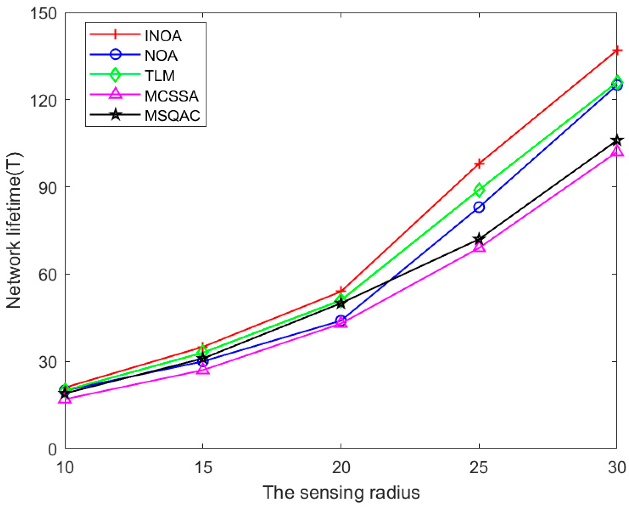
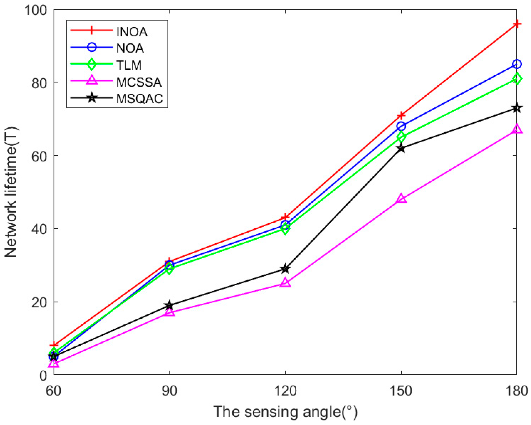
5.3.2. Comparing the Impact of Sensing Radii and Angles on Network Lifetime

The network lifetime of five algorithms under different sensing radii is shown in Figure 12. n , k , and θ are set as 50, 50, and, respectively. The proportion of mobile sensors is 0.2, and R s is 10–50 m. As shown in Figure 12, the network lifetime of all five algorithms shows an upward trend. The larger the value of the sensing radius, the larger the coverage range of the sensor node. Sensors with larger coverage areas can cover more targets. Therefore, fewer sensors are used to perform monitoring tasks, thereby extending the network lifetime. The sensing radius of the sensor reached beyond 20 m, showing that the improvement in network lifetime is more significant. With the NOA, compared to the TLM, MSQAC, and MCSSA, the INOA has always had the best network lifetime.
The network lifetime of five algorithms under different sensing angles is shown in Figure 13. n , k and R s are set as 50, 50, and 10 m, respectively. The proportion of mobile sensors is 0.2, and θ is π / 3 ,   π . Similar to the experimental results under different sensing radii, the network lifetime is positively correlated with the sensing angles of sensor nodes.

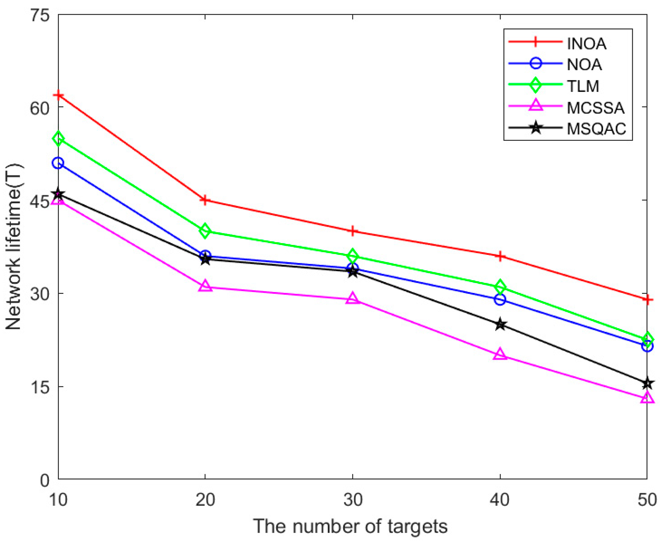
5.3.3. Comparing the Impact of Target Numbers on Network Lifetime

The network lifetime of five algorithms under different numbers of targets is shown in Figure 14. n , R s , and θ are set as 100, 10 m, and, respectively. The proportion of mobile sensors is 0.2, and the number of targets is 10–50. The increase in targets means that more sensors need to be scheduled to perform monitoring tasks, which requires more energy consumption. The lifetime of the network is negatively correlated with target numbers. From the experimental data in the figure, it can be seen that, when the number of targets is the same, the INOA has the longest network lifetime. Compared to the NOA, TLM, MSQAC, and MCSSA, the average improvement of the INOA proposed is 14.7%, 13.6%, 45.3%, and 56.1%, respectively.
As mentioned above, in four different cases, the proposed INOA outperforms the NOA, TLM, MSQAC, and MCSSA in network lifetimes. Therefore, the method proposed in this paper is effective and has good performance.

6. Conclusions

This paper proposes a new node deployment optimization method to solve the problems of coverage quality and network lifetime in obstacle environments. This method repairs coverage holes and enhances network coverage by solving for the optimal sensing direction of stationary sensors and designing a shortest obstacle avoidance path for mobile sensors. After enhancing network coverage, this paper proposes a sensor working state (work sleep) adjustment method based on the INOA. This method arranges subsets of nodes in order to perform coverage tasks, thereby extending the network lifetime. From experimental data and analysis, it can be seen that, compared with A*, MOPSO, and the VB-IVFA, the IBS-A* method proposed in this paper reduces the average moving distance by 10.5–23.1%. In terms of network lifetime, compared with the NOA, TLM, MSQAC, and MCSSA, the average improvement of the INOA is 5.9–22.3%. The maximum improvement rate reached 56.1%. Therefore, the proposed method has better performance, can improve the coverage rate with a smaller moving distance, and effectively prolong the network lifetime. However, the work presented in this paper can be further expanded. We may consider using distance-adjustable sensors or probabilistic sensing models in our future research. In addition, introducing UAVs to assist in replenishing energy is another potential research work.

Author Contributions

Conceptualization, P.W. and Y.X.; methodology, P.W. and Y.X.; software, P.W.; validation, P.W. and Y.X.; formal analysis, P.W.; investigation, P.W.; resources, P.W.; data curation, Y.X.; writing—original draft preparation, P.W.; writing—review and editing, P.W. and Y.X.; visualization, P.W.; supervision, Y.X.; project administration, Y.X.; funding acquisition, Y.X. All authors have read and agreed to the published version of the manuscript.

Funding

This research was funded by the National Natural Science Foundation of China (61873249).

Institutional Review Board Statement

Not applicable.

Informed Consent Statement

Not applicable.

Data Availability Statement

The raw data supporting the conclusions of this article will be made available by the authors upon request.

Conflicts of Interest

The authors declare no conflicts of interest.

References

  1. Liang, J.B.; Tu, J.K.; Leung, V.C.M. Mobile sensor deployment optimization algorithm for maximizing monitoring capacity of large-scale acyclic directed pipeline networks in smart cities. IEEE Internet Thing J. 2021, 8, 16083–16095. [Google Scholar] [CrossRef]
  2. Deng, C.; Fu, X.W. Low-AoI data collection in UAV-aided wireless-powered IoT based on aerial collaborative relay. IEEE Sens. J. 2024, 20, 33506–33521. [Google Scholar] [CrossRef]
  3. Nguyen, T.T.; Pan, J.S.; Dao, T.K. A novel improved Bat algorithm based on hybrid parallel and compact for balancing an energy consumption problem. Information 2019, 10, 194. [Google Scholar] [CrossRef]
  4. Nkemeni, V.; Mieyeille, F.; Tsafack, P. Energy consumption reduction in wireless sensor network-based water pipeline monitoring systems via energy conservation techniques. Future Internet 2023, 15, 402. [Google Scholar] [CrossRef]
  5. Zhang, C.; Li, Y.X.; Xu, P. Dynamic probabilistic sensing for enhanced target coverage in WRSNs. IEEE Sens. J. 2024, 24, 26699–26715. [Google Scholar] [CrossRef]
  6. Yao, Y.D.; Yang, Y.; Tian, Y.Y. Improved genetic algorithm-based MEP search strategy for DSNs intrusion detection. IEEE Sens. J. 2024, 24, 33544–33559. [Google Scholar] [CrossRef]
  7. Xu, C.J.; Su, S.C.; Wang, Y.W. An improved stochastic fractal search based on entropy multitrust fusion model for IoT-enabled WSNs clustering. IEEE Sens. J. 2023, 23, 29694–29704. [Google Scholar] [CrossRef]
  8. Chen, Y.; Zhao, Y.B.; Ge, Y.M. Game-theoretic power allocation scheme of cooperative localization in hybrid active–passive wireless sensor networks. IEEE Internet Thing J. 2024, 11, 33027–33039. [Google Scholar] [CrossRef]
  9. Mishra, A.M.; Agrawal, K.; Prakriya, S. Performance of a cluster-based multihop IoT network with battery-assisted energy harvesting. IEEE Internet Thing J. 2025, 12, 5901–5917. [Google Scholar] [CrossRef]
  10. Gonzalez, P.; Mujica, G.; Portilla, J. The application of evolutionary, swarm, and iterative-based task-offloading optimization for battery life extension in wireless sensor networks. IEEE Sens. J. 2024, 24, 26682–26698. [Google Scholar] [CrossRef]
  11. Cho, H.H.; Chien, W.C.; Tseng, F.H.; Chao, H.C. Artificial-intelligence-based charger deployment in wireless rechargeable sensor networks. Future Internet 2023, 15, 117. [Google Scholar] [CrossRef]
  12. Chen, Y.; Deng, T.D.; Tang, S.Q. A charging scheme for large-scale suburban WRSNs based on the collaboration of UAVs and mobile PADs. IEEE Sens. J. 2025, 25, 5615–5629. [Google Scholar] [CrossRef]
  13. Wang, P.; Xiong, Y.H. A method to optimize deployment of directional sensors for coverage enhancement in the sensing layer of IoT. Future Internet 2024, 16, 302. [Google Scholar] [CrossRef]
  14. Wang, P.; Xiong, Y.H.; She, J.H. A new closed-barrier covering optimization method for heterogeneous nodes in hybrid wireless sensor networks. In Proceedings of the 47th Annual Conference of the IEEE Industrial Electronics Society, Toronto, ON, Canada, 13–16 October 2021. [Google Scholar]
  15. Yao, Y.D.; Wen, Q.; Cui, Y.P.; Zhao, B.Z. Discrete army ant search optimizer-based target coverage enhancement in directional sensor networks. IEEE Sens. Lett. 2022, 6, 1–4. [Google Scholar] [CrossRef]
  16. Liu, S.; Zhang, R.L.; Shi, Y.H. Design of coverage algorithm for mobile sensor networks based on virtual molecular force. Comput. Commu. 2020, 15, 269–277. [Google Scholar] [CrossRef]
  17. Chen, G.; Xiong, Y.H.; She, J.H. A k-barrier coverage enhancing scheme based on gaps repairing in visual sensor network. IEEE Sens. J. 2023, 23, 2865–2877. [Google Scholar] [CrossRef]
  18. Yao, Y.D.; Li, Y.; Xie, D.Y. Coverage enhancement strategy for WSNs based on virtual force-directed ant lion optimization algorithm. IEEE Sens. J. 2021, 21, 19611–19622. [Google Scholar] [CrossRef]
  19. Wen, Q.; Zhao, X.Q.; Cui, Y.P.; Zeng, Y.P. Coverage enhancement algorithm for WSNs based on vampire bat and improved virtual force. IEEE Sens. J. 2022, 22, 8245–8256. [Google Scholar] [CrossRef]
  20. Peng, S.; Xiong, Y.H. A lifetime-enhancing method for directional sensor networks with a new hybrid energy-consumption pattern in Q-coverage scenarios. Energies 2020, 13, 824. [Google Scholar] [CrossRef]
  21. Tarip, U.U.; Ali, H.; Hussain, M. Shuffled ARSH-FATI: A novel meta-heuristic for lifetime maximization of range-adjustable wireless sensor networks. IEEE Trans. Green. Commun. Netw. 2023, 7, 1217–1233. [Google Scholar]
  22. Chen, Z.G.; Lin, Y.; Gong, Y.J. Maximizing lifetime of range-adjustable wireless sensor networks: A neighborhood-based estimation of distribution algorithm. IEEE Intern. Trans. Cyber. 2021, 51, 5433–5444. [Google Scholar] [CrossRef] [PubMed]
  23. Liu, J.X.; Jian, P.; Xu, W.Z. Maximizing sensor lifetime via multi-node partial-charging on sensors. IEEE Trans. Mobile. Comput. J. 2023, 22, 6571–6584. [Google Scholar] [CrossRef]
  24. Xiong, Y.H.; Chen, G.; Lu, M.J. A two-phase lifetime-enhancing method for hybrid energy-harvesting wireless sensor network. IEEE Sens. J. 2020, 20, 1934–1946. [Google Scholar] [CrossRef]
  25. Xu, P.; Wang, X.F.; Chang, C.Y. JMLA: Joint monitoring quality and network lifetime for range-adjustable sensors in WRSNs. IEEE Sens. J. 2024, 24, 33522–33543. [Google Scholar] [CrossRef]
  26. Xiong, D.; Liu, Y.F.; Zhu, C.; Jin, L.; Wang, L.M. Delay-dependent stability analysis of haptic systems via an auxiliary function-based integral inequality. Actuators 2021, 10, 171. [Google Scholar] [CrossRef]
  27. Basset, M.A.; Mohamed, R.; Jameel, M. Nutcracker optimizer: A novel nature-inspired metaheuristic algorithm for global optimization and engineering design problems. Knowl. System. 2023, 262, 110248. [Google Scholar] [CrossRef]
  28. Evangeline, S.I.; Darwin, S.; Anandkumar, P.P. Investigating the performance of a surrogate-assisted nutcracker optimization algorithm on multi-objective optimization problems. Expert. System. Appli. 2024, 245, 123044. [Google Scholar] [CrossRef]
  29. Mahamed, A.B.; Reda, M.; Ibrahim, M.H. An improved nutcracker optimization algorithm for discrete and continuous optimization problems: Design, comprehensive analysis, and engineering applications. Heliyon 2024, 10, e36678. [Google Scholar]
  30. Dande, B.; Chang, C.Y.; Liao, W.H. MSQAC: Maximizing the surveillance quality of area coverage in wireless sensor networks. IEEE Sens. J. 2022, 22, 6150–6163. [Google Scholar] [CrossRef]
  31. Luo, C.W.; Hong, Y.; Li, D.Y. Maximizing network lifetime using coverage sets scheduling in wireless sensor networks. Ad. Hoc. Netw. 2020, 98, 102037. [Google Scholar] [CrossRef]
Figure 1. Directional sensing model.
Information 16 00228 g001
Figure 2. Adjust the sensing direction of stationary nodes.
Information 16 00228 g002
Figure 3. Scheduling mobile nodes to repair coverage holes: case 1.
Information 16 00228 g003
Figure 4. Scheduling mobile nodes to repair coverage holes: case 2.
Information 16 00228 g004
Figure 5. The process of scheduling nodes to extend the network lifetime.
Information 16 00228 g005
Figure 6. Basic framework of the proposed method.
Information 16 00228 g006
Figure 7. Visualization of performing proposed method.
Information 16 00228 g007
Figure 8. Uncovered targets and total moving distance with various ratios of mobile sensors.
Information 16 00228 g008
Figure 9. Uncovered targets and total moving distance with various sensing radius.
Information 16 00228 g009
Figure 10. Uncovered targets and total moving distance with various sensing angles.
Information 16 00228 g010
Figure 11. Network lifetime under various sensor numbers.
Information 16 00228 g011
Figure 12. Network lifetime under various sensing radius.
Information 16 00228 g012
Figure 13. Network lifetime under various sensing angles.
Information 16 00228 g013
Figure 14. Network lifetime under various target numbers.
Information 16 00228 g014
Table 1. Simulation parameters.
Region of Interest (ROI)200 m × 200 m
Number of targets (k) 10 ,   50
Number of sensors (n) 50 ,   500
Number of stationary sensors ( n s ) 0 ,   500
Number of mobile sensors ( n m ) 0 ,   500
Sensing angles ( θ ) π / 3 ,   π
Sensing radius ( R s )10 m
Communication radius ( R c )20 m
Initial energy ( E )10 U
Energy threshold ( E t h )0.6 E
Sensing energy consumption ( e s sens d i s c h )0.5 U/T
Mobile energy consumption ( e s m o v e d i s c h )0.1 U/m
Charging rate ( e s c h a r )0–0.5 U/T
Table 2. The path length and search time of different algorithms.
The Length of Obstacle Avoidance Path (m)Search Time (s)
A*39.757.81
MOPSO46.629.53
VB-IVFA45.3311.56
IBS-A*37.253.65
Disclaimer/Publisher’s Note: The statements, opinions and data contained in all publications are solely those of the individual author(s) and contributor(s) and not of MDPI and/or the editor(s). MDPI and/or the editor(s) disclaim responsibility for any injury to people or property resulting from any ideas, methods, instructions or products referred to in the content.

