


An Expected Value-Based Symmetric–Asymmetric Polygonal Fuzzy Z-MCDM Framework for Sustainable–Smart Supplier Evaluation


Abstract

1. Introduction
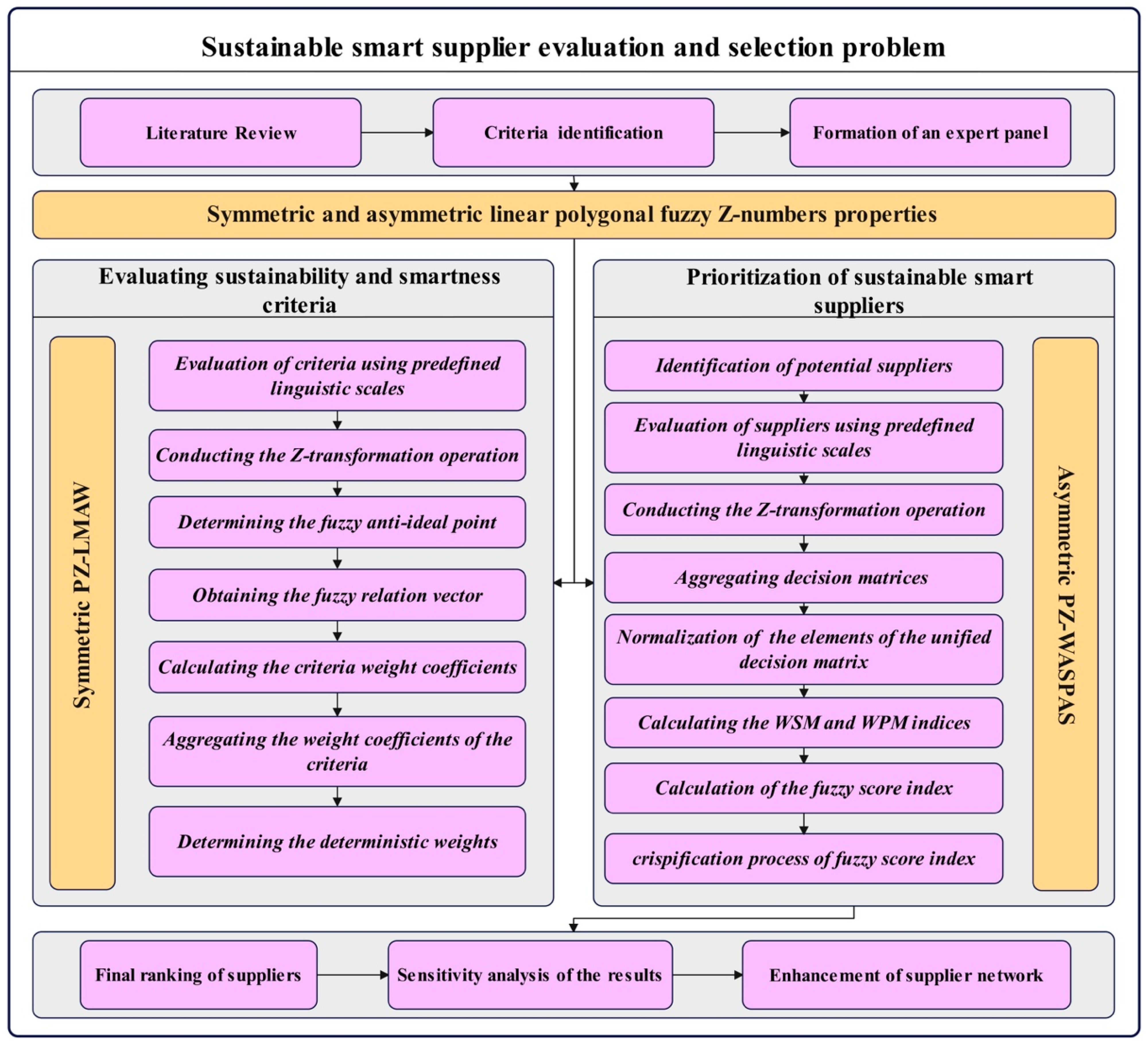
- Conducting a literature review and identifying the factors and criteria influencing the process of sustainable smart SES, complemented by a real-world case study in the home appliance supply chain.
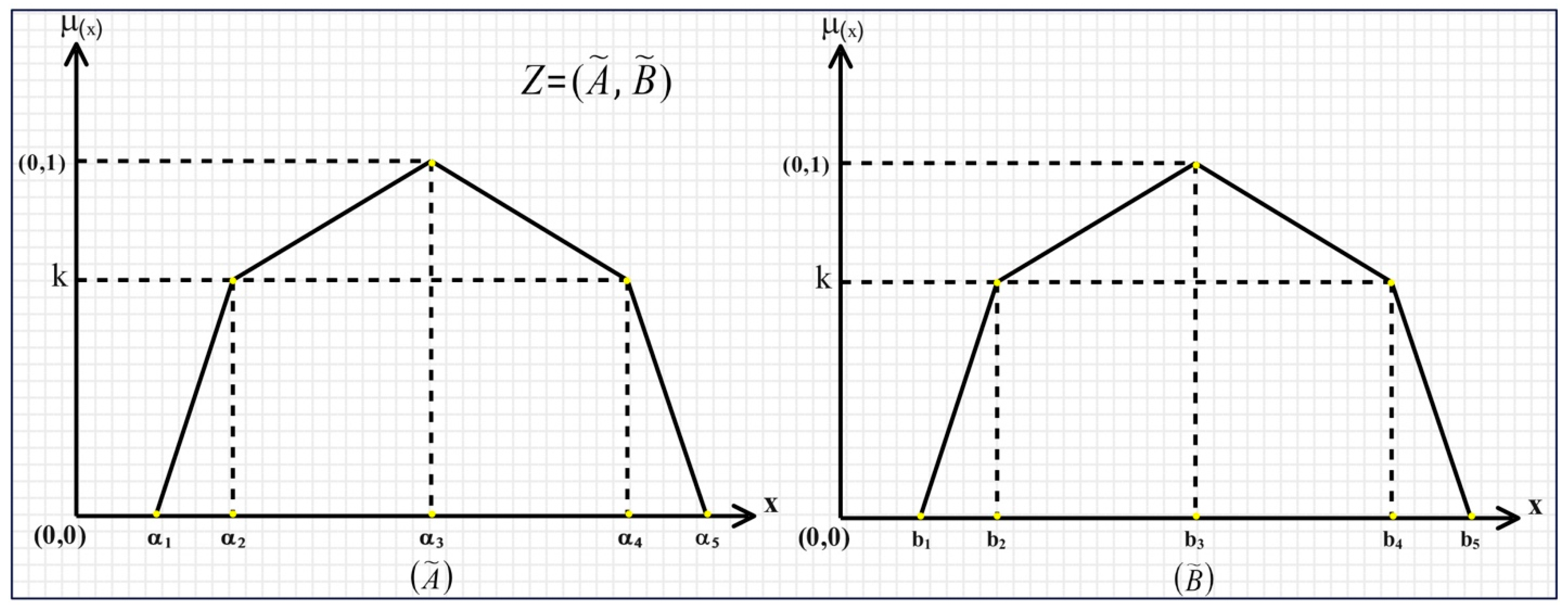
- Developing an integrated MCDM approach incorporating the PZ-LMAW and PZ-WASPAS methods to address combined uncertainty, utilizing the characteristics of symmetric and asymmetric POFNs, fuzzy constraint functions of Z-numbers, fuzzy reliability functions of Z-numbers, and the EI and EV concepts in symmetric and asymmetric POFNs.
- Proposing efficient approaches for calculating membership functions, a-cut formulations, and crispification processes for symmetric and asymmetric POFNs.
- Developing a robust and efficient decision support system capable of handling high levels of combined uncertainty in decision-making environments to address various MCDM and managerial issues.
- Conducting sensitivity analysis based on diverse approaches in the literature to validate and ensure the reliability of the results obtained through the proposed approach.
2. Literature Review
3. Materials and Methods
3.1. Preliminaries
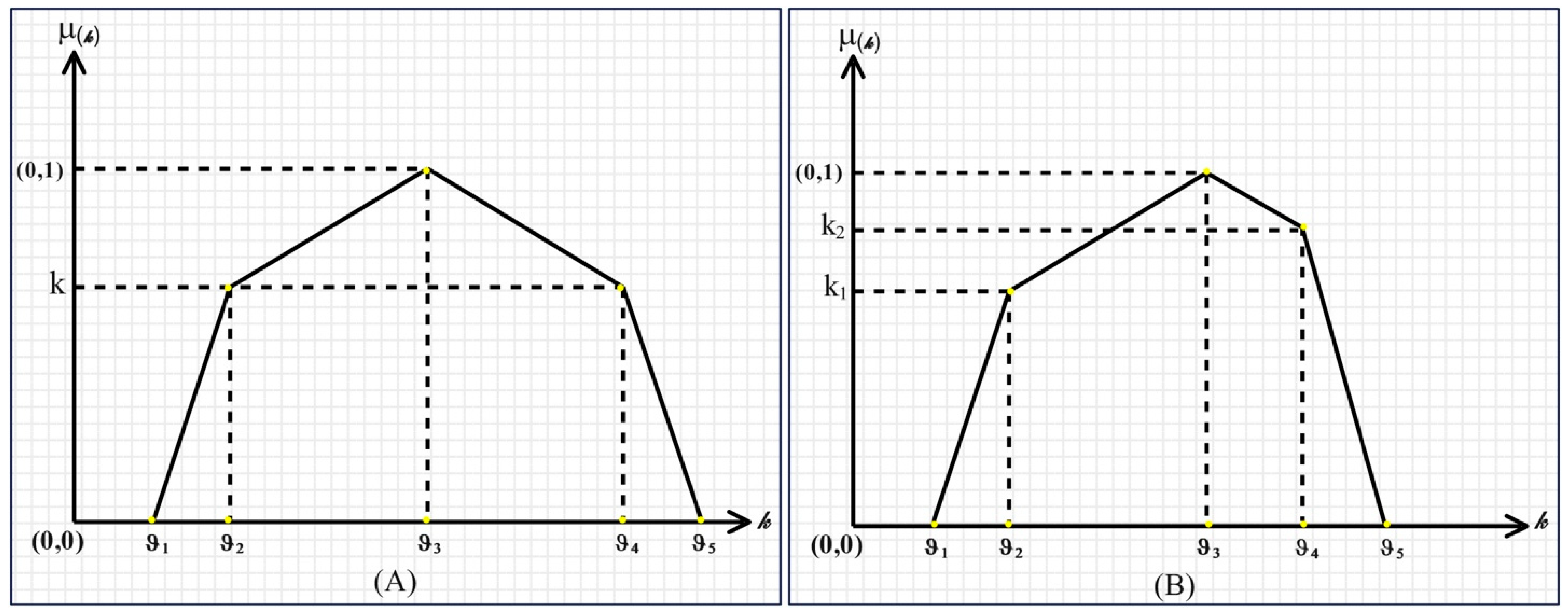
- is a convex fuzzy set.
- is normal, meaning there exists at least one such that the membership function .
- The membership function is piecewise continuous.
- For every , the of , denoted as , forms a closed interval.
- The support of , , is bounded.
- The membership function is continuous over the interval .
- The membership function is strictly a non-decreasing continuous function on the intervals and .
- The membership function is strictly a non-increasing continuous function on the intervals and .
- The starting point is first determined.
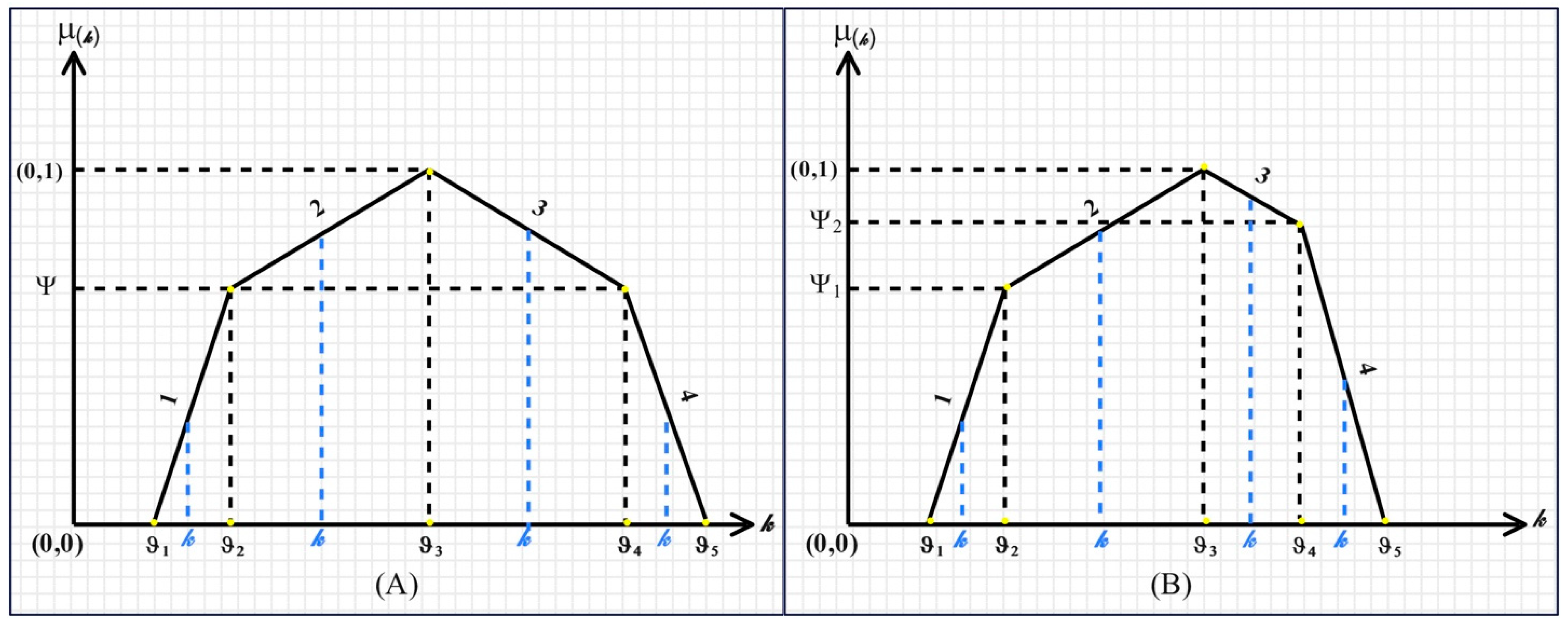
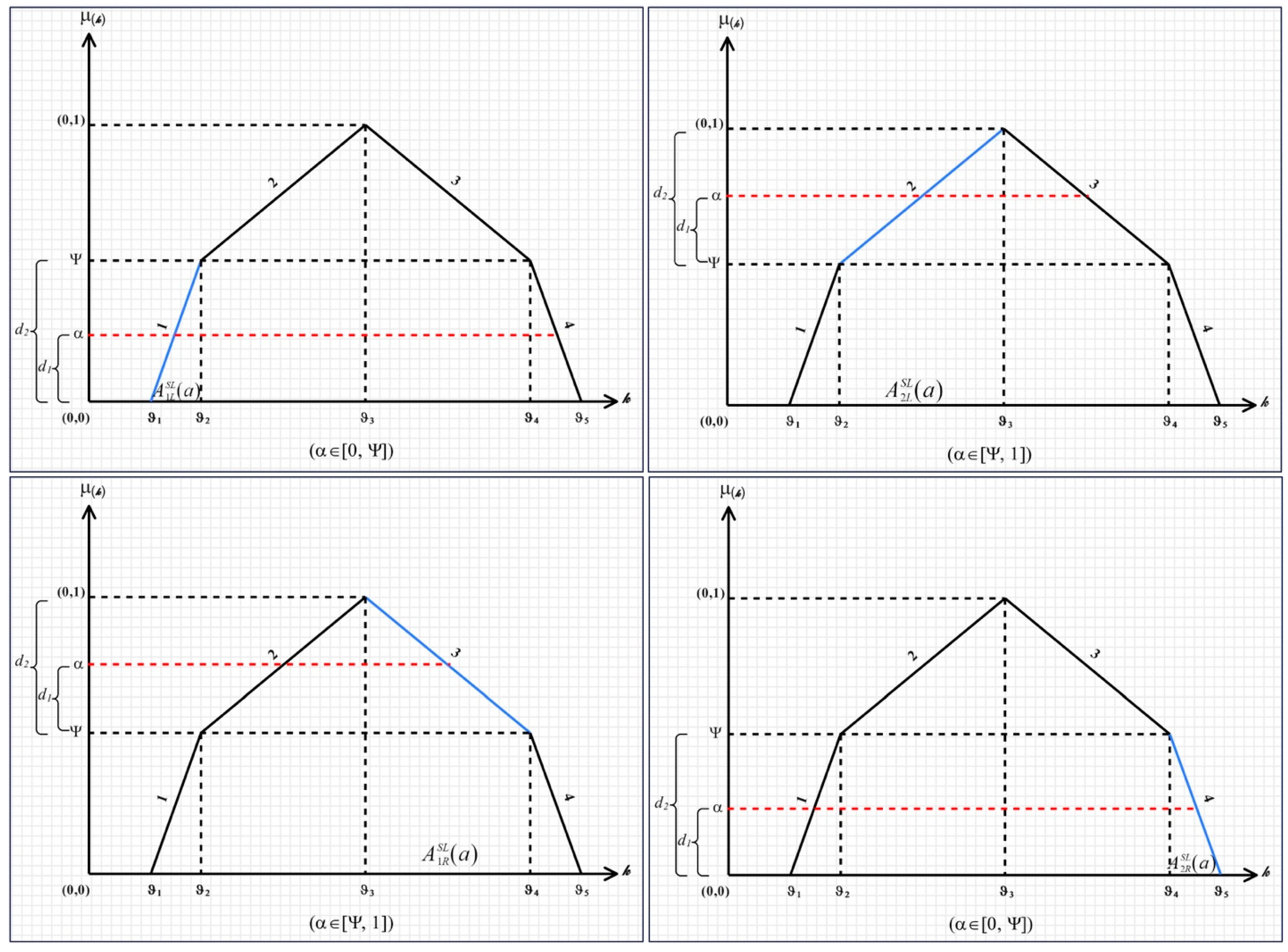
- The first distance () is divided by the second distance () and multiplied by the distance under the linear curve (according to Figure 3, for each of the linear curves 1, 2, 3, and 4, the distance under the curve corresponds to , , , and , respectively).
- Adding the results from steps 1 and 2 yields the -cut formula for the specified interval and linear curve.
- The starting point is first determined.
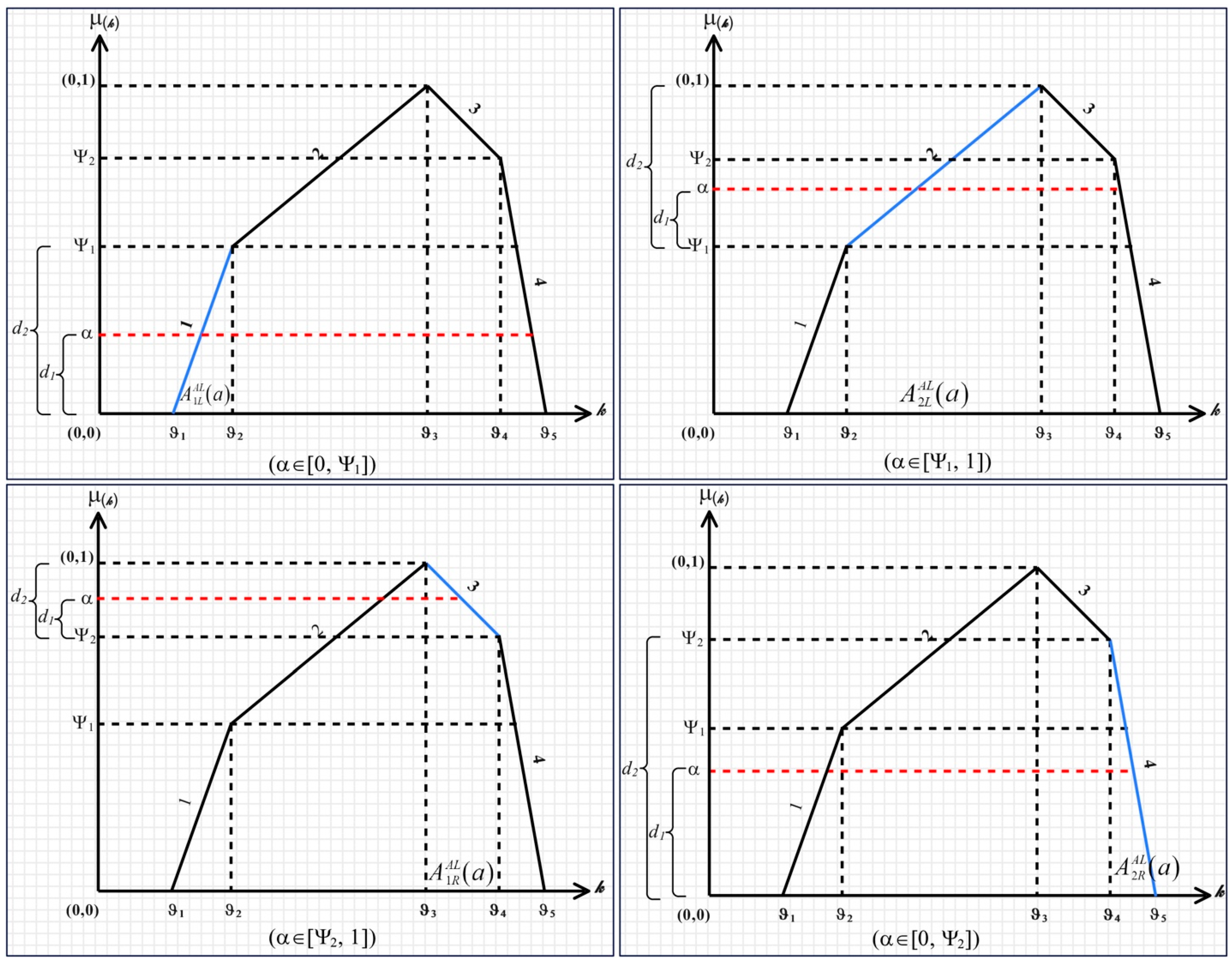
- The first distance () is divided by the second distance () and multiplied by the distance under the linear curve (according to Figure 4, for each of the linear curves 1, 2, 3, and 4, the distance under the curve corresponds to , , , and , respectively).
- Adding the results from steps 1 and 2 gives the -cut formula for the specified interval and linear curve.
3.2. The Crispification of POFNs
3.3. The Proposed PZ-LMAW
3.4. The Proposed PZ-WASPAS
4. Case Study and Results
4.1. Calculation of the Importance of SES Criteria
4.2. Prioritization of Smart Logistic Suppliers
5. Validation of the Results
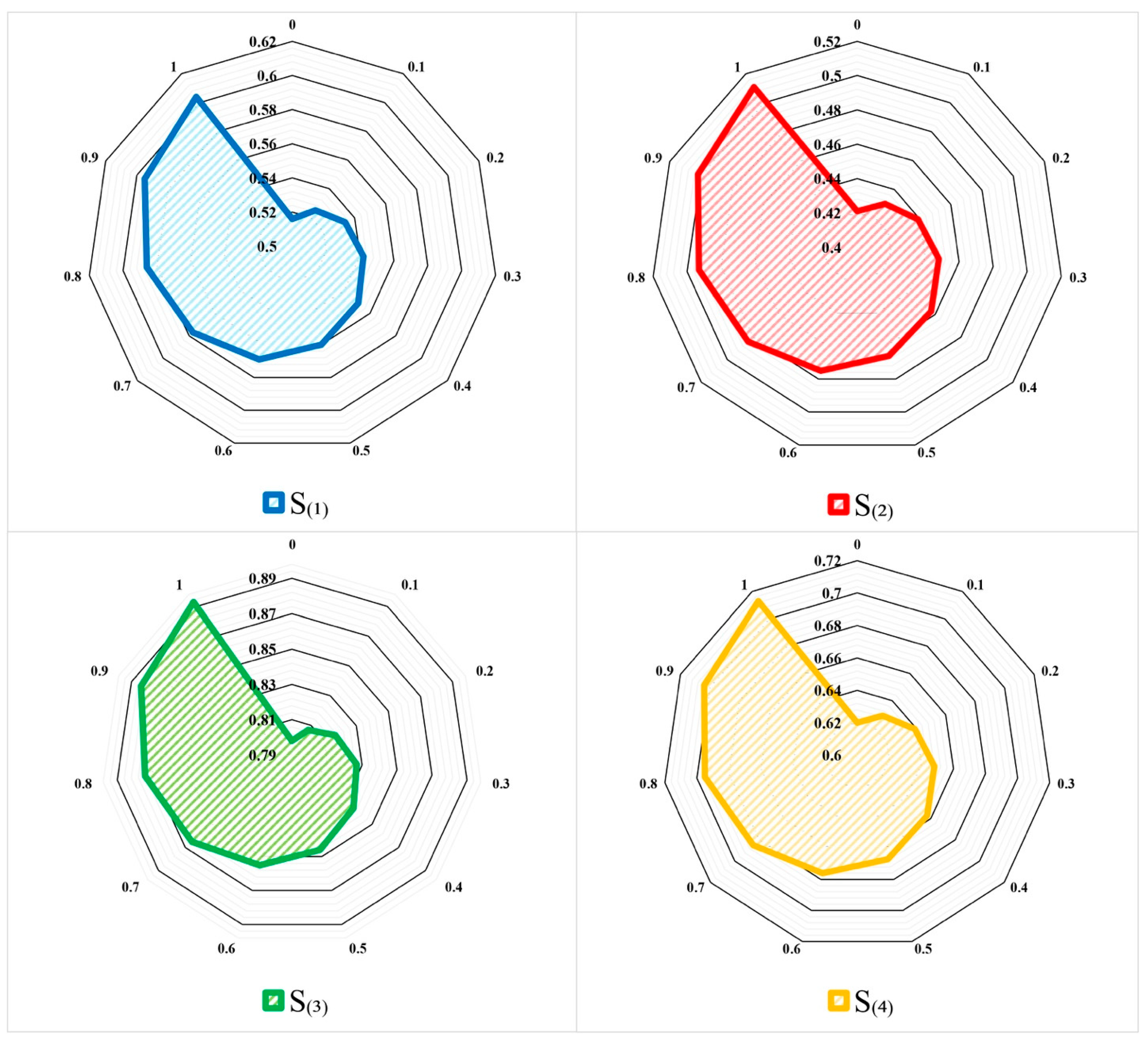
5.1. Sensitivity Analysis Based on the WASPAS Measure
5.2. Sensitivity Analysis Based on the Logical Pattern
5.3. Comparative Analysis
6. Discussion
7. Conclusions
Author Contributions
Funding
Data Availability Statement
Conflicts of Interest
References
- Tjahjono, B.; Esplugues, C.; Ares, E.; Pelaez, G. What Does Industry 4.0 Mean to Supply Chain? Procedia Manuf. 2017, 13, 1175–1182. [Google Scholar] [CrossRef]
- Mokhtarzadeh, N.G.; Jafarpanah, I.; Babgohari, A.Z. The Impact of international networking capability on international performance: The mediating role of dynamic entrepreneurship capabilities. In Empirical International Entrepreneurship: A Handbook of Methods, Approaches and Applications; Springer: Berlin/Heidelberg, Germany, 2021; pp. 307–336. [Google Scholar]
- Alaloul, W.S.; Liew, M.S.; Zawawi, N.A.W.A.; Kennedy, I.B. Industrial Revolution 4.0 in the Construction Industry: Challenges and Opportunities for Stakeholders. Ain Shams Eng. J. 2020, 11, 225–230. [Google Scholar] [CrossRef]
- Da Silva, V.L.; Kovaleski, J.L.; Pagani, R.N. Technology Transfer in the Supply Chain Oriented to Industry 4.0: A Literature Review. Technol. Anal. Strat. Manag. 2019, 31, 546–562. [Google Scholar] [CrossRef]
- Bai, C.; Kusi-Sarpong, S.; Badri Ahmadi, H.; Sarkis, J. Social Sustainable Supplier Evaluation and Selection: A Group Decision-Support Approach. Int. J. Prod. Res. 2019, 57, 7046–7067. [Google Scholar] [CrossRef]
- Matthess, M.; Kunkel, S.; Xue, B.; Beier, G. Supplier Sustainability Assessment in the Age of Industry 4.0–Insights from the Electronics Industry. Clean. Logist. Supply Chain. 2022, 4, 100038. [Google Scholar] [CrossRef]
- Hasan, M.M.; Jiang, D.; Ullah, A.M.M.S.; Noor-E-Alam, M. Resilient Supplier Selection in Logistics 4.0 with Heterogeneous Information. Expert. Syst. Appl. 2020, 139, 112799. [Google Scholar] [CrossRef]
- Hashemi-Tabatabaei, M.; Amiri, M.; Keshavarz-Ghorabaee, M. Gresilient Supplier Evaluation and Selection under Uncertainty Using a Novel Streamlined Full Consistency Method. Logistics 2024, 8, 90. [Google Scholar] [CrossRef]
- Amiri, M.; Hashemi-Tabatabaei, M.; Ghahremanloo, M.; Keshavarz-Ghorabaee, M.; Zavadskas, E.K.; Banaitis, A. A New Fuzzy BWM Approach for Evaluating and Selecting a Sustainable Supplier in Supply Chain Management. Int. J. Sustain. Dev. World Ecol. 2021, 28, 125–142. [Google Scholar] [CrossRef]
- Büyüközkan, G.; Göçer, F. Digital Supply Chain: Literature Review and a Proposed Framework for Future Research. Comput. Ind. 2018, 97, 157–177. [Google Scholar] [CrossRef]
- Chen, Z.; Ming, X.; Zhou, T.; Chang, Y. Sustainable Supplier Selection for Smart Supply Chain Considering Internal and External Uncertainty: An Integrated Rough-Fuzzy Approach. Appl. Soft Comput. 2020, 87, 106004. [Google Scholar] [CrossRef]
- Jamwal, A.; Agrawal, R.; Sharma, M.; Kumar, V. Review on Multi-Criteria Decision Analysis in Sustainable Manufacturing Decision Making. Int. J. Sustain. Eng. 2021, 14, 202–225. [Google Scholar] [CrossRef]
- Khulud, K.; Masudin, I.; Zulfikarijah, F.; Restuputri, D.P.; Haris, A. Sustainable Supplier Selection through Multi-Criteria Decision Making (MCDM) Approach: A Bibliometric Analysis. Logistics 2023, 7, 96. [Google Scholar] [CrossRef]
- Guarnieri, P.; Trojan, F. Decision Making on Supplier Selection Based on Social, Ethical, and Environmental Criteria: A Study in the Textile Industry. Resour. Conserv. Recycl. 2019, 141, 347–361. [Google Scholar] [CrossRef]
- Demiralay, E.; Paksoy, T. Strategy Development for Supplier Selection Process with Smart and Sustainable Criteria in Fuzzy Environment. Clean. Logist. Supply Chain. 2022, 5, 100076. [Google Scholar] [CrossRef]
- Büyüközkan, G.; Göçer, F. An Extension of ARAS Methodology under Interval Valued Intuitionistic Fuzzy Environment for Digital Supply Chain. Appl. Soft Comput. 2018, 69, 634–654. [Google Scholar] [CrossRef]
- Fallahpour, A.; Udoncy Olugu, E.; Nurmaya Musa, S.; Yew Wong, K.; Noori, S. A Decision Support Model for Sustainable Supplier Selection in Sustainable Supply Chain Management. Comput. Ind. Eng. 2017, 105, 391–410. [Google Scholar] [CrossRef]
- Zaid, A.A.; Jaaron, A.A.M.; Bon, A.T. The Impact of Green Human Resource Management and Green Supply Chain Management Practices on Sustainable Performance: An Empirical Study. J. Clean. Prod. 2018, 204, 965–979. [Google Scholar] [CrossRef]
- Onoda, H. Smart Approaches to Waste Management for Post-COVID-19 Smart Cities in Japan. IET Smart Cities 2020, 2, 89–94. [Google Scholar] [CrossRef]
- Wu, T.-W.; Zhang, H.; Peng, W.; Lü, F.; He, P.-J. Applications of Convolutional Neural Networks for Intelligent Waste Identification and Recycling: A Review. Resour. Conserv. Recycl. 2023, 190, 106813. [Google Scholar] [CrossRef]
- Olawade, D.B.; Fapohunda, O.; Wada, O.Z.; Usman, S.O.; Ige, A.O.; Ajisafe, O.; Oladapo, B.I. Smart Waste Management: A Paradigm Shift Enabled by Artificial Intelligence. Waste Manag. Bull. 2024, 2, 244–263. [Google Scholar] [CrossRef]
- Tiwari, S.; Wee, H.-M.; Daryanto, Y. Big Data Analytics in Supply Chain. Management between 2010 and 2016: Insights to Industries. Comput. Ind. Eng. 2018, 115, 319–330. [Google Scholar] [CrossRef]
- Laghari, J.A.; Mokhlis, H.; Bakar, A.H.A.; Mohammad, H. A Comprehensive Overview of New Designs in the Hydraulic, Electrical Equipments and Controllers of Mini Hydro Power Plants Making It Cost Effective Technology. Renew. Sustain. Energy Rev. 2013, 20, 279–293. [Google Scholar] [CrossRef]
- Frank, A.G.; Dalenogare, L.S.; Ayala, N.F. Industry 4.0 Technologies: Implementation Patterns in Manufacturing Companies. Int. J. Prod. Econ. 2019, 210, 15–26. [Google Scholar] [CrossRef]
- Bai, C.; Sarkis, J. Integrating Sustainability into Supplier Selection with Grey System and Rough Set Methodologies. Int. J. Prod. Econ. 2010, 124, 252–264. [Google Scholar] [CrossRef]
- Amiri, M.; Hashemi-Tabatabaei, M.; Keshavarz-Ghorabaee, M.; Antucheviciene, J.; Šaparauskas, J.; Keramatpanah, M. Evaluation of Digital Banking Implementation Indicators and Models in the Context of Industry 4.0: A Fuzzy Group MCDM Approach. Axioms 2023, 12, 516. [Google Scholar] [CrossRef]
- Çalık, A. A Novel Pythagorean Fuzzy AHP and Fuzzy TOPSIS Methodology for Green Supplier Selection in the Industry 4.0 Era. Soft Comput. 2021, 25, 2253–2265. [Google Scholar] [CrossRef]
- Kaur, H.; Singh, S.P. Multi-Stage Hybrid Model for Supplier Selection and Order Allocation Considering Disruption Risks and Disruptive Technologies. Int. J. Prod. Econ. 2021, 231, 107830. [Google Scholar] [CrossRef]
- Sharma, M.; Joshi, S. Digital Supplier Selection Reinforcing Supply Chain Quality Management Systems to Enhance Firm’s Performance. TQM J. 2023, 35, 102–130. [Google Scholar] [CrossRef]
- Torğul, B.; Paksoy, T. Smart and Sustainable Supplier Selection Using Interval Type-2 Fuzzy AHP. Politeknik Dergisi 2022, 1, 1. [Google Scholar]
- Ali, H.; Zhang, J.; Shoaib, M. A Hybrid Approach for Sustainable-Circular Supplier Selection Based on Industry 4.0 Framework to Make the Supply Chain Smart and Eco-Friendly. Environ. Dev. Sustain. 2023, 26, 1–38. [Google Scholar] [CrossRef]
- Xu, X.; Gu, J.; Yan, H.; Liu, W.; Qi, L.; Zhou, X. Reputation-Aware Supplier Assessment for Blockchain-Enabled Supply Chain in Industry 4.0. IEEE Trans. Ind. Inform. 2022, 19, 5485–5494. [Google Scholar] [CrossRef]
- Bonab, S.R.; Haseli, G.; Rajabzadeh, H.; Ghoushchi, S.J.; Hajiaghaei-Keshteli, M.; Tomaskova, H. Sustainable Resilient Supplier Selection for IoT Implementation Based on the Integrated BWM and TRUST under Spherical Fuzzy Sets. Decis. Mak. Appl. Manag. Eng. 2023, 6, 153–185. [Google Scholar] [CrossRef]
- Zekhnini, K.; Cherrafi, A.; Bouhaddou, I.; Benghabrit, Y.; Garza-Reyes, J.A. Supplier Selection for Smart Supply Chain: An adaptive fuzzy-neuro approach. In Proceedings of the 5th North America International Conference on Industrial Engineering and Operations Management (IEOM), Virtual, 10–14 August 2020; p. 92922. [Google Scholar]
- Kusi-Sarpong, S.; Gupta, H.; Khan, S.A.; Chiappetta Jabbour, C.J.; Rehman, S.T.; Kusi-Sarpong, H. Sustainable Supplier Selection Based on Industry 4.0 Initiatives within the Context of Circular Economy Implementation in Supply Chain Operations. Prod. Plan. Control 2023, 34, 999–1019. [Google Scholar] [CrossRef]
- Ghadimi, P.; Wang, C.; Lim, M.K.; Heavey, C. Intelligent Sustainable Supplier Selection Using Multi-Agent Technology: Theory and Application for Industry 4.0 Supply Chains. Comput. Ind. Eng. 2019, 127, 588–600. [Google Scholar] [CrossRef]
- Gai, T.; Cao, M.; Chiclana, F.; Wu, J.; Liang, C.; Herrera-Viedma, E. A Decentralized Feedback Mechanism with Compromise Behavior for Large-Scale Group Consensus Reaching Process with Application in Smart Logistics Supplier Selection. Expert. Syst. Appl. 2022, 204, 117547. [Google Scholar] [CrossRef]
- Tavana, M.; Sorooshian, S.; Mina, H. An Integrated Group Fuzzy Inference and Best–Worst Method for Supplier Selection in Intelligent Circular Supply Chains. Ann. Oper. Res. 2023, 342, 1–42. [Google Scholar] [CrossRef]
- Sachdeva, N.; Shrivastava, A.K.; Chauhan, A. Modeling Supplier Selection in the Era of Industry 4.0. Benchmarking Int. J. 2021, 28, 1809–1836. [Google Scholar] [CrossRef]
- Hosseini Dolatabad, A.; Heidary Dahooie, J.; Antucheviciene, J.; Azari, M.; Razavi Hajiagha, S.H. Supplier Selection in the Industry 4.0 Era by Using a Fuzzy Cognitive Map and Hesitant Fuzzy Linguistic VIKOR Methodology. Environ. Sci. Pollut. Res. 2023, 30, 52923–52942. [Google Scholar] [CrossRef] [PubMed]
- Liao, H.; Wen, Z.; Liu, L. Integrating BWM and ARAS under Hesitant Linguistic Environment for Digital Supply Chain Finance Supplier Section. Technol. Econ. Dev. Econ. 2019, 25, 1188–1212. [Google Scholar] [CrossRef]
- Kayapinar Kaya, S.; Aycin, E. An Integrated Interval Type 2 Fuzzy AHP and COPRAS-G Methodologies for Supplier Selection in the Era of Industry 4.0. Neural Comput. Appl. 2021, 33, 10515–10535. [Google Scholar] [CrossRef]
- Fallahpour, A.; Wong, K.Y.; Rajoo, S.; Fathollahi-Fard, A.M.; Antucheviciene, J.; Nayeri, S. An Integrated Approach for a Sustainable Supplier Selection Based on Industry 4.0 Concept. Environ. Sci. Pollut. Res. 2021, 2021, 1–19. [Google Scholar] [CrossRef] [PubMed]
- Fallahpour, A.; Yazdani, M.; Mohammed, A.; Wong, K.Y. Green Sourcing in the Era of Industry 4.0: Towards Green and Digitalized Competitive Advantages. Ind. Manag. Data Syst. 2021, 121, 1997–2025. [Google Scholar] [CrossRef]
- Camci, A.; Ertürk, M.E.; Gül, S. A novel fermatean fuzzy analytic hierarchy process proposition and its usage for supplier selection problem in industry 4.0 transition. In q-Rung Orthopair Fuzzy Sets: Theory and Applications; Springer: Berlin/Heidelberg, Germany, 2022; pp. 405–437. [Google Scholar]
- Wang, C.-N.; Nguyen, T.T.T.; Dang, T.-T.; Nguyen, N.-A.-T. A Hybrid OPA and Fuzzy MARCOS Methodology for Sustainable Supplier Selection with Technology 4.0 Evaluation. Processes 2022, 10, 2351. [Google Scholar] [CrossRef]
- ForouzeshNejad, A.A. Leagile and Sustainable Supplier Selection Problem in the Industry 4.0 Era: A Case Study of the Medical Devices Using Hybrid Multi-Criteria Decision Making Tool. Environ. Sci. Pollut. Res. 2023, 30, 13418–13437. [Google Scholar] [CrossRef]
- Zadeh, L.A. Fuzzy Sets. Inf. Control 1965, 8, 338–353. [Google Scholar] [CrossRef]
- Mondal, S.P.; Mandal, M. Pentagonal Fuzzy Number, Its Properties and Application in Fuzzy Equation. Future Comput. Inform. J. 2017, 2, 110–117. [Google Scholar] [CrossRef]
- Chakraborty, A.; Mondal, S.P.; Alam, S.; Ahmadian, A.; Senu, N.; De, D.; Salahshour, S. The Pentagonal Fuzzy Number: Its Different Representations, Properties, Ranking, Defuzzification and Application in Game Problems. Symmetry 2019, 11, 248. [Google Scholar] [CrossRef]
- Panda, A.; Pal, M. A Study on Pentagonal Fuzzy Number and Its Corresponding Matrices. Pac. Sci. Rev. B Humanit. Soc. Sci. 2015, 1, 131–139. [Google Scholar] [CrossRef]
- Zadeh, L.A. A Note on Z-Numbers. Inf. Sci. 2011, 181, 2923–2932. [Google Scholar] [CrossRef]
- Kang, B.; Wei, D.; Li, Y.; Deng, Y. Decision Making Using Z-Numbers under Uncertain Environment. J. Comput. Inf. Syst. 2012, 8, 2807–2814. [Google Scholar]
- Zheng, Q.; Liu, X.; Wang, W.; Han, S. A Hybrid HFACS Model Using DEMATEL-ORESTE Method with Linguistic Z-Number for Risk Analysis of Human Error Factors in the Healthcare System. Expert. Syst. Appl. 2024, 235, 121237. [Google Scholar] [CrossRef]
- Sari, I.U. Fermatean Fuzzy Z-Analytic Hierarchy Process: An Application to Third Party Logistics Providers. Eng. Appl. Artif. Intell. 2024, 133, 108327. [Google Scholar] [CrossRef]
- Arman, H. Fuzzy Analytic Hierarchy Process for Pentagonal Fuzzy Numbers and Its Application in Sustainable Supplier Selection. J. Clean. Prod. 2023, 409, 137190. [Google Scholar] [CrossRef]
- Jiménez, M.; Arenas, M.; Bilbao, A.; Rodrı, M.V. Linear Programming with Fuzzy Parameters: An Interactive Method Resolution. Eur. J. Oper. Res. 2007, 177, 1599–1609. [Google Scholar] [CrossRef]
- Heilpern, S. The Expected Value of a Fuzzy Number. Fuzzy Sets Syst. 1992, 47, 81–86. [Google Scholar] [CrossRef]
- Pamučar, D.; Žižović, M.; Biswas, S.; Božanić, D. A New Logarithm Methodology of Additive Weights (LMAW) for Multi-Criteria Decision-Making: Application in Logistics. Facta Univ. Ser. Mech. Eng. 2021, 19, 361–380. [Google Scholar] [CrossRef]
- Puška, A.; Božanić, D.; Nedeljković, M.; Janošević, M. Green Supplier Selection in an Uncertain Environment in Agriculture Using a Hybrid MCDM Model: Z-Numbers–Fuzzy LMAW–Fuzzy CRADIS Model. Axioms 2022, 11, 427. [Google Scholar] [CrossRef]
- Božanić, D.; Pamučar, D.; Milić, A.; Marinković, D.; Komazec, N. Modification of the Logarithm Methodology of Additive Weights (LMAW) by a Triangular Fuzzy Number and Its Application in Multi-Criteria Decision Making. Axioms 2022, 11, 89. [Google Scholar] [CrossRef]
- Puška, A.; Štilić, A.; Nedeljković, M.; Božanić, D.; Biswas, S. Integrating Fuzzy Rough Sets with LMAW and MABAC for Green Supplier Selection in Agribusiness. Axioms 2023, 12, 746. [Google Scholar] [CrossRef]
- Kang, B.; Wei, D.; Li, Y.; Deng, Y. A Method of Converting Z-Number to Classical Fuzzy Number. J. Inf. Comput. Sci. 2012, 9, 703–709. [Google Scholar]
- Bobar, Z.; Božanić, D.; Djurić, K.; Pamučar, D. Ranking and Assessment of the Efficiency of Social Media Using the Fuzzy AHP-Z Number Model-Fuzzy MABAC. Acta Polytech. Hung. 2020, 17, 43–70. [Google Scholar] [CrossRef]
- Stević, Ž.; Zavadskas, E.K.; Tawfiq, F.M.O.; Tchier, F.; Davidov, T. Fuzzy Multicriteria Decision-Making Model Based on Z Numbers for the Evaluation of Information Technology for Order Picking in Warehouses. Appl. Sci. 2022, 12, 12533. [Google Scholar] [CrossRef]
- Vojinović, N.; Stević, Ž.; Tanackov, I. A Novel IMF SWARA-FDWGA-PESTEL Analysis for Assessment of Healthcare System. Oper. Res. Eng. Sci. Theory Appl. 2022, 5, 139–151. [Google Scholar] [CrossRef]
- Pamucar, D. Normalized Weighted Geometric Dombi Bonferroni Mean Operator with Interval Grey Numbers: Application in Multicriteria Decision Making. Rep. Mech. Eng. 2020, 1, 44–52. [Google Scholar] [CrossRef]
- Zavadskas, E.K.; Turskis, Z.; Antucheviciene, J.; Zakarevicius, A. Optimization of Weighted Aggregated Sum Product Assessment. Elektron. Ir. Elektrotechnika 2012, 122, 3–6. [Google Scholar] [CrossRef]
- Chakraborty, S.; Zavadskas, E.K. Applications of WASPAS Method in Manufacturing Decision Making. Informatica 2014, 25, 1–20. [Google Scholar] [CrossRef]
- Chakraborty, S.; Zavadskas, E.K.; Antuchevičienė, J. Applications of WASPAS Method as a Multi-Criteria Decision-Making Tool. Econ. Comp. Econ. Cybern. Stud. Res. 2015, 49, 5–22. [Google Scholar]
- Mardani, A.; Nilashi, M.; Zakuan, N.; Loganathan, N.; Soheilirad, S.; Saman, M.Z.M.; Ibrahim, O. A Systematic Review and Meta-Analysis of SWARA and WASPAS Methods: Theory and Applications with Recent Fuzzy Developments. Appl. Soft Comput. 2017, 57, 265–292. [Google Scholar] [CrossRef]
- Turskis, Z.; Zavadskas, E.K.; Antuchevičienė, J.; Kosareva, N. A Hybrid Model Based on Fuzzy AHP and Fuzzy WASPAS for Construction Site Selection. Int. J. Comput. Commun. Control. 2015, 10, 113–128. [Google Scholar] [CrossRef]
- Rahmati, S.; Mahdavi, M.H.; Ghoushchi, S.J.; Tomaskova, H.; Haseli, G. Assessment and Prioritize Risk Factors of Financial Measurement of Management Control System for Production Companies Using a Hybrid Z-SWARA and Z-WASPAS with FMEA Method: A Meta-Analysis. Mathematics 2022, 10, 253. [Google Scholar] [CrossRef]
- Demir, G.; Chatterjee, P.; Pamucar, D. Sensitivity Analysis in Multi-Criteria Decision Making: A State-of-the-Art Research Perspective Using Bibliometric Analysis. Expert. Syst. Appl. 2024, 237, 121660. [Google Scholar] [CrossRef]
- Keshavarz Ghorabaee, M.; Amiri, M.; Zavadskas, E.K.; Turskis, Z.; Antucheviciene, J. Stochastic EDAS Method for Multi-Criteria Decision-Making with Normally Distributed Data. J. Intell. Fuzzy Syst. 2017, 33, 1627–1638. [Google Scholar] [CrossRef]
- Keshavarz-Ghorabaee, M.; Amiri, M.; Hashemi-Tabatabaei, M.; Zavadskas, E.K.; Kaklauskas, A. A New Decision-Making Approach Based on Fermatean Fuzzy Sets and WASPAS for Green Construction Supplier Evaluation. Mathematics 2020, 8, 2202. [Google Scholar] [CrossRef]
- Chen, J.; Wang, J.; Baležentis, T.; Zagurskaitė, F.; Streimikiene, D.; Makutėnienė, D. Multicriteria Approach towards the Sustainable Selection of a Teahouse Location with Sensitivity Analysis. Sustainability 2018, 10, 2926. [Google Scholar] [CrossRef]
- Zavadskas, E.K.; Chakraborty, S.; Bhattacharyya, O.; Antuchevičienė, J. Application of WASPAS Method as an Optimization Tool in Non-traditional Machining Processes. Inf. Technol. Control. 2015, 44, 77–88. [Google Scholar] [CrossRef]


| No. | Studies | Methodology/Approach | Information Type | Application Area |
|---|---|---|---|---|
| 1 | Demiralay et al. [15] | BWM, AHP, TOPSIS | Pythagorean fuzzy sets | Automobile spare parts |
| 2 | Çalık [27] | AHP, TOPSIS | Pythagorean fuzzy sets | Agricultural tools |
| 3 | Chen et al. [11] | DEMATEL, TOPSIS | Rough–fuzzy | Vehicle transmission system |
| 4 | Kaur et al. [28] | DEA, AHP, TOPSIS, MIP | Triangular fuzzy numbers | Automobile |
| 5 | Sharma et al. [29] | SWARA, WASPAS | Crisp values | Manufacturing firms |
| 6 | Torğul et al. [30] | AHP | Interval type-2 fuzzy sets | Automobile |
| 7 | Ali et al. [31] | FUCOM, MULTIMOORA | Triangular fuzzy numbers | Beverage |
| 8 | Xu et al. [32] | Classification, neural networks | Crisp values | Blockchain |
| 9 | Bonab et al. [33] | BWM, TRUST | Spherical fuzzy sets | IoT |
| 10 | Zekhnini et al. [34] | Adaptive fuzzy-neuro system | Fuzzy sets | Digital supply chain |
| 11 | Kusi-Sarpong et al. [35] | BWM, VIKOR | Crisp values | Textile |
| 12 | Ghadimi et al. [36] | Fuzzy inference system | Fuzzy sets | Medical devices |
| 13 | Gai et al. [37] | Large-scale group decision-making | 2-tuple linguistic | Smart logistics |
| 14 | Tavana et al. [38] | BWM, fuzzy inference system | Triangular fuzzy numbers | Offshore wind farm |
| 15 | Sachdeva et al. [39] | Entropy, TOPSIS | Intuitionistic fuzzy sets | Automobile |
| 16 | Hosseini Dolatabad et al. [40] | Fuzzy cognitive map, VIKOR | Hesitant fuzzy sets | Electronics |
| 17 | Liao et al. [41] | BWM, ARAS | Hesitant fuzzy sets | Finance |
| 18 | Hasan et al. [7] | Goal programming, TOPSIS | Triangular fuzzy numbers | Hypothetical case study |
| 19 | Kayapinar Kaya et al. [42] | AHP, COPRAS | Interval type-2 fuzzy sets, grey numbers | Textile |
| 20 | Fallahpour et al. [43] | BWM, fuzzy inference system | Triangular fuzzy numbers | Textile |
| 21 | Fallahpour et al. [44] | FPP, MOORA | Triangular fuzzy numbers | Food |
| 22 | Camci et al. [45] | AHP | Fermatean fuzzy sets | Industry 4.0 |
| 23 | Matthess et al. [6] | Interview-based approach | Qualitative | Electronics |
| 24 | Wang et al. [46] | OPA, MARCOS | Triangular fuzzy numbers | Leather and footwear |
| 25 | ForouzeshNejad [47] | BWM, MABAC | Rough sets | Medical devices |
| 26 | Current study | LMAW, WASPAS | Polygonal fuzzy Z-numbers | Home appliances |
| Linguistic Constraint | PFN Membership Function | Linguistic Reliability | PFN Membership Function |
|---|---|---|---|
| Extremely low (EL) | (1, 1, 1, 1, 1; 0.7) | Absolutely reliable (AR) | (0.8, 0.85, 0.9, 0.95, 1; 0.7) |
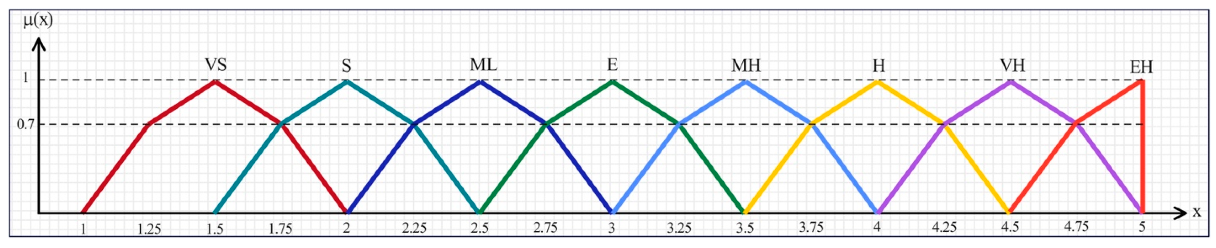
| Very slight (VS) | (1, 1.25, 1.5, 1.75, 2; 0.7) | Strongly reliable (SR) | (0.7, 0.75, 0.8, 0.85, 0.9; 0.7) |
| Slight (S) | (1.5, 1.75, 2, 2.25, 2.5; 0.7) | Very highly reliable (VR) | (0.6, 0.65, 0.7, 0.75, 0.8; 0.7) |
| Moderately low (ML) | (2, 2.25, 2.5, 2.75, 3; 0.7) | Highly reliable (HR) | (0.5, 0.55, 0.6, 0.65, 0.7; 0.7) |
| Equal (E) | (2.5, 2.75, 3, 3.25, 3.5; 0.7) | Fairly reliable (FR) | (0.4, 0.45, 0.5, 0.55, 0.6; 0.7) |
| Moderately high (MH) | (3, 3.25, 3.5, 3.75, 4; 0.7) | Weakly reliable (WR) | (0.3, 0.35, 0.4, 0.45, 0.5; 0.7) |
| High (H) | (3.5, 3.75, 4, 4.25, 4.5; 0.7) | Very weakly reliable (VW) | (0.2, 0.25, 0.3, 0.35, 0.4; 0.7) |
| Very high (VH) | (4, 4.25, 4.5, 4.75, 5; 0.7) | Strongly unreliable (SU) | (0.1, 0.15, 0.2, 0.25, 0.3; 0.7) |
| Extremely high (EH) | (4.5, 4.75, 5, 5, 5; 0.7) | Absolutely unreliable (AU) | (0, 0, 0, 0, 0.2; 0.7) |
| Linguistic Constraint | PFN Membership Function | Crisp | Linguistic Reliability | PFN Membership Function |
|---|---|---|---|---|
| Extremely low (EL) | (1, 1, 1, 1, 1; 0.6, 0.8) | Absolutely reliable (AR) | (0.8, 0.85, 0.9, 0.95, 1; 0.6, 0.8) | |
| Very low (VL) | (1, 1, 2, 3, 4; 0.6, 0.8) | Strongly reliable (SR) | (0.7, 0.75, 0.8, 0.85, 9; 0.6, 0.8) | |
| Low (L) | (1, 2, 3, 4, 5; 0.6, 0.8) | Very highly reliable (VR) | (0.6, 0.65, 0.7, 0.75, 0.8; 0.6, 0.8) | |
| Slightly below average (SB) | (2, 3, 4, 5, 6; 0.6, 0.8) | Highly reliable (HR) | (0.5, 0.55, 0.6, 0.65, 0.7; 0.6, 0.8) | |
| Average (A) | (3, 4, 5, 6, 7; 0.6, 0.8) | Fairly reliable (FR) | (0.4, 0.45, 0.5, 0.55, 0.6; 0.6, 0.8) | |
| Slightly above average (SA) | (4, 5, 6, 7, 8; 0.6, 0.8) | Weakly reliable (WR) | (0.3, 0.35, 0.4, 0.45, 0.5; 0.6, 0.8) | |
| High (H) | (5, 6, 7, 8, 9; 0.6, 0.8) | Very weakly reliable (VW) | (0.2, 0.25, 0.3, 0.35, 0.4; 0.6, 0.8) | |
| Very high (VH) | (6, 7, 8, 9, 9; 0.6, 0.8) | Strongly unreliable (SU) | (0.1, 0.15, 0.2, 0.25, 0.3; 0.6, 0.8) | |
| Extremely high (EH) | (7, 8, 9, 10, 10; 0.6, 0.8) | Absolutely unreliable (AU) | (0, 0, 0, 0, 0.2; 0.6, 0.8) |
| Experts | Education | Specialized Area | Field | Position | Experience | |
|---|---|---|---|---|---|---|
| Ph.D. | MA | |||||
| E(A) | ✓ | Industrial engineering | Industry | Chief procurement officer | 20+ | |
| E(B) | ✓ | Production planning | Industry | Production manager | 25+ | |
| E(C) | ✓ | Industrial management | Academic | Faculty member | 15+ | |
| Sustainable Smart SES Criteria | Supplier Requirements | References |
|---|---|---|
| C1: Employee development in a smart environment | Suppliers foster employee development by providing training in smart technologies, offering flexible work arrangements, and creating opportunities for professional growth. | [11,25,26] |
| C2: Green and smart logistics and manufacturing | Suppliers adopt smart technologies and advanced management practices to enhance energy efficiency, reduce emissions, and implement green logistics through solutions like smart electric vehicles and big data optimization. | [11,17,18] |
| C3: Waste reduction using smart technologies | Suppliers employ AI-driven recycling technologies to optimize material identification, sorting, and resource recovery, reducing waste contamination and improving sustainability in the supply chain. | [19,20,21] |
| C4: Cost reduction using smart technologies | Suppliers leverage smart technologies to reduce costs across the supply chain by employing IoT for real-time machine monitoring and using AI and big data analytics to minimize unplanned downtime and defects. | [22,23] |
| C5: Smart working environment | Suppliers create safe and smart working environments by utilizing tools like VR and AR for remote machine operations, ensuring employee safety and workplace health. | [16,24] |
| C6: Smart delivery to customer | Suppliers utilize smart tools to ensure timely product delivery by forecasting customer needs with AI (e.g., machine learning) and developing efficient production plans through reinforcement learning. | [10,11] |
| Experts | C1 | C2 | C3 | C4 | C5 | C6 |
|---|---|---|---|---|---|---|
| E(A) | ML, VR | H, SR | MH, SR | EH, SR | H, HR | ML, VR |
| E(B) | S, AR | EH, AR | VH, SR | H, AR | MH, SR | E, AR |
| E(C) | VS, VR | MH, SR | S, SR | VH, AR | H, AR | ML, SR |
| C1 | C2 | C3 | C4 | C5 | C6 | ||
|---|---|---|---|---|---|---|---|
| E(A) | 0.7 | 0.8 | 0.8 | 0.8 | 0.6 | 0.7 | |
| (1.67, 1.88, 2.09, 2.3, 2.5; 0.7) | (3.13, 3.35, 3.57, 3.8, 4.02; 0.7) | (2.68, 2.9, 3.13, 3.35, 3.57; 0.7) | (4.02, 4.24, 4.47, 4.47, 4.47; 0.7) | (2.71, 2.9, 3.09, 3.29, 3.48; 0.7) | (1.67, 1.88, 2.09, 2.3, 2.5; 0.7) | ||
| E(B) | 0.9 | 0.9 | 0.8 | 0.9 | 0.8 | 0.9 | |
| (1.42, 1.66, 1.89, 2.13, 2.37; 0.7) | (4.26, 4.5, 4.74, 4.74, 4.74; 0.7) | (3.57, 3.8, 4.02, 4.24, 4.47; 0.7) | (3.32, 3.55, 3.79, 4.03, 4.26; 0.7) | (2.68, 2.9, 3.13, 3.35, 3.57; 0.7) | (2.37, 2.6, 2.84, 3.08, 3.32; 0.7) | ||
| E(C) | 0.7 | 0.8 | 0.8 | 0.9 | 0.9 | 0.8 | |
| (0.83, 1.04, 1.25, 1.46, 1.67; 0.7) | (2.68, 2.9, 3.13, 3.35, 3.57; 0.7) | (1.34, 1.56, 1.78, 2.01, 2.23; 0.7) | (3.79, 4.03, 4.26, 4.5, 4.74; 0.7) | (3.32, 3.55, 3.79, 4.03, 4.26; 0.7) | (1.78, 2.01, 2.23, 2.45, 2.68; 0.7) | ||
| Experts | C1 | C2 | C3 | C4 | C5 | C6 |
|---|---|---|---|---|---|---|
| E(A) | (2, 2.45, 3, 3.66, 4.5; 0.7) | (3.74, 4.37, 5.13, 6.05, 7.21; 0.7) | (3.2, 3.79, 4.48, 5.34, 6.41; 0.7) | (4.81, 5.53, 6.41, 7.12, 8.01; 0.7) | (3.24, 3.78, 4.44, 5.24, 6.24; 0.7) | (2, 2.45, 3, 3.66, 4.5; 0.7) |
| E(B) | (1.8, 2.33, 3, 3.85, 5; 0.7) | (5.4, 6.33, 7.5, 8.57, 10; 0.7) | (4.52, 5.34, 6.36, 7.67, 9.42; 0.7) | (4.2, 5, 6, 7.28, 9; 0.7) | (3.39, 4.08, 4.94, 6.06, 7.54; 0.7) | (3, 3.66, 4.5, 5.57, 7; 0.7) |
| E(C) | (1.5, 2.14, 3, 4.2, 6; 0.7) | (4.81, 5.95, 7.48, 9.62, 12.82; 0.7) | (2.4, 3.2, 4.27, 5.77, 8.01; 0.7) | (6.8, 8.26, 10.2, 12.92, 17; 0.7) | (5.95, 7.28, 9.07, 11.56, 15.3; 0.7) | (3.2, 4.12, 5.34, 7.05, 9.62; 0.7) |
| C1 | C2 | C3 | C4 | C5 | C6 | |
|---|---|---|---|---|---|---|
| (0.04, 0.09, 0.11, 0.16, 0.22; 0.7) | (0.12, 0.18, 0.19, 0.24, 0.31; 0.7) | (0.08, 0.14, 0.16, 0.21, 0.28; 0.7) | (0.13, 0.19, 0.2, 0.25, 0.32; 0.7) | (0.11, 0.17, 0.17, 0.22, 0.29; 0.7) | (0.07, 0.12, 0.14, 0.19, 0.25; 0.7) | |
| 0.126 | 0.212 | 0.179 | 0.222 | 0.196 | 0.160 |
| Experts | Suppliers | C1 | C2 | C3 | C4 | C5 | C6 |
|---|---|---|---|---|---|---|---|
| E(A) | S(1) | H, SR | A, FR | SB, VR | A, FR | SB, VR | SA, VR |
| S(2) | H, AR | L, FR | SA, SR | SB, SR | A, HR | L, SR | |
| S(3) | SA, SR | EH, AR | SA, FR | EH, AR | H, SR | SA, SR | |
| S(4) | A, FR | VH, AR | SA, AR | H, AR | SB, FR | H, AR | |
| E(B) | S(1) | SB, VR | H, HR | SB, HR | A, VR | SA, SR | H, SR |
| S(2) | L, FR | A, HR | SA, FR | SA, FR | A, HR | SB, SR | |
| S(3) | SA, VR | VH, AR | A, VR | VH, AR | H, SR | VH, SR | |
| S(4) | SB, FR | SA, FR | SA, HR | EH, SR | VH, SR | SA, VR | |
| E(C) | S(1) | SA, FR | A, HR | SA, FR | H, SR | H, SR | A, SR |
| S(2) | VH, AR | SB, VR | A, FR | L, FR | H, FR | VH, SR | |
| S(3) | H, AR | EH, AR | H, AR | EH, AR | VH, SR | SA, VR | |
| S(4) | SA, SR | VH, AR | SA, SR | SA, VR | H, FR | A, VR | |
| Criteria | Experts | Suppliers | |||
|---|---|---|---|---|---|
| S(1) | S(2) | S(3) | S(4) | ||
| C1 | E(A) | (4.48, 5.38, 6.28, 7.17, 8.07; 0.6, 0.8) | (4.75, 5.7, 6.65, 7.61, 8.56; 0.6, 0.8) | (3.58, 4.48, 5.38, 6.28, 7.17; 0.6, 0.8) | (2.13, 2.84, 3.55, 4.26, 4.97; 0.6, 0.8) |
| E(B) | (1.67, 2.51, 3.35, 4.19, 5.03; 0.6, 0.8) | (0.71, 1.42, 2.13, 2.84, 3.55; 0.6, 0.8) | (3.35, 4.19, 5.03, 5.87, 6.71; 0.6, 0.8) | (1.42, 2.13, 2.84, 3.55, 4.26; 0.6, 0.8) | |
| E(C) | (2.84, 3.55, 4.26, 4.97, 5.68; 0.6, 0.8) | (5.7, 6.65, 7.61, 8.56, 8.56; 0.6, 0.8) | (4.75, 5.7, 6.65, 7.61, 8.56; 0.6, 0.8) | (3.58, 4.48, 5.38, 6.28, 7.17; 0.6, 0.8) | |
| C2 | E(A) | (2.13, 2.84, 3.55, 4.26, 4.97; 0.6, 0.8) | (0.71, 1.42, 2.13, 2.84, 3.55; 0.6, 0.8) | (6.65, 7.61, 8.56, 9.51, 9.51; 0.6, 0.8) | (5.7, 6.65, 7.61, 8.56, 8.56; 0.6, 0.8) |
| E(B) | (3.88, 4.66, 5.44, 6.22, 7; 0.6, 0.8) | (2.33, 3.11, 3.88, 4.66, 5.44; 0.6, 0.8) | (5.7, 6.65, 7.61, 8.56, 8.56; 0.6, 0.8) | (2.84, 3.55, 4.26, 4.97, 5.68; 0.6, 0.8) | |
| E(C) | (2.33, 3.11, 3.88, 4.66, 5.44; 0.6, 0.8) | (1.67, 2.51, 3.35, 4.19, 5.03; 0.6, 0.8) | (6.65, 7.61, 8.56, 9.51, 9.51; 0.6, 0.8) | (5.7, 6.65, 7.61, 8.56, 8.56; 0.6, 0.8) | |
| C3 | E(A) | (1.67, 2.51, 3.35, 4.19, 5.03; 0.6, 0.8) | (3.58, 4.48, 5.38, 6.28, 7.17; 0.6, 0.8) | (2.84, 3.55, 4.26, 4.97, 5.68; 0.6, 0.8) | (3.8, 4.75, 5.7, 6.65, 7.61; 0.6, 0.8) |
| E(B) | (1.55, 2.33, 3.11, 3.88, 4.66; 0.6, 0.8) | (2.84, 3.55, 4.26, 4.97, 5.68; 0.6, 0.8) | (2.51, 3.35, 4.19, 5.03, 5.87; 0.6, 0.8) | (3.11, 3.88, 4.66, 5.44, 6.22; 0.6, 0.8) | |
| E(C) | (2.84, 3.55, 4.26, 4.97, 5.68; 0.6, 0.8) | (2.13, 2.84, 3.55, 4.26, 4.97; 0.6, 0.8) | (4.75, 5.7, 6.65, 7.61, 8.56; 0.6, 0.8) | (3.58, 4.48, 5.38, 6.28, 7.17; 0.6, 0.8) | |
| C4 | E(A) | (2.13, 2.84, 3.55, 4.26, 4.97; 0.6, 0.8) | (1.79, 2.69, 3.58, 4.48, 5.38; 0.6, 0.8) | (6.65, 7.61, 8.56, 9.51, 9.51; 0.6, 0.8) | (4.75, 5.7, 6.65, 7.61, 8.56; 0.6, 0.8) |
| E(B) | (2.51, 3.35, 4.19, 5.03, 5.87; 0.6, 0.8) | (2.84, 3.55, 4.26, 4.97, 5.68; 0.6, 0.8) | (5.7, 6.65, 7.61, 8.56, 8.56; 0.6, 0.8) | (6.28, 7.17, 8.07, 8.97, 8.97; 0.6, 0.8) | |
| E(C) | (4.48, 5.38, 6.28, 7.17, 8.07; 0.6, 0.8) | (0.71, 1.42, 2.13, 2.84, 3.55; 0.6, 0.8) | (6.65, 7.61, 8.56, 9.51, 9.51; 0.6, 0.8) | (3.35, 4.19, 5.03, 5.87, 6.71; 0.6, 0.8) | |
| C5 | E(A) | (1.67, 2.51, 3.35, 4.19, 5.03; 0.6, 0.8) | (2.33, 3.11, 3.88, 4.66, 5.44; 0.6, 0.8) | (4.48, 5.38, 6.28, 7.17, 8.07; 0.6, 0.8) | (1.42, 2.13, 2.84, 3.55, 4.26; 0.6, 0.8) |
| E(B) | (3.58, 4.48, 5.38, 6.28, 7.17; 0.6, 0.8) | (2.33, 3.11, 3.88, 4.66, 5.44; 0.6, 0.8) | (4.48, 5.38, 6.28, 7.17, 8.07; 0.6, 0.8) | (5.38, 6.28, 7.17, 8.07, 8.07; 0.6, 0.8) | |
| E(C) | (4.48, 5.38, 6.28, 7.17, 8.07; 0.6, 0.8) | (3.55, 4.26, 4.97, 5.68, 6.39; 0.6, 0.8) | (5.38, 6.28, 7.17, 8.07, 8.07; 0.6, 0.8) | (3.55, 4.26, 4.97, 5.68, 6.39; 0.6, 0.8) | |
| C6 | E(A) | (3.35, 4.19, 5.03, 5.87, 6.71; 0.6, 0.8) | (0.89, 1.79, 2.69, 3.58, 4.48; 0.6, 0.8) | (3.58, 4.48, 5.38, 6.28, 7.17; 0.6, 0.8) | (4.75, 5.7, 6.65, 7.61, 8.56; 0.6, 0.8) |
| E(B) | (4.48, 5.38, 6.28, 7.17, 8.07; 0.6, 0.8) | (1.79, 2.69, 3.58, 4.48, 5.38; 0.6, 0.8) | (5.38, 6.28, 7.17, 8.07, 8.07; 0.6, 0.8) | (3.35, 4.19, 5.03, 5.87, 6.71; 0.6, 0.8) | |
| E(C) | (2.69, 3.58, 4.48, 5.38, 6.28; 0.6, 0.8) | (5.38, 6.28, 7.17, 8.07, 8.07; 0.6, 0.8) | (3.35, 4.19, 5.03, 5.87, 6.71; 0.6, 0.8) | (2.51, 3.35, 4.19, 5.03, 5.87; 0.6, 0.8) | |
| Criteria | Suppliers | |||
|---|---|---|---|---|
| S(1) | S(2) | S(3) | S(4) | |
| C1 | (2.56, 3.47, 4.33, 5.18, 6.02; 0.6, 0.8) | (1.67, 2.91, 3.99, 5, 5.82; 0.6, 0.8) | (3.81, 4.71, 5.61, 6.51, 7.4; 0.6, 0.8) | (2.06, 2.87, 3.66, 4.44, 5.21; 0.6, 0.8) |
| C2 | (2.59, 3.38, 4.15, 4.92, 5.68; 0.6, 0.8) | (1.23, 2.1, 2.92, 3.73, 4.52; 0.6, 0.8) | (6.3, 7.26, 8.21, 9.17, 9.17; 0.6, 0.8) | (4.27, 5.15, 6.03, 6.9, 7.32; 0.6, 0.8) |
| C3 | (1.88, 2.71, 3.51, 4.3, 5.09; 0.6, 0.8) | (2.72, 3.5, 4.27, 5.04, 5.81; 0.6, 0.8) | (3.12, 3.97, 4.81, 5.65, 6.48; 0.6, 0.8) | (3.47, 4.34, 5.21, 6.08, 6.95; 0.6, 0.8) |
| C4 | (2.75, 3.59, 4.41, 5.24, 6.06; 0.6, 0.8) | (1.29, 2.21, 3.05, 3.86, 4.66; 0.6, 0.8) | (6.3, 7.26, 8.21, 9.17, 9.17; 0.6, 0.8) | (4.49, 5.42, 6.34, 7.26, 7.95; 0.6, 0.8) |
| C5 | (2.73, 3.72, 4.66, 5.58, 6.49; 0.6, 0.8) | (2.63, 3.41, 4.19, 4.96, 5.72; 0.6, 0.8) | (4.75, 5.65, 6.55, 7.45, 8.07; 0.6, 0.8) | (2.56, 3.47, 4.33, 5.16, 5.82; 0.6, 0.8) |
| C6 | (3.36, 4.26, 5.16, 6.05, 6.94; 0.6, 0.8) | (1.61, 2.75, 3.8, 4.79, 5.63; 0.6, 0.8) | (3.93, 4.83, 5.72, 6.61, 7.28; 0.6, 0.8) | (3.31, 4.21, 5.11, 5.99, 6.88; 0.6, 0.8) |
| Criteria | Suppliers | |||
|---|---|---|---|---|
| S(1) | S(2) | S(3) | S(4) | |
| C1 | (0.346, 0.468, 0.585, 0.7, 0.812; 0.6, 0.8) | (0.225, 0.393, 0.539, 0.674, 0.786; 0.6, 0.8) | (0.514, 0.636, 0.757, 0.878, 1; 0.6, 0.8) | (0.279, 0.388, 0.494, 0.599, 0.704; 0.6, 0.8) |
| C2 | (0.283, 0.368, 0.452, 0.536, 0.619; 0.6, 0.8) | (0.134, 0.229, 0.319, 0.406, 0.492; 0.6, 0.8) | (0.687, 0.791, 0.896, 1, 1; 0.6, 0.8) | (0.465, 0.562, 0.657, 0.752, 0.798; 0.6, 0.8) |
| C3 | (0.271, 0.389, 0.505, 0.619, 0.732; 0.6, 0.8) | (0.392, 0.503, 0.614, 0.725, 0.835; 0.6, 0.8) | (0.449, 0.571, 0.692, 0.812, 0.932; 0.6, 0.8) | (0.5, 0.625, 0.75, 0.875, 1; 0.6, 0.8) |
| C4 | (0.3, 0.391, 0.481, 0.571, 0.66; 0.6, 0.8) | (0.141, 0.241, 0.332, 0.421, 0.508; 0.6, 0.8) | (0.687, 0.791, 0.896, 1, 1; 0.6, 0.8) | (0.49, 0.591, 0.692, 0.791, 0.867; 0.6, 0.8) |
| C5 | (0.338, 0.461, 0.578, 0.692, 0.804; 0.6, 0.8) | (0.326, 0.423, 0.519, 0.614, 0.709; 0.6, 0.8) | (0.588, 0.7, 0.811, 0.923, 1; 0.6, 0.8) | (0.317, 0.43, 0.536, 0.639, 0.721; 0.6, 0.8) |
| C6 | (0.461, 0.586, 0.709, 0.832, 0.953; 0.6, 0.8) | (0.221, 0.378, 0.521, 0.658, 0.773; 0.6, 0.8) | (0.54, 0.664, 0.786, 0.909, 1; 0.6, 0.8) | (0.455, 0.579, 0.702, 0.824, 0.945; 0.6, 0.8) |
| Suppliers | Order | ||||
|---|---|---|---|---|---|
| S(1) | (0.359, 0.478, 0.594, 0.708, 0.822; 0.6, 0.8) | (0.29, 0.398, 0.505, 0.613, 0.722; 0.6, 0.8) | (0.324, 0.438, 0.549, 0.661, 0.772; 0.6, 0.8) | 0.560 | 3 |
| S(2) | (0.258, 0.385, 0.504, 0.62, 0.728; 0.6, 0.8) | (0.187, 0.303, 0.413, 0.521, 0.624; 0.6, 0.8) | (0.222, 0.344, 0.459, 0.57, 0.676; 0.6, 0.8) | 0.466 | 4 |
| S(3) | (0.645, 0.769, 0.893, 1.016, 1.082; 0.6, 0.8) | (0.553, 0.674, 0.796, 0.919, 0.987; 0.6, 0.8) | (0.599, 0.722, 0.844, 0.967, 1.035; 0.6, 0.8) | 0.846 | 1 |
| S(4) | (0.467, 0.588, 0.707, 0.824, 0.922; 0.6, 0.8) | (0.384, 0.499, 0.613, 0.726, 0.821; 0.6, 0.8) | (0.425, 0.543, 0.66, 0.775, 0.872; 0.6, 0.8) | 0.667 | 2 |
| -Level | Suppliers | Order | |||
|---|---|---|---|---|---|
| S(1) | S(2) | S(3) | S(4) | ||
| 0.516 | 0.421 | 0.798 | 0.620 | S(3) S(4) S(1) S(2) | |
| 0.525 | 0.430 | 0.807 | 0.629 | S(3) S(4) S(1) S(2) | |
| 0.534 | 0.439 | 0.817 | 0.639 | S(3) S(4) S(1) S(2) | |
| 0.542 | 0.448 | 0.827 | 0.648 | S(3) S(4) S(1) S(2) | |
| 0.551 | 0.457 | 0.836 | 0.657 | S(3) S(4) S(1) S(2) | |
| 0.560 | 0.466 | 0.846 | 0.667 | S(3) S(4) S(1) S(2) | |
| 0.569 | 0.475 | 0.855 | 0.676 | S(3) S(4) S(1) S(2) | |
| 0.577 | 0.484 | 0.865 | 0.685 | S(3) S(4) S(1) S(2) | |
| 0.586 | 0.493 | 0.874 | 0.695 | S(3) S(4) S(1) S(2) | |
| 0.595 | 0.502 | 0.884 | 0.704 | S(3) S(4) S(1) S(2) | |
| 0.604 | 0.511 | 0.893 | 0.713 | S(3) S(4) S(1) S(2) | |
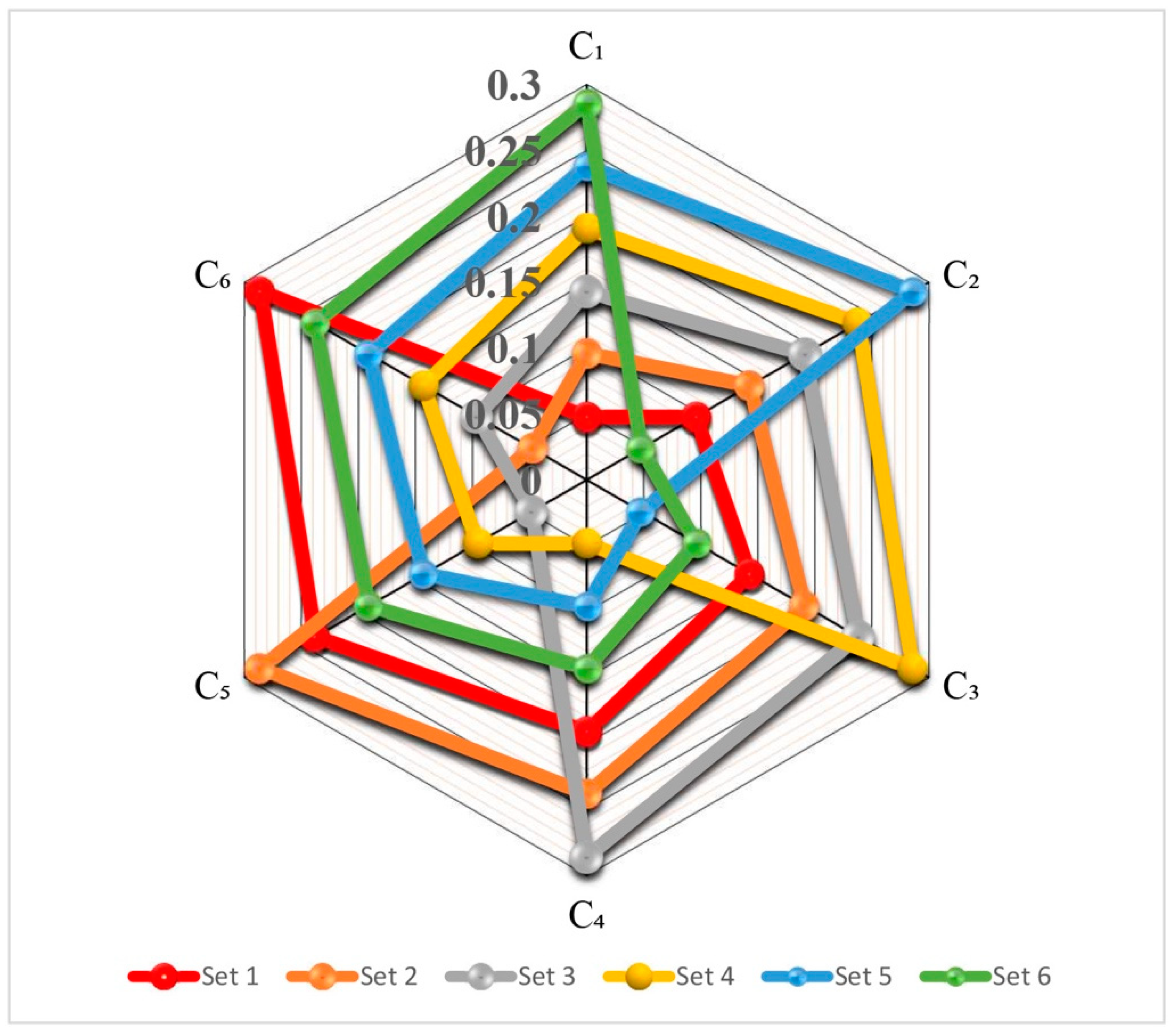
| C1 | C2 | C3 | C4 | C5 | C6 | Order | |
|---|---|---|---|---|---|---|---|
| Set 1 | 0.048 | 0.096 | 0.143 | 0.191 | 0.238 | 0.286 | S(3) S(4) S(1) S(2) |
| Set 2 | 0.096 | 0.143 | 0.191 | 0.238 | 0.286 | 0.048 | S(3) S(4) S(1) S(2) |
| Set 3 | 0.143 | 0.191 | 0.238 | 0.286 | 0.048 | 0.096 | S(3) S(4) S(1) S(2) |
| Set 4 | 0.191 | 0.238 | 0.286 | 0.048 | 0.096 | 0.143 | S(3) S(4) S(1) S(2) |
| Set 5 | 0.238 | 0.286 | 0.048 | 0.096 | 0.143 | 0.191 | S(3) S(4) S(1) S(2) |
| Set 6 | 0.286 | 0.048 | 0.096 | 0.143 | 0.191 | 0.238 | S(3) S(4) S(1) S(2) |
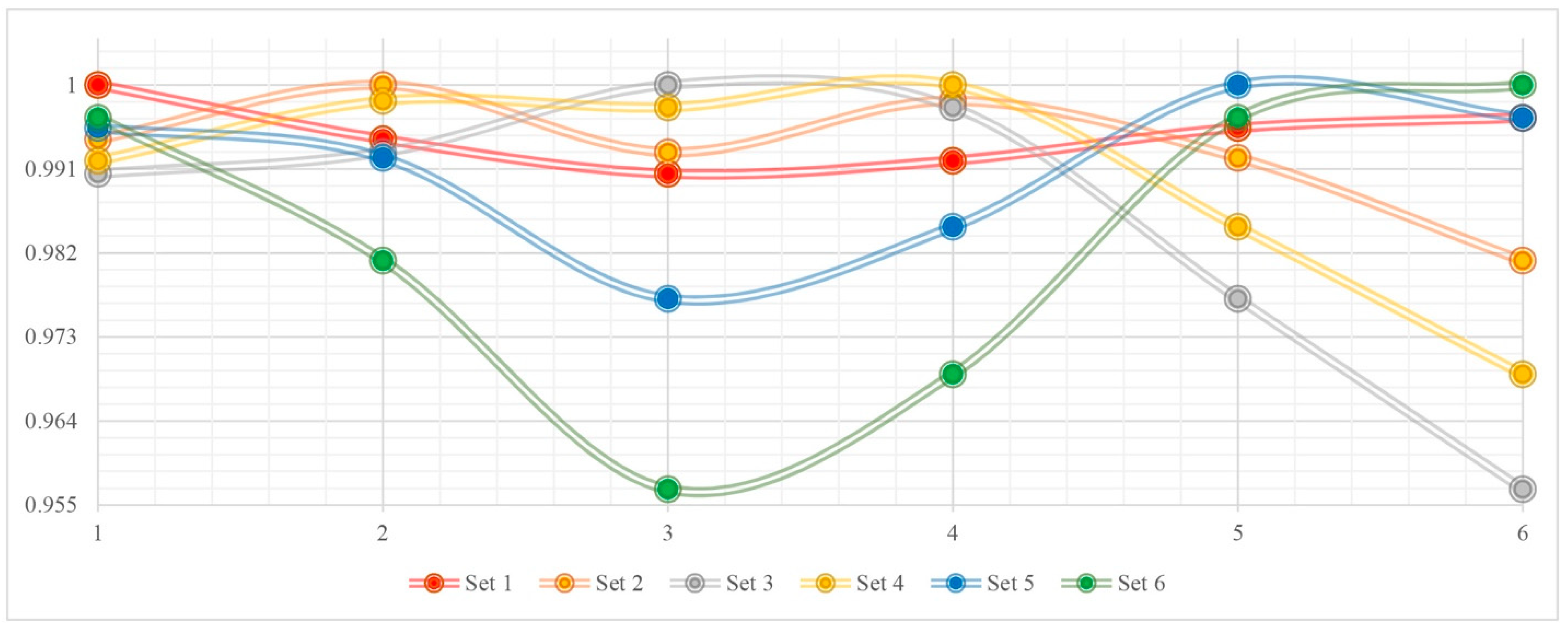
| Set 1 | Set 2 | Set 3 | Set 4 | Set 5 | Set 6 | |
|---|---|---|---|---|---|---|
| Set 1 | 1 | 0.9942 | 0.9905 | 0.9919 | 0.9954 | 0.9965 |
| Set 2 | 0.9942 | 1 | 0.9928 | 0.9983 | 0.9922 | 0.9812 |
| Set 3 | 0.9905 | 0.9928 | 1 | 0.9976 | 0.9771 | 0.9567 |
| Set 4 | 0.9919 | 0.9983 | 0.9976 | 1 | 0.9848 | 0.9690 |
| Set 5 | 0.9954 | 0.9922 | 0.9771 | 0.9848 | 1 | 0.9965 |
| Set 6 | 0.9965 | 0.9812 | 0.9567 | 0.9690 | 0.9965 | 1 |
| Suppliers | PZ-WASPAS | ALP-WASPAS | WASPAS-N | O-WASPAS | Classic WASPAS | |||||
|---|---|---|---|---|---|---|---|---|---|---|
| Order | Order | Order | Order | Order | ||||||
| S(1) | 0.560 | 3 | 0.697 | 3 | 0.775 | 3 | 0.230 | 3 | 0.230 | 3 |
| S(2) | 0.466 | 4 | 0.600 | 4 | 0.700 | 4 | 0.209 | 4 | 0.208 | 4 |
| S(3) | 0.846 | 1 | 0.905 | 1 | 1.000 | 1 | 0.297 | 1 | 0.296 | 1 |
| S(4) | 0.667 | 2 | 0.786 | 2 | 0.882 | 2 | 0.262 | 2 | 0.262 | 2 |
| - | 0.994 | 0.995 | 0.996 | 0.995 | ||||||
Disclaimer/Publisher’s Note: The statements, opinions and data contained in all publications are solely those of the individual author(s) and contributor(s) and not of MDPI and/or the editor(s). MDPI and/or the editor(s) disclaim responsibility for any injury to people or property resulting from any ideas, methods, instructions or products referred to in the content. |
© 2025 by the authors. Licensee MDPI, Basel, Switzerland. This article is an open access article distributed under the terms and conditions of the Creative Commons Attribution (CC BY) license (https://creativecommons.org/licenses/by/4.0/).
Share and Cite
Hashemi-Tabatabaei, M.; Amiri, M.; Keshavarz-Ghorabaee, M. An Expected Value-Based Symmetric–Asymmetric Polygonal Fuzzy Z-MCDM Framework for Sustainable–Smart Supplier Evaluation. Information 2025, 16, 187. https://doi.org/10.3390/info16030187
Hashemi-Tabatabaei M, Amiri M, Keshavarz-Ghorabaee M. An Expected Value-Based Symmetric–Asymmetric Polygonal Fuzzy Z-MCDM Framework for Sustainable–Smart Supplier Evaluation. Information. 2025; 16(3):187. https://doi.org/10.3390/info16030187
Chicago/Turabian StyleHashemi-Tabatabaei, Mohammad, Maghsoud Amiri, and Mehdi Keshavarz-Ghorabaee. 2025. "An Expected Value-Based Symmetric–Asymmetric Polygonal Fuzzy Z-MCDM Framework for Sustainable–Smart Supplier Evaluation" Information 16, no. 3: 187. https://doi.org/10.3390/info16030187
APA StyleHashemi-Tabatabaei, M., Amiri, M., & Keshavarz-Ghorabaee, M. (2025). An Expected Value-Based Symmetric–Asymmetric Polygonal Fuzzy Z-MCDM Framework for Sustainable–Smart Supplier Evaluation. Information, 16(3), 187. https://doi.org/10.3390/info16030187