

Indoor Microclimate Monitoring and Forecasting: Public Sector Building Use Case

 ,
,  ,
,  ,
,  and
and
Abstract
1. Introduction
2. Sensor Network
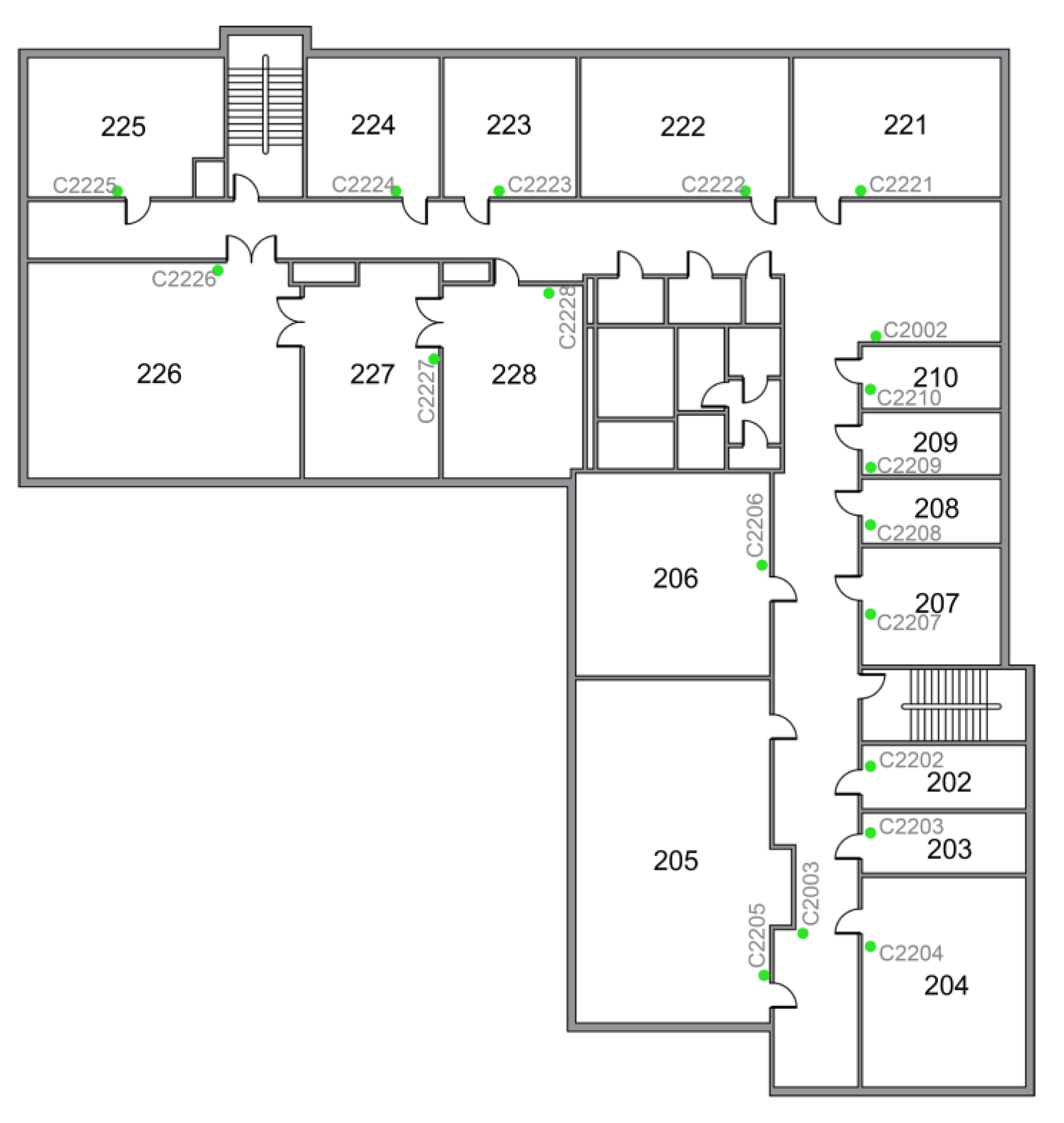
2.1. Description of the Existing IAQ Sensor Network
- —data point count;
- —forecasted value;
- —true value.
- —data point count;
- —forecasted value;
- —true value.
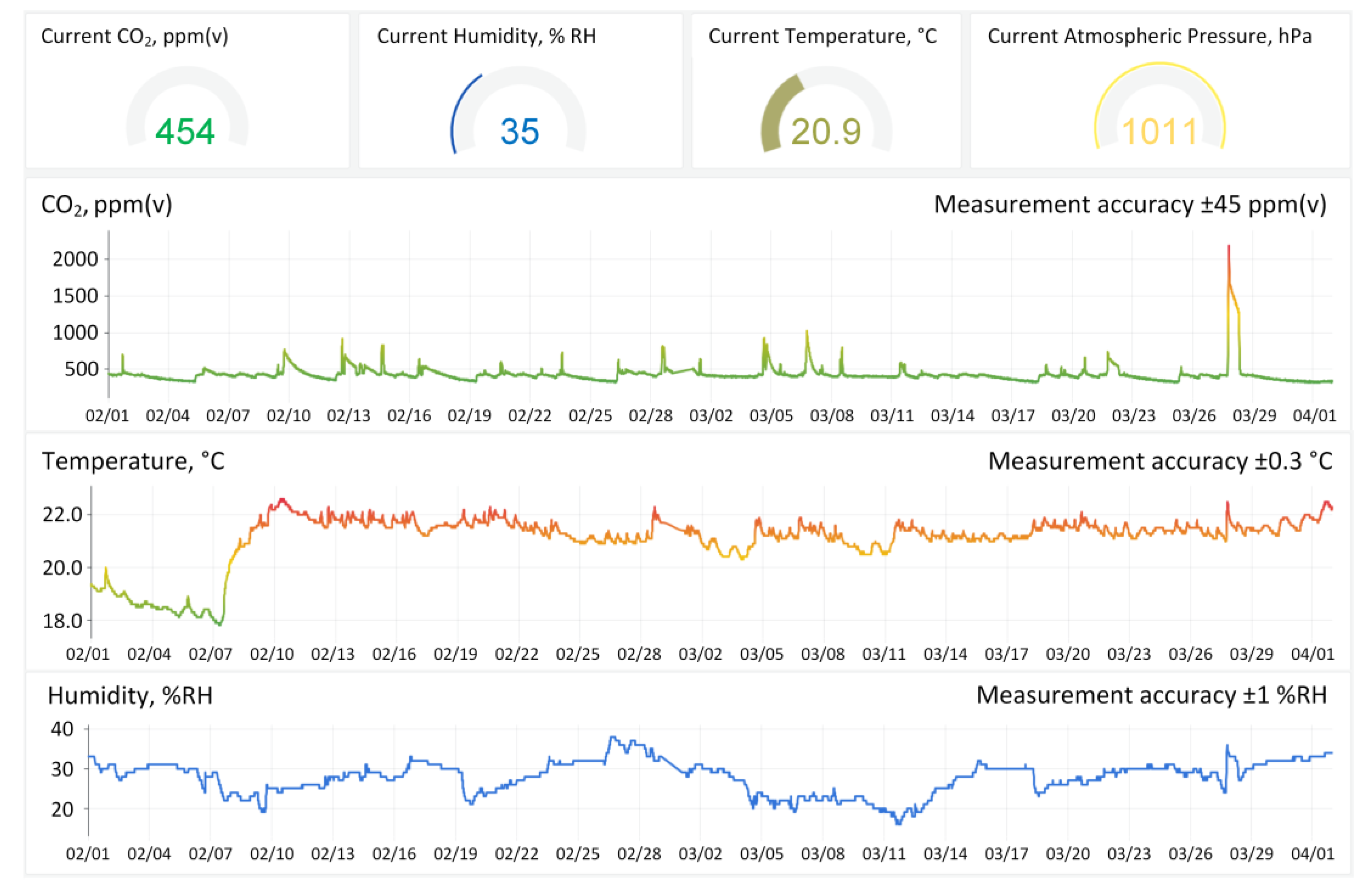
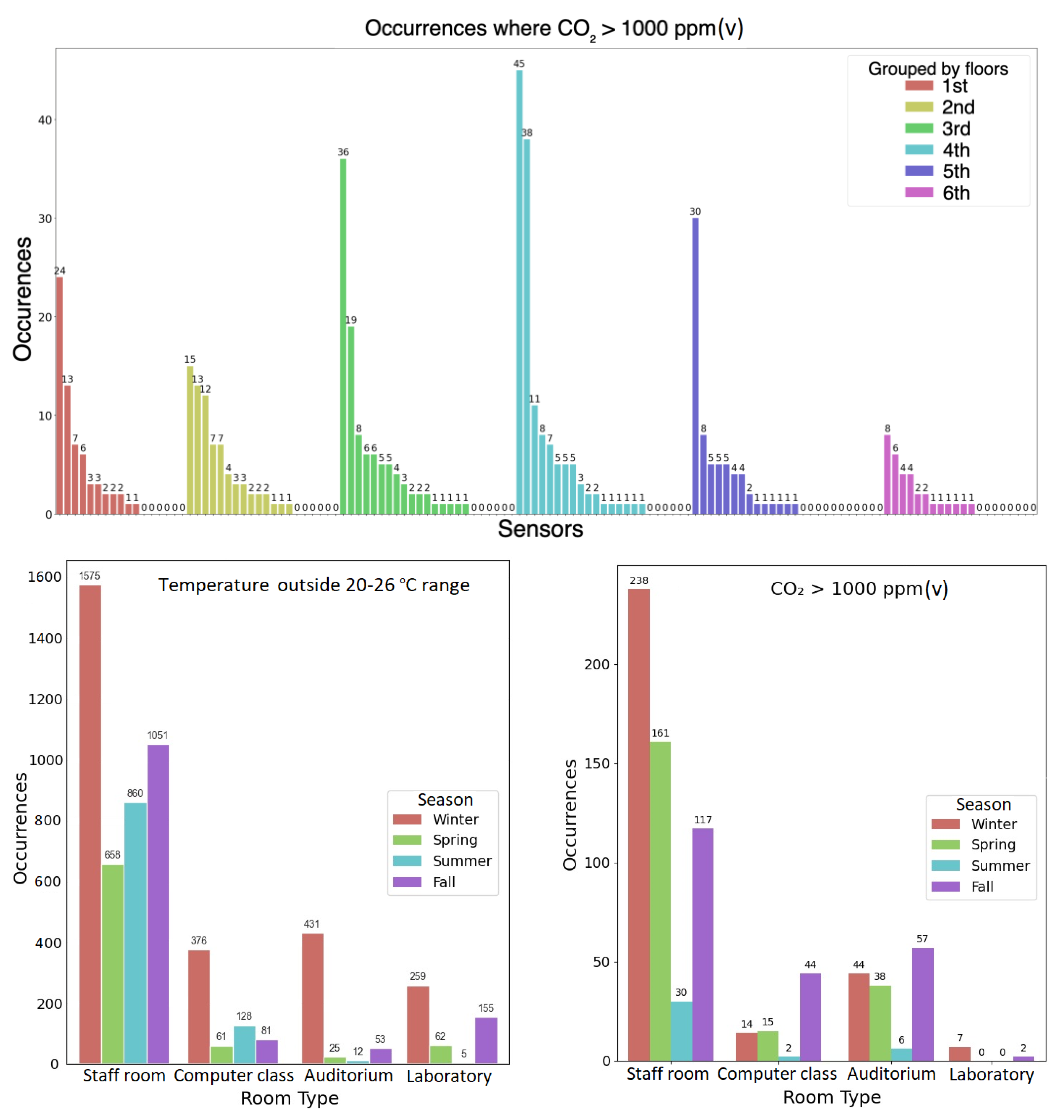
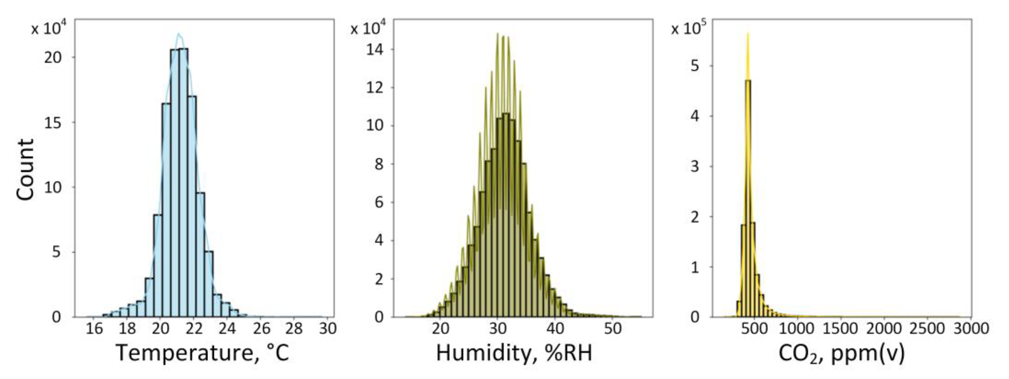
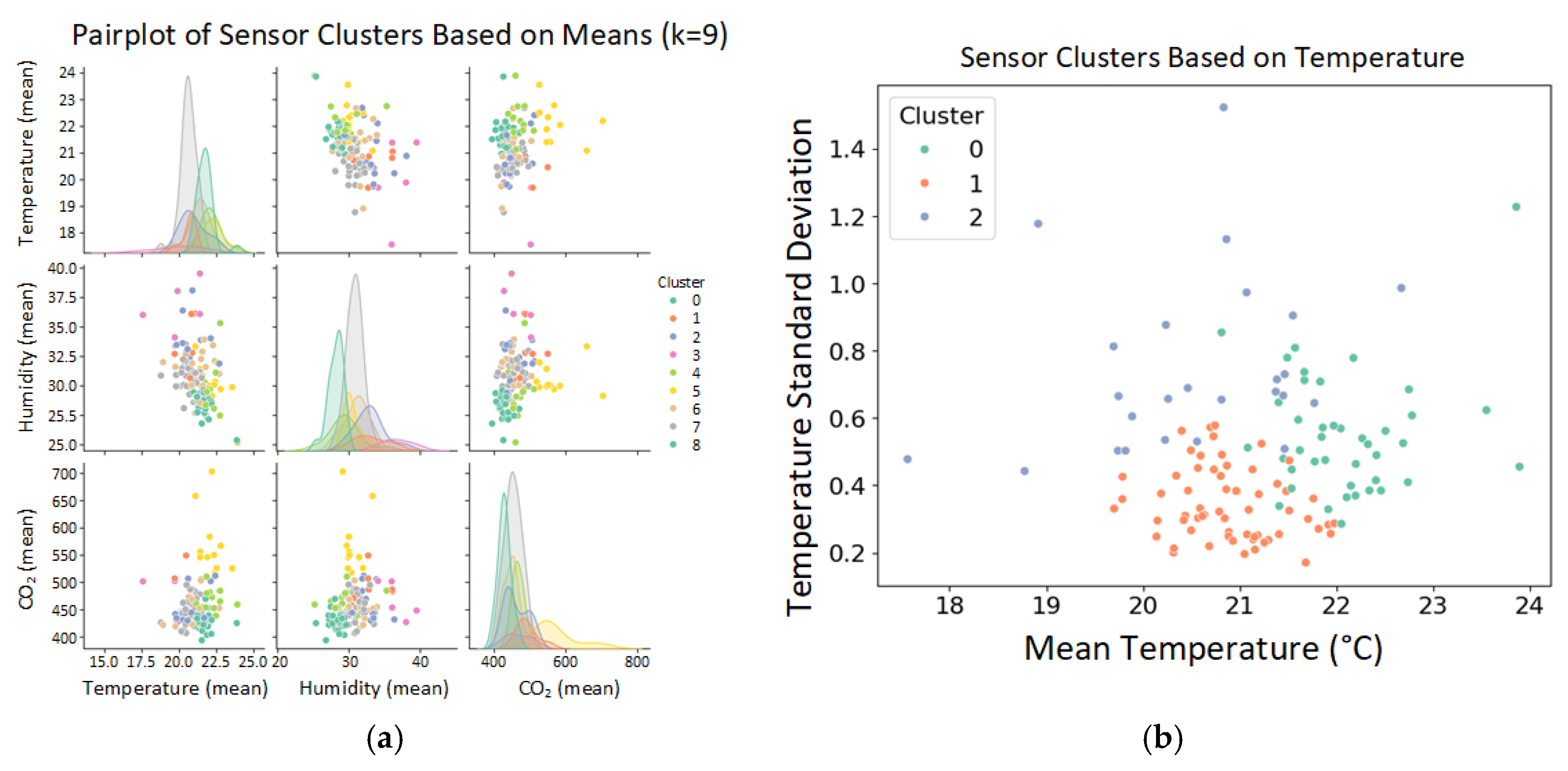
2.2. Analysis of Indoor Air Quality Sensor Datasets
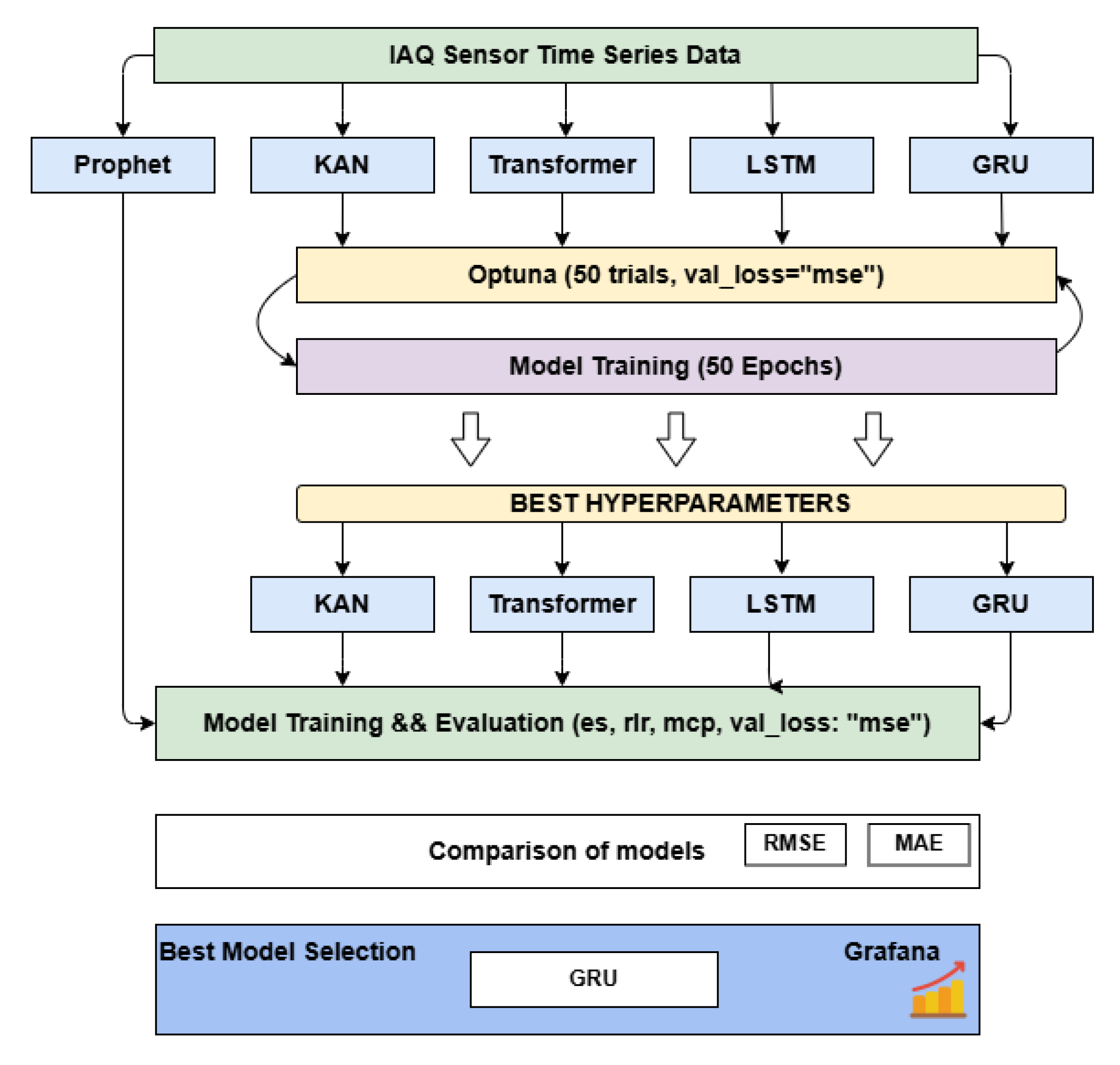
3. Data Forecasting Models
4. Data Prediction Results
4.1. Experiment Description
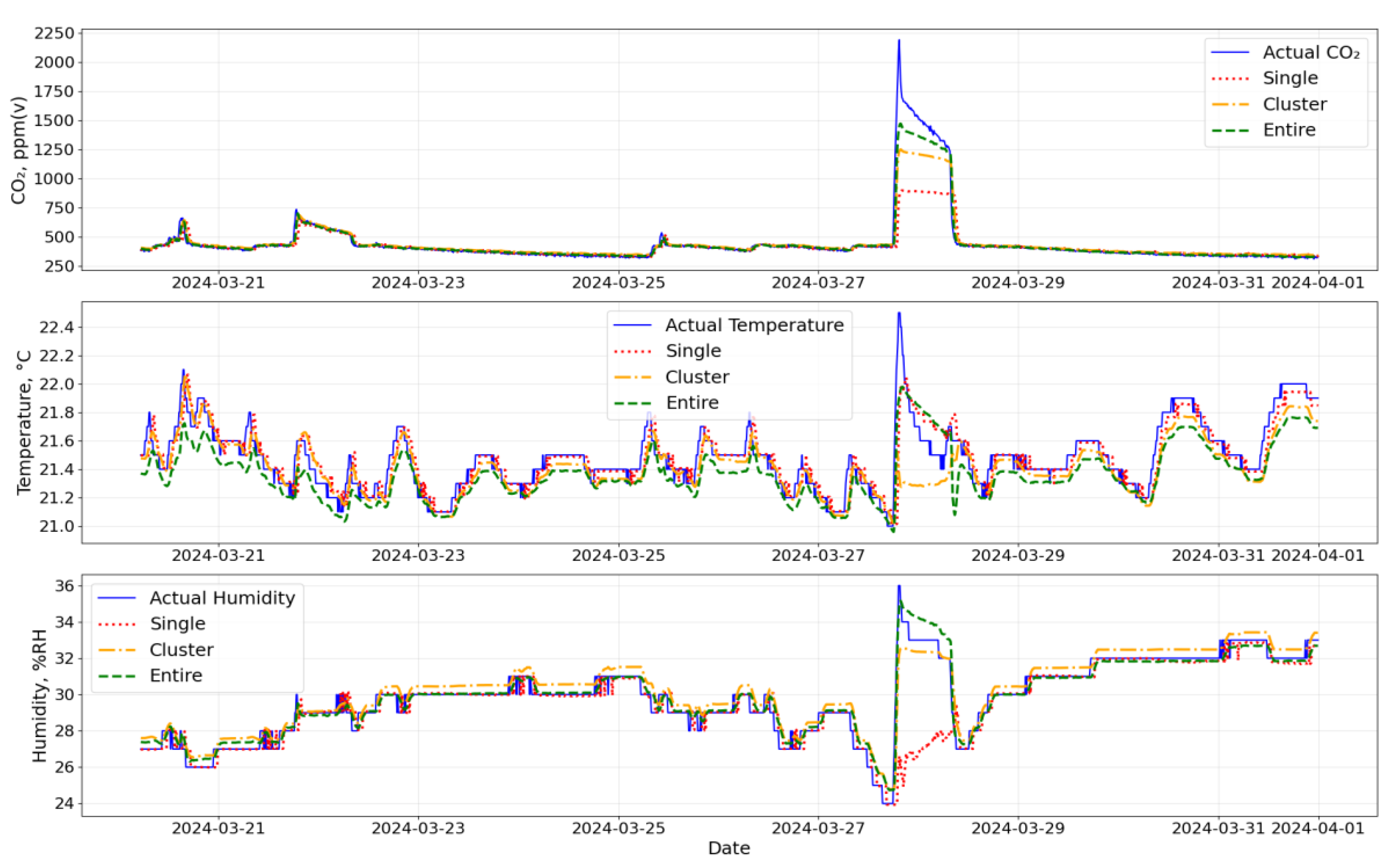
4.2. Data Forecast Using Clusterization Approach
5. Conclusions
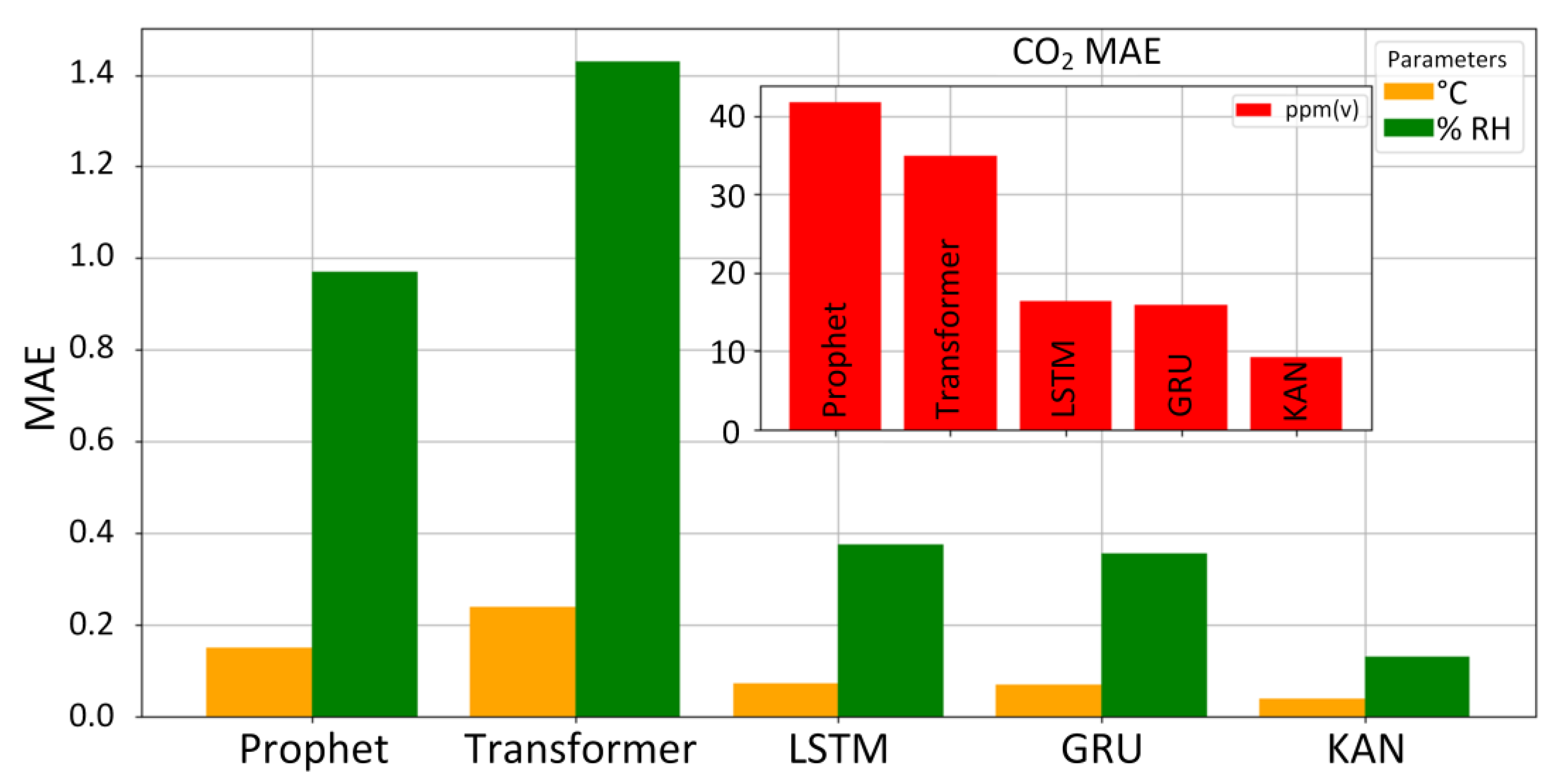
- (1)
- KAN and GRU outperform other models (LSTM, Transformer, and Prophet) regarding prediction accuracy. This is due to the short (2-month) period of IAQ sensor data. It is believed that models like LSTM would perform much better if a longer input data period were used.
- (2)
- GRU is significantly more efficient than the KAN model regarding the computation time (14 min versus 8 h). However, it should be noted that the current KAN model is not optimized for speed.
- (3)
- Clusterization leads to stronger neuron network links, but results in worse MAE and RMSE values.
- (4)
- The LSTM prediction model size for a 2-month period of capturing 128 IAQ sensor data equals 1.164 MB. Creating individual data forecast models for each sensor requires more space (~56 MB) compared to one model for the entire building.
- (5)
- The forecasting system, especially GRU, is scalable and adaptable, making it suitable for application in other public sector buildings with a similar infrastructure.
Author Contributions
Funding
Institutional Review Board Statement
Informed Consent Statement
Data Availability Statement
Conflicts of Interest
Abbreviations
| IAQ | Indoor air quality |
| RMSE | Root Mean Square Error |
| MAE | Mean Absolute Error |
| GRU | Gated Recurrent Unit |
| KAN | Kolmogorov–Arnold Networks |
| ML | Machine Learning |
| HVAC | Heating, Ventilation, and Air Conditioning |
| LSTM | Long Short-Term Memory |
| MLPs | Multi-Layer Perceptrons |
| RNN | Recurrent neural network |
| es | EarlyStopping |
| rlr | ReduceLROnPlateau |
| mcp | ModelCheckpoint |
| mse | Mean Square Error |
| val_loss | Validation loss |
References
- Canha, N.; Correia, C.; Mendez, S.; Gamelas, C.A.; Felizardo, M. Monitoring Indoor Air Quality in Classrooms Using Low-Cost Sensors: Does the Perception of Teachers Match Reality? Atmosphere 2024, 15, 1450. [Google Scholar] [CrossRef]
- Dimitroulopoulou, S.; Dudzińska, M.R.; Gunnarsen, L.; Hägerhed, L.; Maula, H.; Singh, R.; Toyinbo, O.; Haverinen-Shaughnessy, U. Indoor air quality guidelines from across the world: An appraisal considering energy saving, health, productivity, and comfort. Environ. Int. 2023, 178, 108127. [Google Scholar] [CrossRef] [PubMed]
- Palaić, D.; Matetić, I.; Ljubic, S.; Štajduhar, I.; Wolf, I. Data-driven Model for Indoor Temperature Prediction in HVAC-Supported Buildings. In Proceedings of the 2023 3rd International Conference on Electrical, Computer, Communications and Mechatronics Engineering (ICECCME), Tenerife, Spain, 19–21 July 2023; pp. 1–6. [Google Scholar] [CrossRef]
- Saadatifar, S.; Sawyer, A.O.; Byrne, D. Occupant-Centric Digital Twin: A Case Study on Occupant Engagement in Thermal Comfort Decision-Making. Architecture 2024, 4, 390–415. [Google Scholar] [CrossRef]
- Mousavi, Y.; Gharineiat, Z.; Karimi, A.A.; McDougall, K.; Rossi, A.; Gonizzi Barsanti, S. Digital Twin Technology in Built Environment: A Review of Applications, Capabilities and Challenges. Smart Cities 2024, 7, 2594–2615. [Google Scholar] [CrossRef]
- Hauer, M.; Hammes, S.; Zech, P.; Geisler-Moroder, D.; Plörer, D.; Miller, J.; Van Karsbergen, V.; Pfluger, R. Integrating Digital Twins with BIM for Enhanced Building Control Strategies: A Systematic Literature Review Focusing on Daylight and Artificial Lighting Systems. Buildings 2024, 14, 805. [Google Scholar] [CrossRef]
- Qian, Y.; Leng, J.; Zhou, K.; Liu, Y. How to measure and control indoor air quality based on intelligent digital twin platforms: A case study in China. Build. Environ. 2024, 253, 111349. [Google Scholar] [CrossRef]
- Fuller, A.; Fan, Z.; Day, C.; Barlow, C. Digital Twin: Enabling Technologies, Challenges and Open Research. IEEE Access 2020, 8, 108952–108971. [Google Scholar] [CrossRef]
- Saini, J.; Dutta, M.; Marques, G. Machine Learning for Indoor Air Quality Assessment: A Systematic Review and Analysis. Environ. Model. Assess. 2024, 1–8. [Google Scholar] [CrossRef]
- Aranet. User Guide Aranet4 HOME/Aranet4 PRO. Available online: https://aranet.com/attachment/273/Aranet4_User_Manual_v24_WEB.pdf (accessed on 27 December 2024).
- Aranet4 HOME. Available online: https://aranet.com/en/home/products/aranet4-home/ (accessed on 27 December 2024).
- Aranet. Aranet Radio benefits, Aranet Radio vs. LoRaWAN. 8 November 2022. Available online: https://pro.aranet.com/uploads/2022/11/aranet_radio_vs_lorawan_v4.pdf (accessed on 27 December 2024).
- Arturs Ziemelis, Ruslans Sudniks, and Andis Supe, VPP Mote [Data set]. Kaggle. 2024. [CrossRef]
- Scikit-Learn. Metrics and Scoring: Quantifying the Quality of Predictions. Available online: https://scikit-learn.org/stable/modules/model_evaluation.html#mean-absolute-error (accessed on 20 December 2024).
- Scikit-Learn. Root_Mean_Squared_Error. Available online: https://scikit-learn.org/stable/modules/generated/sklearn.metrics.root_mean_squared_error.html (accessed on 20 December 2024).
- Archive of Air Temperature and Wind Speed Data. Available online: https://www.meteolapa.lv/arhivs/1217/riga/01-02-2024/31-03-2024 (accessed on 18 December 2024).
- Sudniks, R.; Ziemelis, A.; Spolitis, S.; Nikitenko, A.; Supe, A. Development of Building Indoor Air Quality Monitoring Based on IoT Sensor Network. In Proceedings of the 2024 Photonics & Electromagnetics Research Symposium (PIERS), Chengdu, China, 21–25 April 2024; IEEE: Piscataway, NJ, USA, 2024; pp. 1–7. [Google Scholar] [CrossRef]
- KindXiaoming. KAN GitHub. Available online: https://github.com/KindXiaoming/pykan (accessed on 13 November 2024).
- Popescu, M.-C.; Balas, V.; Perescu-Popescu, L.; Mastorakis, N. Multilayer perceptron and neural networks. WSEAS Trans. Circuits Syst. 2009, 8, 579–588. [Google Scholar]
- Taylor, S.J.; Letham, B. Forecasting at scale. PeerJ Prepr. 2017, 5, e3190v2. [Google Scholar] [CrossRef]
- Liu, K.; Zhang, J. A Dual-Layer Attention-Based LSTM Network for Fed-batch Fermentation Process Modelling. In Computer Aided Chemical Engineering; Elsevier: Amsterdam, The Netherlands, 2021; Volume 50, pp. 541–547. ISBN 978-0-323-88506-5. [Google Scholar]
- Ebrahimi, Z.; Loni, M.; Daneshtalab, M.; Gharehbaghi, A. A review on deep learning methods for ECG arrhythmia classification. Expert Syst. Appl. X 2020, 7, 100033. [Google Scholar] [CrossRef]
- Vaswani, A.; Shazeer, N.; Parmar, N.; Uszkoreit, J.; Jones, L.; Gomez, A.N.; Kaiser, L.; Polosukhin, I. Attention Is All You Need. arXiv 2023, arXiv:1706.03762. [Google Scholar]
- Akiba, T.; Sano, S.; Yanase, T.; Ohta, T.; Koyama, M. Optuna: A Next-generation Hyperparameter Optimization Framework. In Proceedings of the 25th ACM SIGKDD International Conference on Knowledge Discovery & Data Mining, Anchorage, AK, USA, 4–8 August 2019; ACM: New York, NJ, USA, 2019; pp. 2623–2631. [Google Scholar] [CrossRef]
- KMeans. Available online: https://scikit-learn.org/stable/modules/generated/sklearn.cluster.KMeans.html (accessed on 18 December 2024).


| Parameter | GRU | LSTM | Transformer | KAN |
|---|---|---|---|---|
| Optuna | 50 trials | 50 trials | 50 trials | 50 trials |
| epochs/steps | 50 epochs | 50 epochs | 50 epochs | 20 steps |
| num_units/heads | 256 neurons | 192 neurons | 2 heads | hidden dim = 12 |
| num_layers | 1 | 1 | 8 | N/A |
| ff_dim | N/A | N/A | 96 | grid = 7 |
| dropout_rate | 0.1 | 0.2 | 0.1 | N/A |
| recurrent_dropout | 0.2 | 0 | N/A | N/A |
| learning_rate | ~0.0008965 | ~0.000128 | ~0.00059 | ~0.003544 |
| batch_size | 32 | 32 | 96 | N/A |
| optimizer | adam | adam | adam | LBFGS |
| bidirectional | True | True | N/A | N/A |
| additional params | N/A | N/A | N/A | k = 3, lamb = 0.000622 |
| Model | Feature | RMSE | MAE | Computation Time | ||||
|---|---|---|---|---|---|---|---|---|
| Min | Max | Mean | Min | Max | Mean | |||
| Prophet | Temp | 0.07 | 0.45 | 0.21 | 0.06 | 0.34 | 0.15 | 18 min |
| CO2 | 10.39 | 287.03 | 64.13 | 7.95 | 219.47 | 41.62 | ||
| RH | 0.76 | 2.65 | 1.34 | 0.56 | 2.12 | 1.02 | ||
| LSTM | Temp | 0.05 | 0.34 | 0.11 | 0.03 | 0.19 | 0.07 | 17 min |
| CO2 | 8.35 | 226.46 | 30.04 | 6.34 | 78.96 | 16.36 | ||
| RH | 0.37 | 1.83 | 0.62 | 0.17 | 0.83 | 0.38 | ||
| Transformer | Temp | 0.06 | 0.87 | 0.31 | 0.04 | 0.74 | 0.24 | 51 min |
| CO2 | 11.76 | 202.89 | 48.15 | 9.35 | 129.45 | 34.87 | ||
| RH | 0.49 | 5.21 | 1.79 | 0.33 | 4.55 | 1.43 | ||
| KAN | Temp | 0.03 | 0.61 | 0.07 | 0.02 | 0.19 | 0.04 | 506 min |
| CO2 | 6.39 | 37.37 | 15.00 | 4.88 | 17.27 | 9.20 | ||
| RH | 0.19 | 0.89 | 0.27 | 0.08 | 0.37 | 0.13 | ||
| GRU | Temp | 0.05 | 0.34 | 0.11 | 0.03 | 0.19 | 0.07 | 14 min |
| CO2 | 8.61 | 223.07 | 29.74 | 6.36 | 77.75 | 15.96 | ||
| RH | 0.36 | 1.75 | 0.61 | 0.15 | 0.74 | 0.36 | ||
| Model | Cluster | Temperature | CO2 | Humidity | Model Size, kBytes | |||
|---|---|---|---|---|---|---|---|---|
| RMSE | MAE | RMSE | MAE | RMSE | MAE | |||
| LSTM | Entire Dataset | 0.29 | 0.24 | 46.30 | 26.97 | 1.04 | 0.77 | 1164 |
| cluster 0 | 0.16 | 0.12 | 35.80 | 25.40 | 0.70 | 0.53 | 915 | |
| cluster 1 | 0.19 | 0.15 | 43.27 | 22.83 | 1.03 | 0.77 | 960 | |
| cluster 2 | 0.26 | 0.20 | 40.50 | 23.53 | 1.11 | 0.82 | 849 | |
| Transformer | Entire Dataset | 0.31 | 0.24 | 47.52 | 33.2 | 1.12 | 0.83 | 7025 |
| cluster 0 | 0.38 | 0.34 | 51.03 | 32.63 | 1.56 | 1.29 | 1151 | |
| cluster 1 | 0.22 | 0.15 | 45.36 | 26.72 | 1.14 | 0.88 | 1830 | |
| cluster 2 | 0.56 | 0.45 | 57.35 | 31.087 | 2.04 | 1.53 | 1260 | |
| GRU | Entire Dataset | 0.16 | 0.12 | 28.51 | 17.97 | 0.75 | 0.57 | 890 |
| cluster 0 | 0.16 | 0.11 | 43.28 | 28.07 | 0.65 | 0.41 | 703 | |
| cluster 1 | 0.13 | 0.09 | 32.91 | 12.60 | 0.71 | 0.46 | 737 | |
| cluster 2 | 0.19 | 0.14 | 32.92 | 14.77 | 0.86 | 0.63 | 653 | |
Disclaimer/Publisher’s Note: The statements, opinions and data contained in all publications are solely those of the individual author(s) and contributor(s) and not of MDPI and/or the editor(s). MDPI and/or the editor(s) disclaim responsibility for any injury to people or property resulting from any ideas, methods, instructions or products referred to in the content. |
© 2025 by the authors. Licensee MDPI, Basel, Switzerland. This article is an open access article distributed under the terms and conditions of the Creative Commons Attribution (CC BY) license (https://creativecommons.org/licenses/by/4.0/).
Share and Cite
Sudniks, R.; Ziemelis, A.; Nikitenko, A.; Soares, V.N.G.J.; Supe, A. Indoor Microclimate Monitoring and Forecasting: Public Sector Building Use Case. Information 2025, 16, 121. https://doi.org/10.3390/info16020121
Sudniks R, Ziemelis A, Nikitenko A, Soares VNGJ, Supe A. Indoor Microclimate Monitoring and Forecasting: Public Sector Building Use Case. Information. 2025; 16(2):121. https://doi.org/10.3390/info16020121
Chicago/Turabian StyleSudniks, Ruslans, Arturs Ziemelis, Agris Nikitenko, Vasco N. G. J. Soares, and Andis Supe. 2025. "Indoor Microclimate Monitoring and Forecasting: Public Sector Building Use Case" Information 16, no. 2: 121. https://doi.org/10.3390/info16020121
APA StyleSudniks, R., Ziemelis, A., Nikitenko, A., Soares, V. N. G. J., & Supe, A. (2025). Indoor Microclimate Monitoring and Forecasting: Public Sector Building Use Case. Information, 16(2), 121. https://doi.org/10.3390/info16020121