Performance Improvement of Vehicle and Human Localization and Classification by YOLO Family Networks in Noisy UAV Images

Abstract

Many important tasks in smart city development and management are solved by systems of monitoring and control installed on-board of unmanned aerial vehicles (UAVs). UAV sensors can be imperfect or they can operate in unfavorable conditions, which can then result in obtaining images or video sequences that are noisy. Noise can degrade the performance of methods of vehicle and human localization and classification. Therefore, specific techniques to improve performance have to be applied. In this paper, we consider YOLO family neural networks as tools for solving the aforementioned tasks. This family of networks is rapidly developing; however, the input data may still require pre-processing. One option is to apply denoising before object localization and classification. In addition, approaches based on augmentation and training can be used as well. We consider the performance of these approaches for various noise intensities. We identify the noise levels at which network performance starts to degrade and analyze possibilities of performance improvement for two filters–BM3D and DRUNet. Both improve such performance criteria as the F1 score, the Intersection over Union and the mean Average Precision. Datasets of urban areas are used in the network training and verification.

1. Introduction

The theory and practice of smart cities have become of high interest to researchers, companies and local authorities [1,2]. These theories and practices unite such modern technologies as the Internet of Things, artificial intelligence, drones [3] and so on. There are numerous particular applications of these technologies, especially of drones and unmanned aerial vehicles (UAVs), such as for traffic control [4,5], detection and classification of moving objects [6], including pedestrians at a distance [7], crowd-counting [8], tree and streetlight control [9], etc.

All aforementioned applications are (to different degrees) based on object detection, localization and classification from drones and UAVs [10] using digital cameras and means of intellectual image/video processing, mainly employing pre-trained convolutional neural networks (CNNs) [11,12,13,14,15]. Despite the development of CNNs (appearance of new types of CNNs, new achievements in their training, increase in data processing speed and decrease in power consumption), there are still various problems preventing their wider application for the considered (smart cities) and other applications [15,16,17,18]. One problem can be the quality of original images or videos due to bad weather conditions, noise, blur and other reasons [17,18]. These factors result in worse localization and classification, a decrease in tracking and control performance, etc. Another problem is localization and classification of small and closely placed objects [15,19,20]. One more problem is the choice of a proper CNN since it is always a compromise between efficiency, computational load, power consumption, etc. Note that many types of CNNs have already been shown to be efficient in object localization and classification, including Faster R-CNN [13], RetinaNet [21], Single Shot Detector (SSD) [14] and You Only Look Once (YOLO) [18,19,22]. Finally, to train a CNN, one needs a properly marked dataset containing objects of the classes of interest [23,24].

Our recent papers [15,25] consider the performance of several CNNs in conditions of additive white Gaussian noise presence. In [25], the study is carried out for Faster Recurrent Convolution Neural Network (Faster R-CNN) [13], RetinaNet [21], Single Shot Detector (SSD) [14] and two versions of YOLO, namely YOLOv5 [22] and YOLOv8 [26]. It is shown that, according to the F1 score [27] and Intersection of Union (IoU) [28], the best performance for noise-free images is provided by both versions of YOLO CNNs. However, for intensive noise, performance of all considered CNNs becomes worse according to both aforementioned criteria where YOLOv8 is less sensitive to noise than other CNNs. Note that all CNNs have been trained using noise-free images.

The paper [15] analyzes performance for eleven CNNs, namely, four versions of Faster R-CNN (ResNet18, ResNet50, ResNet101 and ResNetXt [29]), four versions of Retina Net (ResNet18, ResNet50, ResNet101 and ResNetXt), two versions of SSD (MobileNetV2 [30] and VGG16 [31]) and YOLOv5m. SSD and YOLO CNNs demonstrated good performance for noise-free images according to the F1 score, but the presence of noise led to significant degradation of the F1 score. Other considered metrics, IoU and percentage of correctly predicted regions (PoCPR), have been less influenced by noise. A specific feature of the paper [25] consists of an analysis to improve performance characteristics of CNNs through image pre-filtering by the color version of the block matching three-dimensional (BM3D) filter [32,33] and the DRUNet NN-based filter [34]. When proposing the application of pre-filtering, we kept in mind that such pre-processing was helpful in analogous practical situations using UAV-based images in noisy environments [35,36,37].

Other important conclusions of the papers [15,25] include the following: (a) the considered versions of YOLO CNNs are able to provide rather good results; (b) pre-filtering can be useful, especially if the NN-based DRUNet filter is applied; (c) one should carefully choose datasets for training and verification since non-careful markup can lead to biased estimates of IoU; (d) pre-filtering might take approximately the same time as localization and classification; (e) small-sized objects containing less than 200 pixels are localized and classified worse than objects of a larger size, and image pre-filtering for small-sized objects is less beneficial than for larger-sized objects.

Meanwhile, several questions have not been answered. First, are other versions of YOLO family networks able to provide better results than YOLOv5 and YOLOv8? Note that the YOLO family of CNNs develops quickly [38,39]. We should also stress that new versions of YOLO demonstrate very good performance for several applications. For example, an improved YOLOv7 model has been recently applied to low-quality UAV images to detect surface damage on wind turbine blades [40]. A YOLO-SMUG version has been proposed for efficient and lightweight object detection using infrared sensors [41]. For a similar application, a YOLO-UIR version has been proposed [19]. A YOLO-UAV version has been designed and applied to object detection in UAV-based imagery based on multi-scale feature fusion [42].

Another question is the following—can the CNN performance be improved by augmentation [43], in particular, by injecting noise into images exploited in training [44,45]? Since both preliminary denoising and training with augmentation can lead to positive outcomes, then what approach is preferable and why?

Thus, the main novelty and contributions of the paper consist in the following:

(1)

We have analyzed the performance of six versions of YOLO CNNs (namely, nano and medium versions of YOLOv5, YOLOv8 and YOLOv11) for noise-free and noisy color images contaminated by additive white Gaussian noise (AWGN) and established noise levels that start to lead to significant negative outcomes according to four traditional criteria used in the practice of performance analysis for methods of object localization and classification.

(2)

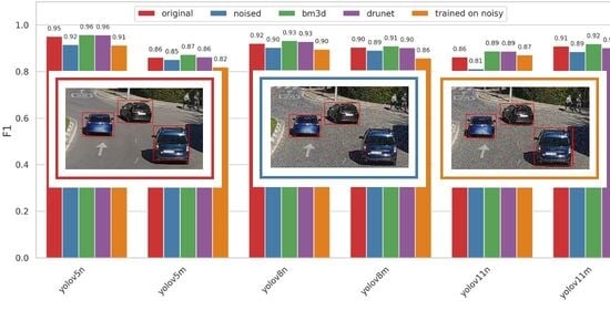
Possibilities of performance improvement by image pre-filtering using traditional and neural network-based filters have been analyzed and shown to be efficient for high noise levels.

(3)

Possibilities of using augmentation by noise injection at the stage of CNN training have been studied as well; performance of this approach has been compared to performance of image processing with pre-filtering; it is demonstrated that the approach based on denoising produces slightly better results.

(4)

CNN performance has been validated for new datasets (including the TAI dataset with better annotation quality); the IoU-related conclusions have been re-evaluated and become more adequate.

(5)

The influence of the object size on localization and classification characteristics has been briefly studied.

(6)

The case of Poisson noise has been investigated as well; it is shown that the obtained tendencies and results are in good agreement with the case of AWGN.

Compared to our earlier papers [15,25], here we consider more versions of YOLO family CNNs, including YOLOv11, analyze more datasets, study the cases of small-sized objects and CNN learning with noise injection, investigate images contaminated by Poisson noise and employ mean Average Precision (mAP) in addition to previously used metrics.

The structure of the paper is the following. The methodology of the study and image/noise model are introduced and briefly considered in Section 2. Peculiarities of CNN training and performance criteria are given in Section 3. Performance of pre-filtering and outcomes of its use are analyzed in Section 4. The effectiveness of augmentation via noise injection is discussed in Section 5. The results for Poisson noise, some aspects of computational load and discussion are given in Section 6. Finally, the conclusions and directions of future work are presented.

2. Image/Noise Model and Methodology

In general, drone- and UAV-based sensors can produce various types of images, including optical, infrared and radar [46]. Below we deal with color images or frames of color video, which are, probably, the most typical. Due to limitations on weight and power consumption, sensors installed on UAVs and drones usually produce images of a size significantly smaller than customer digital cameras. Then, the acquired images usually have several hundred × several hundred pixels [47]. This is also related to the fact that the CNNs that perform the object localization and classification operate with data arrays of fixed and even smaller sizes.

2.1. Methodology of Our Study

It is clear that the performance of methods and tools of object localization and classification for noise-free and noisy images depends on several factors, namely, the following:

-

The considered CNN and its basic characteristics;

-

The CNN training approach used and properties of a dataset or datasets employed for training and verification;

-

Image quality (types of degradations and their characteristics);

-

Methods and algorithms of image pre-processing (if applied).

Certainly, one also has to choose the adequate criteria of data processing efficiency.

We have already mentioned that our main focus are YOLO family CNNs [38,39]. Note that the CNN architecture must meet the system requirements in terms of accuracy, computational complexity and power. Keeping this in mind, we have chosen YOLO CNNs of different generations and versions. In total, we study the 5th generation (YOLOv5) [22], 8th generation (YOLOv8) [26] and 11th generation (YOLOv11) [48]. As modifications, we have chosen the nano version, which corresponds to the smallest version with a low computational load, allowing it to be used on portable devices (UAVs), but it also has the lowest accuracy rates. We have also chosen the medium version, which is claimed to be a compromise between accuracy and computational load [22]. The general list of neural networks under study is as follows: YOLOv5n (nano), YOLOv5m (medium), YOLOv8n, YOLOv8m, YOLOv11n and YOLOv11m.

To study the performance of modern methods of image processing in general, and object localization and classification in particular, one usually needs a set of images of different complexities. Since our focus is on methods presuming CNN training, we have to employ datasets containing thousands of images. The set or sets used for validation should contain many images, too. The used datasets are described in Section 3.1.

Acquired images of video frames can be of different quality due to several factors, such as weather conditions (e.g., fog [49] and rain [50]), noise of various types [35,36,37], blur [51] and effects of lossy compression [52]. Depending upon the situation at hand, different factors can be dominant and may possibly have a joint negative influence. In this paper, we focus on studying the influence of the noise and ways to cope with this phenomenon since noise alone is often the dominant factor.

We mainly rely on the model of AWGN in all components of the original color image. We clearly understand that this model has limitations and, for particular cases, noise can be signal-dependent, spatially correlated or both [33,53,54]. Our decision to employ the AWGN model has been motivated by the following. First, AWGN is the simplest model used most often and especially as a starting point in studies dealing with noise influence or noisy image processing [54,55,56]. Second, in our earlier paper [15], we used the AWGN model as well. So, the results obtained and described in the current paper can be compared to the results from the paper [15]. Third, if the noise is signal-dependent or spatially correlated, one has an infinity of options for setting and varying its parameters. Note that each individual sensor installed on a UAV or drone or a digital camera might have its own noise characteristics [57]. Fourth, if characteristics of a signal-dependent noise are a priori known or pre-estimated with high accuracy [57], it is possible to perform the corresponding variance stabilizing transform (VST), converting an image corrupted by signal-dependent noise to an image contaminated by additive (although not always Gaussian) noise with practically constant variance [33,53]. Recall that there is a considerably larger amount of good filters [58] able to efficiently remove AWGN signal-dependent noise.

Meanwhile, we have also considered the Poisson noise model as an alternative to the AWGN model. The obtained results are presented in Section 6.1.

Finally, it is possible to apply some pre-processing of data [25] and/or to take into account possible noise presence in images at the CNN training stage. To the best of our knowledge, no thorough analysis of what is better exists. Because of this, our particular task is to compare the corresponding approaches.

Thus, relying on traditional criteria for object localization and classification (see Section 3.2), we perform the following:

-

Carry out training for all six CNN versions for both noise-free images and noisy one obtained via noise injection (see Section 5 for more details);

-

Perform noisy image pre-filtering assuming noise type and characteristics are known in advance (see Section 4.2 and Section 6.1 for more details);

-

Calculate the used quantitative criteria for all six CNNs for each noise intensity for noisy images, for images processed by all considered filters, and for the case of CNN training via noise injection;

-

Analyze and compare the performance for all aforementioned variants of CNNs, their training and filters applied to obtain conclusions and recommendations;

-

In addition, we pay attention to particular aspects of CNN realization on-board, keeping in mind possible practical limitations.

2.2. Basic Noise Model

As said above, at the beginning we assume that images are given in RGB format and the noise is AWGN, having zero mean and variance σ² or standard deviation (STD) σ and that that is the same in all three color components. The noise realizations are assumed to be independent (uncorrelated to each other) in component images. Then one has

$$I_{k ij}^n=I_{k ij}^t+n_{k ij}.$$

(1)

In (1), $I_{k ij}^n$ denotes the noisy image value in the ij-th pixel of the k-th component (k = 1, …, 3), $I_{k ij}^t$ is the corresponding true value and $n_{k ij}$ denotes noise in the ij-th pixel in the k-th component image with $n_{k ij}\sim \mathcal{N}\left(0, \sigma ²\right)$.

Consider the possible range of STD variations to be studied. The results presented in [15,25] show that noise with a STD smaller than 5 rarely has a noticeable negative impact on object localization and classification. In other words, the presence of invisible noise (recall that AWGN can be noticeable for STD ≈ 5 in color images of simple complexity and for larger STDs in textural images and mainly in quasi-homogeneous image regions) has practically no negative outcomes.

To simulate visible noise, STD values equal to 7, 10, 15, 20 and 25 have also been considered. This corresponds to the peak signal-to-noise ratio (PSNR, $PSNR=10lo{g}_{10}\left({\displaystyle \frac{{255}^2}{{\sigma }^2}}\right)$) in the limits below 31 dB (input PSNR = 20.3 dB in the most complex case of STD = 25). An input PSNR of about 20 dB rarely occurs in practice, but it can be treated as an extreme case. Choosing the aforementioned STD and PSNR values, we have taken into account that digital cameras might work in different illumination conditions. Experiments carried out for real-world situations for different digital cameras [59,60,61,62] show that an input PSNR of less than 30 and even of 25 dB is quite probable in practice. Moreover, there have been attempts to simulate realistic noise [63,64]. Meanwhile, although many papers concerning CNN-based denoising (e.g., [34]) consider in their simulations a STD = 50 (PSNR about 15 dB), such an STD value is, in our opinion, unrealistic.

The cases in which the noise STD is equal to 5 and 15 are illustrated in Figure 1. As can be seen, the noise of STD = 5 is hardly noticeable in the images in Figure 1a,c, whilst the noise of STD = 15 is clearly visible (Figure 1b,d). Moreover, intensive noise influences the classification of humans (as smaller sized objects) more than the classification of cars which usually have a larger number of pixels corresponding to them [15].

Information about the datasets used in training and validation will be given later.

3. CNN Training, Performance Criteria for Object Localization and Classification and Preliminary Results

3.1. Used Datasets, Considered CNNs and Their Training

Selecting a dataset for training of a neural network is one of the main tasks that needs to be accomplished, because the accuracy of the neural network and its ability to recognize certain types of objects depend on the dataset. Important factors in choosing a dataset are its size (number of images and number of labeled regions), the quality of labeling, the number of classes (and coverage of the necessary classes) and the variability of images. One such dataset that covers the necessary characteristics for our research is VisDrone [24]. Its training part contains 6471 images with high variability, in which 369,595 regions distributed into 10 classes are labeled. The largest classes in terms of the number of regions are “Cars”, with 152,469 regions, accounting for 41.2% of the total number of regions, and the “Humans” class, with 120,505 regions, accounting for 32.6% of the total number of regions.

Neural network training was conducted in a modified infrastructure from ultralytics [22], which we have adapted to our needs. During training, we used standard pa-rameters for each of the neural networks under study, but with the Early Stopping algo-rithm to prevent overfitting. Based on the data obtained during training, we can plot the changes in the mAP0.5:0.95 metric, which is responsible for the accuracy of the model, as shown in Figure 2.

There is a noticeable similarity in behavior for most neural networks, which are visually divided into “clusters”—these are nano versions (the values for YOLOv8n and YOLOv11n are almost identical) and medium versions (the values for YOLOv11m is the best). This behavior indicates the similarity of neural networks between generations and, of course, the difference in accuracy between the nano and medium modifications of the CNNs.

3.2. Performance Criteria for Object Localization and Classification

To properly compare neural networks and methods as well as to obtain a stable assessment of their performance, it is important to choose localization and classification quality metrics. For this purpose, the mean Average Precision (mAP) [65] metric is used in this work to determine the overall accuracy of the neural network. The metric is evaluated by determining the values of the Precision metric by changing the threshold value at which the region corresponds to the annotated one. The value of the metric corresponds to the area under the curve constructed on the basis of the data values. The Precision metric represents the proportion of correct positive results divided by the number of predictions made. Mathematically, it is represented by expression (2):

$$\mathrm{Precisio}n= {\displaystyle \frac{\mathrm{TP}}{\left(\mathrm{TP}+\mathrm{FP}\right)}},$$

(2)

where TP is the number of true positives, FP is the number of false positives.

The F1 [27] metric is used to evaluate the quality of region classification in our work. It is a harmonic mean between Precision and Recall and expresses the overall accuracy of region classification, taking into account class imbalance. Mathematically, the metric can be represented as

$$\mathrm{F}1=2\times {\displaystyle \frac{Precision\times Recall}{Precision+Recall}}={\displaystyle \frac{2\times \mathrm{TP}}{2\times TP+FP+FN}},$$

(3)

where FN is the number of false negatives.

To determine the accuracy of localization, namely the accuracy of predicting region boundaries, the Intersection Over Union (IoU) [28] metric was chosen. It reflects the ratio of the intersection area of the annotated and predicted regions to their total area. Thus, the metric shows the quality of predicting the region’s boundaries and its size.

3.3. Preliminary Results

Let us consider the learning results obtained for the six considered CNNs from the dataset VisDrone [24], which uses noise-free images, as well as the trained CNNs’ application to the dataset “Traffic Aerial Images for Vehicle Detection” (TAI) [66] for noise-free and noisy images. Figure 3a shows F1 scores as a bar diagram with the calculated values of F1 at the top of each bar. As can be seen, very good results have been obtained for the noise-free images for which F1 is not less than 0.9 for four out of the six CNNs and F1 = 0.86 for the other two CNNs. It is not possible to state that medium versions always outperform nano versions since the results for nano versions of YOLOv5 and YOLOv8 are better than for the corresponding medium versions, whilst for YOLOv11 the situation is the opposite.

Performance dependence on the noise intensity according to the metric F1 also depends on the CNN version. For example, YOLOv5m demonstrates practical insensitivity to noise intensity (although its performance is worse than for most other CNN versions). For other CNNs, non-intensive noise with STD ≤ 7 has a very small negative impact, whilst, for STD = 25, all F1 values drop by about 0.05 compared to F1 for noise-free images.

IoU values for the considered CNNs and noise intensities are presented in Figure 3b. There are very small variations in IoU depending on the noise STD for each particular CNN. Meanwhile, medium versions of YOLOv5, YOLOv8 and YOLOv11 produce better values of IoU than the corresponding nano versions. Also note that the obtained IoUs, on average, are considerably larger than in the paper [15]. We mainly associate this with the considerably better markup of objects in the dataset TAI used in this paper compared to the dataset AU-AIR employed in the paper [15].

Concerning mAP criterion, the data are given in Figure 3c. Here, an obvious degradation of mAP is observed starting from around STD 7 (i.e., from input PSNR ≈ 31 dB). The mAP reduction is larger for nano versions and it reaches 0.1 or more for STD = 25 compared to the noise-free case. Similar degradation takes place for YOLOv8m as well. The best robustness is demonstrated by YOLOv5m.

Thus, it is possible to state that AWGN might have a negative impact on the performance of YOLO CNNs; this impact depends on the YOLO version and noise intensity. If input PSNR exceeds ≈30 dB, the impact is quite small, and there is no urgent need to have some reaction (to undertake some action) to diminish this influence. However, if noise intensity is large, it becomes reasonable to improve the CNN performance. These conclusions are in good agreement with the conclusions of a very recent paper [67].

4. Performance of Pre-Filtering and Outcomes of Its Use

4.1. Used Pre-Filtering Methods

As told above, there are numerous filters able to cope with AWGN in color images efficiently. Recent advances in image denoising theory have mainly dealt with the non-local approach [32,33,68,69] and neural network filters [34,70,71]. Because of this, for our study, we have taken one method belonging to the first approach and one to the second approach. According to their performance characteristics, these methods are among the best. In addition, these filters were considered in our paper [15], so it is possible to partly exploit the earlier obtained results and compare them to the new ones.

The BM3D filter employs a similar patch search, grouping similar patches into 3D blocks, and transforms their processing by means of DCT and Haar orthogonal. Although some NN-based filters have better AWGN suppression ability than BM3D, this mainly happens for unrealistically large values of STD. In our work, we used the BM3D version for color images that utilizes GPU acceleration [72]. This allows for faster image processing on devices equipped with a GPU accelerator.

The DRUNet filter uses a U-Net that has four scales as a backbone. Both BM3D and DRUNet filters rely on the availability of σ for AWGN. So, we assume that the noise STD is a priori known. If the noise variance is unknown, it should be accurately pre-estimated by one of the existing blind techniques, e.g., [54,73].

Recall that performance characteristics (output PSNR and computational efficiency) of the color versions of BM3D and DRUNET have been compared in [15]. The following has been demonstrated: (1) on average, output PSNR was about 1 dB better for DRUNet; (2) computational expenses for DRUNet were lower as well; (3) as a result, the localization and classification performance of images denoised by DRUNet was slightly better than that of the images filtered by BM3D.

4.2. Performance Analysis for Object Localization and Classification in Pre-Filtered Images

Let us carry out an analysis of the object localization and classification performance applied to pre-filtered images. We consider two values of STD: 15 and 25, i.e., those corresponding to intensive and very intensive noise. The results for STD = 15 are presented in Figure 4. As can been seen, both filters improve performance according to the F1 score, especially for the YOLOv11n CNN (Figure 4a). IoU values for any given CNN remain practically the same (differing by no more than 0.01), i.e., there is no improvement (Figure 4b), and mAP values also improve due to pre-filtering, especially for nano versions of YOLO CNNs (Figure 4c). On average, the use of the BM3D filter produces slightly better results but the difference is small.

The results obtained for STD = 25 are shown in Figure 5. According to the F1 score (Figure 5a), there are performance improvements due to pre-filtering, especially for the nano versions of CNNs (by up to 0.14 for YOLOv11n). Analysis of IoU data (Figure 5b) shows that there is no improvement due to pre-filtering, and the degradation is absent as well. Finally, according to mAP (Figure 5c), pre-filtering leads to significant positive outcomes, especially for nano versions of YOLO CNNs (improvement is about 0.1). The BM3D filter performs slightly better (in the sense of achieving better classification), but the difference is small. Thus, we can conclude that the use of pre-filtering for high intensities of the noise is expedient.

5. The Use of Augmentation via Noise Injection

It has been mentioned above that one possible way to improve object localization and classification performance in noisy images is to carry out training via injection of noise into the training data. In our case, there are two options to conduct our study. One option is to inject noise with a wide range of intensities into the training data (e.g., to generate images contaminated by AWGN with all studied values of STD). Another option is to inject noise with a given STD, to carry out training and to estimate the performance characteristics just for this STD. We followed the latter approach. The main reason is that a better performance is expected for a considered STD than if training has been done for noisy images with all possible STD values. In this way, it is possible to estimate the potential of the approach based on the noise injection. One objection to this approach could be that, in practice, the observed noise can be of differing intensity. This is really possible but recall that, for both filtering approaches, one has to know a priori or pre-estimate the noise standard deviation. Then, it is possible to apply the following method of image processing: (1) to carry out the CNN training for a set of noise STDs in advance and to keep in memory the obtained CNN versions; (2) in practice, to estimate the noise STD and to apply the CNN trained for a similar noise intensity.

The neural networks described in Section 3.1 have been used for the study. Using pre-trained weights, we have performed additional training of the neural networks, which allowed us to obtain better metric results during training and speed up the learning process. We used this training method for all neural networks and for noise STDs of 3, 5, 7, 10, 15, 20 and 25. In other words, we retrained each type of neural network for each noise intensity.

In general, both options have to be studied in more detail in the future. Here, we present some results for CNN training for the three values of STD. First, the results for STD = 15, i.e., for quite intensive noise, are presented in Figure 6. For convenience of comparisons, we again present data for the original, noised and two filtered versions of the image.

Analysis of F1 (Figure 6a) shows that, according to this criterion, the benefit is observed only for YOLO11n, and the improvement is smaller than if denoising is applied. According to IoU (Figure 6b), the results are, as they were earlier, almost stable. Only for YOLO5m the use of the considered training strategy leads to some improvement, but for other CNNs the values of IoU are practically the same for all five cases. Analysis of mAP (Figure 6c) indicates that training via noise injection leads to performance improvement for nano versions of YOLO, but leads to worse results for medium versions.

Additionally, we present mAP data for STD = 5 and STD = 25 in Figure 7. For STD = 5, the training via noise injection has been useful for four out of six YOLO versions, although the benefit is significant only for YOLOv5n (Figure 7a). For STD = 25, training with noise injection is useful only for nano versions of YOLO. However, even in these cases, image denoising produces significantly better results. No improvement is observed for medium versions. We associate this with the fact that larger models are less sensitive to noise due to their ability to better “analyze” images.

Thus, the general conclusions concerning the training via the noise injection are the following. There are scenarios where this strategy helps improve performance. In particular, this happens for nano versions of YOLO. Meanwhile, image denoising usually provides better results.

Let us present one example of object localization and classification for the considered ways of noisy image processing for YOLOv5n CNN. Figure 8a shows a noise-free image with three objects localized and classified as “Cars”. The influence of intensive noise results in “losing” one object (Figure 8b) if the CNN training has been performed for noise-free images. This object is localized and correctly classified in the denoised image (Figure 8c). The same holds if the considered CNN has been trained via noise injection (see Figure 8d).

6. Discussion and Computational Aspects

6.1. Poisson Noise Case

To better understand the noise and denoising influence on object localization and classification, we have also considered the Poisson noise case. Denoising has been carried out after VST using Anscombe transform applied separately to each component of the RGB image. Mean PSNR for images corrupted by Poisson noise is about 29.3 dB where the noise is seen well in homogeneous image regions of middle and high intensity (see Figure 9a). After filtering, inverse transform has been applied component-wise.

We have tested the DCT-based filter [55] as well as the BM3D and DRUNet filters applied earlier. We evaluated the visual quality of images using the PSNR metric. The results of each filter are as follows: DCT-based—29.83 dB, BM3D—36.15 dB and DRUNet—37.36 dB. Since the latter two filters provide better results, we present data for them in plots in Figure 10. These plots have been obtained for the VisDrone dataset. The results for CNN training via noise injection have been obtained as well. As seen in Figure 10a,b,d, noise presence leads to a considerable reduction in F1 and mAP of about 0.06. IoU remains practically the same (Figure 10b).

Noise pre-filtering results in positive outcomes—both F1 and mAP increase and become practically equal to the corresponding values for CNNs trained for noise-free images (Figure 10a,b,d). The DRUNet filter produces slightly better results than BM3D in all considered cases but the difference is insignificant (about 0.01). As usual, pre-filtering has practically no impact on IoU data (Figure 10b).

CNN training via Poisson noise injection produces certain benefits (improvement of F1 and mAP) as well, but these positive outcomes are by about 0.02 less than for pre-filtering. Thus, it is possible to conclude that pre-filtering is more efficient.

By comparing the data from the six versions of the YOLO CNNs in Figure 10d, it is possible to state that medium versions perform significantly better than nano versions. Meanwhile, the results for medium versions YOLOv5m, YOLOv8m and YOLOv11m are almost the same.

6.2. Computational Aspects

Computational complexity for the considered approaches to image processing depends on several factors. It is, first, worth recalling the results of the analysis carried out in [15]. It is shown there that denoising takes significantly more time (by one order for the DRUNet filter and by two orders for the BM3D filter) than just localization and classification. However, the found GPU-based version of BM3D has approximately the same processing time as DRUNet. Because of this, in practice, it seems reasonable to apply the denoising by BM3D.

Computational efficiency of YOLO CNNs also depends on their type and version. To give an impression on the required time, special experiments were conducted on available devices—a GPU NVIDIA GeForce RTX 4060Ti has been used for all considered CNNs. The main characteristics are given in

Table 1. Performance parameters of YOLO CNNs.

YOLO Version	Parameter
	FLOPS (GFLOPs)	Parameters (M)	Inference Time (ms)
V5n	7.2	2.510	38.4
V5m	64.4	25.070	107.6
V8n	8.2	3.012	23.3
V8m	79.1	25.863	52.8
V11n	6.5	2.591	27.4
V11m	68.2	20.060	62.9

.

The smallest inference time was needed for YOLOv8n (23.3 ms), whilst the largest time was required for YOLOv5m (107.6 ms). This difference is mainly explained by the different number of floating-point operations per second (8.2 GFLOPs for YOLOv8n and 64.4 GFLOPs for YOLOv5m) and the number of parameters in the considered CNNs (as seen, the number of parameters for the nano and medium versions differs by about one order). We do not expect problems with on-board implementation of the considered CNNs since successful examples of their use already exist [19,74].

Thus, processing that deals with localization and classification is quite fast. Probably, other filters should be tried to decrease the time of image filtering while keeping the same level of localization and classification efficiency, at least for the cases when filtering has to be performed on-board. Meanwhile, if denoising is carried out on-land, there are other ways and facilities to reduce the computation time.

6.3. Localization of Small-Sized Objects

In previous sections, we have presented data for the TAI dataset with particular attention to the “Car” class which is important for the smart city applications. Let us also give some results for a part of the VisDrone dataset, which contains many small-sized objects (in particular, humans and vehicles having less than 150 pixels), which are important for the smart city applications, too. The noise influence is demonstrated in Figure 11. In our previous analysis (see, e.g., data in Figure 3b and Figure 6b), noise had practically no negative impact on IoU. However, as seen in Figure 11a, IoU is significantly reduced by intensive noise. Moreover, mAP (Figure 11b) is several times smaller than in previous experiments (see, e.g., data in Figure 7). These results clearly demonstrate that localization and classification of small-sized objects is a considerably more complicated task than for medium-size objects (having 150–500 pixels). Note also that medium versions of the considered CNNs for this dataset provide better results than the corresponding nano versions and this can be treated as one obvious advantage of medium versions.

A small portion of the results obtained for the approaches to performance improvement proposed and discussed in this paper is depicted in Figure 10 and Figure 11. mAP data are represented in Figure 12 for STD = 25 of AWGN (the most intensive noise). One can see that the use of both denoising and training via noise injection has led to the mAP increasing, and the produced values are only a little bit smaller than for noise-free images.

Analysis of data in Figure 13 shows that IoU can be improved by both image denoising and CNN training for images with noise injection. Medium versions of CNN provide better results than the corresponding nano versions.

Finally, in this paper, we concentrate on the AWGN model and give examples for Poisson noise. If noise is signal-dependent (e.g., contains additive and Poissonian components), two ways out are possible (in both cases, we assume that noise characteristics are known in advance or accurately pre-estimated; the corresponding blind methods exist [75,76,77]). The first way is to apply a proper VST [33] before using denoising, localization and classification as it has been done for Poisson noise (see Section 6.1 above). The second way is to perform denoising by filters adapted to a given noise type and its characteristics. Currently, we do not know which way is better, and this can be a direction for further studies to follow.

7. Conclusions and Future Work

Our paper concerns the processing of UAV-based color images for smart city applications, in particular, vehicle and human localization and classification in noisy environments. Main attention is paid to YOLO CNN versions that have already shown high potential and are rapidly developing. Analysis (testing) is carried out for two datasets containing images typical for urban areas.

We have first considered the noise influence on such performance metrics (criteria) as F1 score, IoU and mAP. It has been demonstrated that IoU is less affected by the noise (except in the case of small-sized objects), whilst the negative impact of intensive noise (including Poisson noise) is quite large, especially for mAP. In our experiments, YOLOv11 versions have not demonstrated significant advantages compared to the corresponding YOLOv8 versions.

Then, two approaches to performance improvement have been proposed and investigated. Two filters have been studied as options to apply denoising in order to improve the quality of images subject to object localization and classification. Both filters, DRUNet and BM3D, have successfully solved the task of providing better performance of all versions of CNNs. Noise injection into training data has also resulted in better performance of CNNs. However, the benefit is usually smaller than for denoising.

The influence of object size has been briefly considered. As shown, small-sized objects are localized and classified considerably worse than medium-sized ones. For this case, medium versions of YOLO CNNs demonstrated better performance than nano versions; although, in general, the performance of different YOLO versions is at approximately the same level. Some other aspects dealing with practice (computational efficiency, number of parameters) are discussed as well. In our opinion, the obtained results can be directly applied to traffic monitoring systems and surveillance of large crowds of people using UAVs operating in adverse weather or low-light conditions.

The AWGN model is employed by us in these experiments. The Poisson noise is briefly considered as well. Studies for more adequate models including spatially correlated noise should be carried out in the future. In addition, the approach presuming noise injection into training data should be studied in more detail.

References

1. Segeidet, B.M.; Müller-Eie, D.; Lindland, K.A. Nordic Smart Sustainable City Lessons from Theory and Practice; Routledge: Abingdon, UK, 2025. [Google Scholar]
2. Liu, Z.; Wu, J. A Review of the Theory and Practice of Smart City Construction in China. Sustainability 2023, 15, 7161. [Google Scholar] [CrossRef]
3. Abbas, N.; Abbas, Z.; Liu, X.; Khan, S.S.; Foster, E.D.; Larkin, S. A Survey: Future Smart Cities Based on Advance Control of Unmanned Aerial Vehicles (UAVs). Appl. Sci. 2023, 13, 9881. [Google Scholar] [CrossRef]
4. Barmpounakis, M.; Espadaler-Clapés, J.; Tsitsokas, D.; Mordan, T.; Geroliminis, N. A New Perspective on Urban Mobility Through Large-Scale Drone Experiments for Smarter, Sustainable Cities. Drones 2025, 9, 637. [Google Scholar] [CrossRef]
5. Balivada, S.; Gao, J.; Sha, Y.; Lagisetty, M.; Vichare, D. UAV-Based Transport Management for Smart Cities Using Machine Learning. Smart Cities 2025, 8, 154. [Google Scholar] [CrossRef]
6. Kim, P.; Youn, J. Performance Evaluation of an Object Detection Model Using Drone Imagery in Urban Areas for Semi-Automatic Artificial Intelligence Dataset Construction. Sensors 2024, 24, 6347. [Google Scholar] [CrossRef]
7. Liu, Q.; Li, Z.; Zhang, L.; Deng, J. MSCD-YOLO: A Lightweight Dense Pedestrian Detection Model with Finer-Grained Feature Information Interaction. Sensors 2025, 25, 438. [Google Scholar] [CrossRef]
8. Alhawsawi, A.N.; Khan, S.D.; Rehman, F.U. Enhanced YOLOv8-Based Model with Context Enrichment Module for Crowd Counting in Complex Drone Imagery. Remote Sens. 2024, 16, 4175. [Google Scholar] [CrossRef]
9. Alkaabi, K.; El Fawair, A.R. Drones applications for smart cities: Monitoring palm trees and street lights. Open Geosci. 2022, 14, 1650–1666. [Google Scholar] [CrossRef]
10. Guan, S.; Zhu, Z.; Wang, G. A Review on UAV-Based Remote Sensing Technologies for Construction and Civil Applications. Drones 2022, 6, 117. [Google Scholar] [CrossRef]
11. Tang, G.; Ni, J.; Zhao, Y.; Gu, Y.; Cao, W. A Survey of Object Detection for UAVs Based on Deep Learning. Remote Sens. 2024, 16, 149. [Google Scholar] [CrossRef]
12. Li, Z.; Wang, Y.; Zhang, N.; Zhang, Y.; Zhao, Z.; Xu, D.; Ben, G.; Gao, Y. Deep Learning-Based Object Detection Techniques for Remote Sensing Images: A Survey. Remote Sens. 2022, 14, 2385. [Google Scholar] [CrossRef]
13. Ren, S.; He, K.; Girshick, R.; Sun, J. Faster R-CNN: Towards Real-Time Object Detection with Region Proposal Networks. In Proceedings of the 29th International Conference on Neural Information Processing Systems, Montreal, QC, Canada, 7–12 December 2015; pp. 91–99. [Google Scholar]
14. Liu, W.; Anguelov, D.; Erhan, D.; Szegedy, C.; Reed, S.E.; Fu, C.Y.; Berg, A.C. SSD: Single Shot MultiBox Detector. In Proceedings of the Computer Vision–ECCV 2016: 14th European Conference, Amsterdam, The Netherlands, 11–14 October 2016; Springer: Berlin/Heidelberg, Germany, 2016; pp. 21–37. [Google Scholar]
15. Tsekhmystro, R.; Lukin, V.; Krytskyi, D. UAV Image Denoising and Its Impact on Performance of Object Localization and Classification in UAV Images. Computation 2025, 13, 234. [Google Scholar] [CrossRef]
16. Mehmood, K.; Ali, A.; Jalil, A.; Khan, B.; Cheema, K.M.; Murad, M.; Milyani, A.H. Efficient online object tracking scheme for challenging scenarios. Sensors 2021, 21, 8481. [Google Scholar] [CrossRef]
17. Zachar, P.; Wilk, Ł.; Pilarska-Mazurek, M.; Meißner, H.; Ostrowski, W. Assessment of UAV image quality in terms of optical resolution. In International Archives of the Photogrammetry, Remote Sensing and Spatial Information Sciences, Proceedings of the EuroCOW 2025—European Workshop on Calibration and Orientation Remote Sensing, Warsaw, Poland, 16–18 June 2025; ISPRS: Toronto, ON, Canada, 2025; pp. 139–145. [Google Scholar]
18. Weng, T.; Niu, X. Enhancing UAV Object Detection in Low-Light Conditions with ELS-YOLO: A Lightweight Model Based on Improved YOLOv11. Sensors 2025, 25, 4463. [Google Scholar] [CrossRef] [PubMed]
19. Wang, C.; Wang, R.; Wu, Z.; Bian, Z.; Huang, T. YOLO-UIR: A Lightweight and Accurate Infrared Object Detection Network Using UAV Platforms. Drones 2025, 9, 479. [Google Scholar] [CrossRef]
20. Tsekhmystro, R.; Rubel, O.; Lukin, V. Investigation of the effect of object size on accuracy of human localization in images acquired from unmanned aerial vehicles. Aerosp. Tech. Technol. 2024, 194, 83–90. [Google Scholar] [CrossRef]
21. Lin, T.Y.; Goyal, P.; Girshick, R.; He, K.; Dollár, P. Focal Loss for Dense Object Detection. In Proceedings of the 2017 IEEE International Conference on Computer Vision (ICCV), Venice, Italy, 22–29 October 2017; pp. 2999–3007. [Google Scholar]
22. Zenodo. Ultralytics/Yolov5: v7.0—YOLOv5 SOTA Realtime Instance Segmentation. Available online: https://zenodo.org/records/7347926 (accessed on 12 August 2025).
23. Bozcan, I.; Kayacan, E. AU-AIR: A Multi-modal Unmanned Aerial Vehicle Dataset for Low Altitude Traffic Surveillance. In Proceedings of the 2020 IEEE International Conference on Robotics and Automation, Paris, France, 31 May–31 August 2020. [Google Scholar]
24. Zhu, P.; Wen, L.; Bian, X.; Ling, H.; Hu, Q. Vision Meets Drones: A Challenge. arXiv 2018. [Google Scholar] [CrossRef]
25. Tsekhmystro, R.; Rubel, O.; Prysiazhniuk, O.; Lukin, V. Impact of distortions in UAV images on quality and accuracy of object localization. Radioelectron. Comput. Syst. 2024, 2024, 59–67. [Google Scholar] [CrossRef]
26. Varghese, R.; Sambath, M. YOLOv8: A Novel Object Detection Algorithm with Enhanced Performance and Robustness. In Proceedings of the 2024 International Conference on Advances in Data Engineering and Intelligent Computing Systems (ADICS), Chennai, India, 18–19 April 2024; pp. 1–6. [Google Scholar]
27. Sokolova, M.; Japkowicz, N.; Szpakowicz, S. Beyond Accuracy, F-Score and ROC: A Family of Discriminant Measures for Performance Evaluation. In Advances in Artificial Intelligence; Springer: Berlin, Heidelberg, Germany, 2006; Volume 4304. [Google Scholar] [CrossRef]
28. Rezatofighi, H.; Tsoi, N.; Gwak, J.; Sadeghian, A.; Reid, I.; Savarese, S. Generalized Intersection Over Union: A Metric and a Loss for Bounding Box Regression. In Proceedings of the 2019 IEEE/CVF Conference on Computer Vision and Pattern Recognition (CVPR), Long Beach, CA, USA, 16–20 June 2019; pp. 658–666. [Google Scholar] [CrossRef]
29. He, K.; Zhang, X.; Ren, S.; Sun, J. Deep Residual Learning for Image Recognition. In Proceedings of the 2016 IEEE Conference on Computer Vision and Pattern Recognition (CVPR), Las Vegas, NV, USA, 27–30 June 2016; pp. 770–778. [Google Scholar]
30. Sandler, M.; Howard, A.; Zhu, M.; Zhmoginov, A.; Chen, L.C. MobileNetV2: Inverted Residuals and Linear Bottlenecks. In Proceedings of the 2018 IEEE/CVF Conference on Computer Vision and Pattern Recognition (CVPR), Salt Lake City, UT, USA, 18–22 June 2018; pp. 4510–4520. [Google Scholar]
31. Simonyan, K.; Zisserman, A. Very Deep Convolutional Networks for Large-Scale Image Recognition. In Proceedings of the International Conference on Learning Representations, San Diego, CA, USA, 7–9 May 2015. [Google Scholar]
32. Dabov, K.; Foi, A.; Katkovnik, V.; Egiazarian, K. Image Denoising by Sparse 3-D Transform-Domain Collaborative Filtering. IEEE Trans. Image Process. 2007, 16, 2080–2095. [Google Scholar] [CrossRef] [PubMed]
33. Mäkinen, Y.; Azzari, L.; Foi, A. Collaborative Filtering of Correlated Noise: Exact Transform-Domain Variance for Improved Shrinkage and Patch Matching. IEEE Trans. Image Process. 2020, 29, 8339–8354. [Google Scholar] [CrossRef] [PubMed]
34. Zhang, K.; Li, Y.; Zuo, W.; Zhang, L.; Gool, L.V.; Timofte, R. Plug-and-Play Image Restoration with Deep Denoiser Prior. IEEE Trans. Pattern Anal. Mach. Intell. 2022, 44, 6360–6376. [Google Scholar] [CrossRef]
35. Wang, R.; Xiao, X.; Guo, B.; Qin, Q.; Chen, R. An Effective Image Denoising Method for UAV Images via Improved Generative Adversarial Networks. Sensors 2018, 18, 1985. [Google Scholar] [CrossRef]
36. Pingjuan, N.; Xueru, M.; Run, M.; Jie, P.; Shan, W.; Hao, S.; She, H. Research on UAV image denoising effect based on improved Wavelet Threshold of BEMD. In Journal of Physics: Conference Series (JPCS), Proceedings of the 2nd International Symposium on Big Data and Applied Statistics (ISBDAS2019), Dalian, China, 20–22 September 2019; IOP Publishing: Bristol, UK, 2019. [Google Scholar]
37. Lu, J.; Chai, Y.; Hu, Z.; Sun, Y. A novel image denoising algorithm and its application in UAV inspection of oil and gas pipelines. Multimed. Tools Appl. 2023, 83, 34393–34415. [Google Scholar] [CrossRef]
38. Ramos, L.T.; Sappa, A.D. A Decade of You Only Look Once (YOLO) for Object Detection: A Review. arXiv 2025. [Google Scholar] [CrossRef]
39. Sapkota, R.; Flores-Calero, M.; Qureshi, R.; Badgujar, C.; Nepal, U.; Poulose, A.; Zeno, P.; Vaddevolu, U.B.P.; Khan, S.; Shoman, M.; et al. YOLO advances to its genesis: A decadal and comprehensive review of the You Only Look Once (YOLO) series. Artif. Intell. Rev. 2025, 58, 274. [Google Scholar] [CrossRef]
40. Liao, Y.; Lv, M.; Huang, M.; Qu, M.; Zou, K.; Chen, L.; Feng, L. An Improved YOLOv7 Model for Surface Damage Detection on Wind Turbine Blades Based on Low-Quality UAV Images. Drones 2024, 8, 436. [Google Scholar] [CrossRef]
41. Luo, X.; Zhu, X. YOLO-SMUG: An Efficient and Lightweight Infrared Object Detection Model for Unmanned Aerial Vehicles. Drones 2025, 9, 245. [Google Scholar] [CrossRef]
42. Ma, C.; Fu, Y.; Wang, D.; Guo, R.; Zhao, X.; Fang, J. YOLO-UAV: Object Detection Method of Unmanned Aerial Vehicle Imagery Based on Efficient Multi-Scale Feature Fusion. IEEE Access 2023, 11, 126857–126878. [Google Scholar] [CrossRef]
43. Poojary, R.; Raina, R.; Mondal, A.K. Effect of data-augmentation on fine-tuned CNN model performance. IAES Int. J. Artif. Intell. 2021, 10, 84–92. [Google Scholar] [CrossRef]
44. Akbiyik, M.E. Data Augmentation in Training CNNs: Injecting Noise to Images. arXiv 2023. [Google Scholar] [CrossRef]
45. Momeny, M.; Neshat, A.A.; Hussain, M.A.; Kia, A.; Marhamati, M.; Jahanbakhshi, A.; Hamarneh, G. Learning-to-augment strategy using noisy and denoised data: Improving generalizability of deep CNN for the detection of COVID-19 in X-ray images. Comput. Biol. Med. 2021, 136, 104704. [Google Scholar] [CrossRef]
46. Toro, F.G.; Tsourdos, A. UAV-Based Remote Sensing; MDPI AG: Basel, Switzerland, 2018. [Google Scholar]
47. Michailidis, E.T.; Maliatsos, K.; Skoutas, D.N.; Vouyioukas, D.; Skianis, C. Secure UAV-Aided Mobile Edge Computing for IoT: A Review. IEEE Access 2022, 10, 86353–86383. [Google Scholar] [CrossRef]
48. Khanam, R.; Hussain, M. YOLOv11: An Overview of the Key Architectural Enhancements. arXiv 2024. [Google Scholar] [CrossRef]
49. Meng, X.; Liu, Y.; Fan, L.; Fan, J. YOLOv5s-Fog: An Improved Model Based on YOLOv5s for Object Detection in Foggy Weather Scenarios. Sensors 2023, 23, 5321. [Google Scholar] [CrossRef]
50. Geever, D.; Brophy, T.; Molloy, D.; Ward, E.; Deegan, B.; Glavin, M. A Study on the Impact of Rain on Object Detection for Automotive Applications. IEEE Open J. Veh. Technol. 2025, 6, 1287–1302. [Google Scholar] [CrossRef]
51. Sieberth, T.; Wackrow, R.; Chandler, J.H. UAV image blur—Its influence and ways to correct it. In International Archives of the Photogrammetry, Remote Sensing and Spatial Information Sciences, Proceedings of the 2015 International Conference on Unmanned Aerial Vehicles in Geomatics, Toronto, ON, Canada, 30 August–2 September 2015; SPRS: Toronto, ON, Canada, 2025; pp. 33–39. [Google Scholar]
52. Bhowmik, N.; Barker, J.W.; Gaus, Y.F.A.; Breckon, T.P. Lost in Compression: The Impact of Lossy Image Compression on Variable Size Object Detection within Infrared Imagery. arXiv 2022. [Google Scholar] [CrossRef]
53. Zhang, B.; Fadili, M.J.; Starck, J.L. Multi-Scale Variance Stabilizing Transform for Multi-Dimensional Poisson Count Image Denoising. In Proceedings of the 2006 IEEE International Conference on Acoustics Speech and Signal Processing, Toulouse, France, 14–19 May 2006. [Google Scholar] [CrossRef]
54. Sendur, L.; Selesnick, I.W. Bivariate shrinkage with local variance estimation. IEEE Signal Process. Lett. 2002, 9, 438–441. [Google Scholar] [CrossRef]
55. Pogrebnyak, O.; Lukin, V.V. Wiener Discrete Cosine Transform-Based Image Filtering. J. Electron. Imaging 2012, 21, 043020. [Google Scholar] [CrossRef]
56. Chatterjee, P.; Milanfar, P. Is Denoising Dead? IEEE Trans. Image Process 2010, 19, 895–911. [Google Scholar] [CrossRef] [PubMed]
57. Uss, M.L.; Vozel, B.; Lukin, V.V.; Chehdi, K. Image informative maps for component-wise estimating parameters of signal-dependent noise. J. Electron. Imaging 2013, 22, 013019. [Google Scholar] [CrossRef]
58. Fatnassi, S.; Yahia, M.; Ali, T.; Abdelfattah, R. Performance Improvement of AWGN Filters by INLP Technique. In Advanced Information Networking and Applications; AINA 2025 Lecture Notes on Data Engineering and Communications Technologies; Springer: Cham, Switzerland, 2025; Volume 251, pp. 301–313. [Google Scholar] [CrossRef]
59. Abdelhamed, A.; Lin, S.; Brown, M.S. A High-Quality Denoising Dataset for Smartphone Cameras. In Proceedings of the 2018 IEEE/CVF Conference on Computer Vision and Pattern Recognition, Salt Lake City, UT, USA, 18–23 June 2018; pp. 1692–1700. [Google Scholar] [CrossRef]
60. Xu, J.; Li, H.; Liang, Z.; Zhang, D.; Zhang, L. Real-world Noisy Image Denoising: A New Benchmark (Version 1). arXiv 2018. [Google Scholar] [CrossRef]
61. Foi, A.; Trimeche, M.; Katkovnik, V.; Egiazarian, K. Practical Poissonian-Gaussian Noise Modeling and Fitting for Single-Image Raw-Data. IEEE Trans. Image Process. 2008, 17, 1737–1754. [Google Scholar] [CrossRef] [PubMed]
62. Uss, M.L.; Vozel, B.; Lukin, V.; Chehdi, K. Maximum Likelihood Estimation of Spatially Correlated Signal-Dependent Noise in Hyperspectral Images. Opt. Eng. 2012, 51, 111712. [Google Scholar] [CrossRef]
63. Zhu, F.; Chen, G.; Heng, P.A. From Noise Modeling to Blind Image Denoising. In Proceedings of the 2016 IEEE Conference on Computer Vision and Pattern Recognition (CVPR), Salt Lake City, UT, USA, 18–23 June 2018; pp. 420–429. [Google Scholar] [CrossRef]
64. Kousha, S.; Maleky, A.; Brown, M.S.; Brubaker, M.A. Modeling sRGB Camera Noise with Normalizing Flows. In Proceedings of the 2022 IEEE/CVF Conference on Computer Vision and Pattern Recognition (CVPR), New Orleans, LA, USA, 18–24 June 2022; pp. 17442–17450. [Google Scholar] [CrossRef]
65. Beitzel, S.M.; Jensen, E.C.; Frieder, O. MAP. In Encyclopedia of Database Systems; Springer: Boston, MA, USA, 2009. [Google Scholar] [CrossRef]
66. Bemposta Rosende, S.; Ghisler, S.; Fernández-Andrés, J.; Sánchez-Soriano, J. Dataset: Traffic Images Captured from UAVs for Use in Training Machine Vision Algorithms for Traffic Management. Data 2022, 7, 53. [Google Scholar] [CrossRef]
67. Adli, T.; Bujaković, D.M.; Bondžulić, B.P.; Laidouni, M.Z.; Andrić, M.S. Robustness of YOLO models for object detection in remote sensing images. J. Electr. Eng. 2025, 76, 429–442. [Google Scholar] [CrossRef]
68. Buades, A.; Coll, B.; Morel, J.M. NonLocal image and movie denoising. Int. J. Comput. Vis. 2008, 76, 123–139. [Google Scholar] [CrossRef]
69. Wang, G.; Liu, Y.; Xiong, W.; Li, Y. An improved non-local means filter for color image denoising. Optik 2018, 173, 157–173. [Google Scholar] [CrossRef]
70. Aizenberg, I.; Tovt, Y. Intelligent Frequency Domain Image Filtering Based on a Multilayer Neural Network with Multi-Valued Neurons. Algorithms 2025, 18, 461. [Google Scholar] [CrossRef]
71. Elad, M.; Kawar, B.; Vaksman, G. Image Denoising: The Deep Learning Revolution and Beyond—A Survey Paper. SIAM J. Imaging Sci. 2023, 16, 1594–1654. [Google Scholar] [CrossRef]
72. Honzátko, D.; Kruliš, M. Accelerating block-matching and 3D filtering method for image denoising on GPUs. J. Real Time Image Proc. 2019, 16, 2273–2287. [Google Scholar] [CrossRef]
73. Makitalo, M.; Foi, A. Optimal Inversion of the Generalized Anscombe Transformation for Poisson-Gaussian Noise. IEEE Trans. Image Process. 2013, 22, 91–103. [Google Scholar] [CrossRef] [PubMed]
74. Zhong, H.; Zhang, Y.; Shi, Z.; Zhang, Y.; Zhao, L. PS-YOLO: A Lighter and Faster Network for UAV Object Detection. Remote Sens. 2025, 17, 1641. [Google Scholar] [CrossRef]
75. Pyatykh, S.; Zheng, L.; Hesser, J. Fast noise variance estimation by principal component analysis. In Image Processing: Algorithms and Systems XI, Proceedings of the IS&T/SPIE Electronic Imaging, Burlingame, CA, USA, 3–7 February 2013; SPIE: Bellingham, WA, USA, 2013; Available online: https://www.spiedigitallibrary.org/conference-proceedings-of-spie/8655/1/Fast-noise-variance-estimation-by-principal-component-analysis/10.1117/12.2000276.full (accessed on 29 October 2025).
76. Colom, M.; Lebrun, M.; Buades, A.; Morel, J.M. A non-parametric approach for the estimation of intensity-frequency dependent noise. In Proceedings of the 2014 IEEE International Conference on Image Processing (ICIP), Paris, France, 27–30 October 2014; pp. 4261–4265. Available online: https://ieeexplore.ieee.org/document/7025865 (accessed on 29 October 2025).
77. Abramov, S.; Abramova, V.; Uss, M.; Lukin, V.; Vozel, B.; Chehdi, K. Blind Estimation Of Signal-Dependent Noise Parameters For Color Image Database. In Proceedings of the European Workshop on Visual Information Processing (EUVIP), Paris, France, 10–12 June 2013; Available online: https://ieeexplore.ieee.org/document/6623956/ (accessed on 29 October 2025).
Figure 1. Color images containing transport means (a,b) and humans (c,d) contaminated by AWGN with STD equal to 5 (a,c) and 15 (b,d).
Information 16 01087 g001
Figure 2. mAP at the training stage of the neural networks under investigation.
Information 16 01087 g002
Figure 3. Values of F1 (a), IoU (b) and mAP (c) for six versions of YOLO CNNs for noise-free and noisy images with seven noise intensities where training has been carried out for noise-free images; TAI dataset.
Information 16 01087 g003aInformation 16 01087 g003b
Figure 4. Performance characteristics for object localization and classification after denoising for CNNs trained for noise-free images: F1 (a), IoU (b) and mAP (c); STD = 15; TAI dataset.
Information 16 01087 g004aInformation 16 01087 g004b
Figure 5. Performance characteristics for object localization and classification after denoising for CNNs trained for noise-free images: F1 (a), IoU (b) and mAP (c). STD = 25; TAI dataset.
Information 16 01087 g005aInformation 16 01087 g005b
Figure 6. Performance characteristics for object localization and classification for the original image, after denoising for CNNs trained for noise-free images, and for CNNs trained via injection of the noise with STD equal to the noise STD in classified images: F1 (a), IoU (b) and mAP (c); STD = 15; TAI dataset.
Information 16 01087 g006aInformation 16 01087 g006b
Figure 7. mAP for object localization and classification for the original image, after denoising for CNNs trained for noise-free images, and for CNNs trained via injection of the noise with STD equal to the noise STD in classified images: STD = 5 (a); STD = 25 (b); TAI dataset.
Information 16 01087 g007aInformation 16 01087 g007b
Figure 8. Example of the vehicle detection in the original image (a), noisy image with STD 25 (b), filtered image (c) and using the model which has been trained via noise injection (d) for YOLOv5n architecture.
Information 16 01087 g008aInformation 16 01087 g008b
Figure 9. Example of the image corrupted by Poisson noise (a) and filter output (b).
Information 16 01087 g009
Figure 10. Performance characteristics for object localization and classification for the original image, after denoising for CNNs trained for noise-free images, and for CNNs trained via injection of the Poisson noise: F1 (a), IoU (b), mAP (c) for YOLOv11 versions and for all versions for denoising (d); VisDrone dataset.
Information 16 01087 g010
Figure 11. Performance characteristics IoU (a) and mAP (b) for different noise standard deviations for a part of the VisDrone dataset containing mostly small-sized objects.
Information 16 01087 g011
Figure 12. mAP for the considered approaches to processing including CNN application to noisy images (for two ways of training) and filtered images (for two types of filters), STD = 25; VisDrone dataset.
Information 16 01087 g012
Figure 13. IoU for the considered approaches to processing including CNN application to noisy images (for two ways of training) and filtered images (for two types of filters), STD = 25; VisDrone dataset.
Information 16 01087 g013