Article

Digital Surface Model and Fractal-Guided Multi-Directional Network for Remote Sensing Image Super-Resolution

1
School of Electrical and Information Engineering, Tianjin University, Tianjin 300072, China
2
Research Center of Big Data Technology, Nanhu Laboratory, Jiaxing 314000, China
*
Author to whom correspondence should be addressed.
Information 2025, 16(12), 1020; https://doi.org/10.3390/info16121020 (registering DOI)
Submission received: 17 October 2025 / Revised: 20 November 2025 / Accepted: 21 November 2025 / Published: 23 November 2025

Abstract

As an economical and effective method to enhance the resolution of remote sensing images (RSIs), remote sensing image super-resolution (RSISR) has been widely studied. However, the existing methods lack the utilization of prior information in RSIs, which leads to unsatisfactory detail representation in the reconstructed images. To address this, in this paper, we propose a digital surface model (DSM) and fractal-guided multi-directional super resolution network (DFMDN), which utilizes additional explicit priors from DSM to facilitate the reconstruction of realistic high-frequency details. Meanwhile, to more accurately identify relationships between objects in RSIs, we design a multi-directional feature extraction module: multi-directional residual-in-residual dense blocks (MDRRDB), which captures the variation from different viewing angles. Finally, to guide and constrain the network to generate reconstructed images with textures that align more closely with natural patterns, we develop a fractal mapping algorithm (FMA) and a related loss function. Our method demonstrates significant improvements in both quantitative metrics and visual quality compared to existing approaches on various datasets.

1. Introduction

The proposal of remote sensing images (RSIs) technology can be traced back to the 1960s. In the 1960s, American scholar Evelyn L. Pruitt first proposed the scientific term “Remote Sensing” [1]. Since then, remote sensing images have been applied in multiple fields. For instance, it enables precise land-cover classification and change detection [2], facilitates the detailed inventory and monitoring of forest resources [3], and it is critical for assessing damage and coordinating relief efforts in the aftermath of natural disasters [4]. The value of these images is intrinsically linked to their spatial resolution. Since the inception of civilian Earth observation programs like Landsat in the 1970s, there has been a continuous pursuit of a higher spatial resolution to extract more precise information from orbit [5]. However, the acquisition of high-resolution (HR) images is invariably constrained due to physical laws and hardware limitations [6]. Factors such as atmospheric conditions, sensor optics, and platform stability can further degrade image quality during acquisition, leading to blurred edges and a loss of critical textual details. Therefore, remote sensing image super-resolution (RSISR) has emerged as an economical and effective alternative for enhancing the resolution of RSIs [7,8], better meeting practical demands.
Increasing the resolution of RSIs is a persistent issue. Previously, many studies have utilized pan-sharpening [9,10] techniques to enhance the resolution of RSIs. Pansharpening addresses the common design trade-off in satellite sensors between spatial and spectral resolution by fusing a high-spatial-resolution panchromatic image with a coarser-spatial-resolution multispectral image. The goal is to produce a multispectral image with the spatial detail of the panchromatic band. Techniques range from component substitution and multi-resolution analysis [11] to modern deep learning-based methods [12]. The core objective of pansharpening—leveraging the strengths of different sensor data to create a product superior to any individual input—is directly analogous to the goal of this study.
With the increasing complexity and robustness of deep convolutional neural networks (CNNs), numerous CNN-based models [13,14,15,16,17,18] have become the preferred choice; they have achieved remarkable effectiveness and improvement in RSISR without panchromatic image. However, these methods, typically relying on deeper architectures, extracted features that are more suitable for the reconstruction of RSIs, neglecting the guidance of some prior information related to RSIs. In fact, while capturing RSIs, some auxiliary data, such as a digital surface model (DSM), has also been acquired. Since DSM represents height information for ground objects, it can provide vital information for identifying objects of consistent heights, such as roads and buildings in small geographical areas, thereby clarifying the structural relationships between them, which is helpful for generating clearer edges and details in reconstructed RSIs. Therefore, to better reconstruct the RSIs, we propose a new network: a digital surface model and fractal-guided multi-directional super-resolution network (DFMDN), which utilizes explicit priors from DSM to facilitate the reconstruction of realistic high-frequency details. In addition, to achieve better integration of information from different domains, we have meticulously designed a progressive fusion module that leverages a cross-domain attention-selective mechanism to adaptively accomplish information fusion.
In addition, the contextual relationships in RSIs are of vital importance for RSISR. To explore the relationships between different regions in RSIs, some studies have attempted various methods to obtain the connections between regions. For instance, Huan et al. [19] proposed a method that utilized the multi-scale features of objects to integrate information from different regions. Jiang et al. [20] proposed EEGAN, which interacted and exchanged information across regions through the collaborative interaction of the Ultra-Dense Subnetwork (UDSN) and the Edge-Enhanced Subnetwork (EESN). Li et al. [21] proposed LGC-GDAN, which integrated global and local self-attention mechanisms to facilitate the interaction of information across regions. However, these methods only explored the contextual relationships based on the given image itself, which neglected an important phenomenon in RSIs in which viewing-angle variations significantly influence the dependency between target objects and their surrounding objects [22], such that more accurate relationships between objects in RSIs are not found effectively. Therefore, to simulate the variation from different viewing angles, we designed a multi-directional feature extraction module, multi-directional residual-in-residual dense blocks (MDRRDB), which comprehensively computes the relationship between target objects and surrounding objects across various directions.
Furthermore, natural scenes often exhibit fractal characteristics—the property in which similar patterns of complexity repeat at different scales, such as the branching of trees or the roughness of a coastline. The foundational principle of fractal elements lies in self-similarity, which describes the recurrence of structures across different scales of observation. In image super-resolution, this property serves as a powerful structural prior for reconstructing high-frequency details. The core idea is to leverage the inherent cross-scale similarity patterns within the LR image to guide the synthesis of HR details, thereby achieving reconstructions with more refined and naturalistic textures. Therefore, Shi [23] developed HSENet, which enhanced feature representation by leveraging single-scale and cross-scale self-similarity. Although HSENet effectively utilizes self-similarity to reconstruct images, it does not explicitly model or utilize fractal priors to guide the reconstruction process. In order to better utilize the guiding role of fractals in HR reconstruction, we developed a fractal mapping algorithm (FMA), which leverages self-similarity to generate fractal-based SR images from LR. The fractal-based SR images then serve as an explicit constraint through a dedicated loss function, which guides the model to reconstruct HR details by leveraging the inherent structural similarities within the LR image, ultimately leading to superior reconstruction outcomes. As far as we know, this is the first work to introduce DSM as priors, multi-directional feature extraction, and fractals as a loss into the field of RSISR, where the DSM enriches the model’s reconstruction capability with explicit information, while the fractal-based SR image guides the reconstruction results to take into account the inherent similarity structure of the LR image.
In summary, the main contributions of this work are as follows:
(1) We propose a new network, a digital surface model and fractal-guided multi-directional super resolution network (DFMDN) that utilizes additional explicit priors from DSM to facilitate the reconstruction of realistic high-frequency details, rather than relying solely on implicit image features. And an optical and DSM fusion module (ODF) is designed for the effective fusion of cross-domain information.
(2) We design a multi-directional feature extraction module MDRRDB to fully capture spatial contextual relationships from various directions, thereby obtaining more comprehensive and accurate features.
(3) We propose a fractal algorithm, FMA, based on the self-similarity of objects to generate fractal-based SR image, in order to formulate a loss function that encourages the network to generate the reconstructed image with more realistic textures and details.
The structure of this paper is organized as follows: Section 2 reviews the progress of RSISR research; Section 3 introduces the detailed components of our proposed DFMDN model; Section 4 presents experimental results and analysis; and Section 5 summarizes this work and discusses future directions.

2. Related Work

2.1. Single-Image Super-Resolution (SISR)

As a subtask of SISR, RSISR has drawn substantial inspiration from SISR methods. Therefore, it is essential to understand the classic approaches to SISR. As a classic task in computer vision, SISR has achieved remarkable progress. SRCNN [24] was the pioneering method that first applied deep convolutional neural networks (CNNs) to super-resolution (SR) problems. Subsequently, researchers proposed various CNNs [25,26] to achieve better SR results. SRGAN [27] and ESRGAN [28] combined generative adversarial networks (GANs), significantly improving visual quality and detail fidelity. In recent years, attention mechanisms have achieved great success, and several methods [29,30] have integrated attention mechanisms into CNN-based SISR models. Refs. [31,32,33,34,35] used transformers with SISR and achieved excellent evaluation metrics and visual results.

2.2. Remote Sensing Image Super-Resolution (RSISR)

RSISR faces challenges due to the diverse scenes and multi-scale objects present in RSIs. These factors significantly increase the difficulty of the task. To address these challenges, numerous RSISR methods have been proposed. Lei et al. [36] proposed a deep-learning-based RSISR approach that combines local and global CNN features. Lu et al. [37] and Wang et al. [16] designed convolution kernels of different receptive field sizes to extract large, medium, and small-scale features. However, these methods primarily explore the implicit features within RSIs, which limits the ability to recover fine details. Recent methods have incorporated explicit features to produce sharper edges and finer textures. For example, Ma et al. [38] integrated edge and gradient priors into the generator of GANs to enhance the textural details of generated images. Similarly, Zhao et al. [39] proposed HPSR, which used a super-Laplacian algorithm to generate a Hyper-Laplacian Prior image in order to strengthen image details. Though explicit prior-based methods have demonstrated certain improvements, the priors they introduce are derived from the input image itself, offering limited auxiliary information. Therefore, we explore how to utilize the explicit prior information-DSM to reconstruct HR RSIs.
To achieve better HR RSIs with sharp texture details, the existing methods [40,41,42] have attempted to explore well inter-regional contextual information. Li et al. [21] proposed LGC-GDAN model, which integrated global and local self-attention mechanisms, as well as a dual-domain discriminator, to facilitate the interaction of information across regions. Meanwhile, many GAN-based networks have been proposed to enhance the visual quality of the output results. Jiang et al. [20] introduced EEGAN, which enhanced image edge clarity through the collaboration of ultra-dense subnetworks and edge-enhancement subnetworks. Meng et al. [43] developed a GAN-based approach that combined hierarchical dense sampling and chained training strategies. However, these methods ignored the fact that viewing-angle variations significantly influence the dependency between target objects and their surrounding objects [22]. Therefore, we design a method that can extract features from multi-directional so that more comprehensive contextual information is explored.

2.3. Fractal Theory

Fractal patterns are widely observed in nature, with classic examples ranging from macroscopic structures like clouds, branches, mountains, and snowflakes to microscopic formations, such as crystals [44]. Beyond these easily recognizable fractals, image data is also considered to exhibit similar fractal patterns [45]. Some studies have leveraged iterative approximations of local self-similarity to implement corresponding image processing tasks. For instance, Ghazel et al. [46] proposed fractal-based image denoising methods. In SISR, Zhang et al. [47] applied fractal interpolation to implement SR reconstruction. Hua et al. [48] introduced a CNN architecture that synergizes fractal encoding with residual networks to SR reconstruction. Song et al. [49] developed a CNN called MFRAN, which leveraged fractal residual modules and multi-scale feature extraction to reconstruct images with richer details. In RSISR, Shi [23] developed HSENet, which tried to leverage single-scale and cross-scale self-similarity to enhance the texture details of a reconstructed image. But Shi [23] just exploited self-similarity during feature extraction. To further enhance the ability of fractal phenomena in capturing texture details, we designed a fractal algorithm FMA and a loss function based on fractal constraint, which forces the model to generate more natural and detailed textures.

3. Proposed Method

In this section, we first describe the overall structure of our proposed DFMDN. Then, we detail the MDRRDB and ODF. Finally, we introduce the fractal algorithm FMA and the related loss function.

3.1. Network Architecture

As shown in Figure 1, our DFMDN consists of three parts: the optical images feature extraction module (OFEM), the DSM feature extraction module (DFEM), and the reconstruction module (REM). In addition, fractal-based SR image I f r a generated via FMA will be incorporated into the model training through a loss function. We denote the optical image as I L R R 3 × H × W and the DSM as I D R 1 × s H × s W , s represents the scaling factor. Specifically, our network operates in two primary steps. In the first step, the I L R is fed into the OFEM for feature extraction. Simultaneously, the matched I D is passed into the DFEM to extract its features. Specifically, DFEM additionally uses a 5 × 5 convolution with a stride of s, ensuring that the resulting dimensions match those of OFEM. The features extracted via these two parts are concatenated and then input into the ODF, where explicit elevation priors from I D are used to supplement missing detail information in the I L R . We denote F O R H × W × C and F D R H × W × C as the feature outputs from OFEM and DFEM, respectively. Thus, the feature extraction process in the first step can be mathematically expressed as follows:
F O = H O F E M I L R
F D = H D F E M I D
F O D F = H O D F F O , F D
Here, H O F E M · and H D F E M · represent the operations of the OFEM and the DFEM, respectively. [·] represents feature concatenation, F O D F R H × W × C denotes the fusion result, and H O D F denotes the operations of the ODF.
Subsequently, the fusion result F O D F is fed into the REM for the second step of high-quality SR image reconstruction. In the REM, the F O D F undergoes further refinement through a 3 × 3 convolution layer and n cascaded residual-in-residual dense blocks (RRDBs) [28], producing the refined feature F R E R H × W × C . The feature F R E is then added to the result of long-skip connection of convolved F O D F , resulting in the feature F O U T R H × W × C . Finally, an upsampling layer and a 3 × 3 convolution layer is applied to F O U T to generate the reconstructed image, I S R R 3 × s H × s W . The entire reconstruction process can be expressed using the following equations:
F R E = R R D B n ( R R D B n 1 ( R R D B 1 ( C o n v 3 × 3 ( F O D F ) ) ) )
F O U T = F R E + C o n v 3 × 3 ( F O D F )
I S R = H r e F O U T
Here, R R D B n represents the n-th RRDB. H r e denotes the operations of an upsampling layer and a 3 × 3 convolution layer.

3.2. Multi-Directional Residual-in-Residual Dense Block (MDRRDB)

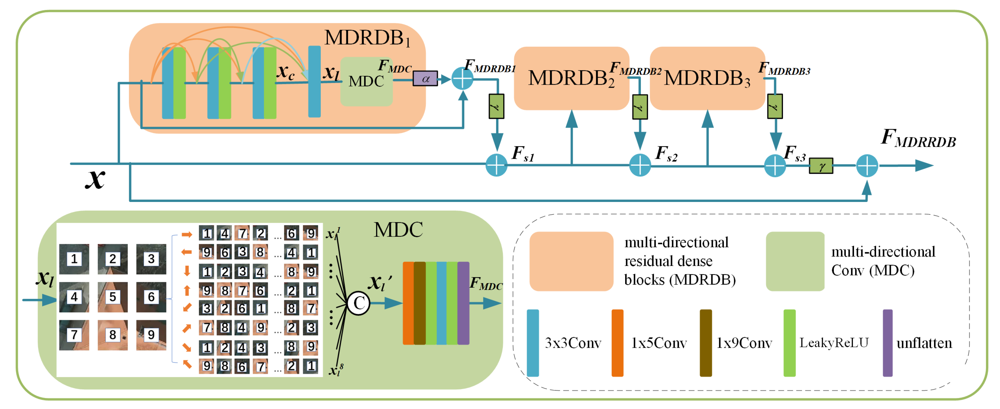
Viewing-angle variations significantly influence the dependency between target objects and their surrounding objects. Inspired by this mechanism, we propose the MDRRDB, which can explicitly capture the contextual relationships between objects from various directional perspectives. In the OFEM and DFEM, after shallow feature extraction via a 3 × 3 convolutional layer, we employ cascaded MDRRDB for deep feature extraction, enabling the derived deep features to capture more accurate cross-region contextual relationships. As shown in Figure 2, like RRDB, the MDRRDB is composed of three MDRDB stacked in a cascaded manner. We denote the input feature as x R H × W × C , which the operations of MDRRDB can be described as.
F M D R R D B = x + γ F s 3
F s i = F s i 1 + γ F M D R D B i , i = 2 , 3
F s 1 = x + γ F M D R D B 1
where γ is a hyperparameter, and here, we set it to 0.2. F M D R R D B R H × W × C represents the output feature of MDRRDB, and H M D R D B i represents the operations of i-th MDRDB.
Each MDRDB consists of multiple 3 × 3 convolutional layers and activation layers stacked together with residual connections and one multi-directional convolutional block (MDC), allowing the modeling of multi-directional spatial relationships in RSIs. In the stacked layers, the input of each layer is the result of the concatenation of the outputs from previous layers. Then all outputs from the stacked layers in MDRDB are concatenated and performed a convolution to generate the aggregated feature x l R H × W × C . This process can be described as follows:
x c = σ C o n v c x , x 1 , , x c 1 , c = 1 , 2 , 3
x l = C o n v 3 × 3 [ x , x 1 , , x C ]
where C o n v c and x c R H × W × C represent the c-th 3 × 3 convolutional layer and the output feature in the stacked layers. σ represents the LeakyReLU activation function.
In the MDC, for a given feature, x l , the feature is flattened along the height and width dimensions in eight directions (horizontal, vertical, principal diagonal, anti-diagonal, and their inverse directions); this operation is named MDflatten, and it results in a set of directional features, x l i i = 1 8 , where x l i R L × C , L = H × W . Next, the eight directional features are concatenated along the channel dimension to form a multi-directional joint feature, x l R L × C × 8 . Subsequently, two one-dimensional convolutions with different kernel sizes, followed by activation functions, are applied to extract local contextual information between different directions. Finally, a 3 × 3 convolution and an activation function are applied to the output, and the spatial dimensions are restored using an unflatten operation, yielding the output feature map, F M D C R H × W × C . Finally, F M D C is fused with the input feature, x, via residual connections. The above process can be mathematically expressed as follows:
x l = c o n c a t M D f l a t t e n x l
F M D C = u n f l a t t e n ( σ ( C o n v 3 × 3 ( σ ( C o n v 1 d x l ) ) ) )
F M D R D B = x + α F M D C x l
where α is a hyperparameter, and here we set it to 0.2. C o n v 1 d and σ represent the one-dimensional convolutions and LeakyReLU. M D f l a t t e n and u n f l a t t e n represent the operations of multi-directional flattening and its restoring.
By flattening features directionally and applying 1D convolutions, explicitly capture the associations between target objects and their environments from various directional perspectives. The multi-directional concatenation operation and 3 × 3 convolution further integrate multi-view contextual information.

3.3. Optical and DSM Fusion Module (ODF)

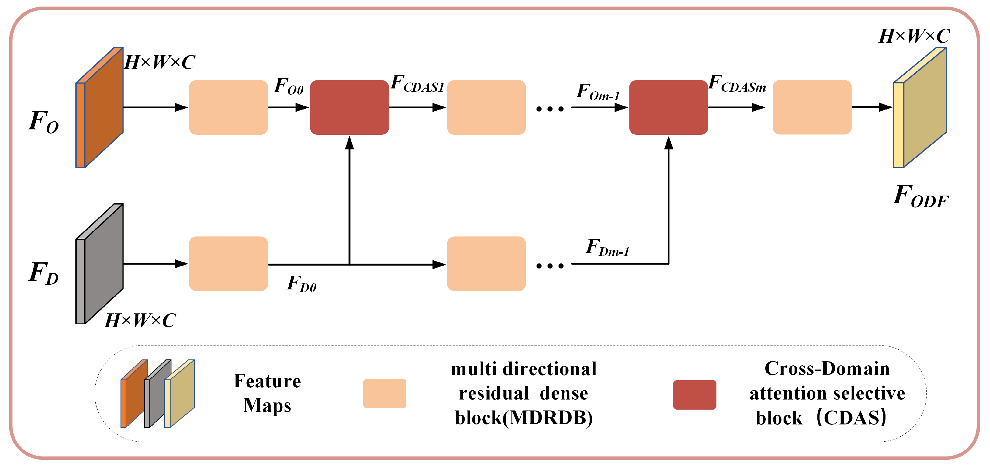
The ODF is designed to effectively integrate features F O and F D , which were independently extracted from OFEM and DFEM. To fully leverage these features in the subsequent reconstruction stage, the ODF progressively fuses F O and F D , ensuring that the details in F D can effectively replenish details that F O lacks. As shown in Figure 3, the ODF employs a progressive fusion strategy, which enhances both local detail preservation and global contextual coherence, composed of MDRDB and cross-domain attention selective blocks (CDAS). Specifically, the ODF consists of m CDAS and 2m + 1 MDRDB. Each CDAS receives features that have been processed via MDRDB from the two branches. The specific expression of the i-th CDAS is given as follows:
F C D A S i = H C D A S i F O i 1 , F D i 1 , i 1 , 2 , , m
where F C D A S i R H × W × C represents the output features of the i-th CDAS, and H C D A S i denotes the feature fusion operations of the i-th CDAS.
The fused feature F C D A S m R H × W × C is further processed via an MDRDB to obtain the final output features F O D F , expressed as follows:
F O D F = H M D R D B F C D A S m
Through this design, the ODF effectively integrates F O and F D , allowing the details in F D to enrich F O . This enables the F O D F with rich and comprehensive feature representations for the successive reconstruction task.
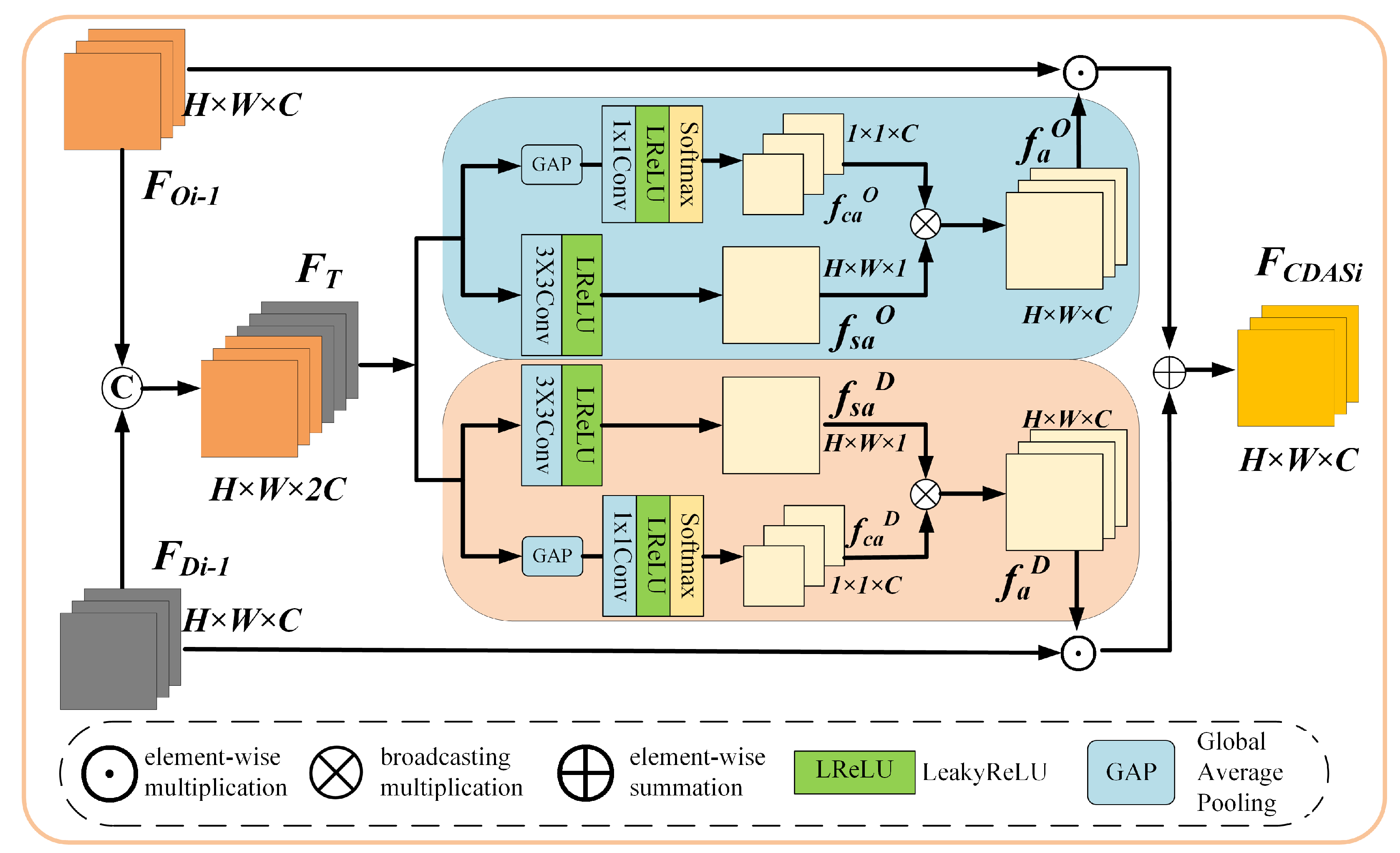
To better integrate features from different domains while selectively enhancing complementary similar features and suppressing dissimilar ones, we propose the CDAS. As shown in Figure 4, the CDAS first concatenates the two input features, F O i 1 R H × W × C and F D i 1 R H × W × C , along the channel dimension to form a new feature matrix, F T R H × W × 2 C . Then, F T is fed into two sets of operations; each set maintains an identical architecture composed of two parallel branches. In the first branch, global average pooling is applied to compress the spatial dimension of F T to 1 × 1. The resulting feature is then passed through a 1 × 1 convolution layer, followed by a LeakyReLU activation layer and a Softmax layer, yielding two channel attention vectors, f c a O , f c a D R 1 × 1 × C . In the second branch, F T is processed via a 3 × 3 convolution layer, followed by a LeakyReLU activation layer to generate two spatial attention matrices, f s a O , f s a D R H × W × 1 . Next, the attention features obtained from both branches are broadcast-multiplied to generate the cross-domain attention features, f a O , f a D R H × W × C :
f a O = f c a O × f s a O , f a D = f c a D × f s a D
where × represents broadcast multiplication.
Finally, f a O and f a D are multiplied elementwise with the input features F O i 1 F D i 1 , followed by a summation. This yields the fused feature representation F C D A S i R H × W × C , which contains both optical image and DSM information:
F C D A S i = s u m f a O F O i 1 , f a D F D i 1
where ⊙ denotes elementwise multiplication.

3.4. Fractal Mapping Super-Resolution Algorithm (FMA) and Fractal Loss Function

To leverage the abundant fractal-like texture patterns presented in RSIs, we propose FMA. Specifically, given an input, I L R R 3 × H × W , we utilize inherent self-similarity to generate a fractal-based SR image, I f r a R 3 × s H × s W , using a predefined mapping process, which can be denoted as follows:
I f r a = F FMA I L R ; s
where s represents the upscaling factor.
In FMA, we generate the pixel mapping relationship between I L R and I f r a through specific rules, thereby simulating the fractal process using the pixels of I L R to fill I f r a . Formally, the FMA can be described as a procedure that processes each position ( y , x ) of pixels in I L R , each position ( y f r a , x f r a ) , and its corresponding s × s block in the I f r a grid. For each position ( d y , d x ) within this block, the source coordinates ( y s r c , x s r c ) are computed as follows:
y s r c = y + d y [ s / 2 ]
x s r c = x + d x [ s / 2 ]
With the ( y s r c , x s r c ) , then, we can establish the mapping relationship between I f r a and  I L R :
I f r a [ y f r a , x f r a ] = I L R [ y s r c , x s r c ]
As the algorithm iterates, ( y f r a , x f r a ) is constantly updated. It is worth noting that the update for ( y f r a , x f r a ) is not linear but, rather, occurs through the stride mechanism. The specific update details are in Algorithm 1.
The generated I f r a is integrated into the model training process via a loss function, L f r a , to constrain the I S R towards solutions that exhibit statistical self-similarity across scales. Rather than relying solely on the network’s stochastic capability to hallucinate plausible textures, L f r a ensures that the generative process is guided by the inherent fractal regularity of RSIs. Therefore, the L f r a consists of the L1 loss between the model-generated image I S R and fractal-based SR image I f r a , which can be expressed as follows.
L f r a = | | I S R I f r a | | 1
where I S R represents the SR image from the DFMDN.
We use the L1 loss to minimize the spatial difference between SR and HR images.
L S R = | | I S R I H R | | 1
So, the total loss for the training can be denoted as follows:
L = L S R + λ L f r a
where λ is the regularization weight to balance the two loss functions, and here, we set it to 0.1.
Algorithm 1 Fractal Mapping Super-Resolution Algorithm
Input:
 optical image I LR R 3 × H × W , scaling factor s
Output:
 fractal-based SR image I fra R 3 × s H × s W
 
Initialize:
I fra zeros ( [ 3 , s H , s W ] )
δ y , δ x 0 , 0
stride _ state 0
Generate fractal coordinates:
for  ( y , x ) { 0 , , H 1 } × { 0 , , W 1 }   do
    for  ( d y , d x ) { 0 , , s 1 } × { 0 , , s 1 }  do
       y src y + d y s / 2
       x src x + d x s / 2
      if  ( d y + d x ) mod s = = 0  then
          δ y δ y + s / 2 stride _ state
          stride _ state ( stride _ state + 1 ) mod 2
      end if
      Update:
       I fra [ : , : , δ y , δ x ] I LR [ : , : , y src , x src ]
       δ x δ x + 1
      if  δ x s W  then
          δ x 0
          δ y δ y + 1
      end if
    end for
end for
return  I fra
Through the integration of L f r a as a constraint, the generation process is mathematically constrained to adhere to the principle of self-similarity. This ensures that the I S R natively exhibits multi-scale texture patterns that are statistically consistent with the fractal characteristics inherent to real-world RSIs, rather than relying solely on the network to learn these complex patterns from data alone.

4. Experimental Results and Analyses

4.1. Dataset

Our method is conducted experiments on three datasets, all containing DSM or DEM (in this paper, considering the similarity between DSM and DEM, we maintain consistent processing for DEM as with DSM), including two public datasets, Vaihingen and Potsdam [50,51], provided by the International Society for Photogrammetry and Remote Sensing (ISPRS), and one private dataset collected via satellites: County Dataset. All datasets were supplied as pre-registered data pairs in which each DSM(DEM) pixel is inherently aligned with its corresponding optical orthophoto pixel within a unified coordinate system. The following provides a detailed exposition.
Vaihingen: The Vaihingen dataset consists of 33 RSIs, with each orthophoto having three bands: near-infrared, red, and green. Additionally, it includes a normalized digital surface model (DSM) with a ground sampling distance (GSD) of 9 cm. We applied a sliding window method to crop the orthophotos and their corresponding DSM images into 256 × 256 patches with a stride of 256 pixels, resulting in a total of 2254 cropped image pairs. Of these, 90% were used as the training set, and the remaining 10% were used as the testing set.
Potsdam: The Potsdam dataset contains 38 very HR orthophotos, each with a size of 6000 × 6000 pixels. It provides multispectral data in four bands: infrared, red, green, and blue, along with a normalized DSM at a 5 cm GSD. The cropping method is the same as in Vaihingen, ultimately generating 20,102 cropped-image pairs.
County Dataset: This dataset is composed of remote sensing data from an administrative county collected by our team. Each orthorectified image contains three bands (RGB) with a spatial resolution of 0.5 m, along with a corresponding DEM at 0.5 m resolution. We cropped the RGB orthophotos and their corresponding DEM images into image pairs of 256 × 256 pixels. A total of 9336 image pairs were obtained, with 90% used for training and 10% for testing.

4.2. Evaluation Metrics and Implementation Details

In our experiments, we refer to near-infrared and infrared band images and visible light band images as optical images. We conducted experiments using scaling factors of ×2 and ×4. The optical LR images were degraded from optical HR images using bicubic down-sampling, and DSM remained at its original resolution without down-sampling. The SR results were evaluated with the peak signal-to-noise ratio (PSNR) and the structural similarity index measure (SSIM) [52].
For our DFMDN, we set the number of MDRRDB to 3, RRDB to 15, and CDAS to 2. The model was trained and optimized using the Adam optimizer [53], with hyperparameters β 1 = 0.9, β 2 = 0.999, and ϵ = 10 8 . We randomly selected 16 LR patches as the input to the model. Considering the significant differences in resolution among the datasets, we trained the model separately on each training set. Specifically, the Potsdam and the County Datasets were trained for 100,000 iterations, while the Vaihingen dataset underwent 50,000 iterations. The initial learning rate was set to 2 × 10 4 and halved after 50,000 iterations. We implemented our method using PyTorch 1.8.2, and all experiments were conducted on an NVIDIA GeForce GTX 3090 GPU.

4.3. Comparison with the State-of-the-Arts

In this section, we compare the proposed model with several state-of-the-art (SOTA) algorithms, including EDSR [26], RRDBNet [28], RCAN [29], CTNet [54], HSENet [23], MHAN [17], and TTST [55]. Among these, EDSR [26], RRDBNet [28], and RCAN [29] are general image SR methods. CTNet [54], HSENet [23], MHAN [17], and TTST [55] are the most advanced SR methods for RSIs. To ensure a fair comparison, we trained and tested all algorithms on the same datasets, using the official code provided via the respective authors.

4.3.1. Quantitative Comparison

Table 1 presents the results of the quantitative comparison. In each row, the best and second best results are bolded and underlined. From Table 1, it can be observed that, on both test datasets, DFMDN achieves nearly all the best performances in terms of PSNR and SSIM. Due to the high spatial resolution of the two test datasets, the SISR methods EDSR, RCAN, and RRDBNet have demonstrated strong performance. Especially in the Vaihingen test set, RCAN outperforms RSISR methods CTNet, HSENet, and MHAN, when the scaling factor is set to 2, but our method is better than RCAN. It is worth noting that our method improves PSNR by 0.66 dB compared to RRDBNet. This clearly highlights the effectiveness of incorporating DSM priors and MDRRDB. When the scaling factor is set to 2 in the Potsdam test dataset, RCAN, MHAN, and TTST deliver nearly identical results, however, our method achieves an additional improvement of 0.25 dB in PSNR. Meanwhile, TTST, as the most advanced Transformer-based RSISR approach, exhibits consistently stable performance compared to the other RSISR methods CTNet, HSENet, and MHAN across different scales on both test datasets. However, DFMDN’s performance surpasses TTST in all test datasets, especially in the Vaihingen test set, when the scaling factor is set to 4, our method improves PSNR by 0.14dB, which underscores TTST’s weaker performance on small sample datasets. With the spatial resolution further increased in the Potsdam dataset, the SISR method achieves even better results. Specifically, when the scaling factor is set to 4, RCAN’s performance surpasses TTST. Nevertheless, our approach still offers an improvement over both RCAN and TTST; this may be attributed to our method’s ability to leverage richer contextual relationships for image reconstruction.

4.3.2. Qualitative Comparison

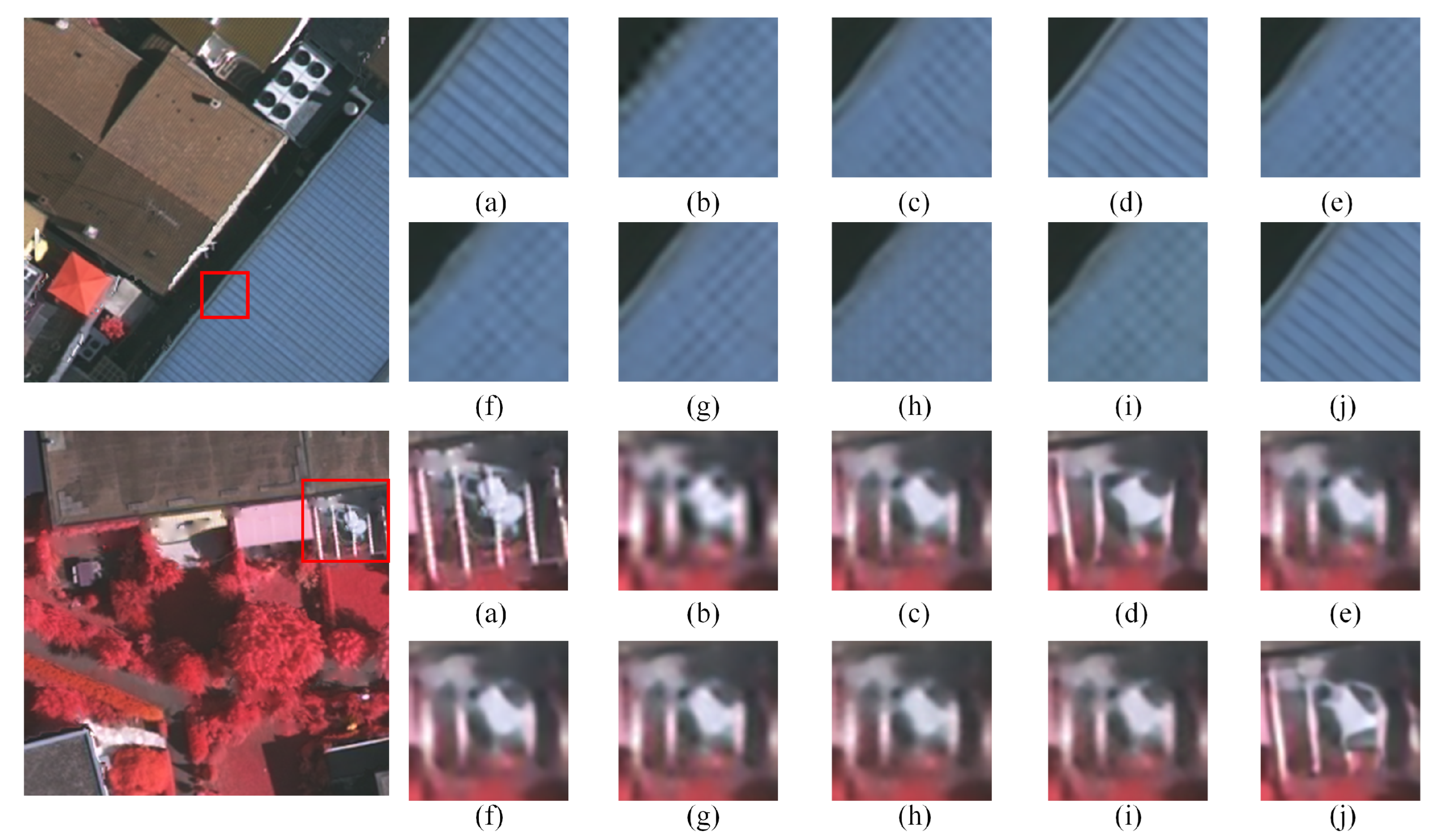
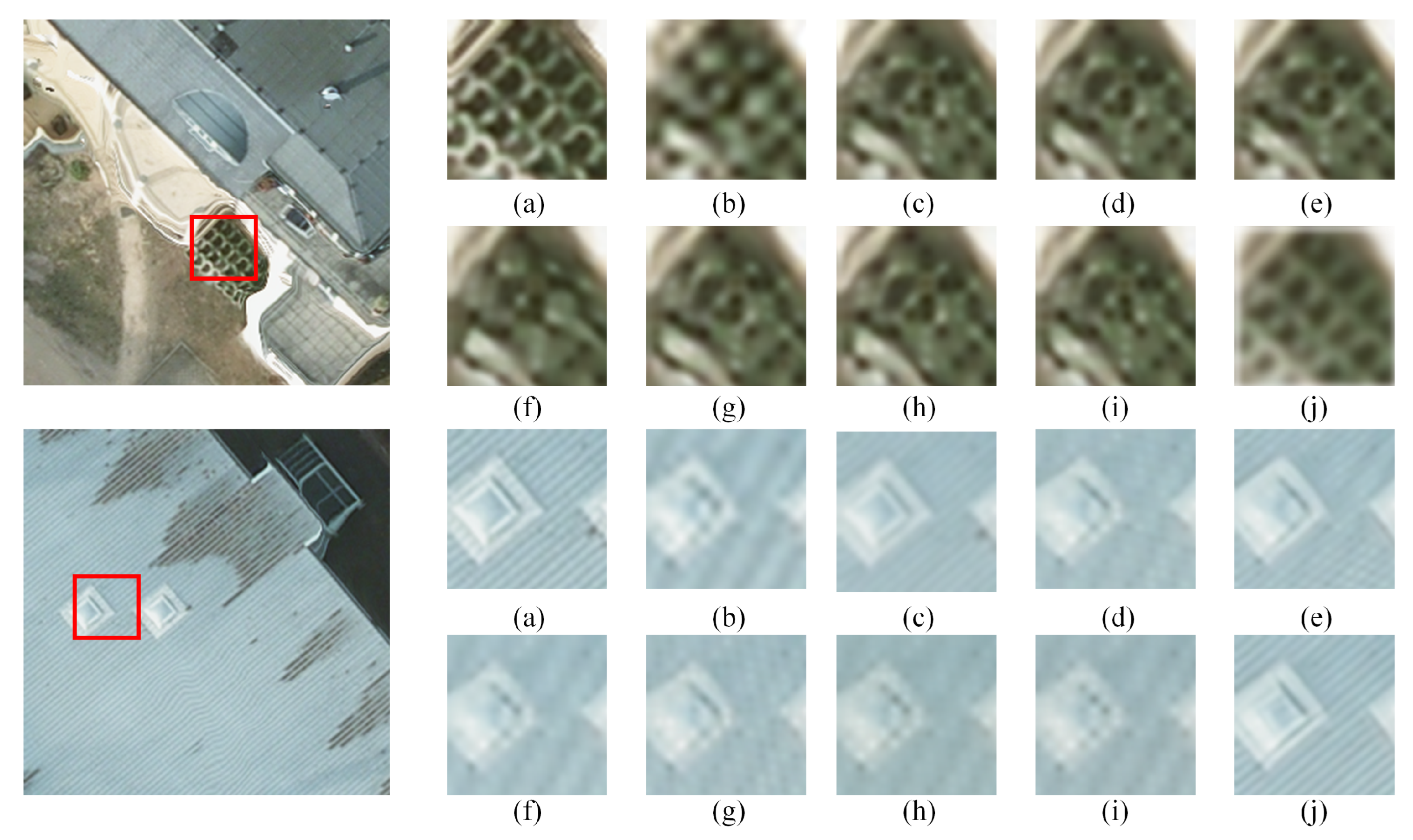
The qualitative comparison results are presented in Figure 5 and Figure 6, from which it can be observed that our method produces results that appear more natural and realistic compared to other approaches. For instance, for the reconstruction of the blue roof of ”patch of area4” in Figure 5, while the other methods exhibited incorrect textures, only our method and RRDBNet successfully reconstructed the correct texture. Furthermore, compared to RRDBNet, our method restores textures with greater clarity. In the railing region of the ”patch of area35” in Figure 5, owing to MDC, which enables a better modeling of texture directions in texture-dense regions, only our method successfully reconstructs the railing, while the other methods incorrectly merge the railing with the obstructing object. Because of the prior information provided via DSM, our model demonstrates strong recovery capabilities at edges. In ”patch of 02-14” of Figure 6, our method successfully reconstructed the wire mesh with high fidelity, while other methods failed to recover the grid structure. In ”patch of 04-13” of Figure 6, EDSR, CTNet, HSENet, and TTST generate artifacts or incorrect texture patterns. In contrast, our method successfully restores the correct texture pattern with high fidelity.

4.4. Complexity Analysis

To comprehensively evaluate the practical efficiency of our proposed DFMDN model, we compare its computational complexity with the aforementioned methods. The comparison is conducted in terms of two critical metrics: the number of parameters (Params) and floating-point operations (FLOPs) and the actual inference time. Please note that the size of our input images should be kept consistent with that used during training. The result is summarized in Table 2.
Our DFMDN model contains 13.89 million parameters and requires 62.03 GFLOPs, achieving an inference time of 0.39 s to process a single image. Compared to the lightweight CTNet (0.35 M Params, 1.04 G FLOPs), HSENet (5.29 M Params, 16.70 G FLOPs), DFMDN is more complex, which is a deliberate design choice to achieve higher reconstruction fidelity. However, when contrasted with other high-performance models such as RRDBNet (16.70 M Params, 73.43 G FLOPs, 0.38 s), MHAN (11.20M Params, 46.31 G FLOPs, 0.36 s), TTST (18.30 M Params, 76.84 G FLOPs, 0.42 s), and RCAN (12.61 M Params, 53.16 G FLOPs, 0.54 s), DFMDN achieves good results with almost the same complexity. In particular, compared to TTST and RCAN, DFMDN achieves a faster inference speed and better performance, which also proves the effectiveness of our model approach, demonstrating a favorable trade-off between model capacity and computational costs.

4.5. Statistical Significance Analysis

To rigorously validate the performance superiority of our proposed DFMDN model over the TTST, we conducted a comprehensive statistical significance analysis using the Wilcoxon signed-rank test based on 10 independent experimental runs of different random seeds. The null hypothesis ( H 0 ) states that there is no significant performance difference between DFMDN and the TTST, while the alternative hypothesis ( H 1 ) states that a significant difference exists. A p-value less than 0.05 indicates statistical significance at the 95% confidence level. The quantitative results are summarized in Table 3.
The statistical analysis reveals that our DFMDN model achieves significantly superior performance compared to TTST across both key metrics. Specifically, DFMDN attains a mean PSNR of 40.959 ± 0.028 dB, substantially outperforming TTST’s 40.755 ± 0.032 dB. More importantly, a Wilcoxon signed-rank test confirms that this improvement is statistically significant with a p-value of 0.0020 ( p < 0.05 ).
Similarly, in terms of structural similarity, DFMDN achieves a mean SSIM of 0.9696 ± 0.0003 , compared to TTST’s 0.9688 ± 0.0004 . The statistical significance test yields a p-value of 0.0020 ( p < 0.05 ), providing strong evidence that the SSIM improvement is not due to random chance.

4.6. Ablation Experiments

In this section, we conduct ablation studies to investigate the importance of the proposed components in our method, including the hyperparameter λ , MDRRDB, DFEM, ODF, FMA, and the number of directions in MDRRDB and the number of CDAS in ODF.

4.6.1. Study of λ

The hyperparameter λ controls the weight of the fractal loss in the overall loss composition. Based on our experiments, setting 0.1 < λ < 0.5 yields optimal performance. Within this range, we evaluated values of 0.1, 0.2, 0.3, 0.4, and 0.5. The results, detailed in Table 4, demonstrate that the model achieves the best performance when λ = 0.1 . Therefore, we set λ = 0.1 in the final model configuration.

4.6.2. Effectiveness of the DFEM, ODF, and MDRRDB

In this work, we employ DFEM as part of DFMDN to provide DSM-based prior information for image reconstruction. To validate the effectiveness of DFEM, we remove it and present the performance comparison of different model configurations in Table 5. The experimental results demonstrate that the removal of DFEM leads to a 0.17 dB decrease in PSNR. Thus, the above experiments confirm the efficacy of DFEM. The results indicate that high-quality image priors are beneficial for image reconstruction. The role of ODF is to fuse features from OFEM and DFEM, enabling DFEM features to fully assist in edge detail generation. To verify the effectiveness of ODF, we replace it with a summation operation, with the results also shown in Table 5. The experimental results reveal that removing ODF degrades quantitative performance compared to DFMDN, with a 0.1 dB reduction in PSNR. MDRRDB is designed to capture the contextual relationships between objects in different directions. To evaluate the effectiveness of MDRRDB, we replace it with RRDB. The experimental results indicate that removing the MDRRDB results in a 0.08 dB decrease in PSNR.

4.6.3. Effectiveness of the FMA

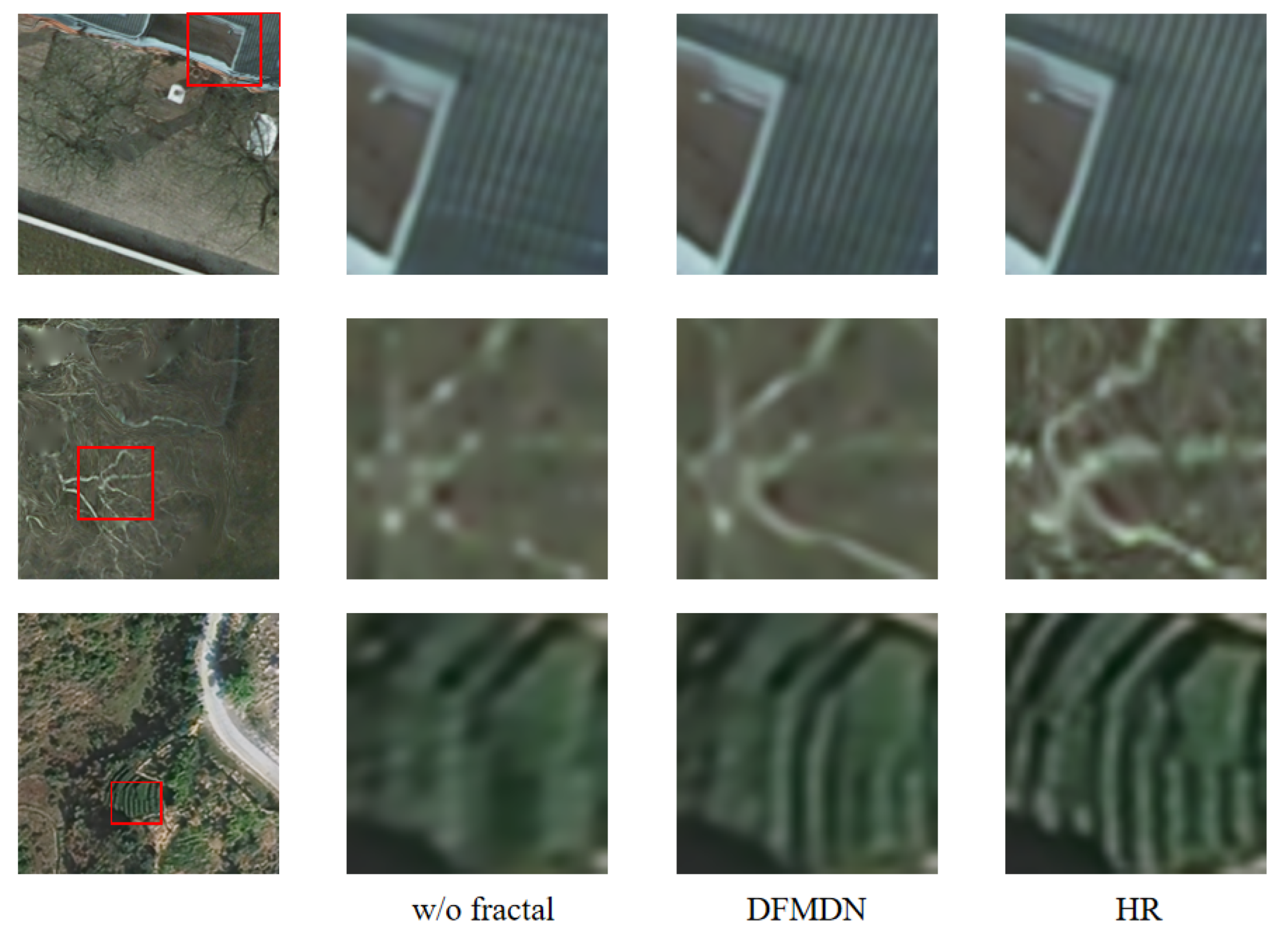
In this work, we employ FMA and a related loss to enhance natural textures in reconstructed images. To validate the effectiveness of FMA, we train the model on the same dataset without using this component. The results in Figure 7 demonstrate the impact of FMA: For the first row, incorporating the fractal term eliminates horizontal artifacts. In the second row, it enriches texture details. For the third row, it produces edge details that better align with the ground truth.

4.6.4. Study of the ODF

In the ODF, we design the CDAS block for feature fusion. To validate the effectiveness of CDAS, we conduct ablation studies by replacing it with alternative fusion strategies: channel attention, element-wise summation, and channel concatenation. The experimental results in Table 6 demonstrate that all alternative approaches underperform the proposed DFMDN framework, with the PSNR metric decreasing by over 0.1 dB when CDAS is removed.

4.6.5. Study of the Number of Directions in MDRRDB

To further validate the effectiveness of our proposed MDRRDB, we conducted an ablation study on the number of flattening directions in MDRRDB. In Table 7, ”8” denotes the number of directions illustrated in Figure 2, while ”4” represents only the horizontal and vertical directions, and their reverse directions, and ”2” indicates only the horizontal directions and its reverse direction. ”1” means no multi-directional flattening, like that in other methods, is applied. As shown in Table 7, the performance metrics gradually improve as the number of directions increases. This is because extracting relationships from different directions further enriches the captured features while ensuring the correctness of the extracted relationships.

4.6.6. Study of the Number of CDAS in ODF

To validate how many CDAS are sufficient to effectively integrate features from different domains, we conducted experiments. As shown in Table 8, ”1”, ”2”, and other numbers represent the number of CDAS in ODF. The performance metrics gradually improve with an increasing number of CDAS, with the most significant improvement observed when increasing from 1 to 2 CDAS. This is attributed to the progressive feature fusion strategy, which thoroughly combines shallow and deep-level features to extract richer representations. However, further increasing the number of CDAS has little effect on performance improvements. To strike a balance between efficiency and performance, the final version adopts 2 CDAS in ODF.

4.7. Experiments on a County Dataset

To further validate the effectiveness of DFMDN across varying resolutions and complex scenarios, we conducted additional experiments on the County dataset. Due to the proprietary nature of this dataset, we present only partial reconstruction results and partial ablation studies. As illustrated in Figure 8, DFMDN achieves satisfactory reconstruction performance, particularly in preserving edge details and texture. The ablation results in Table 9 demonstrate consistent performance trends with those observed on the Potsdam dataset. These experiments confirm that our proposed components—DFEM, ODF, and MDRRDB—maintain their effectiveness across different resolution scales, diverse degradation scenarios and varied environmental conditions.

5. Conclusions

In this paper, we have proposed DFMDN, a novel deep learning framework for RSISR. The proposed DFMDN consists of two key parts: OFEM and DFEM, with feature fusion performed via the ODF. Additionally, we introduce a fractal mapping algorithm incorporated into the training process via a dedicated loss function. Extensive experiments conducted on two public datasets and one real-world proprietary dataset demonstrate that DFMDN achieves competitive performance compared to SOTA methods. Quantitative and qualitative results validate the effectiveness of each proposed component, particularly in preserving fine edge details and natural textures across varying resolutions and complex scenes. For future work, we will focus on integrating more domain-specific prior knowledge (such as the DSM and fractal features explored in this study) into deep learning architectures. We believe this direction holds significant promise for advancing remote sensing image processing technologies, particularly in scenarios requiring high-fidelity reconstruction under challenging degradation conditions.

Author Contributions

Conceptualization, S.L. and B.Z.; methodology, S.L. and B.Z.; software, J.H. and B.Z.; validation, J.H. and B.Z.; formal analysis, S.L. and J.H.; investigation, J.H. and B.Z.; resources, S.L.; data curation, J.H.; writing—original draft preparation, S.L. and J.H.; writing—review and editing, S.L. and J.H.; visualization, J.H.; supervision, S.L. and B.Z.; project administration, S.L. and B.Z.; funding acquisition, S.L. All authors have read and agreed to the published version of the manuscript.

Funding

This research was funded by the National Natural Science Foundation of China under Grant 61971306.

Institutional Review Board Statement

Not applicable.

Informed Consent Statement

Not applicable.

Data Availability Statement

These data were derived from the following resources that are available in the public domain: ISPRS Potsdam 2D Semantic Labeling Dataset, https://www.kaggle.com/datasets/aletbm/urban-segmentation-isprs, accessed on 17 October 2025, and the data of private dataset, County Dataset, will be made available by the authors upon request.

Conflicts of Interest

The authors declare no conflicts of interest.

References

  1. Pruitt, E.L. The office of naval research and geography. Ann. Assoc. Am. Geogr. 1979, 69, 103–108. [Google Scholar] [CrossRef]
  2. Lillesand, T.; Kiefer, R.W.; Chipman, J. Remote Sensing and Image Interpretation; John Wiley & Sons: Hoboken, NJ, USA, 2015. [Google Scholar]
  3. Tucker, C.J.; Townshend, J.R.; Goff, T.E. African land-cover classification using satellite data. Science 1985, 227, 369–375. [Google Scholar] [CrossRef]
  4. Tralli, D.M.; Blom, R.G.; Zlotnicki, V.; Donnellan, A.; Evans, D.L. Satellite remote sensing of earthquake, volcano, flood, landslide and coastal inundation hazards. ISPRS J. Photogramm. Remote Sens. 2005, 59, 185–198. [Google Scholar] [CrossRef]
  5. Williams, D.L.; Goward, S.; Arvidson, T. Landsat. Photogramm. Eng. Remote Sens. 2006, 72, 1171–1178. [Google Scholar] [CrossRef]
  6. Schowengerdt, R.A. Remote Sensing: Models and Methods for Image Processing; Elsevier: Amsterdam, The Netherlands, 2006. [Google Scholar]
  7. Nakazawa, S.; Iwasaki, A. Super-resolution imaging using remote sensing platform. In Proceedings of the 2014 IEEE Geoscience and Remote Sensing Symposium, Quebec City, QC, Canada, 13–18 July 2014; IEEE: Piscataway, NJ, USA, 2014; pp. 1987–1990. [Google Scholar]
  8. Vishnukumar, S.; Wilscy, M. Super-resolution for remote sensing images using content adaptive detail enhanced self examples. In Proceedings of the 2016 International Conference on Circuit, Power and Computing Technologies (ICCPCT), Nagercoil, India, 18–19 March 2016; IEEE: Piscataway, NJ, USA, 2016; pp. 1–5. [Google Scholar]
  9. Tu, T.M.; Su, S.C.; Shyu, H.C.; Huang, P.S. A new look at IHS-like image fusion methods. Inf. Fusion 2001, 2, 177–186. [Google Scholar] [CrossRef]
  10. Vivone, G.; Alparone, L.; Chanussot, J.; Dalla Mura, M.; Garzelli, A.; Licciardi, G.A.; Restaino, R.; Wald, L. A critical comparison among pansharpening algorithms. IEEE Trans. Geosci. Remote Sens. 2014, 53, 2565–2586. [Google Scholar] [CrossRef]
  11. González-Audícana, M.; Saleta, J.L.; Catalán, R.G.; García, R. Fusion of multispectral and panchromatic images using improved IHS and PCA mergers based on wavelet decomposition. IEEE Trans. Geosci. Remote Sens. 2004, 42, 1291–1299. [Google Scholar] [CrossRef]
  12. Masi, G.; Cozzolino, D.; Verdoliva, L.; Scarpa, G. Pansharpening by convolutional neural networks. Remote Sens. 2016, 8, 594. [Google Scholar] [CrossRef]
  13. Liebel, L.; Körner, M. Single-image super resolution for multispectral remote sensing data using convolutional neural networks. Int. Arch. Photogramm. Remote Sens. Spat. Inf. Sci. 2016, 41, 883–890. [Google Scholar] [CrossRef]
  14. Haut, J.M.; Fernandez-Beltran, R.; Paoletti, M.E.; Plaza, J.; Plaza, A.; Pla, F. A new deep generative network for unsupervised remote sensing single-image super-resolution. IEEE Trans. Geosci. Remote Sens. 2018, 56, 6792–6810. [Google Scholar] [CrossRef]
  15. Haut, J.M.; Paoletti, M.E.; Fernández-Beltran, R.; Plaza, J.; Plaza, A.; Li, J. Remote sensing single-image superresolution based on a deep compendium model. IEEE Geosci. Remote Sens. Lett. 2019, 16, 1432–1436. [Google Scholar] [CrossRef]
  16. Wang, Y.; Shao, Z.; Lu, T.; Wu, C.; Wang, J. Remote sensing image super-resolution via multiscale enhancement network. IEEE Geosci. Remote Sens. Lett. 2023, 20, 5000905. [Google Scholar] [CrossRef]
  17. Zhang, D.; Shao, J.; Li, X.; Shen, H.T. Remote sensing image super-resolution via mixed high-order attention network. IEEE Trans. Geosci. Remote Sens. 2021, 59, 5183–5196. [Google Scholar] [CrossRef]
  18. He, D.; Zhong, Y. Deep hierarchical pyramid network with high-frequency-aware differential architecture for super-resolution mapping. IEEE Trans. Geosci. Remote Sens. 2023, 61. [Google Scholar] [CrossRef]
  19. Huan, H.; Li, P.; Zou, N.; Wang, C.; Xu, D. End-to-End Super-Resolution for Remote-Sensing Images Using an Improved Multi-Scale Residual Network. Remote Sens. 2021, 13, 666. [Google Scholar] [CrossRef]
  20. Jiang, K.; Wang, Z.; Yi, P.; Wang, G.; Lu, T.; Jiang, J. Edge-enhanced GAN for remote sensing image super resolution. IEEE Trans. Geosci. Remote Sens. 2019, 57, 5799–5812. [Google Scholar] [CrossRef]
  21. Li, H.; Deng, W.; Zhu, Q.; Guan, Q.; Luo, J. Local-Global Context-Aware Generative Dual-Region Adversarial Networks for Remote Sensing Scene Image Super-Resolution. IEEE Trans. Geosci. Remote Sens. 2024, 62, 5402114. [Google Scholar] [CrossRef]
  22. Zhao, S.; Chen, H.; Zhang, X.; Xiao, P.; Bai, L.; Ouyang, W. RS-Mamba for Large Remote Sensing Image Dense Prediction. IEEE Trans. Geosci. Remote Sens. 2024, 62, 5633314. [Google Scholar] [CrossRef]
  23. Lei, S.; Shi, Z. Hybrid-scale self-similarity exploitation for remote sensing image super-resolution. IEEE Trans. Geosci. Remote Sens. 2022, 60, 5401410. [Google Scholar] [CrossRef]
  24. Dong, C.; Loy, C.C.; He, K.; Tang, X. Image super-resolution using deep convolutional networks. IEEE Trans. Pattern Anal. Mach. Intell. 2016, 38, 295–307. [Google Scholar] [CrossRef]
  25. Kim, J.; Lee, J.K.; Lee, K.M. Accurate image super-resolution using very deep convolutional networks. In Proceedings of the IEEE Conference on Computer Vision and Pattern Recognition, Las Vegas, NV, USA, 26 June–1 July 2016; pp. 1646–1654. [Google Scholar]
  26. Lim, B.; Son, S.; Kim, H.; Nah, S.; Lee, K.M. Enhanced deep residual networks for single image super-resolution. In Proceedings of the IEEE Conference on Computer Vision and Pattern Recognition, Workshops, Honolulu, HI, USA, 21–26 July 2017; pp. 136–144. [Google Scholar]
  27. Ledig, C.; Theis, L.; Huszár, F.; Caballero, J.; Cunningham, A.; Acosta, A.; Aitken, A.; Tejani, A.; Totz, J.; Wang, Z.; et al. Photo-realistic single image super-resolution using a generative adversarial network. In Proceedings of the IEEE Conference on Computer Vision and Pattern Recognition, Honolulu, HI, USA, 21–26 July 2017; pp. 4681–4690. [Google Scholar]
  28. Wang, X.; Yu, K.; Wu, S.; Gu, J.; Liu, Y.; Dong, C.; Qiao, Y.; Change Loy, C. ESRGAN: Enhanced super-resolution generative adversarial networks. In Proceedings of the European Conference on Computer Vision Workshops, Munich, Germany, 20–22 September 2019; pp. 63–79. [Google Scholar]
  29. Zhang, Y.; Li, K.; Li, K.; Wang, L.; Zhong, B.; Fu, Y. Image super-resolution using very deep residual channel attention networks. In Proceedings of the European Conference on Computer Vision, Munich, Germany, 8–14 September 2018; pp. 286–301. [Google Scholar]
  30. Dai, T.; Cai, J.; Zhang, Y.; Xia, S.T.; Zhang, L. Second-order attention network for single image super-resolution. In Proceedings of the IEEE Conference on Computer Vision and Pattern Recognition, Long Beach, CA, USA, 16–20 June 2019; pp. 11065–11074. [Google Scholar]
  31. Liang, J.; Cao, J.; Sun, G.; Zhang, K.; Van Gool, L.; Timofte, R. SwinIR: Image restoration using Swin transformer. In Proceedings of the IEEE/CVF International Conference on Computer Vision Workshops, Virtual, 11–17 October 2021; pp. 1833–1844. [Google Scholar]
  32. Liu, C.; Yang, H.; Fu, J.; Qian, X. Learning trajectory-aware transformer for video super-resolution. In Proceedings of the IEEE/CVF Conference on Computer Vision and Pattern Recognition, New Orleans, LA, USA, 18–24 June 2022; pp. 5687–5696. [Google Scholar]
  33. Chen, X.; Wang, X.; Zhou, J.; Dong, C. Activating more pixels in image super-resolution transformer. In Proceedings of the IEEE Conference on Computer Vision and Pattern Recognition, Vancouver, BC, Canada, 18–22 June 2023; pp. 22367–22377. [Google Scholar]
  34. Yekeben, Y.; Cheng, S.; Du, A. CGFTNet: Content-Guided Frequency Domain Transform Network for Face Super-Resolution. Information 2024, 15, 765. [Google Scholar] [CrossRef]
  35. Yao, X.; Pan, Y.; Wang, J. An omnidirectional image super-resolution method based on enhanced SwinIR. Information 2024, 15, 248. [Google Scholar] [CrossRef]
  36. Lei, S.; Shi, Z.; Zou, Z. Super-resolution for RSIs via local–global combined network. IEEE Geosci. Remote Sens. Lett. 2017, 14, 1243–1247. [Google Scholar] [CrossRef]
  37. Lu, T.; Wang, J.; Zhang, Y.; Wang, Z.; Jiang, J. Satellite image super-resolution via multi-scale residual deep neural network. Remote Sens. 2019, 11, 1588. [Google Scholar] [CrossRef]
  38. Ma, C.; Rao, Y.; Cheng, Y.; Chen, C.; Lu, J.; Zhou, J. Structure-preserving super resolution with gradient guidance. In Proceedings of the IEEE/CVF Conference on Computer Vision and Pattern Recognition, Seattle, WA, USA, 14–19 June 2020; pp. 7769–7778. [Google Scholar]
  39. Zhao, K.; Lu, T.; Wang, J.; Zhang, Y.; Jiang, J.; Xiong, Z. Hyper-Laplacian Prior for Remote Sensing Image Super-Resolution. IEEE Trans. Geosci. Remote Sens. 2024, 62, 5634514. [Google Scholar] [CrossRef]
  40. Jia, S.; Wang, Z.; Li, Q.; Jia, X.; Xu, M. Multiattention Generative Adversarial Network for Remote Sensing Image Super-Resolution. IEEE Trans. Geosci. Remote Sens. 2022, 60, 5624715. [Google Scholar] [CrossRef]
  41. Dong, R.; Zhang, L.; Fu, H. RRSGAN: Reference-Based Super-Resolution for Remote Sensing Image. IEEE Trans. Geosci. Remote Sens. 2022, 60, 5601117. [Google Scholar] [CrossRef]
  42. Tu, Z.; Yang, X.; He, X.; Yan, J.; Xu, T. RGTGAN: Reference-Based Gradient-Assisted Texture-Enhancement GAN for Remote Sensing Super-Resolution. IEEE Trans. Geosci. Remote Sens. 2024, 62, 5607221. [Google Scholar] [CrossRef]
  43. Meng, F.; Wu, S.; Li, Y.; Zhang, Z.; Feng, T.; Liu, R.; Du, Z. Single remote sensing image super-resolution via a generative adversarial network with stratified dense sampling and chain training. IEEE Trans. Geosci. Remote Sens. 2023, 62, 5400822. [Google Scholar] [CrossRef]
  44. Cannon, J.W.; Floyd, W.J.; Parry, W.R. Crystal growth, biological cell growth, and geometry. In Pattern Formation in Biology: Vision, and Dynamics; World Scientific: Singapore, 2000; pp. 65–82. [Google Scholar]
  45. Lowe, D.G. Object recognition from local scale-invariant features. In Proceedings of the Seventh IEEE International Conference on Computer Vision, Kerkyra, Greece, 20–27 September 1999; IEEE: Piscataway, NJ, USA, 1999; Volume 2, pp. 1150–1157. [Google Scholar]
  46. Ghazel, M.; Freeman, G.H.; Vrscay, E.R. Fractal image denoising. IEEE Trans. Image Process. 2003, 12, 1560–1578. [Google Scholar] [CrossRef]
  47. Zhang, Y.; Fan, Q.; Bao, F.; Liu, Y.; Zhang, C. Single-Image Super-Resolution Based on Rational Fractal Interpolation. IEEE Trans. Image Process. 2018, 27, 3782–3797. [Google Scholar] [CrossRef]
  48. Hua, Z.; Zhang, H.; Li, J. Image Super Resolution Using Fractal Coding and Residual Network. Complexity 2019, 2019. [Google Scholar] [CrossRef]
  49. Song, X.; Liu, W.; Liang, L.; Shi, W.; Xie, G.; Lu, X.; Hei, X. Image super-resolution with multi-scale fractal residual attention network. Comput. Graph. 2023, 113, 21–31. [Google Scholar] [CrossRef]
  50. Rottensteiner, F.; Sohn, G.; Jung, J.; Gerke, M.; Baillard, C.; Benitez, S.; Breitkopf, U. The ISPRS benchmark on urban object classification and 3D building reconstruction. ISPRS Ann. Photogramm. Remote Sens. Spat. Inf. Sci. 2012, I-3, 293–298. [Google Scholar] [CrossRef]
  51. Wang, L.; Li, R.; Zhang, C.; Fang, S.; Duan, C.; Meng, X.; Atkinson, P.M. UNetFormer: A UNet-like transformer for efficient semantic segmentation of remote sensing urban scene imagery. ISPRS J. Photogramm. Remote Sens. 2022, 190, 196–214. [Google Scholar] [CrossRef]
  52. Zhou, W.; Bovik, A.C.; Sheikh, H.R.; Simoncelli, E.P. Image quality assessment: From error visibility to structural similarity. IEEE Trans. Image Process. 2004, 13, 600–612. [Google Scholar] [CrossRef] [PubMed]
  53. Kingma, D.P.; Ba, J. Adam: A method for stochastic optimization. arXiv 2014, arXiv:1412.6980. [Google Scholar]
  54. Wang, S.; Zhou, T.; Lu, Y.; Di, H. Contextual transformation network for lightweight remote-sensing image super-resolution. IEEE Trans. Geosci. Remote Sens. 2022, 60, 1–13. [Google Scholar] [CrossRef]
  55. Xiao, Y.; Yuan, Q.; Jiang, K.; He, J.; Lin, C.W.; Zhang, L. TTST: A top-k token selective transformer for remote sensing image super-resolution. IEEE Trans. Image Process. 2024, 33, 738–752. [Google Scholar] [CrossRef]
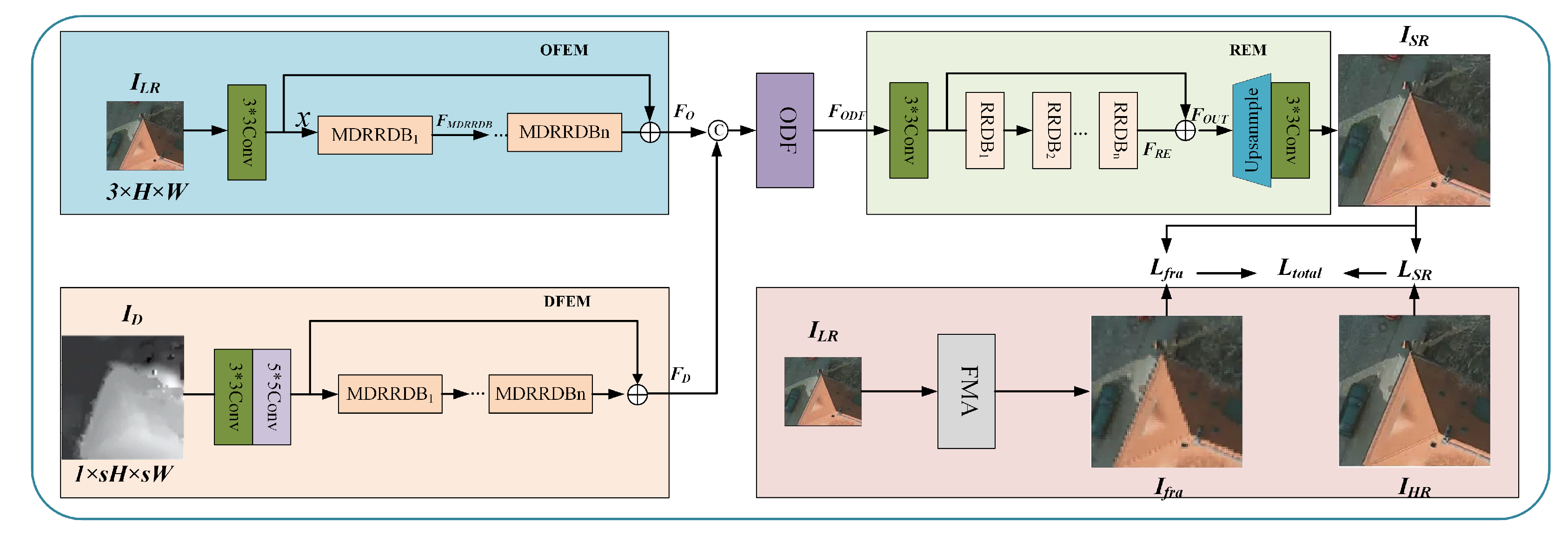
Figure 1. Overall structure of proposed digital elevation data and fractal-guided multi-directional super resolution network (DFMDN).
Information 16 01020 g001
Figure 2. Details of our proposed multi-directional residual-in-residual dense blocks (MDRRDB) (top) and the architecture of multi-directional convolutional block (MDC) (bottom left).
Information 16 01020 g002
Figure 3. Proposed optical and DSM fusion module (ODF).
Information 16 01020 g003
Figure 4. The details of our proposed cross-domain attention selective blocks (CDAS).
Information 16 01020 g004
Figure 5. Visual comparisons with different methods on ”patch of area4” (top) and ”patch of area35” (bottom) samples of Vaihingen, whose scale is ×4. (a) HR. (b) Bicubic. (c) EDSR. (d) RRDBNet. (e) RCAN. (f) CTNet. (g) HSENet. (h) MHAN. (i) TTST. (j) Ours.
Information 16 01020 g005
Figure 6. Visual comparisons with different methods on ”patch of 02-14” (top) and ”patch of 04-13”(bottom) samples of Potsdam, whose scale is ×4. (a) HR. (b) Bicubic. (c) EDSR. (d) RRDBNet. (e) RCAN. (f) CTNet. (g) HSENet. (h) MHAN. (i) TTST. (j) Ours.
Information 16 01020 g006
Figure 7. The ablation experiment for the FMA on different test datasets for 4× SR. w/o indicates that the FMA was not added during training.
Information 16 01020 g007
Figure 8. Visual comparisons on the County datasets for 4× SR.
Information 16 01020 g008
Table 1. Quantitative results for Scale 2× SR and 4× SR on the Vaihingen and Potsdam Test Set.
MethodScaleVaihingenPotsdam
PSNR SSIM PSNR SSIM
Bicubic × 2 34.91000.943337.95000.9573
EDSR37.45750.965540.66850.9679
RCAN37.84210.967940.70800.9685
RRDBNet37.19780.963640.33930.9663
CTNet36.98650.962640.35670.9668
HSENet37.48130.965840.68470.9681
MHAN37.58790.966340.74050.9683
TTST37.81650.967840.75550.9688
DFMDN (ours)37.86220.968240.95910.9696
Bicubic × 4 27.93000.808630.06000.8051
EDSR29.83810.854032.73180.8631
RCAN29.63310.856433.03100.8646
RRDBNet29.78390.853833.01460.8641
CTNet29.40210.842532.36860.8533
HSENet29.71860.853432.80000.8604
MHAN29.61250.850332.98950.8636
TTST29.86670.856432.98340.8635
DFMDN (ours)30.00230.857833.07960.8644
Table 2. Analysis of model complexity.
ModelParams (M)FLOPs (G)Time (s)
EDSR1.528.120.32
RCAN12.6153.160.54
RRDBNet16.7073.430.38
CTNet0.351.040.39
HSENet5.2916.700.56
MHAN11.2046.310.36
TTST18.3076.840.42
DFMDN(ours)13.8962.030.39
Table 3. Statistical significance analysis between TTST and proposed DFMDN of Potsdam for 4× SR. * indicates statistical significance (p-value < 0.05).
MetricTTSTProposed (DFMDN)Wilcoxon p-Value
PSNR 40.7555 ± 0.032 40.9591 ± 0.028 0.0020 *
SSIM 0.9688 ± 0.0004 0.9696 ± 0.0003 0.0020 *
Table 4. Effect of λ on reconstruction performance. The construction performance is optimized when λ = 0.1 . The test set is Potsdam for 4× Sr.
Model SettingPSNRSSIM
λ = 0.532.77490.8597
λ = 0.432.85570.8619
λ = 0.332.97540.8631
λ = 0.233.01570.8636
λ = 0.1 (the final)33.07960.8644
Table 5. Effect of DFEM, ODF, and MDRRDB on reconstruction performance, where W/O denotes removal. The test set is Potsdam for 4× Sr.
Model SettingPSNRSSIM
w/o DFEM32.90850.8613
w/o ODF32.97060.8621
w/o MDRRDB32.99130.8632
DFMDN (the final)33.07960.8644
Table 6. Effect of CDAS on reconstruction performance. The test set is Potsdam for 4× Sr.
Model SettingPSNRSSIM
Sum32.90360.8623
Concat32.97030.8621
Channel attention32.96870.8635
CDAS (the final)33.07960.8644
Table 7. Effect of the number of directions in MDRRDB. The test set is Potsdam for 4× Sr.
Number of DirectionsPSNRSSIM
132.99130.8632
233.04390.8640
433.07140.8642
8 (the final)33.07960.8644
Table 8. Effect of the number of the CDAS in ODF. The test set is Potsdam for 4× Sr.
Number of CDASPSNRSSIM
133.03880.8637
2 (the final)33.07960.8644
333.08370.8644
433.08390.8645
Table 9. Effect of DFEM, ODF, and MDRRDB on reconstruction performance, where W/O denotes removal. The test set is the County dataset for 4× Sr.
Model SettingPSNRSSIM
w/o DFEM25.94570.7291
w/o ODF25.87490.7277
w/o MDRRDB25.89970.7296
DFMDN (the final)26.00390.7300
Disclaimer/Publisher’s Note: The statements, opinions and data contained in all publications are solely those of the individual author(s) and contributor(s) and not of MDPI and/or the editor(s). MDPI and/or the editor(s) disclaim responsibility for any injury to people or property resulting from any ideas, methods, instructions or products referred to in the content.