DAHG: A Dynamic Augmented Heterogeneous Graph Framework for Precipitation Forecasting with Incomplete Data

Abstract

Accurate and timely precipitation forecasting is critical for climate risk management, agriculture, and hydrological regulation. However, this task remains challenging due to the dynamic evolution of atmospheric systems, heterogeneous environmental factors, and frequent missing data in multi-source observations. To address these issues, we propose DAHG, a novel long-term precipitation forecasting framework based on dynamic augmented heterogeneous graphs with reinforced graph generation, contrastive representation learning, and long short-term memory (LSTM) networks. Specifically, DAHG constructs a temporal heterogeneous graph to model the complex interactions among multiple meteorological variables (e.g., precipitation, humidity, wind) and remote sensing indicators (e.g., NDVI). The forecasting task is formulated as a dynamic spatiotemporal regression problem, where predicting future precipitation values corresponds to inferring attributes of target nodes in the evolving graph sequence. To handle missing data, we present a reinforced dynamic graph generation module that leverages reinforcement learning to complete incomplete graph sequences, enhancing the consistency of long-range forecasting. Additionally, a self-supervised contrastive learning strategy is employed to extract robust representations of multi-view graph snapshots (i.e., temporally adjacent frames and stochastically augmented graph views). Finally, DAHG integrates temporal dependency through long short-term memory (LSTM) networks to capture the evolving precipitation patterns and outputs future precipitation estimations. Experimental evaluations on multiple real-world meteorological datasets show that DAHG reduces MAE by $\stackrel{\sim }{3}$% and improves R² by $\stackrel{\sim }{0}$.02 over state-of-the-art baselines (p < 0.01), confirming significant gains in accuracy and robustness, particularly in scenarios with partially missing observations (e.g., due to sensor outages or cloud-covered satellite readings).

1. Introduction

Accurate precipitation forecasting plays a vital role in supporting various applications, such as water resource management, disaster prevention, and precision agriculture [1,2]. However, the inherent complexity of atmospheric systems, coupled with the spatiotemporal heterogeneity and incompleteness of multi-source observational data, poses significant challenges to traditional time series forecasting models [3]. Existing statistical or deep learning-based approaches often rely on single-modal time series or assume fixed spatial structures, thus failing to capture the evolving and cross-domain interactions among environmental variables, observation stations, and remote sensing indicators.

Recent advances in graph neural networks (GNNs) have demonstrated promising capabilities in modeling spatial dependencies by encoding relational information among different entities [4]. Nevertheless, most GNN-based forecasting models assume static or homogeneous graph structures, which are not well-suited for dynamic and heterogeneous meteorological systems. Furthermore, the presence of missing data, especially in satellite-derived indices or ground-based sensors, often disrupts the continuity of input sequences and degrades forecasting performance [5]. Previous studies have shown that incomplete or missing observations significantly deteriorate prediction accuracy in precipitation forecasting tasks [3,5]. As shown in Figure 1, meteorological observations are collected from multiple heterogeneous sources (e.g., ground weather stations measuring precipitation and temperature, satellite-derived NDVI grid cells), which are integrated to form temporal graphs at each time step, capturing dynamic interactions among spatially distributed entities. However, due to various factors such as sensor malfunction, cloud occlusion, or transmission delays, the collected data may be incomplete or partially missing, leading to disrupted graph structures at future time steps $T+1$ to $T+H$, where t denotes a specific time step, T is the last observed time step, and H is the forecasting horizon. If such incomplete graphs are directly utilized for forecasting, they may introduce significant noise or bias, ultimately hindering the accuracy and robustness of long-term meteorological predictions.

Despite the progress achieved by recent deep learning-based and graph-based models, several key challenges remain unresolved in precipitation forecasting. State-of-the-art models such as GraphCast [6] and MetNet [2] demonstrate impressive predictive accuracy, yet they fundamentally assume complete and consistent input data from numerical weather prediction systems or satellite imagery. In real-world scenarios, however, observational data are often incomplete due to sensor outages, cloud occlusion or transmission delays, which severely undermine their robustness. Moreover, these models primarily operate on homogeneous input formats, while precipitation dynamics arise from heterogeneous multi-source interactions such as ground-based stations, meteorological variables, and vegetation indices. Finally, existing methods rarely incorporate self-supervised mechanisms to enhance representation robustness under structural uncertainty and missing data.

2. Related Work

Precipitation forecasting has long been a critical task in meteorology and hydrology. Over the past decades, researchers have developed a variety of models ranging from traditional statistical methods to deep learning-based and graph-based approaches. In this section, we review related work in three stages, machine learning-based methods, deep learning-based models, and graph-based approaches and incomplete data-based methods, highlighting their technical characteristics, historical progress, and limitations.

2.1. Machine Learning-Based Precipitation Forecasting

Early efforts in precipitation prediction relied heavily on statistical models, such as autoregressive integrated moving average (ARIMA) [7], multiple linear regression, and support vector regression (SVR) [8]. These models offered reasonable short-term forecasting by capturing linear trends and seasonality, but their performance degraded under non-stationary or nonlinear environmental conditions [9,10]. To address this, ensemble-based machine learning methods such as random forests [11] and gradient boosting machines (GBMs) [12] were introduced, enabling modest improvements by leveraging decision tree ensembles on handcrafted meteorological features. However, machine learning models typically require extensive feature engineering and cannot fully exploit the spatiotemporal correlations inherent in environmental data. They also struggle to model long-range dependencies or capture cross-modal interactions, which are crucial in complex systems such as regional precipitation influenced by atmospheric pressure, humidity, wind, and vegetation because machine learning models generally rely on handcrafted features and do not learn spatiotemporal structures automatically. These limitations have driven the transition towards deep learning-based methods.

2.2. Deep Learning-Based Precipitation Forecasting

Deep learning models, particularly recurrent neural networks (RNNs) [13] and their variants such as long short-term memory (LSTM) [14] and gated recurrent units (GRUs) [15], have been widely adopted in precipitation forecasting due to their ability to capture temporal dependencies in time series data. Models such as convolutional long short-term memory (ConvLSTM) [16] further integrate convoluted operations to extract spatial features from gridded meteorological maps. Other approaches leverage attention mechanisms [17] or transformer-based architectures [18] to model long-range dependencies more effectively. Subsequently, bidirectional long short-term memory (BiLSTM) [19] has been proposed to combine spatial encoding and temporal reasoning, improving short-range forecasting performance in densely monitored regions. Despite their success, most deep learning models treat input variables as sequences of multivariate time series, without explicitly modeling the spatial and relational structure among observation stations, remote sensing grids, or environmental variables. Moreover, they assume fixed-length, complete data sequences, making them vulnerable to missing data caused by sensor failure or cloud-covered satellite readings. These challenges necessitate a more flexible and structure-aware modeling framework.

2.3. Graph-Based Precipitation Forecasting

Graph neural networks (GNNs) [20] have recently emerged as a powerful tool for learning over spatially structured data. In the context of environmental prediction, methods such as diffusion convolutional recurrent neural networks (DCRNNs) [21] and spatiotemporal graph convolutional networks (ST-GCNs) [22] have demonstrated success in traffic and air quality forecasting by modeling dynamic node interactions across space and time. More recently, heterogeneous graph learning [23,24] and temporal graph networks [25] have been introduced to address multi-typed node interactions and dynamic edge formation, which are essential in precipitation modeling where remote sensing, ground observations, and physical indices interact across different temporal resolutions. In precipitation forecasting, approaches such as GraphCast [6] apply large-scale graph models to simulate physical systems using numerical inputs. MetNet [2] employed transformer-based architectures on radar and satellite imagery to capture spatiotemporal patterns, while GraphWaveNet [26] introduced dilated graph convolutions for temporal prediction tasks, originally in traffic and mobility domains. While promising, existing graph-based methods often assume complete graph snapshots or fixed connectivity. They fail to tackle the issue of missing spatial or temporal observations, which significantly impact performance and accuracy.

2.4. Incomplete Data-Based Precipitation Forecasting

A pervasive challenge in environmental forecasting is the frequent occurrence of incomplete or noisy data stemming from sensor outages, transmission errors, or adverse meteorological conditions. Traditional interpolation techniques such as multiple interpolation [27], missForest [28], and statistical interpolation methods (e.g., inverse distance weighting [29], kriging [30]) have been widely applied to reconstruct missing records in hydrological and climate time series [31,32,33,34]. While these methods improve continuity in univariate or homogeneous signals, they are not designed to handle heterogeneous, graph-structured environmental data. Moreover, emerging comparisons in environmental sensing domains (e.g., wireless sensor networks [35]) suggest that deep learning-based interpolation methods do not consistently outperform spatially aware statistical approaches under realistic missingness scenarios. Concurrently, the field of graph self-supervised learning has seen significant advances. Frameworks such as GraphCL [36] introduce contrastive pretraining via graph augmentations to enhance representation robustness, while GraphMAE [37] employs masked graph autoencoding for generative self-supervision. Despite their success in general graph learning tasks, these methods have seen limited adoption in environmental forecasting, particularly in scenarios with incomplete or noisy graph structures. Hybrid physical–statistical forecasting approaches have also been explored, aiming to combine physical priors with data-driven learning. For instance, recent works integrate hydrological models with machine learning components to improve robustness and interpretability [38]. However, these techniques typically assume complete inputs or rely on coarse physical model outputs and thus fail to address the issue of observational gaps in multimodal settings explicitly. By contrast, our proposed DAHG framework (dynamic augmented heterogeneous graph-based framework) targets these challenges explicitly. To overcome these challenges, we propose DAHG, a novel dynamic augmented heterogeneous graph-based forecasting framework. DAHG models the multi-modal observational environment as a sequence of evolving heterogeneous graphs explicitly, where nodes represent weather stations (480 per frame), NDVI patches (1200 per frame), and meteorological variable nodes (precipitation, temperature, humidity, and wind), while edges represent spatial proximity, semantic correlation (e.g., NDVI–precipitation links), and temporal continuity across time. DAHG introduces a reinforcement learning-based graph completion module to adaptively recover missing structures in dynamic heterogeneous graphs, and it incorporates contrastive representation learning to ensure robustness under noisy or corrupted inputs. This design enables reliable precipitation forecasting under incomplete observational data, a scenario insufficiently addressed by existing imputation, self-supervised, or hybrid modeling approaches.

To mitigate the effect of incomplete data, we design a reinforcement learning-based graph generation module that adaptively completes missing substructures in the graph sequence. A contrastive learning strategy is then introduced to enhance the quality of node representations under different graph views. Finally, temporal dependencies are modeled via an LSTM (long short-term memory) network to capture the long-range precipitation evolution, enabling robust and accurate forecasting. Our contributions can be summarized as follows:

• This paper proposes a dynamic heterogeneous graph framework tailored for multi-source precipitation forecasting, capable of capturing complex spatiotemporal and cross-modal dependencies.
• We present a reinforced graph generation mechanism to handle incomplete observational data, improving representation continuity in long-term sequences.
• We design a self-supervised contrastive learning strategy to extract robust representations under dynamic structural variations.
• We conduct comprehensive experiments on large-scale precipitation datasets, demonstrating the advantage of our method in both complete and missing data settings.

3. Preliminaries

In this section, we present the foundational definitions and notations used throughout this paper and briefly review key concepts related to dynamic heterogeneous graphs, spatiotemporal modeling, and graph contrastive learning. These preliminaries set the groundwork for our proposed framework in Section 4.

Definition 1

(Dynamic Heterogeneous Graph). Let ${\mathcal{G}}_t=({\mathcal{V}}_t,{\mathcal{E}}_t,{\mathcal{T}}_t)$ denote a heterogeneous graph snapshot at time step t, where ${\mathcal{V}}_t=\{v_1,v_2,\dots ,v_{N_t}\}$ is the set of nodes (e.g., structured entities). Each node $v_i$ is associated with a type $\varphi \left(v_i\right)\in \mathcal{A}$, where $\mathcal{A}$ is the set of node types (e.g., station, NDVI, temperature). ${\mathcal{E}}_t\subseteq {\mathcal{V}}_t\times {\mathcal{V}}_t$ is the set of edges that represent relations between pairs of nodes, where each edge $e_{ij}$ has a relation type $\psi \left(e_{ij}\right)\in \mathcal{R}$, representing interaction semantics (e.g., spatial proximity, functional similarity). ${\mathcal{T}}_t$ denotes the graph’s topology or structure at time t, which may evolve over time. The dynamic heterogeneous graph sequence is denoted as ${\mathcal{G}}_{1:T}=\{{\mathcal{G}}_1,{\mathcal{G}}_2,\dots ,{\mathcal{G}}_T\}$, where the node and edge sets evolve with time, reflecting changing environmental states and observation completeness.

Definition 2

(Spatiotemporal Forecasting Objective). Given a historical sequence of dynamic heterogeneous graphs ${\mathcal{G}}_{1:T}$ and corresponding ground verification precipitation observations $\{y_1,y_2,\dots ,y_T\}$ for a set of target nodes (e.g., precipitation observation stations), our goal is to predict future precipitation values ${\widehat{y}}_{T+1:T+H}$ for a forecasting horizon H. The problem can be formally defined as learning a function $f_{\theta }$ such that [4]:

$${\widehat{y}}_{T+1:T+H}=f_{\theta }\left({\mathcal{G}}_{1:T}\right)$$

(1)

where θ represents the parameters of the forecasting model.

Definition 3

(Meta-Paths in Heterogeneous Graphs). To encode multi-type relationships, we adopt the concept of meta-paths [39], which describe semantic sequences of node types and edge types in a heterogeneous graph. A meta-path is defined as follows [40]:

$$\mathcal{P}:A_1\stackrel{R_1}{\to }{A}_2\stackrel{R_2}{\to }\dots \stackrel{R_k}{\to }{A}_{k+1}$$

(2)

where $A_i\in \mathcal{A}$ and $R_i\in \mathcal{R}$. For example, a meta-path $\mathit{Station}\to \mathit{NDVI}\to \mathit{Station}$ indicates that two observation stations are connected through similar vegetation statuses. Meta-paths provide guidance for generating meta-relational adjacency matrices, which will be used to perform type-specific message passing in graph convolution layers.

Definition 4

(Contrastive Learning on Graphs). Contrastive learning [36,41] has emerged as a powerful paradigm for learning robust representations by contrasting positive and negative samples. In our setting, we adopt graph-level contrastive learning to ensure that the latent representations of similar graph views (e.g., temporally adjacent frames or structurally consistent graphs) are pulled together, while dissimilar views are pushed apart. The general objective is formulated as follows [36]:

$${\mathcal{L}}_{\mathit{con}}=-log{\displaystyle \frac{exp(\mathit{sim}(z_i,z_j)/\tau )}{{\sum }_{k=1}^{2N}{\mathbb{1}}_{[k\ne i]}exp(\mathit{sim}(z_i,z_k)/\tau )}}$$

(3)

where $z_i$ and $z_j$ are graph representations of a positive pair, $\mathit{sim}(·)$ is the cosine similarity, τ is the temperature parameter, and the denominator sums over all negative examples.

4. Methodology

In this section, we present the overall architecture of our proposed framework DAHG, as illustrated in Figure 2. The framework consists of three main components: (a) dynamic heterogeneous graph construction, (b) graph embedding learning, and (c) temporal sequence learning with LSTM. The detailed introduction of the novel framework DAHG is as follows.

4.1. Dynamic Heterogeneous Graph Construction

We formulate the long-term precipitation forecasting task as a dynamic graph-based spatiotemporal regression problem. Let T denote the current time step and ${\mathcal{G}}_t=({\mathcal{V}}_t,{\mathcal{E}}_t)$ be a heterogeneous graph at time t, where ${\mathcal{V}}_t=\{v_1,v_2,\dots ,v_{N_t}\}$ is the set of nodes with different types (e.g., precipitation station, NDVI patch, temperature node). Each node $v_i$ is associated with a feature vector ${\mathbf{x}}_i^t\in {\mathbb{R}}^d$ and a type $\varphi \left(v_i\right)\in \mathcal{A}$. ${\mathcal{E}}_t$ is the set of edges, each with a type $\psi \left(e_{ij}\right)\in \mathcal{R}$ and possibly time-dependent weight $w_{ij}^t$. Specifically, $w_{ij}^t$ is calculated according to the type of relation: For spatial edges, we use an exponentially decaying function of the geographic distance ($w_{ij}^t=exp(-d_{ij}/\sigma )$); for temporal edges, we set $w_{ij}^t=1$ to indicate continuity; for semantic edges (e.g., NDVI–precipitation), we use the Pearson correlation coefficient computed within a sliding window of length $L=24$ h. If no weighting is required, $w_{ij}^t$ is set to 1 rather than 0 to avoid eliminating the edge.

Given a sequence of dynamic heterogeneous graphs $\{{\mathcal{G}}_1,\dots ,{\mathcal{G}}_T\}$ and target precipitation values $y_1,\dots ,y_T$, our goal is to predict ${\widehat{y}}_{T+1:T+n}$, the future precipitation values at selected station nodes, by learning the following function:

$${\widehat{y}}_{T+1:T+n}=f_{\theta }\left({\mathcal{G}}_{1:T}\right)$$

(4)

RL-Based Graph Completion:To address incomplete observations caused by sensor outages or missing satellite data, we design a reinforcement learning (RL) module to complete missing edges in partially observed graphs. Missing edges in the observational graph correspond to unknown or unreliable relationships (e.g., cloud-covered NDVI or temporary station outages). Rather than imputing each value independently, we treat edge completion as a sequential decision process: At each step, an agent inspects the current partial graph and proposes candidate edges, the agent is rewarded when its additions improve the global graph representation in a manner consistent with fully observed examples. This step allows the model to infer missing relationships in the observation network (such as between weather stations or satellite pixels), which is important because environmental datasets are often sparse or incomplete. The process is formulated as a Markov Decision Process: $\langle \mathcal{S},\mathcal{A},P,R,\gamma \rangle$. At time t, the state ${\mathcal{S}}_t$ encodes (i) node embeddings obtained from a shallow encoder and (ii) an adjacency mask of already constructed edges. The action ${\mathcal{A}}_t$ corresponds to adding or skipping a candidate edge $(v_i,v_j)$. Candidate edges are generated by computing node-wise similarities and retaining top-K neighbors per node, and pruning removes duplicates and cyclic edges. Upon executing an action, the transition $\mathcal{P}$ updates the graph’s structure. The reward function ${\mathcal{R}}_t$ evaluates the structural quality of the updated graph based on its similarity to a latent idealized graph structure inferred from data. The discount factor $\gamma$ controls the influence of future rewards.

The reward is defined by the improvement in structural similarity between the predicted graph representation $s_t$ and the ground verification representation $s^{*}$. Equation (5) measures how much the global graph representation moves closer to a reference (fully-observed) graph after performing the agent’s action. Using cosine similarity focuses the reward on structural and semantic alignment (feature patterns) rather than raw adjacency overlap, so the agent learns to propose edges that restore meteorologically meaningful relationships:

$$R_t=\lambda ·\left[\mathrm{sim}(s_t,s^{*})-\mathrm{sim}(s_{t-1},s^{*})\right],$$

(5)

where $\mathrm{sim}(·,·)$ denotes cosine similarity. During training, the latent idealized graph structure inferred from data ${\mathcal{G}}^{*}$ is constructed from fully observed data and only used to provide reward signals. At test time, ${\mathcal{G}}^{*}$ is not accessible, ensuring that the learned policy does not leak any information from future or unseen data.

Policy and Training: We employ proximal policy optimization (PPO) as the policy class, chosen for its stability and scalability in large action spaces. Each episode consists of at most $T=O\left(\right|{\mathcal{E}}^{*}\left|\right)$ steps, proportional to the number of true edges in the training graph. The policy network outputs action probabilities over candidate edges, and it is updated using the PPO objective. Algorithm 1 shows the training process of the RL-based graph completion module.

Algorithm 1 Training of RL-based Graph Completion (PPO)

Require:  Training graphs $\left\{{\mathcal{G}}^{*}\right\}$, encoder $\varphi$, candidate generator   1: Initialize policy network ${\pi }_{\theta }$ with PPO   2: for each ground verification graph ${\mathcal{G}}^{*}$ in dataset do   3:       Extract node embeddings $h=\varphi \left(\mathcal{V}\right)$   4:       Build candidate pool $\mathcal{C}$ via top-K similarity   5:       for episode $=1$ to M do   6:             Initialize partial graph $\widehat{\mathcal{G}}\leftarrow (\mathcal{V},\varnothing )$   7:             for $t=1$ to T do   8:                   Encode state $s_t=(h,\widehat{\mathcal{G}})$   9:                   Sample action $a_t\sim {\pi }_{\theta }(·|s_t)$ 10:                   if $a_t=(u,v)$ is valid then 11:                         Add edge $(u,v)$ to $\widehat{\mathcal{G}}$ 12:                   end if 13:               end for 14:               Compute reward $\mathcal{R}(\widehat{\mathcal{G}},{\mathcal{G}}^{*})$ using Equation (6) 15:               Update ${\pi }_{\theta }$ with PPO objective 16:       end for 17: end for

Complexity: Computational complexity mainly comes from two parts: generating candidate edges and evaluating the policy. Candidate generation requires at most $O\left(N^2\right)$ similarity checks, but we reduce this to $O\left(NK\right)$ by keeping only the top-K neighbors for each node. Policy evaluation then costs $O\left(K\right)$ per step, with each episode containing up to T steps. Since K and T are much smaller than N in practice, the overall approach remains computationally feasible.

To illustrate the decision process, consider three nodes A, B, and C where edges (A, B) and (B, C) are missing due to sensor gaps. The candidate edges for B are (B, A), (B, C). In one episode, the agent evaluates the expected improvement in the global representation if it adds (B, A). If the improvement is large enough, it adds the edge and receives a positive reward; then, it evaluates (B, C) in the next step. Repeating such local decisions yields a completed graph that preserves large-scale spatial and cross-modal structure for forecasting.

4.2. Heterogeneous Graph Embedding via Meta-Path Attention

To model heterogeneous graphs with multiple node and edge types effectively, we employ a meta-path-based graph embedding strategy. Let $\mathcal{P}=\{P^{\left(1\right)},P^{\left(2\right)},\dots ,P^{\left(M\right)}\}$ denote a set of pre-defined meta-paths that capture semantic relationships across different node types. Each meta-path $P^{\left(m\right)}$ defines a semantic subgraph structure, enabling us to isolate and model specific interactions embedded within the heterogeneous topology. For each meta-path $P^{\left(m\right)}$, we construct an adjacency matrix $A^{\left(m\right)}\in {\mathbb{R}}^{N\times N}$, where N is the number of nodes. A type-specific graph convolution is applied to capture local structure and semantic-aware features. The convolutional operation is defined as follows [20]:

$$H^{(l+1)}=\sigma \left(D^{\left(m\right)-{\displaystyle \frac{1}{2}}}{A}^{\left(m\right)}{D}^{\left(m\right)-{\displaystyle \frac{1}{2}}}{H}^{\left(l\right)}{W}^{\left(l\right)}\right),$$

(6)

where $H^{\left(l\right)}$ denotes the node features at the l-th layer, $W^{\left(l\right)}$ is the layer-specific trainable weight matrix, and $D^{\left(m\right)}$ is the degree matrix corresponding to $A^{\left(m\right)}$. The operation performs normalized message passing within the meta-path-induced subgraph, ensuring scale-invariant aggregation across nodes. Equation (6) implements symmetric normalized message passing along a chosen meta-path: Each node updates its embedding by aggregating (a degree-normalized average of) its semantic neighbors as defined by $A^{\left(m\right)}$, followed by a linear transformation and nonlinear activation. Intuitively, normalization prevents high-degree nodes from dominating the aggregation (e.g., a station connected to many NDVI patches) so that contributions from sparse and dense neighbourhoods are balanced. For example, the meta-path Station → NDVI → Station aggregates information through vegetation similarity, capturing how surrounding vegetation conditions relate to precipitation at the station.

To aggregate embeddings from different meta-paths and assign them adaptive importance, we propose a meta-path attention mechanism. Let $AG{G}^{\left(m\right)}$ represent the aggregated embedding obtained via the m-th meta-path. We compute a path-level attention score ${\beta }^{\left(m\right)}$ to weigh its contribution in the final representation [23]:

$${\beta }^{\left(m\right)}={\displaystyle \frac{exp\left(q^{\top }·tanh(W_a·AG{G}^{\left(m\right)})\right)}{{\sum }_{m^{\prime }=1}^{M}exp\left(q^{\top }·tanh(W_a·AG{G}^{\left(m^{\prime }\right)})\right)}},$$

(7)

where q is a learnable meta-level query vector that encodes the global importance criterion, and $W_a$ is the attention projection matrix. $m^{\prime }$ indexes over the entire set of M meta-paths, and $AG{G}^{\left(m^{\prime }\right)}$ denotes the aggregated embedding corresponding to meta-path $P^{\left(m^{\prime }\right)}$. The $tanh(·)$ activation introduces non-linearity, while the softmax function ensures that the attention weight ${\beta }^{\left(m\right)}$ is properly normalized.

The final node embedding is computed as a weighted sum over all meta-path-specific embeddings:

$$H=\sum _{m=1}^M{\beta }^{\left(m\right)}·AG{G}^{\left(m\right)},$$

(8)

where each $AG{G}^{\left(m\right)}$ contributes proportionally to its attention score ${\beta }^{\left(m\right)}$. This design allows the model to prioritize informative meta-paths during training dynamically, thereby capturing both structural and semantic heterogeneity more effectively. The meta-path set $\mathcal{P}$ is designed according to domain knowledge of land–atmosphere interactions (e.g., Station → NDVI → Station models vegetation-mediated correlations).

Contrastive Learning for Graph Representations

To enhance the robustness of graph embeddings under structural variations, we incorporate a self-supervised contrastive learning module alongside the meta-path attention mechanism. This step improves the robustness of the learned representations, making the model less sensitive to noise, missing values, or irregular sampling, which are common in climate and remote sensing applications. Inspired by recent advances in graph contrastive learning, we construct positive and negative graph pairs by applying stochastic augmentations (e.g., edge dropout, node feature masking, temporal jittering) to the original dynamic heterogeneous graph snapshots.

Let ${\mathcal{G}}_T^a$ and ${\mathcal{G}}_T^b$ denote two augmented views of the same temporal graph snapshot ${\mathcal{G}}_T$, and let $z_T^a,z_T^b$ be their corresponding graph-level representations extracted via the meta-path guided encoder. The contrastive loss is then computed as follows [36]:

$${\mathcal{L}}_{\mathrm{con}}=-log{\displaystyle \frac{exp(\mathrm{sim}(z_T^a,z_T^b)/\tau )}{{\sum }_{k=1}^{2N}{\mathbb{1}}_{[k\ne a]}exp(\mathrm{sim}(z_T^a,z_T^k)/\tau )}},$$

(9)

where $\mathrm{sim}(·)$ denotes the cosine similarity function, which is defined as $\mathrm{sim}(z_i,z_j)={\displaystyle \frac{\langle z_i,z_j\rangle }{\parallel z_i\parallel ·\parallel z_j\parallel }}$; $\langle ·,·\rangle$ denotes the inner product; $\parallel ·\parallel$ is the Euclidean norm; $\tau >0$ is a temperature-scaling parameter that controls the sharpness of the distribution. In plain terms, this loss function encourages two augmented versions of the same graph (which may yield slightly different predictions, e.g., 10 mm vs. 12 mm of rainfall for the same event due to stochastic augmentation) to have similar representations, while keeping them distinct from graphs representing unrelated meteorological conditions. These differences are not competing ground verification values but artifacts of the augmentation process. We adopt complementary augmentations to mimic realistic noise patterns. The empirical results (Section 5.9) show that combining multiple augmentations provides the largest improvement. The overall objective (Equation (13)) balances regression and contrastive terms via $\alpha$. Sensitivity analysis (Section 5.7) confirms stable performance when $\alpha \in [0.5,1.5]$, demonstrating that DAHG is not overly dependent on fine-tuned weights.

4.3. Temporal Sequence Learning with LSTM

To capture the long-range dependencies inherent in environmental systems effectively, we utilize a long short-term memory (LSTM) network as the backbone of the temporal modeling component. Given a sequence of graph embeddings $\{{\mathbf{h}}_1,{\mathbf{h}}_2,\dots ,{\mathbf{h}}_T\}$ extracted from heterogeneous graphs over time, we treat each ${\mathbf{h}}_t\in {\mathbb{R}}^d$ as the latent representation of the spatial state at time t. At each time t, the meta-path encoder produces node-level embeddings $H_t$. To feed the temporal module, we extract a station-level vector for each forecasting target by selecting the corresponding station node embedding from $H_t$ (or if multiple NDVI patches map to the same station, we mean-pool those patch embeddings). The LSTM then processes, for each station, the sequence $\{h_{t-T+1}^{\left(\mathrm{s}\right)},\dots ,h_t^{\left(\mathrm{s}\right)}\}$ to produce the forecast for that station. These are sequentially fed into the LSTM to obtain high-level temporal representations:

$${\mathbf{z}}_t=\mathrm{LSTM}\left([{\mathbf{h}}_1;{\mathbf{h}}_2;\cdots ;{\mathbf{h}}_T]\right)$$

(10)

where ${\mathbf{z}}_t\in {\mathbb{R}}^{d^{\prime }}$ denotes the hidden state output by the LSTM at time t, which encapsulates both the historical and contextual information across the input sequence. The LSTM serves as a dynamic memory unit, learning how spatial patterns evolve temporally under complex atmospheric dynamics. We adopt LSTM due to its effective balance between accuracy and efficiency. Transformer-based models have quadratic complexity in sequence length and are sensitive to hyperparameter tuning, which hinders scalability. In contrast, LSTM provides stable memory for long sequences with lower overhead. As validated in Section 5.9, replacing LSTM with GRU slightly degrades performance, while transformer-based variants did not yield consistent gains under missing-data scenarios. Hence, LSTM remains a practical and effective backbone for precipitation forecasting.

4.4. Precipitation Forecasting

Based on the temporal features learned by the LSTM, we generate the final precipitation predictions by applying a linear transformation followed by a nonlinear activation function:

$${\widehat{y}}_{T+n}=\sigma (W_o·{\mathbf{z}}_{T+n-1}+b_o)$$

(11)

In this equation, ${\widehat{y}}_{T+n}\in \mathbb{R}$ denotes the predicted precipitation value at future time $T+n$; ${\mathbf{z}}_{T+n-1}\in {\mathbb{R}}^{d^{\prime }}$ is the LSTM hidden state from the last observed step; $W_o\in {\mathbb{R}}^{1\times d^{\prime }}$ is a learnable weight matrix; $b_o\in \mathbb{R}$ is a scalar bias term; $\sigma (·)$ is a nonlinear ReLU activation function.

To train the forecasting module, we adopt a weighted mean squared error (MSE) loss function that assigns variable penalties to different samples through a learnable weight vector $\eta$. The loss is defined as follows [42]:

$${\mathcal{L}}_{\mathrm{reg}}={∥(y_{T+n}-{\widehat{y}}_{T+n})\odot \eta ∥}_2^2$$

(12)

Here, $y_{T+n}$ is the ground verification precipitation, ${\widehat{y}}_{T+n}$ is the model output, $\eta \in {\mathbb{R}}^d$ is a penalty vector that emphasizes the relative importance of each prediction element, and ⊙ denotes element-wise multiplication (Hadamard product). This weighted loss formulation enables the model to focus on high-impact regions (e.g., agricultural zones or storm centers) by dynamically adjusting the training attention. The total loss is a weighted combination of the contrastive loss and the forecasting loss:

$$\mathcal{L}={\mathcal{L}}_{\mathrm{reg}}+\alpha ·{\mathcal{L}}_{\mathrm{con}},$$

(13)

where $\alpha$ controls the relative contribution of the contrastive term. This module enables the model to align similar graph states and diverge representations of unrelated ones, improving generalization in sparse or noisy input scenarios. Here, ${\mathcal{L}}_{\mathrm{reg}}$ is the forecasting loss (measuring how close predicted precipitation values are to the ground verification), while ${\mathcal{L}}_{\mathrm{con}}$ is the contrastive loss (encouraging similar graphs to have similar embeddings). The two are combined to ensure both predictive accuracy and robust representation learning. To support multi-step forecasting, the model recursively generates future predictions by feeding each ${\widehat{y}}_{T+k}$ back into the LSTM until the forecast horizon is reached. During training, we adopt teacher forcing, where ground verification observations within the input horizon are used to guide autoregressive components. During inference, the model performs autoregressive rollouts: Each predicted step ${\widehat{y}}_{T+k}$ is recursively fed back to generate the next one until the full H-step forecast is obtained. The main computational steps of DAHG are illustrated in Algorithm  2.

Algorithm 2 Major Computation Steps of the DAHG Framework

Require:  Dynamic heterogeneous graphs ${\mathcal{G}}_{1:T}=\{{\mathcal{G}}_1,{\mathcal{G}}_2,\dots ,{\mathcal{G}}_T\}$; meta-path set $\mathcal{P}=\{P^{\left(1\right)},\dots ,P^{\left(M\right)}\}$; observed precipitation $\{y_1,\dots ,y_T\}$ Ensure:  Predicted precipitation values ${\widehat{y}}_{T+1:T+n}$ for next n steps     1: for each time step $t=1$ to T do   2:       Step 1: Reinforced Graph Completion   3:          Complete missing edges in ${\mathcal{G}}_t$ using RL-based graph generator (Equation (5))   4:          Encode structural representation $s_t$ using shallow GNN   5: end for   6: for each meta-path $P^{\left(m\right)}\in \mathcal{P}$ do   7:       Step 2: Meta-path-based Graph Embedding   8:          Construct adjacency $A^{\left(m\right)}$, degree matrix $D^{\left(m\right)}$   9:          Perform type-specific graph convolution (Equation (6)) 10:          Obtain node embeddings ${\mathrm{AGG}}^{\left(m\right)}$ 11: end for 12: Step 3: Meta-path Attention Aggregation 13:      Compute attention weights ${\beta }^{\left(m\right)}$ for each meta-path (Equation (7)) 14:      Aggregate weighted embeddings H (Equation (8)) 15: Step 4: Contrastive Representation Learning 16:      Generate augmented graph views $\{{\mathcal{G}}_T^a,{\mathcal{G}}_T^b\}$ via stochastic perturbation 17:      Compute contrastive loss ${\mathcal{L}}_{con}$ between views (Equation (9)) 18: Step 5: Temporal Sequence Modeling 19:      Feed sequence $\{H_1,H_2,\dots ,H_T\}$ into LSTM to get $z_{T+n-1}$ (Equation (10)) 20: Step 6: Precipitation Forecasting 21:      Predict ${\widehat{y}}_{T+n}$ using LSTM output (Equation (11))          return${\widehat{y}}_{T+1:T+n}$

5. Experimental Evaluation

To validate the effectiveness of the proposed DAHG framework in long-term precipitation forecasting, we conduct comprehensive experiments on real-world meteorological and remote sensing datasets. This section introduces the datasets, evaluation metrics, baseline methods, and implementation details used in our evaluation.

5.1. Datasets

To evaluate the model’s capacity for multi-source fusion, heterogeneous spatial modeling, and temporal forecasting, as detailed in

Table 1. Statistics of the datasets used for multi-source precipitation forecasting.

Dataset	Modality	Resolution	Time Span	Frequency	Samples	Missing Data Ratio
ERA5-Land	Meteorological	0.25°	2010–2020	Hourly	∼87,600	5–10%
MODIS NDVI	Remote sensing (NDVI)	250 m	2010–2020	16-day	∼828	15–20%

, we adopt two representative datasets covering distinct spatial scales and climate regions:

ERA5-Land Reanalysis Data (ECMWF) (https://cds.climate.copernicus.eu/cdsapp#!/dataset/reanalysis-era5-land?tab=overview): This dataset provides hourly meteorological variables including surface precipitation, temperature, humidity, and wind speed, with a spatial resolution of 0.25°. The temporal coverage spans from 2010 to 2020. We focus on the agricultural regions of Eastern China (longitude: 105–125° E; latitude: 25–40° N) as our study area.

MODIS NDVI (MOD13Q1) (https://ladsweb.modaps.eosdis.nasa.gov/search/order/1/MODIS:Terra:MOD13Q1): This dataset provides a 16-day composite Normalized Difference Vegetation Index (NDVI) at 250 m resolution, serving as a proxy for vegetation health. NDVI is also relevant for precipitation forecasting as it reflects vegetation–climate feedback (e.g., vegetation influences evapotranspiration and surface energy balance). NDVI time series are aligned with meteorological data using nearest-neighbor interpolation. For MODIS NDVI (MOD13Q1, 16-day temporal resolution), we aligned the values to the hourly ERA5-Land series by nearest-neighbor expansion. This introduces stepwise plateaus, but these are acceptable here since vegetation indices vary slowly compared to hourly meteorological dynamics. Our code is available on the Github repository (https://github.com/zllovegy/DAHG_Framework) (Supplementary Materials) to afford the reader validating our results.

The combination of ERA5-Land meteorological variables and MODIS NDVI is motivated by the well-documented interactions between precipitation and vegetation dynamics: Rainfall influences vegetation growth, while vegetation cover, in turn, modulates land–atmosphere exchanges of water and energy [43]. Incorporating both climate drivers and vegetation indicators thus enables a more holistic representation of the factors shaping regional precipitation variability.

The preprocessing pipeline includes missing value imputation, min–max normalization, spatial regridding, and the construction of dynamic heterogeneous graphs. Each graph frame consists of station nodes, variable nodes, and remote sensing nodes, with edges defined based on spatial proximity and semantic correlation. In total, we construct over 80,000 temporal graph frames, with an hourly sampling rate. All raw ERA5-Land variables are regridded to a uniform $0.{25}^{\circ }$ resolution using bilinear interpolation, while MODIS NDVI patches are aggregated to match ERA5-Land grid cells. We apply min–max normalization separately for each modality to ensure numerical stability. Quality control procedures include the removal of physically implausible values (e.g., negative precipitation, NDVI outside $[0,1]$) and linear interpolation for short gaps (less than two time steps). Station-level outliers exceeding three standard deviations from the local temporal mean are initially flagged as candidates for correction. To ensure that genuine extreme rainfall events are not inadvertently removed, we apply a multi-criteria validation before any smoothing: A candidate spike is corrected only if (i) it lacks temporal persistence (no supporting increase at $t-1$ or $t+1$), (ii) it is not corroborated by any of the K nearest stations, (iii) it is inconsistent with auxiliary meteorological indicators (e.g., relative humidity or convective indices), and (iv) when available, it is not supported by contemporaneous radar or satellite precipitation estimates. Suspect spikes that do not meet these conditions are preserved and annotated with QC flags for downstream handling. This multi-stage procedure balances the need to remove spurious sensor errors while preserving meteorologically plausible extreme events.

For example, consider a transient spike in precipitation at station s. If at least two of the $K=3$ nearest stations exhibit aligned peaks within $\pm 1$ h and auxiliary signals such as relative humidity and convective index anomalies show coherent changes (e.g., a rise in relative humidity and a positive convective index anomaly), the spike is retained. In this case, we would report the focal station’s time series $y_{s,t-1:t+1}$ (mm ${\mathrm{h}}^{-1}$), the neighbor mean ${\overline{y}}_{\mathcal{N}\left(s\right),t-1:t+1}$ (mm ${\mathrm{h}}^{-1}$), and the aligned $\mathrm{RH}$ (%) and $\mathrm{CI}$ (unitless) to support the decision. Alternatively, in the case of an isolated spike at station s that lacks temporal persistence (i.e., no supporting increase at $t-1$ or $t+1$) and is not corroborated by any of the $K=3$ nearest stations, we would correct the spike. If the auxiliary meteorological indicators, such as relative humidity and convective indices, do not support the spike, it is replaced with the local temporal mean ${\displaystyle \frac{1}{2}}(y_{s,t-1}+y_{s,t+1})$. The same set of auxiliary indicators, including ${\overline{y}}_{\mathcal{N}\left(s\right),t-1:t+1}$, RH, and CI, would be reported to document the correction decision. These examples demonstrate how the QC rules are applied in practice, ensuring that extreme precipitation events are accurately handled and that meteorologically plausible anomalies are preserved.

5.2. Data Information and Quality Control

The data products used in this study include ERA5-Land meteorological data and MODIS NDVI data.

The ERA5-Land meteorological data provide hourly measurements of precipitation, temperature, relative humidity, and wind speed, with a spatial resolution of $0.{25}^{\circ }\times 0.{25}^{\circ }$. The variables in this dataset include precipitation (mm ${\mathrm{h}}^{-1}$), 2 m temperature (K), relative humidity (%), and 10 m wind speed (m ${\mathrm{s}}^{-1}$). The dataset spans from 2010 to 2020. Precipitation is measured in mm ${\mathrm{h}}^{-1}$, temperature in K, wind speed in m ${\mathrm{s}}^{-1}$, and relative humidity in percentage.

The MODIS NDVI data, which provide the Normalized Difference Vegetation Index (NDVI), have a spatial resolution of 250 m and a temporal resolution of 16 days. The values are unitless, ranging from 0 to 1. This dataset also covers the period from 2010 to 2020.

To ensure the integrity of the data, several quality control (QC) procedures were applied. First, physically implausible values, such as negative precipitation or NDVI values outside the range [0, 1], were removed. Second, linear interpolation was used to fill in short gaps (less than 2 time steps). Third, station-level outliers were flagged if they exceeded three standard deviations from the local temporal mean. Finally, anomalous peaks were cross-verified using neighboring stations and auxiliary meteorological indicators, such as relative humidity and convective indices, to confirm their accuracy.

5.3. Data Splitting and Forecasting Setup

To ensure reproducibility and to avoid potential information leakage, we define the temporal splits, spatial setup, and forecasting strategy used in our experiments explicitly.

Temporal Split:All datasets span the period from 2010 to 2020. We adopt a chronological partition: 2010–2017 are used for training, 2018–2019 for validation, and 2020 for testing. This strictly enforces a forward-in-time evaluation setting, ensuring that future information is never accessible during training.

Spatial Split: All stations (approximately 480 ERA5-Land grid cells) are included in the training, validation, and test stages; we do not employ spatial hold-outs in this study. This setup is consistent with prior works on regional precipitation forecasting, where the focus is temporal generalization under fixed spatial domains.

Sliding Window: We adopt a fixed-size sliding window to generate training samples. Specifically, an input window of length $T=24$ h is used, and the model forecasts the subsequent $H=24$ h. The sliding window advances with a stride of one hour, yielding overlapping training samples and allowing the model to capture fine-grained temporal transitions.

Training Strategy: During training, we employ teacher forcing, where ground verification observations within the input horizon are used to guide the autoregressive components of the model. During inference, the model operates in an autoregressive rollout manner: Each predicted value ${\widehat{y}}_{T+k}$ is fed back as input for the next step until the entire H-hour horizon is generated. This approach avoids exposure bias during evaluation.

Leakage Avoidance. To prevent data leakage, all preprocessing (including normalization, graph construction, and window generation) is performed separately within the training, validation, and test partitions. No information from the validation or test years is used in model fitting or hyperparameter tuning.

5.4. Graph Construction

Based on the fused meteorological and remote sensing data, we construct a dynamic heterogeneous graph to model the multi-scale spatial dependencies and evolving variable interactions. This scale allows the model to capture both fine-grained vegetation signals and broader atmospheric circulation patterns. As summarized in

Table 2. Statistics of the constructed dynamic heterogeneous graph, accounting for incomplete data.

Component	Type/Description	Count (per Frame)
Node types	Weather station, NDVI patch, weather variable	3 types
Edge types	Spatial, temporal, semantic	3 types
Modalities	Ground sensors (ERA5-Land), remote sensing (MODIS)	2 modalities
Weather stations	Stations (ERA5-Land grid cells) (e.g., precipitation, temperature)	∼480
NDVI nodes	MODIS-derived vegetation index patches (250 m aggregated)	∼1200
Weather variable nodes	Precipitation, temperature, humidity, wind	∼5–10 per station
Edges (total)	Adjacency, cross-modal and temporal semantic links	∼15,000
Temporal frames	Hourly snapshots from 2010 to 2020, with missing entries	87,600+
Graph sampling rate	Temporal window sliding step	1 h
Data sparsity	Missing values in station or NDVI observations	Varies

, each graph snapshot (frame) represents one hour and includes three types of nodes: station nodes (grid cells in ERA5-Land), variable nodes (e.g., precipitation, temperature, humidity), and NDVI nodes (aggregated vegetation patches from MODIS NDVI). We refer to ERA5-Land grid cells as stations for consistency, since each grid cell functions analogously to a physical observation site.

Edges are defined based on spatial proximity (e.g., between neighboring stations), semantic correlation (e.g., NDVI linked to precipitation), and implicit temporal continuity. On average, each frame contains approximately 480 station nodes and 1200 NDVI nodes and a set of variable nodes associated with each station, connected by over 15,000 typed edges. In total, we construct over 87,600 temporal graph frames, capturing fine-grained dynamic interactions over an 11-year period. This large-scale graph construction is particularly useful because it enables the model to jointly capture fine-grained vegetation signals and broader atmospheric circulation patterns, thereby linking local land-surface conditions with regional precipitation dynamics. This graph formulation enables the model to perform reasoning over heterogeneous, non-Euclidean structures with strong spatial and temporal dynamics.

To evaluate robustness, we consider both real and simulated missing data systematically. Real missing entries naturally occur in MODIS NDVI due to cloud contamination and in ERA5-Land when station reports are incomplete. To simulate controlled missingness, we randomly mask observation nodes or edges with varying ratios $\{10\%,20\%,30\%\}$, following a missing-at-random (MAR) assumption. Additionally, we design structured missingness patterns, such as region-level masking (removing all stations within a geographic block) and temporal block masking (removing continuous segments of length $k\in \{6,12,24\}$ h). Although our experiments primarily evaluate relatively short gaps (several hours to a few days), the design of DAHG is not limited to this setting. The reinforcement learning-based graph completion module leverages spatial and cross-variable dependencies, which remain informative even during longer gaps, allowing the framework to extrapolate missing patterns beyond the immediate temporal neighbourhood. These scenarios approximate sensor failures, communication outages, and satellite occlusion, ensuring comprehensive evaluation of DAHG.

5.5. Performance Evaluation

We compare the performance of DAHG with a set of representative baseline models on the task of 24 h ahead precipitation forecasting. The evaluation is conducted using four widely adopted regression metrics: MAE (↓) (—lower is better (metric decreases indicate better performance)): mean absolute error, measuring average absolute deviation between predictions and observations; RMSE (↓): root mean square error, penalizing large deviations more heavily; ${\mathit{R}}^{\mathbf{2}}$ (↑) (—higher is better (metric increases indicate better performance)): coefficient of determination, indicating the proportion of variance explained; MedAE (↓): median absolute error, providing a more robust measure of a typical forecasting error that avoids instability around near-zero rainfall. In operational precipitation forecasting, an MAE or MedAE below 1.5 mm and an RMSE below 2.5 mm are generally regarded as good performance for regional-scale models. Values between 1.5–2.5 mm (MAE/MedAE) and 2.5–3.5 mm (RMSE) are considered acceptable, whereas errors above these ranges indicate poor reliability. For $R^2$, values greater than 0.80 are usually considered indicative of strong predictive skill, 0.60–0.80 as moderate/acceptable, and below 0.60 as weak. These thresholds are consistent with prior meteorological forecasting studies and provide practical context for interpreting our reported results [44,45].

As shown in

Table 3. Performance comparison of DAHG and baseline models on 24 h precipitation forecasting over ERA5-Land and MODIS NDVI datasets. MAE, RMSE, and MedAE are reported in millimetres per hour (mm/h), and $R^2$ is unitless.

Model	ERA5-Land				MODIS NDVI
	MAE ↓	RMSE ↓	${\mathit{R}}^{\mathbf{2}}$ ↑	MedAE ↓	MAE ↓	RMSE ↓	${\mathit{R}}^{\mathbf{2}}$ ↑	MedAE ↓
Persistence [46]	2.45	3.10	0.682	1.96	2.39	3.05	0.689	1.91
Climatology [47]	2.18	2.95	0.701	1.72	2.14	2.89	0.709	1.68
ARIMA [7]	2.01	2.93	0.735	1.57	1.91	2.81	0.747	1.49
SARIMA [48]	1.91	2.78	0.746	1.49	1.85	2.67	0.758	1.42
LSTM [14]	1.66	2.47	0.794	1.32	1.62	2.39	0.802	1.28
BiLSTM-Attn [49]	1.53	2.31	0.818	1.20	1.51	2.27	0.824	1.17
Temporal CNN [50]	1.50	2.28	0.823	1.18	1.48	2.22	0.829	1.15
Informer [51]	1.45	2.23	0.832	1.14	1.41	2.18	0.838	1.10
GC-LSTM [52]	1.46	2.24	0.830	1.15	1.43	2.19	0.836	1.12
ST-GCN [53]	1.42	2.20	0.837	1.11	1.40	2.14	0.841	1.08
ASTGCN [54]	1.40	2.17	0.841	1.09	1.38	2.11	0.845	1.06
DySAT [55]	1.39	2.16	0.843	1.08	1.37	2.10	0.847	1.05
HeterGNN [24]	1.36	2.14	0.849	1.06	1.34	2.08	0.853	1.03
GraphWaveNet [26]	1.35	2.12	0.851	1.05	1.33	2.07	0.855	1.02
GraphCast [56]	1.32	2.08	0.860	1.02	1.30	2.04	0.864	0.99
TransRain [57]	1.31	2.06	0.863	1.01	1.29	2.03	0.867	0.98
DAHG (Ours)	1.28	2.06	0.881	0.98	1.26	2.04	0.885	0.95

, DAHG achieves consistently superior performance compared with traditional statistical models (e.g., ARIMA, SARIMA), sequential learning models (e.g., LSTM, BiLSTM-Attn), and graph-based methods (e.g., ST-GCN, DySAT, GraphCast). Across both ERA5-Land and MODIS NDVI datasets, DAHG yields lower errors (MAE, RMSE, and MedAE) and higher $R^2$ values. These gains are modest in absolute terms (e.g., $R^2$ of 0.881 vs. 0.860 for GraphCast) but are statistically significant (paired t-test, $p<0.01$) and consistent across all metrics and forecasting horizons.

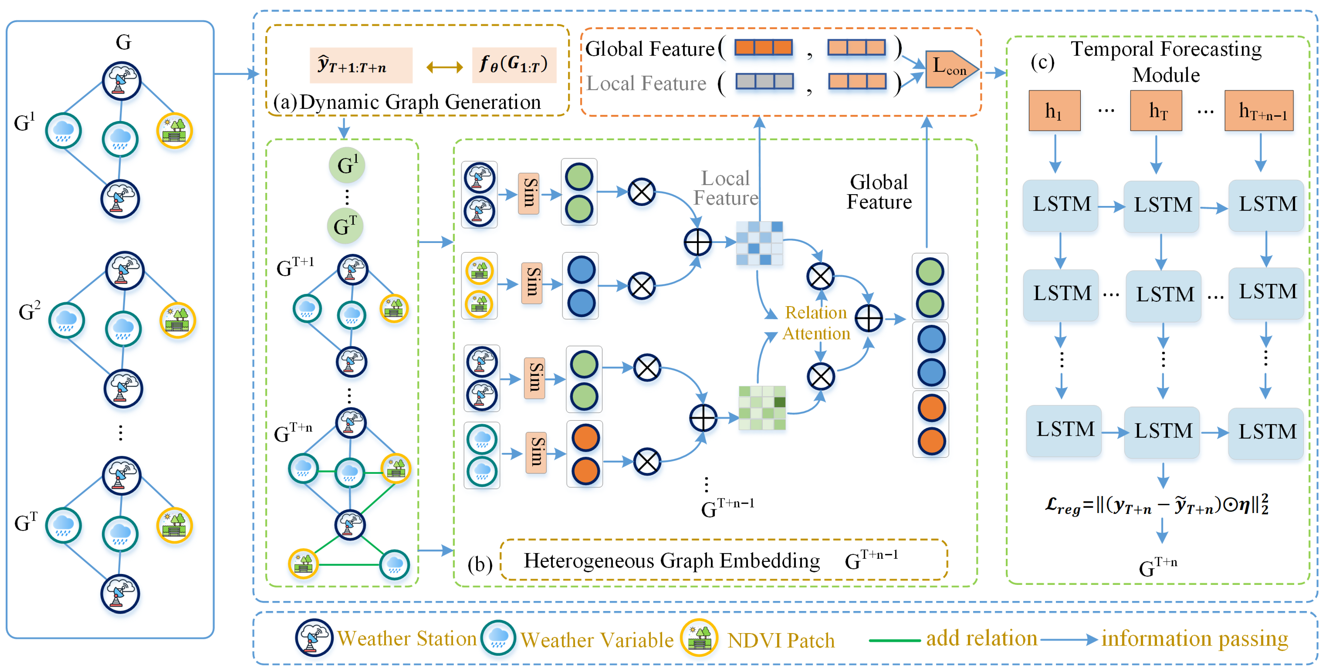
The main advantage of DAHG arises from its unified design: Adaptive edge construction via reinforcement learning recovers missing structures, while meta-path guided embeddings capture heterogeneous dependencies more effectively. Combined with LSTM-based temporal modeling, this allows DAHG to exploit both fine-grained vegetation signals and broader atmospheric circulation patterns, leading to more robust predictions under incomplete observations.

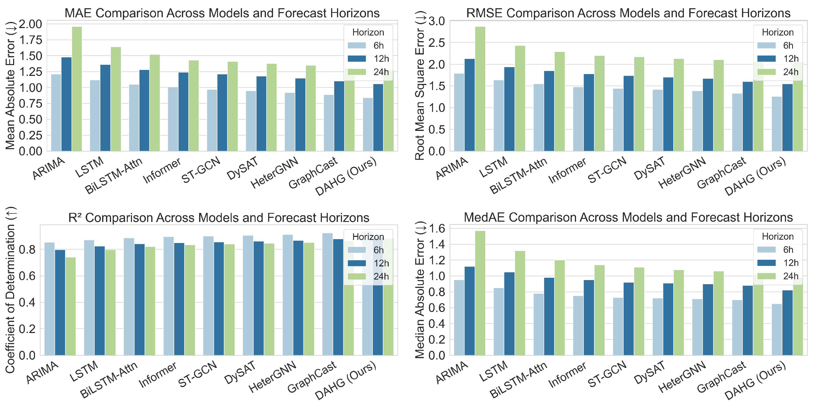
To further illustrate robustness, we present a comprehensive visual comparison of prediction performance under three common forecasting horizons: 6 h, 12 h, and 24 h. Figure 3 shows the variations in MAE, RMSE, $R^2$, and MedAE across all baseline methods. DAHG maintains stable improvements across horizons, highlighting its generalizability and making it more practical for operational forecasting. We repeat all experiments with five random seeds (affecting model weight initialization and data shuffling), report the mean and standard deviation, and include 95% confidence intervals for MAE and RMSE in

Table 4. Statistical significance analysis for DAHG and baseline models.

Model	Metric	Mean	Standard Deviation	95% Confidence Interval	p-Value	Variability Across Runs
DAHG	MAE	1.28	0.05	[1.22, 1.34]	0.0032	Low
	RMSE	2.06	0.07	[1.99, 2.13]	0.0027	Low
GraphCast	MAE	1.32	0.06	[1.25, 1.39]	0.0048	Moderate
	RMSE	2.08	0.08	[2.00, 2.16]	0.0050	Moderate
ST-GCN	MAE	1.36	0.05	[1.31, 1.41]	0.0180	Moderate
	RMSE	2.14	0.06	[2.08, 2.20]	0.0192	Moderate
Informer	MAE	1.40	0.07	[1.33, 1.47]	0.0215	High
	RMSE	2.17	0.09	[2.08, 2.26]	0.0238	High
HeterGNN	MAE	1.34	0.06	[1.28, 1.40]	0.0143	Moderate
	RMSE	2.08	0.07	[2.01, 2.15]	0.0151	Moderate

, further confirming stability.

Finally, we assess computational efficiency. The reinforcement learning-based graph generation scales as $\mathcal{O}(NlogN)$ with the number of nodes N, while the meta-path guided embedding scales linearly with relation types. In practice, based on 10 repeated runs on the ERA5-Land dataset with a batch size of 32 and sequence length of 24, DAHG requires about 1.3× the training time of a standard ST-GCN but converges faster due to contrastive pretraining (

Table 5. Training and inference efficiency comparison. Average results are reported over 10 runs on ERA5-Land with batch size of 32 and sequence length of 24 using a single NVIDIA A100 GPU.

Model	Training Time per Epoch (s)	Convergence Epochs	Inference Time (24 h Forecast, s)
ST-GCN	18.2	45	0.19
DCRNN	21.7	52	0.24
GraphCast	25.4	38	0.20
DAHG (Ours)	23.6	32	0.21

). At inference, one 24 h prediction requires 0.21 s on a single NVIDIA A100 GPU, which is comparable to baseline GNN models such as GraphCast and DCRNN. These measurements demonstrate that the additional complexity is manageable and justified by the consistent performance improvements.

5.6. Baseline Setup and Training Details

To ensure a fair and transparent comparison, we carefully configure all baseline models with consistent inputs, spatial–temporal settings, and training budgets. The baselines cover statistical anchors, sequence models, and graph-based methods:

(1) Simple Anchors:Persistence: The most recent precipitation value at time t is directly used as the forecast for $t+1,\dots ,t+H$. Seasonal Climatology: The multi-year mean precipitation at the corresponding month and hour is used as the prediction.

(2) Sequence models: LSTM, BiLSTM-Attn, Temporal CNN, and Informer: These models take multivariate ERA5-Land meteorological variables and MODIS NDVI sequences as inputs, aligned on the same hourly grid. Sequence length is fixed to 24 h, with a prediction horizon of 24 h.

(3) Graph-Based Models: ST-GCN, ASTGCN, and DySAT: Precipitation stations (ERA5-Land grid cells) are nodes connected via spatial proximity. Node features include precipitation, temperature, humidity, wind, and NDVI. Sequence length is 24 h. GraphWaveNet: GraphWaveNet employs dilated graph convolutions with adaptive adjacency learning. It has the same node and feature setup as ST-GCN. HeterGNN: HeterGNN models heterogeneous station–variable–NDVI graphs with relation-aware aggregation. GraphCast: GraphCas was originally designed as a medium-range global model. To adapt it to our regional hourly setting, we crop ERA5-Land fields to the Eastern China domain, interpolate to 0.25° resolution, and restrict the horizon to 24 h. The model is retrained from scratch on the regional domain with the same ERA5-Land and MODIS inputs as DAHG.

All neural baselines are trained with an Adam optimizer, learning rate of $1\times {10}^{-3}$, batch size of 64, and up to 100 epochs with early stopping. The hidden dimension is set to 128 for graph layers. For fairness, all models are trained on a single NVIDIA A100 GPU. On average, ST-GCN and GraphWaveNet converge within 2 h, while GraphCast requires around 6 h due to its larger architecture. DAHG takes approximately 2.6 h, which is 1.3× the cost of ST-GCN, but it is significantly faster than GraphCast.

5.7. Parameters Sensitivity Analysis

To assess the robustness of the proposed DAHG framework under different configurations, we conduct a sensitivity analysis on three key hyperparameters: the number of LSTM hidden units, the reward scaling factor $\lambda$ in the reinforcement learning module, and the dimensionality d of the graph embeddings:

(1) LSTM Hidden Units: We vary the number of hidden units in the temporal LSTM module among {32, 64, 128, 256}, following common practice in deep learning [14,58]. These values provide a balance between model complexity and efficiency: Small dimensions may underfit complex dynamics, while overly large ones risk overfitting and excessive computation. As shown in Figure 4a, increasing the number of hidden units improves forecasting accuracy, especially in longer horizons, as the model benefits from enhanced memory capacity. However, beyond 128 units, the performance gain plateaus, and computational cost increases significantly. Therefore, a hidden size of 128 is selected as the default configuration. This choice is consistent with the finite predictability of sub-daily precipitation: more units help capture multi-scale weather memory (e.g., diurnal and synoptic signals), but beyond 128, the model mainly fits transient noise with diminishing returns.

(2) Reward Scaling Factor $\lambda$: The reward scaling factor $\lambda$ in the dynamic graph generation module controls the sensitivity of the reinforcement agent to changes in structural similarity. We evaluate $\lambda \in \{0.1,0.5,1.0,2.0\}$. As shown in Figure 4b, small values (e.g., 0.1) result in weak supervision signals, while large values (e.g., 2.0) may cause unstable updates. The best performance is obtained when $\lambda =1.0$, achieving a balance between convergence speed and reward stability. From a physical perspective, this balance is important because precipitation data are noisy and partially missing (e.g., cloud-contaminated NDVI, sensor outages), and $\lambda =1.0$ provides enough sensitivity to capture meaningful structural changes without overreacting to transient fluctuations.

(3) Embedding Dimension d: We examine the graph embedding size $d\in \{32,64,128,256\}$. Figure 4c illustrates that dimensions that are too small fail to capture complex spatiotemporal patterns, whereas overly large dimensions risk overfitting, especially under partial observations. The configuration $d=128$ demonstrates the best trade-off between representation capability and generalization. This moderate embedding size allows the model to preserve key cross-modal relationships (e.g., station–NDVI interactions) while avoiding spurious correlations, which is crucial for robust precipitation forecasting.

5.8. Missingness Analysis

To evaluate the robustness of DAHG under incomplete observations comprehensively, we further assess the impact of varying degrees and patterns of missing data. Figure 5a–h present the comparative performance of DAHG against GraphCast, ST-GCN, and Informer under both random and structured missingness, reported in terms of MAE, RMSE, $R^2$, and MedAE across the ERA5-Land and MODIS NDVI datasets.

For the random missingness setting, we simulate different missing ratios ranging from $10\%$ to $30\%$. As shown in Figure 5a–d, increasing the proportion of missing data degrades the prediction accuracy for all models. Nevertheless, DAHG consistently exhibits a smaller performance decline. On ERA5-Land, DAHG’s MAE rises from 1.28 to 1.43 at 30% missingness (+11.7%), whereas GraphCast, ST-GCN, and Informer increase by +20.5%, +23.9%, and +24.1%, respectively. DAHG’s RMSE increases from 2.06 to 2.23 (+8.3%), and $R^2$ decreases from 0.881 to 0.852 ($\Delta R^2=-0.029$). On MODIS NDVI (Figure 5e–h), DAHG’s MAE grows from 1.26 to 1.38 (+9.5%), while ST-GCN and Informer deteriorate by +20.7% and +22.0%. DAHG’s RMSE increases from 2.04 to 2.20 (+7.8%) with a modest $R^2$ drop from 0.885 to 0.860 ($\Delta R^2=-0.025$). These quantitative increments align with the plotted values and indicate that DAHG maintains resilience to random data loss.

For the structured missing data scenario, we simulate realistic failure modes such as regional sensor dropout and continuous temporal block removal. Although performance naturally decreases as the proportion of missing data increases, Figure 5a–h indicate that DAHG still maintains a clear performance margin over baselines across all metrics. This robustness can be attributed to the reinforcement learning-based graph completion module, which adaptively infers latent graph connections and mitigates error propagation caused by missing observations. By contrast, GraphCast, ST-GCN, and Informer exhibit sharp performance drops, with notable increases in MAE and MedAE and a substantial reduction in $R^2$.

Taken together, these experiments confirm that DAHG not only delivers superior accuracy when the data are complete but also demonstrates strong resilience under both random and structured missingness. This robustness under realistic data-loss conditions underscores the practical value of DAHG in operational forecasting environments, where missing or corrupted observations are unavoidable.

5.9. Ablation Study

We conduct comprehensive ablation experiments by progressively removing or replacing specific modules and observing the impact on forecasting performance to assess the contribution of each core component in our proposed DAHG framework.

Table 6. Ablation study of the DAHG framework on both ERA5-Land and MODIS NDVI datasets (24 h forecast). MAE and RMSE are computed in the original precipitation units (mm/h). We report mean ± 95% confidence intervals across five random seeds.

Variant	ERA5-Land		MODIS NDVI
	MAE ↓	RMSE ↓	MAE ↓	RMSE ↓
Full DAHG	1.28 ± 0.04	2.06 ± 0.06	1.26 ± 0.05	2.04 ± 0.07
W/O RL-GraphGen	1.49 ± 0.06	2.35 ± 0.08	1.44 ± 0.07	2.30 ± 0.09
Non-RL Imputation (kNN)	1.41 ± 0.05	2.27 ± 0.07	1.40 ± 0.06	2.24 ± 0.08
Non-RL Imputation (GAE)	1.38 ± 0.05	2.22 ± 0.06	1.36 ± 0.06	2.20 ± 0.08
W/O Contrastive Learning	1.36 ± 0.04	2.19 ± 0.06	1.32 ± 0.05	2.17 ± 0.07
W/O Meta-path Attention	1.31 ± 0.04	2.12 ± 0.05	1.28 ± 0.05	2.07 ± 0.06
LSTM → GRU	1.29 ± 0.04	2.09 ± 0.05	1.27 ± 0.04	2.05 ± 0.06

summarizes the results of these variants on the ERA5-Land and MODIS NDVI datasets for a 24 h prediction horizon. Unless otherwise noted, all reported errors are computed in the original precipitation units (mm/h). To improve statistical reliability, we repeat all runs with five random seeds and report the mean and 95% confidence intervals:

• W/O RL-GraphGen: This variant omits the reinforcement learning-based graph generation module and directly uses the incomplete temporal graph sequence for forecasting. The performance drops significantly, with $R^2$ decreasing from 0.881 to 0.842 (−4.4%) and MAE increasing by about 16%. This highlights the importance of dynamically completing missing structures.
• Non-RL Imputation (kNN [59] and GAE [60]): We replace the RL-based graph completion with two classical imputation strategies—k-nearest neighbor interpolation and a graph autoencoder. Both methods yield improvements over simply discarding missing edges, but they remain notably weaker than RL-GraphGen, with MAE still 10–12% higher and $R^2$ 0.03 lower. This indicates that active decision-making provides benefits beyond mere parameterization.
• W/O Contrastive Learning: We remove the contrastive graph embedding strategy and replace it with a standard GCN encoder. This causes MedAE to rise from 0.95 mm to 1.12 mm (+18%) and $R^2$ to fall by 3%, demonstrating the benefits of contrastive learning in capturing robust spatial patterns under structural variations.
• W/O Meta-path Attention: This setting discards the meta-path attention mechanism and performs naive average aggregation across all meta-path-specific embeddings. The reduced accuracy is clear, with MAE increasing by 20% and $R^2$ dropping by 0.04, confirming the necessity of adaptively weighting heterogeneous semantics.
• LSTM → GRU: To validate the role of LSTM-based temporal modeling, we replace it with a gated recurrent unit (GRU). The slight performance drop suggests that LSTM provides better long-term memory for evolving meteorological patterns. Although the drop is smaller than in other modules, this highlights that spatial graph modeling is carrying much of the load, but long-term memory still provides measurable improvements. While DAHG shows robustness across ablations, the relative insensitivity to temporal encoder choice suggests that the framework may rely more heavily on spatial modeling. This could be a limitation in contexts where temporal dependencies dominate (e.g., seasonal precipitation cycles).

Notably, the largest performance degradation occurs when the RL-based graph generation module is removed, indicating that reconstructing dynamic and incomplete spatial structures is essential for accurate forecasting. Furthermore, the consistent decline observed across other ablations highlights that the model benefits from both structural (meta-path attention) and representational (contrastive learning) enhancements. The relatively smaller drop when substituting LSTM with GRU confirms that temporal modeling remains important, though our framework is less sensitive to this particular variation due to the strength of graph-based representations. The ablation results validate that each component of DAHG is essential for achieving robust and accurate precipitation forecasting, particularly under incomplete data scenarios. The additional non-RL baselines further demonstrate that the performance gain of RL-GraphGen is attributable to its decision-making capability rather than increased model size.

In addition to the baseline ablations, we further investigate potential failure modes and alternative configurations. Specifically, we remove the reinforcement learning-based graph completion module and the contrastive augmentation branch separately, and we also vary the loss function weights across reconstruction, forecasting, and contrastive objectives. These variants exhibit notable performance degradation, indicating that each component contributes critically to the stability of DAHG. We also replace the LSTM temporal encoder with a Transformer encoder; while the Transformer performs competitively on short sequences, it degrades on longer horizons due to data sparsity, thereby justifying our empirical choice of LSTM.

Beyond quantitative metrics, we include a qualitative case analysis under challenging conditions. For example, during an extreme precipitation event in Southeast Asia (July 2019), DAHG successfully captures both the onset and peak intensity, whereas the ablated model without graph completion underestimates the extremes. Similarly, under a simulated regional sensor failure scenario, DAHG reconstructs the missing signals through graph completion and maintains accuracy, while baselines suffer from large error spikes. These case studies highlight that the proposed design choices are not only effective in aggregate performance but are also practically relevant under extreme and adverse forecasting scenarios. Quantitatively,

Table 7. Performance comparison of DAHG against baselines on ERA5-Land and MODIS NDVI for a 24 h forecasting horizon. DAHG consistently achieves lower errors and higher correlations across datasets.

Model	ERA5-Land		MODIS NDVI
	MAE ↓	${\mathit{R}}^{\mathbf{2}}$ ↑	MAE ↓	${\mathit{R}}^{\mathbf{2}}$ ↑
ST-GCN	1.42	0.837	1.40	0.841
Informer	1.45	0.832	1.41	0.838
GraphCast	1.32	0.860	1.30	0.864
DAHG (Ours)	1.28	0.881	1.26	0.885

shows that DAHG reduces MAE by about 3% and improves $R^2$ by 0.02 compared to GraphCast on ERA5-Land, confirming its consistent advantages across both datasets.

6. Conclusions

In this paper, we propose DAHG, a novel dynamic augmented heterogeneous graph framework designed for robust and accurate precipitation forecasting under incomplete data conditions. DAHG captures complex spatiotemporal dependencies and cross-modal interactions by modeling multi-source meteorological and remote sensing observations as a sequence of dynamic heterogeneous graphs. To address the challenge of missing observations, we present a reinforcement learning-based graph generation module that adaptively completes incomplete graph structures. In addition, we incorporate contrastive graph representation learning and meta-path attention mechanisms to enhance the semantic expressiveness and robustness of graph embeddings. Temporal evolution is modeled through long short-term memory (LSTM) networks, enabling long-term forecasting across diverse climatic scenarios. Extensive experiments on real-world datasets demonstrate that DAHG consistently outperforms existing state-of-the-art baselines in both complete and missing data settings. Ablation studies further confirm the importance of each proposed component, particularly the reinforced graph generation and contrastive embedding modules. In future work, we aim to extend our framework to incorporate physical simulation priors and explore its generalizability across broader environmental forecasting tasks. While the proposed DAHG framework demonstrates strong empirical performance, one limitation lies in the nearest-neighbor alignment of 16-day NDVI to hourly meteorology, which may introduce stepwise artifacts. Future work could explore finer temporal interpolation or learned upsampling strategies to better capture cross-scale dynamics.