Classifying Protein-DNA/RNA Interactions Using Interpolation-Based Encoding and Highlighting Physicochemical Properties via Machine Learning

Abstract

Protein–DNA and protein–RNA interactions are central to gene regulation and genetic disease, yet experimental identification remains costly and complex. Machine learning (ML) offers an efficient alternative, though challenges persist in representing protein sequences due to residue variability, dimensionality issues, and the risk of losing biological context. Traditional approaches such as k-mer counting or neural network encodings provide standardized sequence representations but often demand high computational resources and may obscure functional information. To address these limitations, a novel encoding method based on interpolation of physicochemical properties (PCPs) is introduced. Discrete PCPs values are transformed into continuous functions using logarithmic enhancement, highlighting residues that contribute most to nucleic acid interactions while preserving biological relevance across variable sequence lengths. Statistical features extracted from the resulting spectra via Tsfresh are then used for binary classification of DNA- and RNA-binding proteins. Six classifiers were evaluated, and the proposed method achieved up to 99% accuracy, precision, recall, and F1 score when amino acid highlighting was applied, compared with 66% without highlighting. Benchmarking against k-mer and neural network approaches confirmed superior efficiency and reliability, underscoring the potential of this method for protein interaction prediction. Our framework may be extended to multiclass problems and applied to the study of protein variants, offering a scalable tool for broader protein interaction prediction.

1. Introduction

The interactions of biological molecules develop important functions in all species. Deoxyribonucleic acid (DNA) and ribonucleic acid (RNA) are fundamental molecules for life. DNA contains genetic information that determines the characteristics of living organisms, while RNA acts as an intermediary between DNA and proteins, carrying genetic information from the nucleus to the cytoplasm, where proteins are synthesized. The function of DNA and RNA can depend on its interaction with different proteins that allow them to perform many biological functions [1].

In the case of DNA, proteins that interact with it usually present basic residues such as arginine (R) and lysine (K) on their surface. These amino acids can form hydrogen bonds with phosphate groups and nitrogenous bases of DNA [2,3,4]. In some cases, such interactions can result in the deformation of the molecule, where the protein binds to DNA and exerts physical forces, which consequently can influence gene expression. In contrast, RNA tends to interact with protein residues that are different from those found in DNA interactions. In RNA, amino acids such as asparagine (N), serine (S), and threonine (T) can form hydrogen bonds with the phosphate and ribose groups. Tyrosine (Y) has also been observed to participate in such interactions [5,6] and this process may involve the stabilization of the secondary and tertiary structures of RNA. Consequently, protein interactions with DNA or RNA are essential for gene expression, DNA replication and repair, protein synthesis, and many other cellular functions.

The functions that proteins perform can be varied and complex to recreate in real life, where situations such as sample contamination, selection of target proteins, and classification characteristics involve high economic costs. Therefore, computational algorithms have become essential in these tasks, with the classification of protein interactions becoming a field of growing interest. Machine learning (ML) and Deep learning (DL) techniques have become increasingly important for drug discovery [7], gene expression analysis [8], the prediction of binding proteins—individual proteins that specifically interact with other molecules like DNA or RNA [9,10]—and the prediction of protein complexes, which are stable assemblies formed by multiple interacting proteins that perform a joint biological function [11]. Various types of information can be processed by Machine Learning Models (MLMs) [12,13,14,15]; as an example, they can learn about text strings using natural language processing (NLP), which is applicable to proteins since they are usually encoded in FASTA format, the most common protein encoding format, which is represented in plain text [16]. A NLP approach can be used to learn information from text data sources. However, NLP is not suitable for protein analysis when data sets are small or the sequence sizes are not homogeneous [17]. While FASTA is an efficient way to represent proteins, its use in MLMs poses a variety of inherent challenges to ML and presents diverse opportunities to enrich the sequence information.

In order to implement MLMs training, an encoding process is required that transforms the text sequences into a representation containing the same number of predictors for each protein [18]. One-hot encoding is an example of this type of encoding [19]. This method transforms each protein into a numeric matrix, which changes the dimensions of the original data. A further bioinformatics technique is matrix encoding with k-mer counting, which can be used to analyze proteins and identify genotypes [20]. Specifically, the naïve approach to counting k-mer involves overlapping a set of residues in each protein to build a dictionary of words and then counting each occurrence within each protein sequence, resulting in a representative matrix with numeric values. Despite this, matrix-based encoding significantly increases memory requirements for each input. In the case of one-hot encoding, zeros and ones are used to represent the entire data set, making it difficult to separate samples and losing biological references such as residue positions [21].

The positions where amino acids are present in proteins are of significant importance. It is known that the position of amino acids are related to domains or motifs, which are regions of biological relevance in a protein [22]. However, when amino acid encoding is applied, the positional reference of these regions is lost. Consequently, the biological origin of a protein sequence is altered, which directly affects when it is desired to classify its protein function. In order to accurately differentiate between protein classes or functions, it is necessary to include well-known information on protein sequences that respond well to encoding. According to some reports, specific amino acids are more likely to be present in certain interactions (protein–DNA/RNA), making them suitable candidates for use in protein sequence encoding [2,3,5,6].

There are several approaches that can be used to integrate additional information on proteins for this purpose. For instance, Mckenna et al. [23] incorporated amino acid sequence spectra information with protein structural and physiochemical descriptors to classify molecular activities. However, selecting amino acid features is more complex when considering an encoding. To illustrate this point, Chen et al. [24] developed a scaling matrix based on standardized protein lengths for each amino acid, encoding two pairs of $<P_i,P_j>$ proteins using two lowest common ancestor (LCA)-derived feature vectors of each pair, thereby indicating gene ontology hierarchy. A more complex model is the alpha-fold model [25], which incorporates amino acid distance matrices, atom positions, and physicochemical properties (PCPs) into a convolutional neural network (CNN) to predict 3D structure folding.

In addition to the encoding problem, we can find different models such as Multilayer Perceptron (MLP), Convolutional Neural Networks (CNNs), Long-short term memory (LSTM), ensemble models, or even novel architectures to solve protein classification [9,26,27]. However, the treatment of protein information produced by these methods can be difficult to interpret in relation to a desired biological context [17]. Alternatively, classical methods are used to distinguish between protein interactions, including SVM [28], k-NN [29], DT [30], RF [31], GNB [32], and MLP [33], which evaluate whether predictors contribute to separate classes or not. In this regard, an adequate representation of proteins (encoding) is essential to train different classifiers and to obtain accurate performance metrics in each model.

On the other hand, it is important to define the universe of proteins to be classified, since a single cell can contain millions of proteins [34]. Therefore, the reduction of protein sequence data sets is considered a limitation of MLMs training. A possible solution would be to obtain unbalanced data sets with fewer occurrences of selected proteins, which would have implications for experimental design [35]. Consequently, even when the data set is small, it is necessary to extract as much information (features) for each protein to improve the training of the ML algorithms.

Thus, the main challenge would be to obtain a numerical representation of the protein sequences, which implies biological features and an adequate contextualization of the protein residues, since the type of information provided to the learning algorithms is crucial to find the separability of the classes. For example, it has been reported that DNA sequences can be represented numerically by one-dimensional vectors, which are a viable representation to extract a characteristic signal [36]. Therefore, continuous representation encoding is a promising method for recording contextual information on other macromolecules of biological interest [37]. This is most likely the case for proteins, which are mainly composed of amino acids and possess a variety of PCPs such as polarity, hydrophobicity, etc. which contribute to the interaction with the two macromolecules essential to living organisms (DNA and RNA).

Unfortunately, the problem of dimensionality persists, even with the substitution of amino acids by numerical values that will be represented by a characteristic function obtained from the physicochemical properties of the amino acids that make up the protein sequence. The length of the different protein sequences must be the same for the entire data set to generate a good characteristics extraction process. One solution to normalize the sequence length is through polynomial interpolation of the physicochemical properties of proteins. This is a simple technique to fit a function with a discrete set of points to find intermediate information between known numerical values. More precisely, it is a non-parametric function that generates an interpolated curve, based on given inputs, using low-degree polynomials [38,39]. This continuous function can be obtained for a desired number of amino acids by considering their respective physicochemical properties, thus producing dimensional consistent representations of protein sequences that can then be incorporated into a learning classifier for the prediction of protein sequence interactions with DNA or RNA.

As a result of this work, we make the following major contributions:

• Use of logarithmic labeling to highlight numerical values associated with the physicochemical properties of amino acids that predominate in protein–DNA/RNA interactions.
• Continuous representation of protein residues derived by interpolating discrete values relating to their physicochemical properties.
• Automatic feature extraction from continuous protein spectra using TSfresh (Time Series Feature extraction based on scalable hypothesis tests) Python package to feed and improve supervised binary classification (to infer protein interaction type).
• Comparison of the proposed approach based on continuous representation of protein sequences with k-mer counting, a method commonly used in bioinformatics.

The present work provides a novel framework for classifying protein affinities with DNA and RNA using a variety of machine learning algorithms (SVM, k-NN, DT, RF, GNB, and MLP), thereby enhancing both performance and interpretability.

2. Materials and Methods

2.1. Protein Dataset

We recovered 7058 human proteins from the UNIPROT [40] database using SPARQL tool [41], of which 4323 interact with DNA and 2735 with RNA. Proteins were labeled according to their Gene Ontology (GO) molecular function annotations in UniProtKB: GO:0003677 (“DNA binding”) and GO:0003723 (“RNA binding”) [42]. To ensure reliability, only annotations supported by experimental or manually curated evidence codes (e.g., EXP, IDA, IPI, IMP, IGI, IEP, and their high-throughput equivalents) were included, while automatically inferred (IEA) annotations were excluded. This approach guarantees that all binding interactions are based on experimentally supported and curator-reviewed evidence.

Since proteins are composed of a variety of amino acid residues, their lengths vary. For example, the extracted data set can include protein sequences ranging in length from 16 to 5540 amino acids. In order to exclude longer or shorter sequences, proteins whose sequences were between 55 and 800 residues were selected. In order to ensure that the data set was balanced, 2735 sequences were drawn at random from the existing DNA class using Phyton’s pseudo-random number generator [43]. A statistically significant comparison was made between the subsets of proteins that interact with DNA by selecting ten random samples from 2735 protein sequences.

2.2. Proposed Encoding with Physicochemical Properties

The FASTA format preserves the position of the amino acids (AAs) that make up the protein, and the order in which they are present can contribute to understanding the function the protein performs. This protein configuration is the basis of the encoding proposal for MLMs to perform classification. For MLMs, dimensions are needed to be the same for any input, considering text representation always implies a transformation to have the same number of predictors in the dataset.

The proposed method uses PCPs to encode proteins. These physicochemical characteristics are presented in

Table 1. Fourteen Physicochemical Properties (PCPs) numerically associated with the 20 essential amino acid residues: ${\mathrm{H}}_{11}$ & ${\mathrm{H}}_{12}$ hydrophobicity, ${\mathrm{H}}_2$ hydrophilicity, NCI net charge index of side chains, ${\mathrm{P}}_{11}$ & ${\mathrm{P}}_{12}$ polarity, ${\mathrm{P}}_2$ polarizability, SASA solvent-accessible surface area, V volume of side chains, F Flexibility, ${\mathrm{A}}_1$ Accessibility, E Exposed, T Turns, ${\mathrm{A}}_2$ Antigenic. Values extracted from Chen et al. [24].

AAs	H11	H12	H2	NCI	P11	P12	P2	SASA	V	F	A1	E	T	A2
A	0.62	2.1	−0.5	0.007	8.1	0	0.046	1.181	27.5	−1.27	0.49	15	−0.8	1.064
C	0.29	1.4	−1.0	−0.037	5.5	1.48	0.128	1.461	44.6	−1.09	0.26	5	0.83	1.412
D	−0.9	10	3	−0.024	13	40.7	0.105	1.587	40	1.42	0.78	50	1.65	0.866
E	−0.74	7.8	3	0.007	12.3	49.91	0.151	1.862	62	1.6	0.84	55	−0.92	0.851
F	1.19	−9.2	−2.5	0.038	5.2	0.35	0.29	2.228	115.5	−2.14	0.42	10	0.18	1.091
G	0.48	5.7	0	0.179	9	0	0	0.881	0	1.86	0.48	10	−0.55	0.874
H	−0.4	2.1	−0.5	−0.011	10.4	3.53	0.23	2.025	79	−0.82	0.84	56	0.11	1.105
I	1.38	−8.0	−1.8	0.022	5.2	0.15	0.186	1.81	93.5	−2.89	0.34	13	−1.53	1.152
K	−1.5	5.7	3	0.018	11.3	49.5	0.219	2.258	100	2.88	0.97	85	−1.06	0.93
L	1.06	−9.2	−1.8	0.052	4.9	0.45	0.186	1.931	93.5	−2.29	0.4	16	−1.01	1.25
M	0.64	−4.2	−1.3	0.003	5.7	1.43	0.221	2.034	94.1	−1.84	0.48	20	−1.48	0.826
N	−0.78	7	2	0.005	11.6	3.38	0.134	1.655	58.7	1.77	0.81	49	3	0.776
P	0.12	2.1	0	0.24	8	0	0.131	1.468	41.9	0.52	0.49	15	−0.8	1.064
Q	−0.85	6	0.2	0.049	10.5	3.53	0.18	1.932	80.7	1.18	0.84	56	0.11	1.015
R	−2.53	4.2	3	0.044	10.5	52	0.291	2.56	105	2.79	0.95	67	−1.15	0.873
S	−0.18	6.5	0.3	0.005	9.2	1.67	0.062	1.298	29.3	3	0.65	32	1.34	1.012
T	−0.05	5.2	−0.4	0.003	8.6	1.66	0.108	1.525	51.3	1.18	0.7	32	0.27	0.909
V	1.08	−3.7	−1.5	0.057	5.9	0.13	0.14	1.645	71.5	−1.75	0.36	14	−0.83	1.383
W	0.81	−10	−3.4	0.038	5.4	2.1	0.409	2.663	145.5	−3.78	0.51	17	−0.97	0.893
Y	0.26	−1.9	−2.3	117.3	6.2	1.61	0.298	2.368	0.024	−3.3	0.76	41	−0.29	1.161

, previously reported by Chen et al. [24]. In this table, the 20 essential AAs are characterized by 14 physicochemical properties. During the sequence curation process, Table 1 was used as reference because the protein information obtained from UNIPROT includes chains that contain non-standard residues, such as “X” (unknown amino acid) and “U” (selenocysteine), which are not part of the 20 canonical amino acids described by Chen et al. [24]. Consequently, sequences containing these residues were excluded from the final dataset to ensure descriptor consistency and comparability across all encoded proteins.

After curation, the amino acid sequences were subjected to the first phase of the proposed encoding method (see Figure 1). The process begins with the conversion of each AAs into 14 physicochemical properties. Each group of properties is a unique set of values. The organization of the properties is maintained for each AAs without altering the order shown in Table 1.

The FASTA format sequence is iterated to exchange the residues for the corresponding sets of properties. Through this process, the position of the AAs is preserved, as only the representation is swapped from a character to a vector of numerical values. This process yields a one-dimensional vector. Assuming that protein P contains N residues, the resulting encoding will have M values of physicochemical properties in the amino acid sequence of protein P defined by $N\ast 14$. Considering that the purpose of this study is to classify proteins that interact with DNA and RNA molecules, the first step we take is to identify which amino acids play a prominent role in each type of interaction. There is evidence that arginine (R), lysine (K), and glutamine (Q) are the amino acids that are likely to interact with DNA most closely [2,3,5]. In contrast, the most closely related RNA residues are Serine (S), Threonine (T), Asparagine (N), and Tyrosine (Y) [6]. This information allows us to detect the type of interaction that a protein sequence will have by assigning a certain weight to the amino acids of the sequence whose interaction we wish to determine (highlight process).

To achieve this, we applied a logarithmic function to the fourteen physicochemical properties corresponding to each residue involved in DNA and RNA interactions, allowing a more balanced comparison across amino acids with distinct biophysical scales. Although not derived from a probability test, the logarithmic scaling minimizes potential bias introduced by highly variable property distributions and facilitates the identification of meaningful variations associated with DNA- or RNA-binding residues. Prior to logarithmic enhancement, the data was normalized in the range of 0.00000001 to 100, in order to avoid negative logarithms.

2.3. Cubic B-Spline Interpolation

A polynomial interpolation refers to the construction of a curve that crosses a set of given points using a low-degree polynomial function. If the segments between these points are smooth and piecewise, this type of interpolation is called Spline [39,44]. In this work, we used a cubic B-spline curve S(t) defined by four control points P0, P1, P2, and P3 over the normalized knot interval t ∈ [0,1]. Consequently, it can be expressed as a polynomial of degree 3:

$$S(t)=\sum _{i=0}^3{G}_{i,4}(t)\ast P_i$$

(1)

where $G_{i,4}(t)$ are basis cubic functions known as B-spline polynomials for curve segment S(t), which are defined by:

$$\begin{array}{cc}\hfill G_{0,4}(t)& ={\displaystyle \frac{1}{6}}(1-3t+3t^2-t^3)\hfill \\ \hfill G_{1,4}(t)& ={\displaystyle \frac{1}{6}}(4-6t+3t^3)\hfill \\ \hfill G_{2,4}(t)& ={\displaystyle \frac{1}{6}}(1+3t+3t^2-3t^3)\hfill \\ \hfill G_{3,4}(t)& ={\displaystyle \frac{1}{6}}(t^3)\hfill \end{array}$$

Cubic B-spline interpolation produces differentiable functions from control points (numerical values) to generate smooth cubic curves. This study used numerical values associated with physicochemical properties of amino acids to classify 5470 protein sequences based on their interactions with DNA and RNA. The functions obtained through spline interpolation are used to achieve different sampling sizes depending on the desired precision level. Thus, the more points that are provided to the function, the more defined the result will be.

Since all proteins are now represented by functions with the same number of points, all sequences contain the same amount of information regardless of the initial number of amino acids. A further consideration when presenting this representation is the range within which the encoding is presented. A range was adapted which contained all encoded values in order to maintain consistency between encoded proteins. That is, all M values of each protein were placed within the range of 0 to $b-1$. By adjusting the points to this range, we can ensure that the sampling can be conducted at the same frequency in all cases.

For each protein, the interpolation is generated using this series of points. The position of the PCPs is initialized at zero in order to maintain consistency with discrete time, as would be done with discrete signals. As a result, the sampling range is defined as follows:

$$[a,b-1]=\left\{x\in \mathbb{R}|a\le x_1,x_2,\dots ,x_M\le b-1\right\}$$

(2)

where

• a = 0
• b = Highest value in selected range.
• $x_1$, $x_2$, …, $x_M$ = M consecutive positions for encoded values.

Using interpolation, intermediate information is obtained which is used to generate a unique function which passes through the points corresponding to the physicochemical properties. For each protein, a different function will be assigned, and these functions are used to estimate values depending on the number of samples required. For consistency, all functions characterizing proteins must return the same number of samples, ensuring that encoded proteins have the same amount of information. As more samples are obtained, the better the information will be characterized as compared to the original data; otherwise, the function will provide estimated results, which may omit segments of the signal. Encoded proteins are fitted using the same sampling rate with R samples for congruence. To simplify process of approximation by interpolated representation, we define that, a number of samples to evaluate the interpolation is equal to b, this new evaluation range can be written as:

$$[a,b]=\left\{x\in \mathbb{Z}|a\le y_1,y_2,\dots ,y_R\le b\right\}$$

(3)

$y_1$, $y_2$, …, $y_R$ are R consecutive samples equally distributed.

For this study, we consider four different window sizes for the interpolated function (which we will refer to as the protein signal); 512, 1024, 2048, and 4096 samples.

2.4. Feature Extraction and Selection

We used an open-source Python package called Tsfresh (Time Series Feature Extraction based on Scalable Hypothesis Tests) [45] to extract all the features from the spline interpolation (protein signal). To prepare protein signals for Tsfresh, we arrange them in sequences of successive windows, moving from 0 to b − 1 in time-varying steps through the protein’s interpolated points. Tsfresh extracted 788 features from each of the four window sizes (512, 1024, 2048, and 4096 samples) of the interpolated function. Feature sets for each window size were reduced by removing repeated features to eliminate redundancy, leaving only the relevant features as shown in

Table 2. Number of extracted features.

Samples	Original Features	Relevant Features
512	788	24
1024	788	152
2048	788	163
4096	788	178

. The extracted features are used as inputs for MLMs, as is presented in Figure 2.

2.5. Classifiers for Spline Interpolated Features

Six Machine Learning classifiers (SVM, k-NN, DT, RF, GNB, and MLP) were trained to determine the protein-ADN/RNA interaction using the most relevant features obtained from Tsfresh. From the extracted features, two sets of data were taken: 25% for testing and 75% for training.

2.5.1. Decision Tree (DT)

Decision tree (DT) models are simple if-then rule supervised classifiers that can classify input data based on a range of values. DT is useful for stratifying data by learning decision rules based on the data features [46]. Here, we used the DT model provided by the python package scikit-learn (version 1.1.2) in order to construct our binary classifier (protein binding to DNA or RNA). Hyperparameters were set to all default values. The way in which decision trees works resembles typical decisions of experts on separability of information. As we work with proteins labeled by experts, its relevant to compare outputs of this algorithm.

2.5.2. Support Vector Machine (SVM)

Support Vector Machine (SVM) classifiers are supervised machine learning algorithms that are used to identify boundaries within input spaces. The SVM model is trained with the input features in order to produce non-linear function. An SVM model is a suitable algorithm for problems in which the input data can be separated between classes using an optimal hyperplane. However, the inputs contain a large feature space. or this study, two classes of protein interactions were considered: (1) Protein interaction with DNA and (2) Protein interaction with RNA, and both were calculated using the SVC method of the scikit-learn package (version 1.1.2) [47], the SVM algorithm is suitable for analyzing protein interactions in order to determine the feasibility of separating proteins into classes. SVMs separate classes by solving a minimization problem defined as follows:

$${\displaystyle \frac{1}{2}}{w}^{T}w+C\sum _{i=1}^N{\xi }_i$$

(4)

subject to:

$$\begin{array}{c}\hfill y_i(w^T{x}_i+b)\le 1-{\xi }_i\end{array}$$

where,

$$\begin{array}{c}\hfill {\xi }_i\ge 0\end{array}$$

training vectors are $x_i\in {\mathbb{R}}^{\mathbb{N}}$, being features extracted from proteins, with $y_i\in \left\{-1,1\right\}$ being the respective classes. Variable i goes from 1 to N and represents the number of proteins in the dataset. A normal vector perpendicular to the separation hyperplane is represented with w, and ${\xi }_i$ are slake variables for manage an error range in classification. A cost parameter C is introduced to set a trade-off between the margin and training error.

2.5.3. K-Nearest Neighbors

The K-Nearest Neighbors (k-NN) algorithm is a classification technique used in supervised machine learning to predict features spatially (via distances). The k-NN classifier identifies the closest neighbors based on the Euclidean distance between them and assigns the class label that is favored between these neighbors to the test data point [48]. In the K-NN algorithm, the Euclidean distance metric is expressed as follows:

$$d(x_i,x_j)=\sqrt{\sum _{r=1}^p{(x_{ri}-x_{rj})}^2}$$

(5)

The k-NN formula calculates the Euclidean distance between inputs, in this case proteins. $x_i$ and $x_j$ represent different proteins to calculate. In this case, p represents the number of predictors or features for proteins. Distances between them are calculated for every case, and a class is assigned to each protein. For this study, the k-NN model was implemented using the KNeighborsClassifier from sklearn (version 1.1.2).

2.5.4. Random Forest

The Random Forest Classifier (RF) is a collective learning method that uses numerous decision trees (DT) to reduce overfitting. In each tree, a random subset of features and training data is generated [49]. The algorithm output is the average class classification of all the trees in the forest. In this work, a RF classifier was implemented in Python using the Scikit-Learn (sklearn, version 1.1.2) library with the RandomForestClassifier function.

2.5.5. Gaussian Naive Bayes

Gaussian Naive Bayes (GNB) is an ML classifier that uses the normal probability distribution of input data to infer class labels. Probabilities from each feature are combined to determine if the data belongs to a specific class, and higher probabilities indicate a better classification. Assuming that each feature follows a normal distribution, the probability that a protein signal belongs to one of the classes (interacting with DNA or RNA) can be expressed as follows:

$$P(x_i|y)={\displaystyle \frac{1}{\sqrt{2\pi {\sigma }_y^2}}}(e^{-}{\displaystyle \frac{{(x_i-{\mu }_y)}^2}{2{\sigma }_y^2}})$$

(6)

where,

• ${\mu }_y$ is mean
• ${\sigma }_y^2$ is standard deviation

2.5.6. Multilayer Perceptron

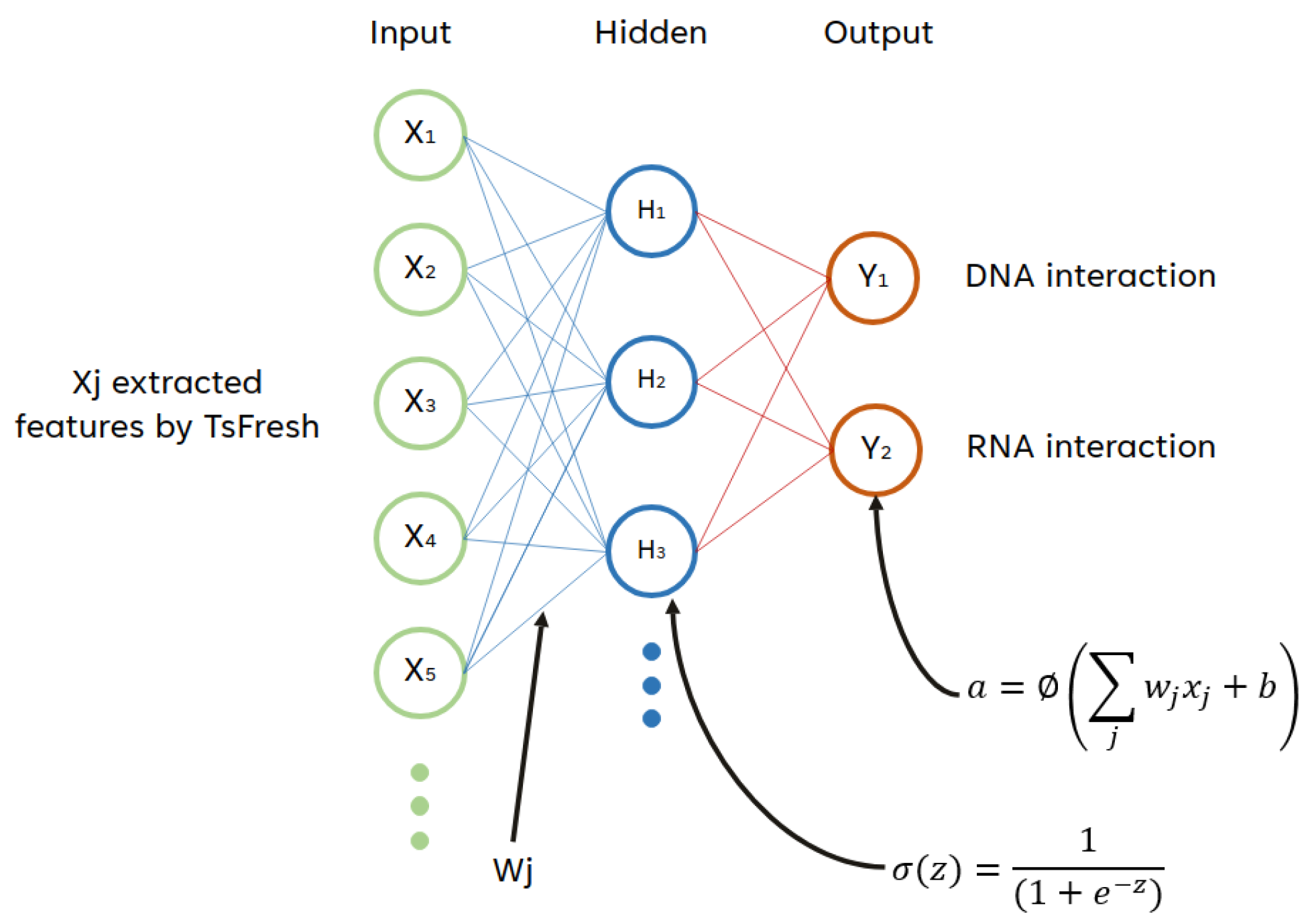
The Multi-Layer Perceptron (MLP) classifier is a supervised learning algorithm used for classification tasks, which is based on artificial neural networks composed of multiple layers, including an input layer “x”, hidden layers “h”, and an output layer “y”, where each layer contains a set of perception elements known as neurons (see Figure 3). Neurons in the forward layers are connected to each other by weights “W”, and an additional bias term “b” is provided to introduce a threshold for activation of neurons “a”. In MLP, an output is defined by Equation (7). Alternatively, the forward learning process uses the error calculation and backpropagation to adjust the weights and improve the classification defined by Equations (8) and (9).

$$y_j^h=f(\sum _{i=1}^{m_{h-1}}{W}_{ji}^h{z}_i^{h-1}+b_j^h)$$

(7)

$$w_{kl}^{h+2(New)}=w_{kl}^{h+2(Old)}+\eta {\delta }_l^{h+2}{y}_l^{h+1}$$

(8)

$${\delta }_l^{h+2}=y_l^{h+2}(1-y_l^{h+2})e$$

(9)

An MLP classifier can be useful when there is a high density of features in the input data, as is the case with interpolated protein sequences (signals). Therefore, this method was implemented with Sklearn’s MLPClassifier (version 1.1.2), using default hyperparameters. Three layers were considered: an input layer with the number of features extracted with TsFresh (24, 152, 163 and 178), a hidden layer with 100 neurons and an output layer with 2 neurons, since this is a binary classification problem.

2.6. Evaluation Metrics

The six classification models (SVM, k-NN, DT, RF, GNB, and MLP) were evaluated using the following performance metrics:

$$Accuracy={\displaystyle \frac{TP+TN}{TP+TN+FP+FN}}$$

(10)

$$Precision={\displaystyle \frac{TP}{TP+FP}}$$

(11)

$$Recall={\displaystyle \frac{TP}{TP+FN}}$$

(12)

$$F1score=2\ast {\displaystyle \frac{Precision\ast Recall}{Precision+Recall}}$$

(13)

where TP is the number of true positive outcomes (correctly classified protein–DNA/RNA interactions), TN is the number of true-negative outcomes (correctly classified protein–DNA/RNA non-interactions), FP is the number of false-positive outcomes (incorrectly classified protein–DNA/RNA non-interactions) and FN is the number of false-negative outcomes (incorrectly classified protein–DNA/RNA interactions). The mean and standard deviation of classification performance were computed in 10 repeat runs to acquire average values for balanced data sets.

3. Results

3.1. Dataset Balance Evaluation

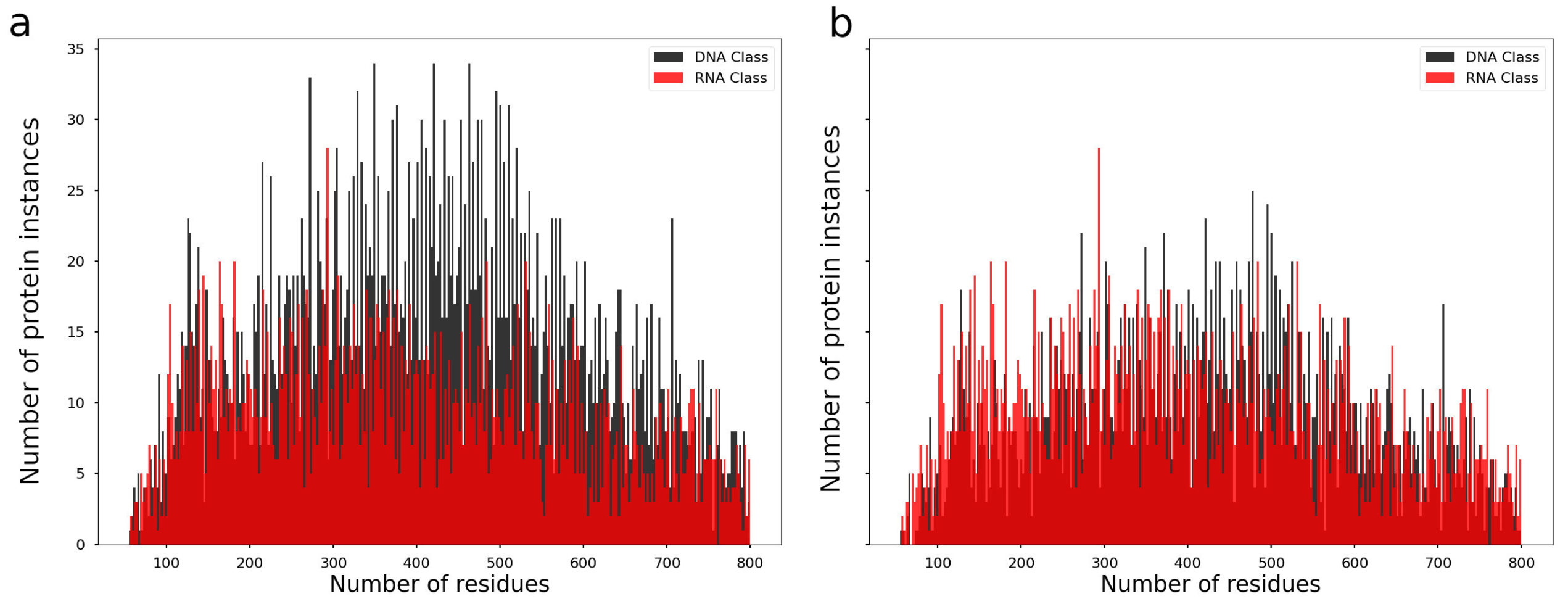
We balanced protein classes in order to avoid bias in the classification of interaction types (with DNA or RNA). For this purpose, we correlated the number of protein incidents with the amount of amino acids (residues) present in them. Figure 4a and Figure 4b show the histograms for the unbalanced and balanced datasets, respectively. Additionally, it can be seen that the distribution of residues can hold certain noise, since there are some peaks of more occurrences of specific sizes of proteins. A more comparable data set of DNA-interacting proteins was observed. However, the lengths are not fully homogeneous. For this reason, the 10 random samples were used to train and test the classifiers and establish the standard deviation of the results.

3.2. Protein Encoding

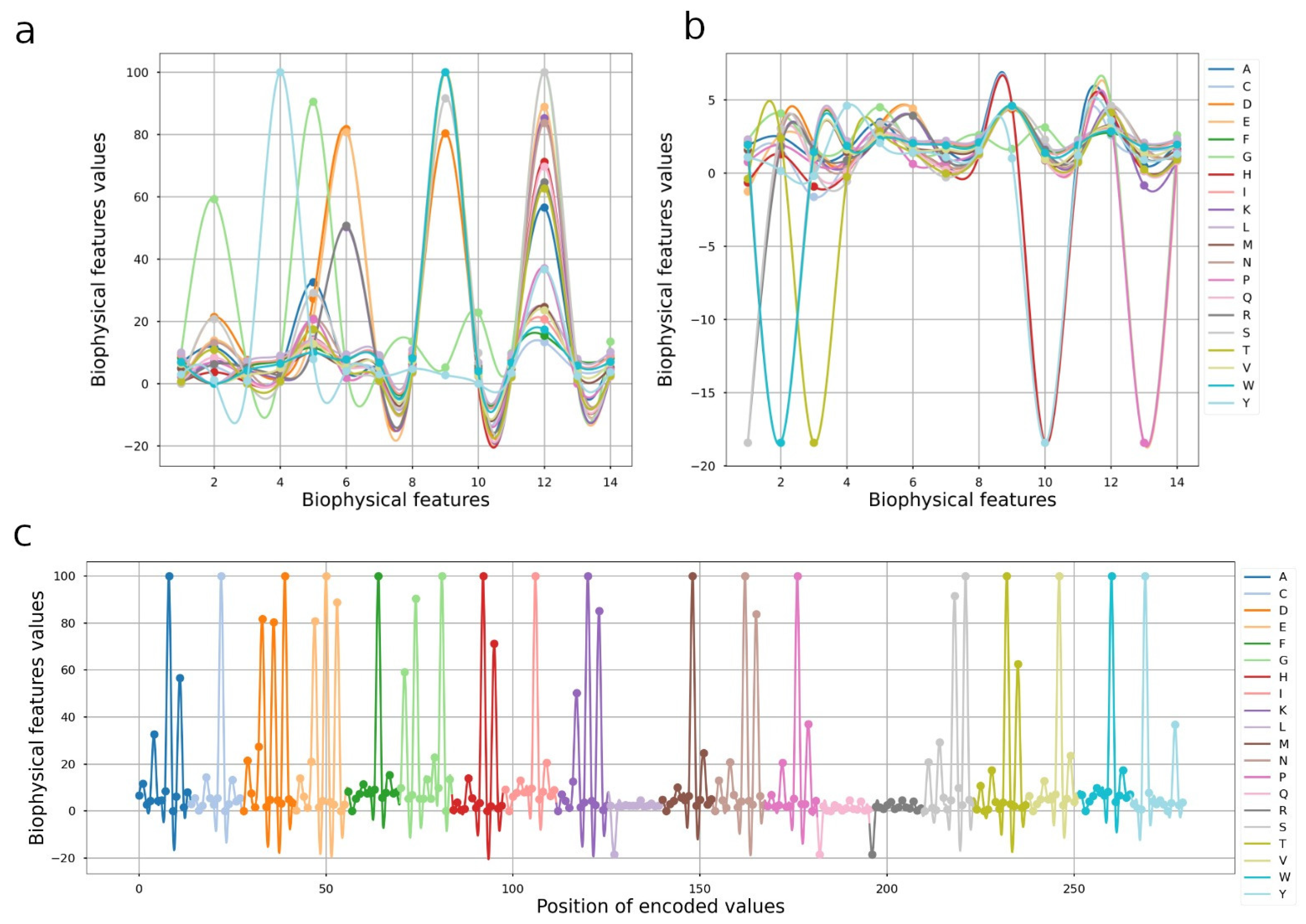
The amino acids were transformed into vectors of 14 physicochemical properties (PCPs) and concatenated in the same order as the original amino acids in the protein sequence. This concatenated representation serves as the input for generating a continuous signal via cubic B-spline interpolation. Figure 5a shows the interpolation of each of the 20 canonical amino acids using cubic B-splines. Figure 5b presents the same 20 amino acids after applying a logarithmic transformation to the PCPs, which generates a different scale and enables clearer differentiation of amino acids compared to Figure 5a. Figure 5c shows a synthetic protein sequence processed with our algorithm to identify amino acids relevant to DNA interaction, concatenated into a single sequence that includes both non-logarithmically and logarithmically transformed PCPs. Together, these three panels illustrate the encoding process with B-splines and demonstrate how the method captures a continuous representation of amino acids while preserving their relative differences.

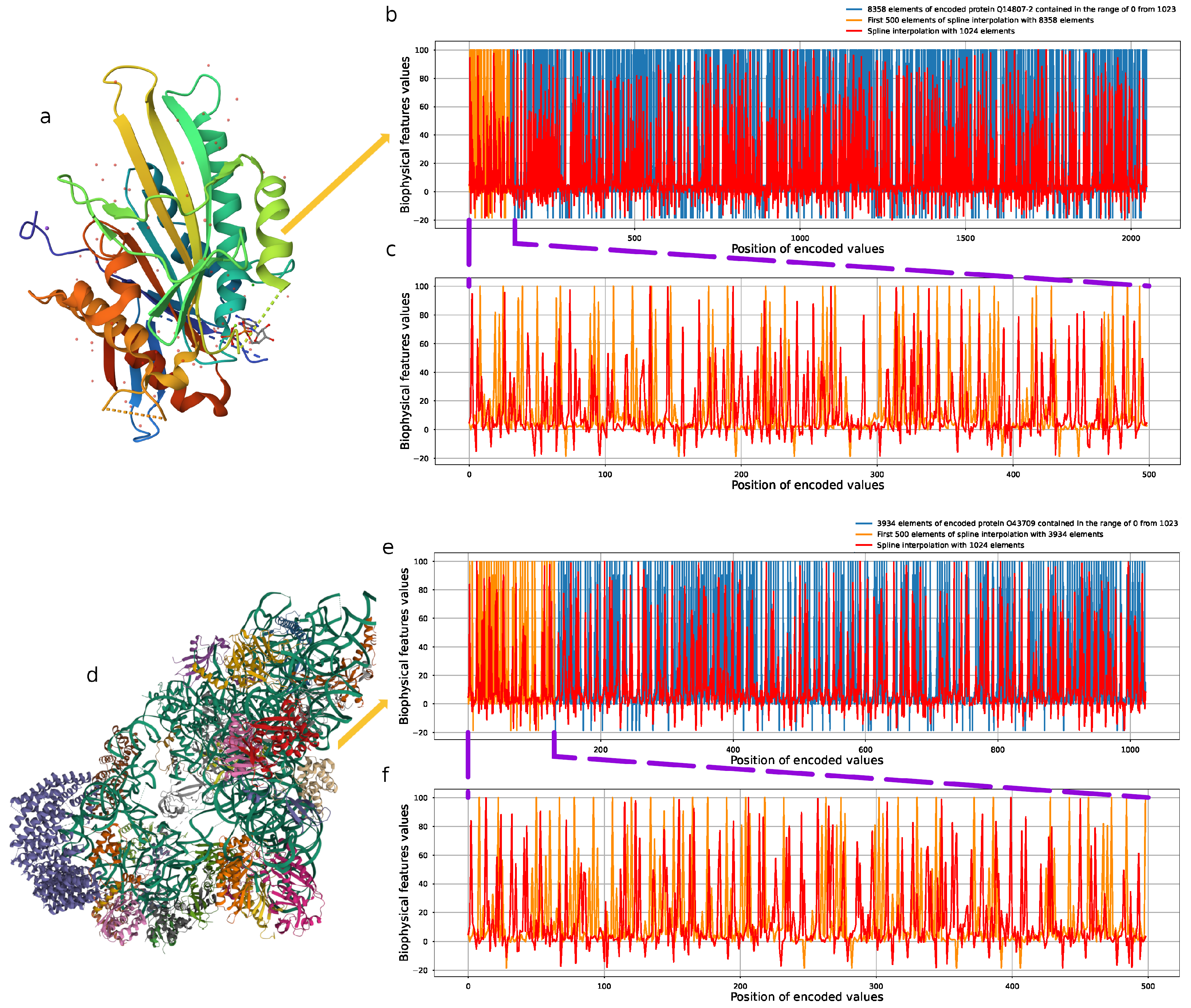
Building on this procedure, we encoded full protein sequences for both DNA- and RNA-binding proteins, standardizing all sequences to a common range of 0–1023 regardless of their original lengths. Figure 6a–c illustrate the DNA-binding protein Q14807-2, with panel (a) showing the tertiary structure, (b) the encoded signal derived from the cubic B-spline function fitted to the 14 physicochemical properties of each amino acid (blue curve: high-resolution signal with 8358 elements; red curve: downsampled signal with 1024 elements), and (c) a zoom of the first 500 elements. Similarly, Figure 6d–f depict the RNA-binding protein O43709, with panel (e) showing 3934 high-resolution samples and the 1024-point downsampled B-spline interpolation, and panel (f) a magnified view of the first 500 elements.

The B-spline encoding captures both positional and physicochemical information for each amino acid, generating characteristic vectors of length M, determined by the number of residues multiplied by the 14 properties (see Table 1). While higher sample counts improve the resolution of the encoded signal, all interpolations were resampled to 1024 points to maintain uniformity across both protein sets, producing N + 1 polynomials per protein and preserving essential biophysical information for downstream feature extraction and model training.

Figure 7 illustrates the effect of different sampling ranges (512, 1024, 2048, and 4096 samples; Figure 7a–d) on the encoded signals, sampled according to Equation (2) and fitted using Equation (3) with R set to b. The blue curve, shown as a background in all panels, represents the high-resolution signal of protein Q14807-2, while the red curves correspond to the sampled points extracted at each respective resolution. Comparing multiple sampling ranges allows us to assess how the amount of captured information affects the features extracted by TSfresh and the resulting performance of ML classifiers. Notably, the number of residues does not influence the interpolation range when values are uniformly distributed, and the cubic B-spline interpolation effectively reconstructs the original signal, with higher fidelity achieved as the number of samples increases.

The same approach was applied to the full datasets of all DNA- and RNA-binding proteins. This ensured that each protein, regardless of its sequence length, was standardized to the same range and interpolated with cubic B-splines, providing uniform, signal representations suitable for feature extraction with TSfresh and subsequent classification tasks.

3.3. Classifiers Performance

The classification results without applying the logarithmic highlight are presented in

Table 3. Classifiers Results without logarithm. Results are presented as the mean performance metrics for ten runs. The results used for the comparison are highlighted in bold.

Samples	Algorithm	Accuracy	Precision	Recall	F1 Score
512	SVM	$65.6\%\pm 0.90$	$66.2\%\pm 0.83$	$65.6\%\pm 0.90$	$65.4\%\pm 0.92$
	k-NN	$50.5\%\pm 0.98$	$50.6\%\pm 0.97$	$50.5\%\pm 0.98$	$50.5\%\pm 0.98$
	DT	$53.9\%\pm 1.12$	$54.0\%\pm 1.16$	$53.9\%\pm 1.12$	$53.8\%\pm 1.11$
	RF	$57.9\%\pm 1.20$	$58.4\%\pm 1.21$	$57.9\%\pm 1.20$	$57.8\%\pm 1.23$
	GNB	$59.6\%\pm 0.95$	$59.5\%\pm 0.97$	$59.6\%\pm 0.95$	$59.4\%\pm 0.94$
	MLP	$61.2\%\pm 0.56$	$61.3\%\pm 0.60$	$61.2\%\pm 0.56$	$61.2\%\pm 0.57$
1024	SVM	$62.4\%\pm 1.21$	$62.6\%\pm 1.17$	$62.4\%\pm 1.21$	$62.4\%\pm 1.20$
	k-NN	$52.1\%\pm 0.60$	$52.2\%\pm 0.62$	$52.1\%\pm 0.60$	$52.1\%\pm 0.60$
	DT	$52.2\%\pm 1.22$	$52.5\%\pm 1.26$	$52.2\%\pm 1.22$	$52.2\%\pm 1.22$
	RF	$54.4\%\pm 1.04$	$54.8\%\pm 1.02$	$54.4\%\pm 1.04$	$54.3\%\pm 1.07$
	GNB	$58.7\%\pm 0.89$	$58.8\%\pm 0.97$	$58.7\%\pm 0.89$	$58.0\%\pm 1.09$
	MLP	$59.2\%\pm 1.09$	$59.3\%\pm 1.04$	$59.2\%\pm 1.09$	$59.2\%\pm 1.08$
2048	SVM	$\mathbf{65.6}\%\pm \mathbf{0.90}$	$\mathbf{66.2}\%\pm \mathbf{0.83}$	$\mathbf{65.6}\%\pm \mathbf{0.90}$	$\mathbf{65.4}\%\pm \mathbf{0.92}$
	k-NN	$\mathbf{55.7}\%\pm \mathbf{1.72}$	$\mathbf{55.8}\%\pm \mathbf{1.74}$	$\mathbf{55.7}\%\pm \mathbf{1.72}$	$\mathbf{55.7}\%\pm \mathbf{1.72}$
	DT	$\mathbf{53.9}\%\pm \mathbf{1.12}$	$\mathbf{54.0}\%\pm \mathbf{1.16}$	$\mathbf{53.9}\%\pm \mathbf{1.12}$	$\mathbf{53.8}\%\pm \mathbf{1.11}$
	RF	$\mathbf{57.9}\%\pm \mathbf{1.20}$	$\mathbf{58.4}\%\pm \mathbf{1.21}$	$\mathbf{57.9}\%\pm \mathbf{1.20}$	$\mathbf{57.8}\%\pm \mathbf{1.23}$
	GNB	$\mathbf{59.6}\%\pm \mathbf{0.95}$	$\mathbf{59.5}\%\pm \mathbf{0.97}$	$\mathbf{59.6}\%\pm \mathbf{0.95}$	$\mathbf{59.4}\%\pm \mathbf{0.94}$
	MLP	$\mathbf{61.2}\%\pm \mathbf{0.56}$	$\mathbf{61.3}\%\pm \mathbf{0.60}$	$\mathbf{61.2}\%\pm \mathbf{0.56}$	$\mathbf{61.2}\%\pm \mathbf{0.57}$
4096	SVM	$67.6\%\pm 0.89$	$68.1\%\pm 0.85$	$67.6\%\pm 0.89$	$67.6\%\pm 0.92$
	k-NN	$61.2\%\pm 0.93$	$61.3\%\pm 0.91$	$61.2\%\pm 0.93$	$61.2\%\pm 0.93$
	DT	$56.9\%\pm 1.51$	$57.1\%\pm 1.54$	$56.9\%\pm 1.51$	$56.9\%\pm 1.52$
	RF	$61.4\%\pm 1.39$	$61.9\%\pm 1.49$	$61.4\%\pm 1.39$	$61.3\%\pm 1.36$
	GNB	$59.8\%\pm 0.83$	$60.4\%\pm 1.02$	$59.8\%\pm 0.83$	$58.4\%\pm 0.92$
	MLP	$61.7\%\pm 1.24$	$61.8\%\pm 1.25$	$61.7\%\pm 1.24$	$61.7\%\pm 1.24$

, while

Table 4. Classifiers Results with logarithm enhancement. Results are presented as the mean performance metrics for ten runs. The results used for the comparison are highlighted in bold.

Samples	Algorithm	Accuracy	Precision	Recall	F1 Score
512	SVM	$92.9\%\pm 0.49$	$92.9\%\pm 0.49$	$92.9\%\pm 0.49$	$92.9\%\pm 0.49$
	k-NN	$77.5\%\pm 1.08$	$77.5\%\pm 1.08$	$77.5\%\pm 1.08$	$77.5\%\pm 1.07$
	DT	$83.7\%\pm 0.77$	$83.7\%\pm 0.78$	$83.7\%\pm 0.77$	$83.7\%\pm 0.76$
	RF	$86.7\%\pm 0.57$	$86.7\%\pm 0.57$	$86.7\%\pm 0.57$	$86.7\%\pm 0.57$
	GNB	$81.1\%\pm 0.89$	$81.2\%\pm 0.92$	$81.1\%\pm 0.89$	$81.0\%\pm 0.90$
	MLP	$94.0\%\pm 0.51$	$94.0\%\pm 0.49$	$94.0\%\pm 0.51$	$94.0\%\pm 0.51$
1024	SVM	$97.6\%\pm 0.29$	$97.6\%\pm 0.29$	$97.6\%\pm 0.29$	$97.6\%\pm 0.29$
	k-NN	$89.2\%\pm 0.92$	$89.2\%\pm 0.91$	$89.2\%\pm 0.92$	$89.2\%\pm 0.92$
	DT	$91.2\%\pm 0.93$	$91.2\%\pm 0.93$	$91.2\%\pm 0.93$	$91.2\%\pm 0.93$
	RF	$93.5\%\pm 0.99$	$93.6\%\pm 1.00$	$93.5\%\pm 0.99$	$93.5\%\pm 0.99$
	GNB	$86.6\%\pm 0.96$	$86.7\%\pm 0.95$	$86.6\%\pm 0.96$	$86.6\%\pm 0.96$
	MLP	$98.1\%\pm 0.22$	$98.1\%\pm 0.22$	$98.1\%\pm 0.22$	$98.1\%\pm 0.22$
2048	SVM	$\mathbf{99.0}\%\pm \mathbf{0.28}$	$\mathbf{99.0}\%\pm \mathbf{0.29}$	$\mathbf{99.0}\%\pm \mathbf{0.28}$	$\mathbf{99.0}\%\pm \mathbf{0.28}$
	k-NN	$\mathbf{94.0}\%\pm \mathbf{0.69}$	$\mathbf{94.0}\%\pm \mathbf{0.69}$	$\mathbf{94.0}\%\pm \mathbf{0.69}$	$\mathbf{94.0}\%\pm \mathbf{0.69}$
	DT	$\mathbf{95.4}\%\pm \mathbf{0.33}$	$\mathbf{95.4}\%\pm \mathbf{0.33}$	$\mathbf{95.4}\%\pm \mathbf{0.33}$	$\mathbf{95.4}\%\pm \mathbf{0.33}$
	RF	$\mathbf{97.1}\%\pm \mathbf{0.38}$	$\mathbf{97.2}\%\pm \mathbf{0.39}$	$\mathbf{97.1}\%\pm \mathbf{0.38}$	$\mathbf{97.1}\%\pm \mathbf{0.38}$
	GNB	$\mathbf{90.2}\%\pm \mathbf{0.76}$	$\mathbf{90.2}\%\pm \mathbf{0.76}$	$\mathbf{90.2}\%\pm \mathbf{0.76}$	$\mathbf{90.2}\%\pm \mathbf{0.76}$
	MLP	$\mathbf{99.4}\%\pm \mathbf{0.26}$	$\mathbf{99.4}\%\pm \mathbf{0.24}$	$\mathbf{99.4}\%\pm \mathbf{0.26}$	$\mathbf{99.4}\%\pm \mathbf{0.26}$
4096	SVM	$99.6\%\pm 0.15$	$99.6\%\pm 0.15$	$99.6\%\pm 0.15$	$99.6\%\pm 0.15$
	k-NN	$96.9\%\pm 0.51$	$96.9\%\pm 0.51$	$96.9\%\pm 0.51$	$96.9\%\pm 0.51$
	DT	$97.6\%\pm 0.34$	$97.6\%\pm 0.34$	$97.6\%\pm 0.34$	$97.6\%\pm 0.34$
	RF	$99.1\%\pm 0.43$	$99.1\%\pm 0.41$	$99.1\%\pm 0.43$	$99.1\%\pm 0.43$
	GNB	$90.4\%\pm 0.66$	$90.5\%\pm 0.59$	$90.4\%\pm 0.66$	$90.4\%\pm 0.66$
	MLP	$99.9\%\pm 0.05$	$99.9\%\pm 0.05$	$99.9\%\pm 0.05$	$99.9\%\pm 0.05$

shows the results with the logarithmic highlight, including the best-performing classifier in each case. Both Table 3 and Table 4 also display the effects of different interpolation ranges, from 512 to 4096 samples.

Table 5. Comparison between our proposed method, neural-based models reported by Hu, Ma & Wang (2019) [9], and the counting encoding. Gaussian Naïve Bayes results are unavailable due to negative feature values produced by the encoding. Reported values correspond to the mean performance metrics over ten runs for computed results, while neural-based method results are shown as originally reported. The symbol “-” indicates missing results, and “- -” denotes that no experiments were performed on the corresponding dataset.

Dataset	Algorithm	Accuracy	Precision	Recall	F1 Score
Neural Based Methods	iDNA-Prot	$67.20\%$	-	$67.7\%$	-
	Comp. tech. on PSSM	$76.3\%$	-	$92.5\%$	-
	DPP-PseAAsC	$77.4\%$	-	$83.9\%$	-
	iDNAProt-ES	$80.6\%$	-	$81.3\%$	-
	CNN-BiLSTM	$81.2\%$	-	$89.2\%$	-
k-mer counting	SVM	$69.6\%\pm 0.77$	$77.0\%\pm 0.59$	$69.6\%\pm 0.77$	$67.9\%\pm 0.95$
	k-NN	$68.1\%\pm 2.75$	$72.6\%\pm 1.70$	$68.1\%\pm 2.75$	$66.7\%\pm 3.00$
	DT	$75.6\%\pm 0.96$	$78.4\%\pm 0.97$	$75.6\%\pm 0.96$	$75.2\%\pm 0.98$
	RF	$61.5\%\pm 0.71$	$78.1\%\pm 0.41$	$61.5\%\pm 0.71$	$55.8\%\pm 1.09$
	GNB	- -	- -	- -	- -
	MLP	$82.1\%\pm 2.88$	$83.1\%\pm 2.80$	$82.2\%\pm 2.88$	$82.1\%\pm 3.00$
Our method	SVM	$99.0\%\pm 0.28$	$99.0\%\pm 0.29$	$99.0\%\pm 0.28$	$99.0\%\pm 0.28$
	k-NN	$94.0\%\pm 0.69$	$94.0\%\pm 0.69$	$94.0\%\pm 0.69$	$94.0\%\pm 0.69$
	DT	$95.4\%\pm 0.33$	$95.4\%\pm 0.33$	$95.4\%\pm 0.33$	$95.4\%\pm 0.33$
	RF	$97.1\%\pm 0.38$	$97.2\%\pm 0.39$	$97.1\%\pm 0.38$	$97.1\%\pm 0.38$
	GNB	$90.2\%\pm 0.76$	$90.2\%\pm 0.76$	$90.2\%\pm 0.76$	$90.2\%\pm 0.76$
	MLP	$99.4\%\pm 0.26$	$99.4\%\pm 0.24$	$99.4\%\pm 0.26$	$99.4\%\pm 0.26$

provides a comparison of our approach with standard Neural Networks and counting, a widely used encoding method in bioinformatics for nucleic acid sequences. As shown, all classifiers using our proposed protein signal encoding consistently outperform both Neural Networks and approaches, demonstrating the effectiveness of our feature extraction and encoding methodology.

4. Discussion

In this study, we present an approach to protein encoding based on the interpolation of numerical values derived from the Physicochemical Properties of amino acids in proteins that interact with DNA or RNA. To enhance the representation, a logarithmic highlighting process is applied to the residues, emphasizing amino acids that play a primary role in nucleic acid interactions and distinguishing them from non-interacting residues, analogous to contrast enhancement in medical imaging. This encoding enables the possibility of prediction of whether a given protein sequence interacts with DNA or RNA by employing various classical machine learning classifiers.

The encoding strategy was grounded in the use of Physicochemical Properties (PCPs) reported by Chen et al. [24], which have shown strong performance in protein function prediction. Unlike Chen’s integration of Gene Ontology (GO) annotations, the present approach focused exclusively on the protein sequence, with the aim of enhancing sequence discriminability.

While our approach builds upon established physicochemical property descriptors, it conceptually diverges from traditional descriptor-based or embedding-based feature engineering. Conventional amino acid descriptors assign static, residue-wise attributes without accounting for positional continuity, whereas language model embeddings (e.g., ProtBERT, ESM) derive contextual similarities from large unlabeled sequence corpora. In contrast, our interpolation-based encoding transforms the sequence of physicochemical values into a continuous signal, allowing the extraction of time-series characteristics such as periodicity, slope variation, and energy dynamics through the TSFresh feature space. This signal representation captures positional smoothness and long-range gradients in residue properties, providing complementary information that can be integrated with or benchmarked against embedding-based representations in future studies. Additionally, we plan to evaluate newly released UniProt entries to further assess the robustness and generalizability of the proposed approach.

Sequence-based encoding schemes have also been proposed by Tayebi et al. [50], who demonstrated the classification of four protein classes using PCPs. While promising, those results were constrained by class imbalance and the complexity of multiclass classification. The present framework addressed these limitations and provided improved outcomes in a binary classification setting.

Concatenation and interpolation of PCPs produced continuous signal representation from which statistical descriptors were extracted. Although optimal class separation was not consistently achieved (Table 3), this representation highlighted regions of functional importance, thereby strengthening the role of relevant residues in classification. Given the multiscale nature of PCPs, logarithmic transformation was introduced to enhance local contrast [51], yielding a new continuous function that enabled the extraction of more informative features. The use of highlighted residues improved classification performance by up to 33% (see Table 4).

A key contribution of this work lies in the application of a simple interpolation as an encoding technique such as the cubic B-spline, with the aim of approximating it to a continuous spectrum (like a signal). This technique standardized the representation of proteins by generating an equal number of sampled points, regardless of sequence length (Figure 7a–d). Across different sampling ranges, performance improvements were observed when residues were enhanced. The highest accuracy was achieved with 4096 samples, while intermediate values (1024 and 2048) offered an optimal balance between accuracy and overfitting risk.

Spline interpolation alone was not sufficient for reliable classification; however, statistical feature extraction from the interpolated signals proved effective. A comprehensive set of descriptors derived from signal data was computed using the TsFresh library that are similar to those used to analyze biomedical signals such as ECGs and EEGs [52,53]. Thus, this similarity makes the method adaptable to different fields.

The spline-based approach additionally enabled the analysis of sequences with variable lengths without loss of information from key regions. Furthermore, its compatibility with other signal-processing techniques, including Fourier analysis and signal decomposition, highlights the potential to extend the framework to multiclass problems, particularly in data-limited scenarios [17].

In addition to classification, our proposed encoding approach can facilitate the identification of regions affected by mutations. Altered sequences can be directly coded and compared to reference proteins, providing a computational tool to assess whether variants retain their DNA- or RNA-binding capacity. This feature could facilitate the prioritization of candidates for experimental validation.

Comparison of our approach with existing methods, such as neural networks and k-mer counting, demonstrated superior performance on performance metrics above 90% (see Table 4). Advantages of the proposed approach include increased accuracy, the integration of biologically relevant information into preprocessing, and compatibility with multiple machine learning algorithms. These features position the method as a versatile framework applicable to a wide range of protein interaction tasks, with potential extensions to enzymatic functions and other protein–ligand interactions.

Finally, interpolation-based coding could also facilitate predictive modeling of amino acid residues and sequences using linear and nonlinear regression techniques, as well as advanced machine learning models [54]. Exploration of these areas is expected to further expand the utility of this approach in protein sequence analysis.

5. Conclusions

This study introduced an encoding strategy that integrates the positional information of residues with Physicochemical Properties, enabling protein sequences to be represented as continuous signals through interpolation. The approach preserves the biological context of proteins while facilitating the application of signal processing and machine learning techniques for classification. The results demonstrated that classification performance is strongly influenced by the sampling level, with larger feature sets contributing substantially to accuracy and stability.

Encoding rules informed by biological principles of DNA–RNA interactions provided both interpretability and predictive strength, reducing the risk of opaque “black box” models. Moreover, the continuous representation of proteins highlighted the positional contribution of amino acids, underscoring the relevance of position-based classification schemes. Feature extraction with TsFresh further enhanced the method by enabling automated and comprehensive characterization without restricting the exploration of individual residues. Overall, the proposed framework proved compatible with multiple machine learning classifiers, offering a transparent and biologically meaningful alternative for protein interaction prediction. Its adaptability suggests broad applicability across diverse protein classification tasks and provides a foundation for future extensions to multiclass problems and mutation analyses.

References

1. Berg, J.M.; Tymoczko, J.L.; Stryer, L. Biochemistry, 5th ed.; W.H. Freeman: New York, NY, USA, 2002. [Google Scholar]
2. Wang, P.; Fang, X.; Du, R.; Wang, J.; Liu, M.; Xu, P.; Li, S.; Zhang, K.; Ye, S.; You, Q.; et al. Principles of Amino-Acid-Nucleotide Interactions Revealed by Binding Affinities between Homogeneous Oligopeptides and Single-Stranded DNA Molecules. ChemBioChem 2022, 23, e202200048. [Google Scholar] [CrossRef]
3. Sathyapriya, R.; Vishveshwara, S. Interaction of DNA with clusters of amino acids in proteins. Nucleic Acids Res. 2004, 32, 4109–4118. [Google Scholar] [CrossRef]
4. Solovyev, A.Y.; Tarnovskaya, S.I.; Chernova, I.A.; Shataeva, L.K.; Skorik, Y.A. The interaction of amino acids, peptides, and proteins with DNA. Int. J. Biol. Macromol. 2015, 78, 39–45. [Google Scholar] [CrossRef] [PubMed]
5. Hoffman, M.M.; Khrapov, M.A.; Cox, J.C.; Yao, J.; Tong, L.; Ellington, A.D. AANT: The Amino Acid–Nucleotide Interaction Database. Nucleic Acids Res. 2004, 32, D174–D181. [Google Scholar] [CrossRef]
6. Krüger, D.M.; Neubacher, S.; Grossmann, T.N. Protein–RNA interactions: Structural characteristics and hotspot amino acids. RNA 2018, 24, 1457–1465. [Google Scholar] [CrossRef]
7. Gupta, R.; Srivastava, D.; Sahu, M.; Tiwari, S.; Ambasta, R.K.; Kumar, P. Artificial intelligence to deep learning: Machine intelligence approach for drug discovery. Mol. Divers 2021, 25, 1315–1360. [Google Scholar] [CrossRef]
8. Zhang, X.; Xiao, W.; Xiao, W. DeepHE: Accurately predicting human essential genes based on deep learning. PLoS Comput. Biol. 2020, 16, e1008229. [Google Scholar] [CrossRef] [PubMed]
9. Hu, S.; Ma, R.; Wang, H. An improved deep learning method for predicting DNA-binding proteins based on contextual features in amino acid sequences. PLoS ONE 2019, 14, e0225317. [Google Scholar] [CrossRef]
10. Ahmed, N.Y.; Alsanousi, W.A.; Hamid, E.M.; Elbashir, M.K.; Al-Aidarous, K.M.; Mohammed, M.; Musa, M.E.M. An Efficient Deep Learning Approach for DNA-Binding Proteins Classification from Primary Sequences. Int. J. Comput. Intell. Syst. 2024, 17, 88. [Google Scholar] [CrossRef]
11. Zahiri, J.; Emamjomeh, A.; Bagheri, S.; Ivazeh, A.; Mahdevar, G.; Tehrani, H.S.; Mirzaie, M.; Fakheri, B.A.; Mohammad-Noori, M. Protein complex prediction: A survey. Genomics 2020, 112, 174–183. [Google Scholar] [CrossRef] [PubMed]
12. Saigal, P.; Khanna, V. Multi-category news classification using Support Vector Machine based classifiers. SN Appl. Sci. 2020, 2, 458. [Google Scholar] [CrossRef]
13. Peretz, O.; Koren, M.; Koren, O. Naive Bayes classifier-–An ensemble procedure for recall and precision enrichment. Eng. Appl. Artif. Intell. 2024, 136, 108972. [Google Scholar] [CrossRef]
14. Xu, Z.; Li, P.; Wang, Y. Text Classifier Based on an Improved SVM Decision Tree. Phys. Procedia 2012, 33, 1986–1991. [Google Scholar] [CrossRef]
15. Jiang, S.; Pang, G.; Wu, M.; Kuang, L. An improved K-nearest-neighbor algorithm for text categorization. Expert Syst. Appl. 2012, 39, 1503–1509. [Google Scholar] [CrossRef]
16. Query Input and Database Selection—BlastTopics 0.1.1 Documentation. Available online: https://blast.ncbi.nlm.nih.gov/doc/blast-topics/ (accessed on 3 January 2025).
17. Ofer, D.; Brandes, N.; Linial, M. The language of proteins: NLP, machine learning & protein sequences. Comput. Struct. Biotechnol. J. 2021, 19, 1750–1758. [Google Scholar] [CrossRef] [PubMed]
18. ElAbd, H.; Bromberg, Y.; Hoarfrost, A.; Lenz, T.; Franke, A.; Wendorff, M. Amino acid encoding for deep learning applications. BMC Bioinform. 2020, 21, 235. [Google Scholar] [CrossRef]
19. Koo, P.K.; Ploenzke, M. Deep learning for inferring transcription factor binding sites. Curr. Opin. Syst. Biol. 2020, 19, 16–23. [Google Scholar] [CrossRef]
20. Manekar, S.C.; Sathe, S.R. A benchmark study of counting methods for high-throughput sequencing. GigaScience 2018, 7, giy125. [Google Scholar] [CrossRef]
21. Hancock, J.T.; Asr, T.M.K. Survey on categorical data for neural networks. J. Big Data 2020, 7, 28. [Google Scholar] [CrossRef]
22. Schaefer, M.H.; Lopes, T.J.S.; Mah, N.; Shoemaker, J.E.; Matsuoka, Y.; Fontaine, J.-F.; Louis-Jeune, C.; Eisfeld, A.J.; Neumann, G.; Perez-Iratxeta, C.; et al. Adding Protein Context to the Human Protein-Protein Interaction Network to Reveal Meaningful Interactions. PLoS Comput. Biol. 2013, 9, e1002860. [Google Scholar] [CrossRef] [PubMed]
23. Mckenna, A.; Dubey, S. Machine learning based predictive model for the analysis of sequence activity relationships using protein function and protein descriptors. J. Biomed. Inform. 2022, 128, 104016. [Google Scholar] [CrossRef]
24. Chen, K.-H.; Wang, T.-F.; Hu, Y.-J. Protein-protein interaction prediction using a hybrid feature representation and a stacked generalization scheme. BMC Bioinform. 2019, 20, 308. [Google Scholar] [CrossRef]
25. Jumper, J.; Evans, R.; Pritzel, A.; Green, T.; Figurnov, M.; Ronneberger, O.; Tunyasuvunakool, K.; Bates, R.; Žídek, A.; Potapenko, A.; et al. Highly accurate protein structure prediction with AlphaFold. Nature 2021, 596, 583–589. [Google Scholar] [CrossRef]
26. Senior, A.W.; Evans, R.; Jumper, J.; Kirkpatrick, J.; Sifre, L.; Green, T.; Qin, C.; Žídek, A.; Nelson, A.W.R.; Bridgland, A.; et al. Improved protein structure prediction using potentials from deep learning. Nature 2020, 577, 706–710. [Google Scholar] [CrossRef] [PubMed]
27. Li, Y.; Zhang, Z.; Teng, Z.; Liu, X. PredAmyl-MLP: Prediction of Amyloid Proteins Using Multilayer Perceptron. Comput. Math. Methods Med. 2020, 2020, 8845133. [Google Scholar] [CrossRef]
28. Das, S.; Chakrabarti, S. Classification and prediction of protein–protein interaction interface using machine learning algorithm. Sci. Rep. 2021, 11, 1761. [Google Scholar] [CrossRef]
29. Arian, R.; Hariri, A.; Mehridehnavi, A.; Fassihi, A.; Ghasemi, F. Protein kinase inhibitors’ classification using K-Nearest neighbor algorithm. Comput. Biol. Chem. 2020, 86, 107269. [Google Scholar] [CrossRef]
30. Peng, L.; Yuan, R.; Shen, L.; Gao, P.; Zhou, L. LPI-EnEDT: An ensemble framework with extra tree and decision tree classifiers for imbalanced lncRNA-protein interaction data classification. BioData Min. 2021, 14, 50. [Google Scholar] [CrossRef]
31. Ao, C.; Zhou, W.; Gao, L.; Dong, B.; Yu, L. Prediction of antioxidant proteins using hybrid feature representation method and random forest. Genomics 2020, 112, 4666–4674. [Google Scholar] [CrossRef] [PubMed]
32. Lou, W.; Wang, X.; Chen, F.; Chen, Y.; Jiang, B.; Zhang, H. Sequence Based Prediction of DNA-Binding Proteins Based on Hybrid Feature Selection Using Random Forest and Gaussian Naïve Bayes. PLoS ONE 2014, 9, e86703. [Google Scholar] [CrossRef] [PubMed]
33. Arican, O.C.; Gumus, O. PredDRBP-MLP: Prediction of DNA-binding proteins and RNA-binding proteins by multilayer perceptron. Comput. Biol. Med. 2023, 164, 107317. [Google Scholar] [CrossRef]
34. Ho, B.; Baryshnikova, A.; Brown, G.W. Unification of Protein Abundance Datasets Yields a Quantitative Saccharomyces cerevisiae Proteome. Cell Syst. 2018, 6, 192–205.e3. [Google Scholar] [CrossRef] [PubMed]
35. Zhou, S.; Liu, Y.; Wang, S.; Wang, L. Effective prediction of short hydrogen bonds in proteins via machine learning method. Sci. Rep. 2022, 12, 469. [Google Scholar] [CrossRef]
36. Yu, N.; Li, Z.; Yu, Z. Survey on encoding schemes for genomic data representation and feature learning—from signal processing to machine learning. Big Data Min. Anal. 2018, 1, 191–210. [Google Scholar] [CrossRef]
37. Randhawa, G.S.; Hill, K.A.; Kari, L. ML-DSP: Machine Learning with Digital Signal Processing for ultrafast, accurate, and scalable genome classification at all taxonomic levels. BMC Genom. 2019, 20, 267. [Google Scholar] [CrossRef] [PubMed]
38. Anastassiou, D. Genomic signal processing. IEEE Signal Process. Mag. 2001, 18, 8–20. [Google Scholar] [CrossRef]
39. Wegman, E.J.; Wright, I.W. Splines in Statistics. J. Am. Stat. Assoc. 1983, 78, 351–365. [Google Scholar] [CrossRef]
40. The UniProt Consortium. UniProt: The Universal Protein Knowledgebase in 2023. Nucleic Acids Res. 2023, 51, D523–D531. [Google Scholar] [CrossRef]
41. SPARQL 1.1 Query Language. W3C Recommendation 21 March 2013. W3C; 2013. Available online: https://www.w3.org/TR/sparql11-query/ (accessed on 7 January 2025).
42. Gene Ontology Consortium. Gene Ontology Resource [Internet]. Gene Ontology Consortium; c1999-2022. Available online: http://geneontology.org/ (accessed on 7 January 2025).
43. Random. Python Software Foundation. 2022. Available online: https://docs.python.org/3/library/random.html (accessed on 7 January 2025).
44. Perperoglou, A.; Sauerbrei, W.; Abrahamowicz, M.; Schmid, M. A review of spline function procedures in R. BMC Med. Res. Methodol. 2019, 19, 46. [Google Scholar] [CrossRef]
45. Christ, M.; Braun, N.; Neuffer, J.; Kempa-Liehr, A.W. Time Series FeatuRe Extraction on basis of Scalable Hypothesis tests (TsFresh–A Python package). Neurocomputing 2018, 307, 72–77. [Google Scholar] [CrossRef]
46. Rokach, L.; Maimon, O. Decision Trees. In Data Mining and Knowledge Discovery Handbook; Maimon, O., Rokach, L., Eds.; Springer: Boston, MA, USA, 2005; pp. 165–192. [Google Scholar] [CrossRef]
47. Chakraborty, A.; Mitra, S.; De, D.; Pal, A.J.; Ghaemi, F.; Ahmadian, A.; Ferrara, M. Determining Protein–Protein Interaction Using Support Vector Machine: A Review. IEEE Access 2021, 9, 12473–12490. [Google Scholar] [CrossRef]
48. Taunk, K.; De, S.; Verma, S.; Swetapadma, A. A Brief Review of Nearest Neighbor Algorithm for Learning and Classification. In Proceedings of the 2019 International Conference on Intelligent Computing and Control Systems (ICCS), Madurai, India, 15–17 May 2019; pp. 1255–1260. [Google Scholar] [CrossRef]
49. Liu, Y.; Wang, Y.; Zhang, J. New Machine Learning Algorithm: Random Forest. In Information Computing and Applications; Liu, B., Ma, M., Chang, J., Eds.; Springer: Berlin/Heidelberg, Germany, 2012; pp. 246–252. [Google Scholar]
50. Tayebi, Z.; Ali, S.; Murad, T.; Khan, I.; Patterson, M. PseAAsC2Vec protein encoding for TCR protein sequence classification. Comput. Biol. Med. 2024, 170, 107956. [Google Scholar] [CrossRef] [PubMed]
51. Gonzalez, R.C.; Woods, R.E. Digital Image Processing, Global Edition; Pearson Education: London, UK, 2018. [Google Scholar]
52. Gibbs, A.; Fitzpatrick, M.; Lilburn, M.; Easlea, H.; Francey, J.; Funston, R.; Diven, J.; Murray, S.; Mitchell, O.G.J.; Condon, A.; et al. A universal, high-performance ECG signal processing engine to reduce clinical burden. Ann. Noninvasive Electrocardiol. 2022, 27, e12993. [Google Scholar] [CrossRef]
53. Huang, Z.; Wang, M. A review of electroencephalogram signal processing methods for brain-controlled robots. Cogn. Robot. 2021, 1, 111–124. [Google Scholar] [CrossRef]
54. Boshnakov, G. Introduction to Time Series Analysis and Forecasting, 2nd Edition, Wiley Series in Probability and Statistics, by Douglas C.Montgomery, Cheryl L.Jennings and MuratKulahci (eds). Published by John Wiley and Sons, Hoboken, NJ, USA, 2015. Total number of pag: 672 Hardcover: ISBN: 978-1-118-74511-3, ebook: ISBN: 978-1-118-74515-1, etext: ISBN: 978-1-118-74495-6. J. Time Ser. Anal. 2016, 37, 864. [Google Scholar] [CrossRef]
Figure 1. An overview of protein encoding proposal, beginning with the assignation of PCPs to amino acid sequences, the application of the logarithm to specific amino acids in corresponding sequences to obtain an sparse representation of the sequences and ending with the interpolation of feature curves derived from the combination of encoded amino acids.
Information 16 00947 g001
Figure 2. Illustrative process of feature extraction from the interpolated curve using the automated package TsFresh, followed by six well-known learning models for binary classification of protein interactions (with DNA or RNA).
Information 16 00947 g002
Figure 3. An illustration of a neural network architecture (with three hidden layers) for classifying protein-ADN/RNA interactions.
Information 16 00947 g003
Figure 4. Histograms of DNA (black) and RNA (red) classes, with respect to the number of protein sequences: (a) Imbalanced dataset with 4323 DNA interactive proteins and 2735 for RNA; (b) balanced dataset generated by random samples resulting 2735 proteins in both classes.
Information 16 00947 g004
Figure 5. (a) A set of interpolated properties for each of the 20 essential amino acids that make up a protein; (b) An interpolation of properties is performed in by applying a logarithmic function; (c) Continuous representation of a synthetic protein sequence containing only 20 essential amino acids using a spline interpolation with 1024 samples.
Information 16 00947 g005
Figure 6. (a) Tertiary structure of the DNA-binding protein Q14807-2 obtained from PDBe (PDB ID: 6NJE); (b) Comparison of the encoded signal of protein Q14807-2, represented with 8358 samples over the range 0–1023. The first 500 elements are highlighted in orange, while the red curve represents the interpolated signal using 1024 samples within the same range; (c) Magnified view of the first 500 elements from panel b, illustrating the differences between the original (8358 samples) and interpolated (1024 samples) reconstructions; (d) Tertiary structure of the RNA-binding protein O43709 obtained from PDBe (PDB ID: 6G4W); (e) Comparison of the encoded signal of protein O43709, represented with 3934 samples over the range 0–1023. The first 500 elements are highlighted in orange, while the red curve represents the interpolated signal using 1024 samples within the same range; (f) Magnified view of the first 500 elements from panel e, showing the differences between the original (3934 samples) and interpolated (1024 samples) reconstructions.
Information 16 00947 g006
Figure 7. Effect of different sampling ranges on the encoded protein signal for Q14807-2, a DNA-binding protein. The blue curve represents the high-resolution B-spline interpolation of the protein’s 14 physicochemical properties, serving as a reference signal. The red curves correspond to the sampled signals extracted at four different resolutions: (a) 512 samples; (b) 1024 samples; (c) 2048 samples; (d) 4096 samples. The same underlying high-resolution B-spline function is used for all sampling ranges, allowing direct comparison between resolutions. This analysis demonstrates how varying the number of sampled points affects the fidelity of the interpolated signal and the amount of information available for feature extraction via TSfresh, ultimately influencing classifier performance. The interpolation range remains consistent regardless of sequence length, and the B-spline reconstruction preserves the essential biophysical information encoded in each protein sequence.
Information 16 00947 g007