Abstract
Integrated energy load forecasting plays a crucial role in optimizing the operation and economic dispatch of integrated energy systems. Its forecasting accuracy is not only time-dependent but also influenced by the coupling characteristics among energy sources. Solely relying on time-scale training methods cannot adequately capture the strong correlations among multiple energy sources. To address challenges in extracting coupled load forecasting features, obtaining periodic characteristics, and setting model network structures, this paper proposes an Integrated Energy Short-Term Adaptive Load Forecasting Method Based on Coupled Feature Extraction (AP-CFE). This approach integrates high-dimensional coupling features and periodic temporal features effectively using ensemble algorithms. To prevent overfitting or underfitting issues, an Adaptive learning algorithm (AP) is introduced. The load demonstrates highly stochastic behavior in response to external factors, resulting in rapid, volatile fluctuations in grid demand. The strategy of employing sparse self-attention to approximate the residual terms effectively mitigates this issue. Simulation results using comprehensive energy load data from Australia demonstrate that the proposed model outperforms existing models, achieving better capture of energy coupling characteristics with average absolute percentage errors reduced by 20.75%, 28.48%, and 21.64% for electricity, heat, and gas loads, respectively.
1. Introduction
The tight coupling of multiple energy sources across production, distribution, storage, and consumption endows integrated energy systems with operational characteristics fundamentally distinct from those of standalone systems. These systems are characterized by multi-physics coupling, dynamic interrelationships across multiple timescales, strong nonlinearity, and inherent uncertainty [1,2]. Consequently, integrated energy systems have attracted considerable global research interest, encompassing critical areas such as planning and design [3], load forecasting [4], energy management [5], and monitoring and maintenance [6].
Among these, load forecasting serves as the foundation for operational optimization and economic dispatch in integrated energy systems, and Load forecasting has been a hot research topic in integrated energy systems in recent years [7,8]. Currently, the mainstream approaches can be categorized into two types: those that solely consider the temporal variation patterns and those that account for the characteristic coupling of multiple energy sources. At present, the former category has several implementation approaches, which can be further divided based on whether the temporal characteristics of the data are decomposed. For example, in references [9,10], the historical load data is not decomposed, but instead, traditional fuzzy theory is employed for long-term forecasts of planning issues in the transmission network and various scenarios.
With the continuous development of signal processing techniques and neural networks, researchers aim to extract different frequency band state information by analyzing the fluctuation characteristics of historical load data [11,12,13,14,15]. In reference [11], wavelet packet decomposition is applied to daily maximum load values and seasonal data, separating high-frequency and low-frequency feature data, and neural networks are used to predict each decomposition frequency band. In reference [12], a household-level short-term load forecasting model is proposed to understand residents’ daily routine. This method utilizes Long Short-Term Memory (LSTM) networks and wavelet packet decomposition of load nodes and neighboring nodes to capture highly correlated historical and future information, enhancing the prediction accuracy of the model. However, the use of fixed wavelet packet decomposition basis functions limits the adaptability of this forecasting model. References [13,14] address the non-periodic, nonlinear, volatile, and abrupt stochastic nature of the load data by employing the empirical mode decomposition method to obtain regular and stationary intrinsic mode components. However, this method lacks a solid theoretical derivation and fails to solve the endpoint effect problem. Reference [15] incorporates a vector feature reconstruction process, which effectively addresses the impact of outliers on the overall model training. However, this leads to extreme values in model accuracy, making the prediction errors unable to continuously decrease.
However, there is currently relatively limited research on the impact of considering the coupling characteristics among multiple energy sources on the accuracy of load forecasting in integrated energy systems. References [16,17,18] apply Convolutional Neural Network (CNN) to load forecasting and extract the spatial characteristics of the data. However, directly using a CNN for feature extraction can disrupt the original temporal features [16], leading to a decrease in prediction accuracy. Reference [17] employs multi-task learning to predict the load in integrated energy systems, considering both the coupling characteristics among multiple energy sources and the temporal features. Although a temporal model is incorporated after feature extraction, it does not effectively address the issue of disrupted temporal features. Reference [18] utilizes ensemble learning to weight the predictions of different models. However, due to differences in the training data of each model and the lack of mutual constraints among the models, the prediction accuracy of the models is easily influenced by the features of the training set.
A common limitation in prior load forecasting studies for integrated energy systems is their frequent failure to capture the inherent long-term oscillatory behavior of the data. However, accurate extraction of periodic information not only reveals the patterns in the current data but also enables the learning of future data trends. Therefore, this paper proposes a short-term adaptive load forecasting method for integrated energy systems based on coupled feature extraction. This method considers both the coupling and periodicity of the data, analyzing the intrinsic correlations among different energy sources while preserving the temporal dependence on the data timeline. Additionally, the adaptive algorithm is proposed to enhance the network’s generalization ability, addressing overfitting issues when training on small datasets and improving the model’s generalization capability.
Contribution
This architecture is designed to enable precise forecasting of integrated energy systems. Among these: The two-dimensional feature extraction model is used for extracting temporal features and coupled features, thereby reducing feature loss; AP enable the adaptive adjustment of neural network parameters; Finally, the residuals are mitigated by employing a sparse self-attention mechanism. Our main contributions are summarized as follows:
- (1)
- In order to investigate the coupling characteristics of multi-energy systems, Dynamic Time Warping (DTW) is employed to analyze temporal delays and oscillatory behaviors within load data.
- (2)
- Periodic characteristics are systematically quantified through multi-timescale information fusion. A two-dimensional feature extraction model is then employed to enhance the correlation of the coupled features within their respective cycles.
- (3)
- AP accommodate dynamic network structures, thereby mitigating issues of overfitting and underfitting.
2. Analysis of Integrated Energy System Characteristics
In this paper, the analysis is conducted using the load data from the winter and summer seasons in New South Wales, Australia. The energy infrastructure in this region includes combined heat and power plants, electrical conversion devices, thermal storage systems, gas storage facilities, cooling stations, and energy transmission networks, which collectively fulfill the electricity, heating, and gas supply demands throughout the region. Figure 1 illustrates the coupling relationships among various energy transmission systems.
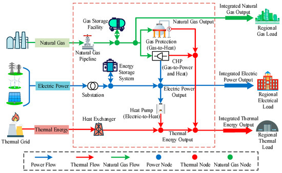
Figure 1.
Illustrates the energy transmission relationships in an integrated energy system.
Data from integrated energy systems exhibit both strong temporal dynamics and significant spatial correlations. Therefore, in analyzing load variation patterns, both periodic characteristics and inter-energy coupling properties are of paramount importance. Utilizing the correlations among various loads leads to improved accuracy in integrated energy load forecasting.
3. Analysis of Integrated Energy System Coupling Characteristics
In an integrated energy system, thermal and gas loads exhibit inertia in comparison to electrical loads, meaning they experience delayed fluctuations. In other words, the fluctuations in thermal and gas loads are influenced by the fluctuation patterns of electrical loads, and the correlation of the entire sequence evolves over time. Additionally, the vibration of thermal and gas loads is stable, and they do not experience drastic load fluctuations in the short term. DTW accounts for the delayed oscillation patterns in load data. Offline training is employed to preserve the coupling characteristics of the sequence as much as possible.
DTW works by identifying corresponding points of fluctuation between time series and calculating a relative distance to measure their correlation, enabling better handling of time-shifted relationships in time series data. In most cases, the oscillations of integrated energy loads appear very similar as a whole, but their initial starting points occur at different times, exhibiting a certain degree of delay. Therefore, before calculating the correlation between two time series, one or more of the time series are distorted or adjusted, either compressed or stretched, along the time axis in order to compute the correlation of the time series.
Given two time series, and , to compute their distance, we first need to generate an matrix, denoted as , where each element represents the Euclidean distance between and , as specified in Equation (1).
DTW finds the shortest distance path from one sequence to another in the distance matrix . This step can be solved using dynamic programming (DP), summing up the shortest path from the top-left corner of the matrix to the bottom-right corner. Assuming the matrix is , and the shortest path from the top-left corner to any coordinate point is , the optimal path can be obtained through recursive Equation (2).
Employing DTW on multi-energy data to investigate system coupling, the optimal dynamic warping paths were derived and are visualized in Figure 2. The shortest distances d between electricity, heat, and gas are, respectively, illustrated in Table 1. From Figure 2, it can be observed that both heat and gas loads exhibit significant delays compared to electricity loads, with heat loads being delayed relative to gas loads. The relatively low DTW distances between electricity-heat and heat-gas loads, presented in Table 1, indicate a strong coupling relationship after temporal warping.
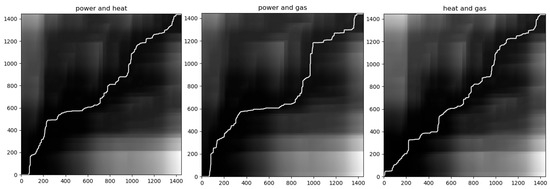
Figure 2.
Dynamic programming paths for multi-energy DTW.

Table 1.
Multi-energy DTW distances.
4. Two-Dimensional Feature Extraction Network
4.1. Multi-View Coupling Feature Extraction Model
Accounting for the nonlinear characteristics of multi-energy coupling, temporal data coupling analysis is performed using sliding convolutional windows. In practical multi-energy systems, coupling effects inherently exhibit temporal delays, the duration of which varies significantly across different operational contexts, time periods, and energy types. A key limitation of the single-layer sliding window approach is its fixed-size receptive field, which is inadequate for capturing the complex coupling characteristics of multi-energy systems. Under a fixed kernel size, the receptive field (RF) can be continuously expanded by adding more convolutional layers. The coupling feature extraction model is illustrated in Figure 3.
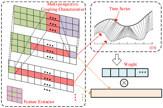
Figure 3.
Coupling Feature Extractor.
The different field coupling features mapped by multiple layers of sliding convolutional windows can be analyzed using the following formula:
where represents the field of view of the nth layer coupling feature; denotes the convolution kernel size of the n − 1 layer; represents the sliding window stride of the nth layer. In the multi-field coupling feature extraction model proposed in this paper, the convolution kernel and stride are set to fixed values of 3 × 3 and 1, respectively.
After multiple iterations of sliding windows, the result of the nth layer iteration is as follows:
To reasonably allocate the weights of coupling features under different fields of view, the associated distance of the layer iteration result is calculated through DTW, followed by activation function. The specific formula is as follows:
where . represents the weight vector of coupling features; denotes the result of the layer iteration; represents the coupling feature vector.
4.2. Two-Dimensional Temporal-Coupling Feature Extraction Model
Data used for load forecasting incorporates both coupled relationships across variables and critical temporal information. The two-dimensional feature extraction network (TDN) nonlinearly fuses temporal features and coupling features through multiple gating units. This gate-mediated recombination enables the simultaneous selection of spatiotemporal characteristics and historical patterns. The specific structural diagram principle is shown in Figure 4.
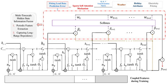
Figure 4.
Two-dimensional feature extraction network.
The integration of two-dimensional input features is achieved through the actions of two gating units, with the specific calculation formula as follows:
where represents the sigmoid activation function; b denotes the network bias; and respectively represent the coupling features and temporal features; signifies the network weight; tanh is the activation function; denotes the element-wise Hadamard product.
In temporal feature extraction models, information transmission is constrained by distance, leading to feature loss throughout the training and learning process. To store long-distance dependency information, multiple time-scale hidden state fusion is adopted to enhance the extraction of long-distance features for downstream tasks.
The feature deletion and memory of the TDN are achieved using backpropagation neural networks, which possess memory, retention, forgetting, and fusion capabilities, making them more suitable for handling temporally related tasks, particularly those associated with periodicity. Its forward propagation mechanism is analogous to that of LSTM networks, leveraging both memory cells and hidden states to preserve historical sequence information. The memory cells, controlled by three gating units, store the historical information of the sequence data. The formula is as follows:
The equation comprises: as the candidate memory unit used for updating the memory unit; represents the hidden state information; and stands for the output prediction result.
To address the issue of loss of periodic information due to long-distance data transmission, a feature periodic correlation vector is constructed, as shown in the formula below:
where denotes the hidden state information matrix; signifies the weight parameter of the hidden state feature; represents the weight matrix; and denotes the model’s output result.
The principles of two-dimensional temporal feature extraction retain the network’s memory function, where each time step’s hidden state possesses all previous time step features and oscillation patterns. The correlation of load at different positions within the sequence is enhanced, corresponding to an increase in the correlation of hidden state information within the respective period. Therefore, through the fusion of information across multiple time scales, it is relatively easy to compute periodic features, thereby better addressing the long-distance dependency issue in temporal networks and resolving the network’s dependence on the last time information. Obtaining global information enables the model to efficiently integrate multidimensional features.
Embedding encoding is employed to transform categorical features, such as weather, holidays, and electricity prices, into a spatial mapping, thereby enhancing the representation of inter-feature correlations. Model employs a sparse self-attention mechanism that amalgamates the expansion and Topk approaches. This integration allows for the simultaneous capture of global and salient information while effectively alleviating the computational burden associated with the self-attention’s spatial complexity.
4.3. Adaptive Learning Algorithm
In recent years, amidst the continuous evolution of neural networks, there has been a growing focus on adjusting network structures to achieve greater reductions in loss functions; Enhancing optimization algorithms to accelerate the rate of reduction in model loss functions; And handling input data to mitigate the impact of dimensionalities on network training. While existing methods enhance model accuracy and convergence rates, they lack mechanisms for dynamic network architecture adaptation.
AP effectively mitigates these limitations. At its core, AP employs a neural self-growth mechanism that enables dynamic adaptation of network size based on training data volume. The implementation of AP algorithms improves both the transferability and structural adaptability of network models. The structural principles of AP algorithms are depicted in Figure 5.
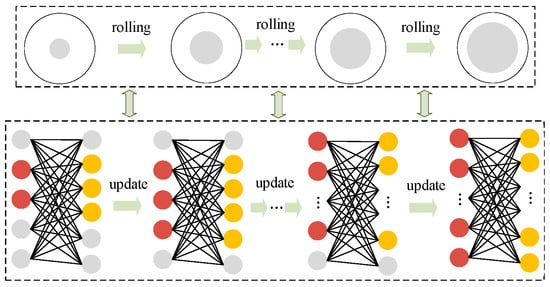
Figure 5.
Adaptive algorithm structure. In this diagram, red and yellow represent two distinct layers of neurons, while gray denotes neurons that are not activated.
The essence of the adaptive algorithm lies in activating certain neurons through a mechanism when the training data volume reaches a certain upper limit, enabling their participation in subsequent network training. In summary, the formula for the network structure employing the adaptive algorithm is as follows:
where denotes the number of neurons in layer; represents the threshold of data volume for adding neurons, i.e., every layer adds 16 neurons when the additional training data volume reaches p; and respectively represent the minimum and maximum network structures; represents the real-time incoming training data volume, is the maximum data volume that the minimum network structure can be trained on, and represents the maximum data volume that the network can handle. In this paper, based on existing research [19,20], p is set to 600, is set to 16, and is set to 600, while is determined by the maximum neuron structure of the network.
where represents the weight of layer , is the weight of layer after the adaptive algorithm, represents the output of layer , is the bias of layer , is the output of layer before the activation function , is an m-dimensional column vector with all elements being 1, and represents the Kronecker product.
The pseudocode for AP-CFE is shown in Algorithm 1. To achieve full-view observation for convolutions, compute the number of convolutional layers L. Across all training datasets, the AP algorithm and matrix multiplication are utilized to perform forward propagation. The backpropagation algorithm is then applied to minimize the error, leading to iterative updates of all convolutional kernel parameters. Embedding encoding maps the features of external factors (weather, holidays, electricity prices) into dense vector representations, which effectively captures the implicit relationships between them. Sparse self-attention mechanisms enable dense operations without compromising performance, significantly reducing runtime and minimizing memory usage. The training process was terminated after 100 epochs when the model’s validation error stabilized, indicating convergence.
| Algorithm 1: AP-CFE Algorithm |
 |
5. Case Analysis
5.1. Data Preprocessing
In a Python 3.11.8 simulation environment, the network architecture was constructed using TensorFlow 2.8. The experiment is conducted within the context of Denmark and New South Wales, Australia. Data samples are sourced from the Australian Energy Market Operator (https://www.aemo.com.au/) and the Australian Bureau of Statistics(https://www.energy.gov.au/). Due to the varying coupling relationships among different energy sources, a singular linear relationship cannot be employed for qualitative and quantitative analysis. Therefore, a multi-feature extraction approach is utilized to incorporate nonlinear computations, thereby delineating multidimensional characteristics among energy sources. The study employs load data from 1 August 2020, to 1 September 2020, with a sampling interval of 30 min (yielding 1536 data points). Input data comprise historical load data from the preceding 10 h. The data is partitioned into training, validation, and test sets in a ratio of 6:3:1, respectively. Preprocess data using maximum-minimum normalization [21]. The data preprocessing process is outlined as follows:
where z represents the maximum sample data within each dataset, denotes the minimum sample data, and signifies the normalized value.
5.2. Evaluation Metrics
The predictive performance of the load forecasting model is influenced by both predictive accuracy and prediction time. This study adopts the Mean Absolute Percentage Error (MAPE), Root Mean Square Error (RMSE) and Standard deviation (S) as evaluation metrics for the model’s predictive accuracy. The definitions of MAPE, RMSE and S are as follows:
where represents the number of predicted samples, and respectively denote the true value and the predicted value of the th sample, represents prediction error, represents the average prediction error and Accuracy denotes the model’s accuracy.
5.3. Evaluation Metrics Optimization Analysis of LSTM, CNN, TDN, and AP-CFE
To validate the contributions of coupled feature extraction, AP algorithms, and periodic feature extraction, we compare the LSTM, CNN, TDN, and the proposed AP-CFE model. The comparison results of the four models are shown in Figure 6.
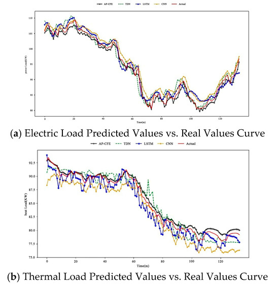
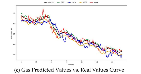
Figure 6.
Electric, Thermal, and Gas Load Prediction Curves.
Overall, in Figure 6, the electric load fluctuates most significantly in the multi-energy system, while the thermal load exhibits the most stable changes. The coupled features in the multi-energy system lead to delays in the thermal and gas loads compared to the electric load. Short-term downward trends in the electric load affect the changes in the thermal and gas loads. Among them, in the multi-energy system, the short-term variation range of the thermal load is the smallest, and the electric load is significantly affected by various factors, showing pronounced oscillations.
From Figure 6a, it can be observed that during the decline of the electric load, there is a significant decrease in load at the 20th sampling point, followed by a trend of oscillation and then an increase in load. In the 134 sampling points of the testing dataset, the span of the electric load’s extremes is 30 MW. Figure 6b shows the variation in the thermal load, which remains relatively stable overall. Only at the 55th sampling point, there is a downward trend in load, which lags behind the electric load. The fluctuation pattern of the electric load affects the oscillation of the thermal load, making it the slowest-changing load among the multi-energy loads. The energy conversion and transmission of electric and thermal loads are implemented by CHP (Combined Heat and Power), while heating equipment such as air conditioning is electrically driven, increasing the correlation between electric and thermal loads. The predicted results of the gas load are shown in Figure 6c, with the overall fluctuation ranging from 75 MW to 96 MW, and the inflection point of load decline occurring at the 35th sampling point, between the electric and thermal loads.
Among the four prediction models, the CNN model exhibits the most pronounced lag phenomenon, with the lowest accuracy, largest mean error, and dispersed distribution. The TDN model greatly improves the decrease in prediction accuracy caused by LSTM’s inability to extract coupled and periodic features. However, the inclusion of the CNN model leads to more complex backpropagation computations in the TDN model, requiring longer model training times.
The high coupling and periodicity of electricity loads result in a significant decrease in errors when employing the ensemble TDN. The relatively stable fluctuation patterns of heat and gas loads can reduce the complexity of model learning, with the LSTM model performing best in fitting the low-coupling gas load. From Figure 6 and Table 2, it can be observed that all four models can reasonably predict the approximate variation curves of the three loads. However, the proposed model (AP-CFE) can better describe the load fluctuation and anomaly features, with a more concentrated error distribution and relatively smaller MAPE and RMSE.
Table 2.
Evaluation Metrics of Four Prediction Models.
The AP-CFE enhanced by an adaptive learning algorithm with neuron self-growth mechanisms, enables optimization training that better conforms to the structural features of the data, while saving more time for training. Compared to the LSTM model, the proposed AP-CFE model reduces MAPE values by 34.03%, 34.68%, and 36.36%.
Table 3 shows the computational efficiency of the models. Given the same amount of data, LSTM typically train the fastest and consume the least memory; CNN train the slowest and consume the most memory; TDN and AP-CFE fall between the two.
Table 3.
Computational Efficiency of Four Models.
5.4. Model Comparison
To validate the superiority of the proposed method in terms of prediction accuracy and speed, the AP-CFE method is compared with methods from reference [18] (Bi-LSTM), ref. [16] (PatchTST), ref. [15] (FEDFormer), ref. [17] (CNN-GRU), and ref. [14] (EMD). The parameter settings for the five comparison prediction models are listed in Table 4.
Table 4.
Parameter Settings of Comparative Models.
Figure 7 illustrates the prediction curves of electricity, heat, and gas loads for each model. To evaluate the prediction accuracy of the models, the percentage error is used to analyze the error distribution of load prediction models, as shown in Figure 7.
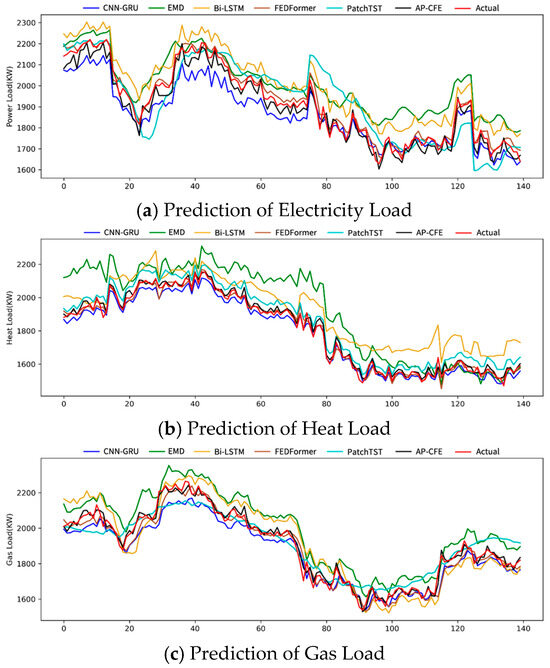
Figure 7.
Comparative curves of multi-energy Loads Forecasting in Australia.
From Figure 7 and Table 5, it can be observed that the FEDFormer model has a good fitting effect; the Bi-LSTM has the worst fitting effect because the fully connected layer cannot extract temporal or spatial features effectively; the EMD model decomposes and reconstructs the input data, ignoring the changing patterns of anomalies and outliers, which leads to inaccurate predictions for certain special values; the prediction effect of the CNN-GRU model deteriorates in the gas load, mainly due to the decreased coupling of gas load compared to electricity load.
Table 5.
Evaluation Metrics of Prediction Models in Australia.
Additionally, the energy conversion between electricity, heat, and gas greatly increases the difficulty of feature extraction for electricity load, resulting in lower overall prediction accuracy for electricity load. The error of the comparison model differs significantly from that of AP-CFE, indicating that the predictive accuracy of the comparison model needs improvement.
To evaluate the model’s generalization capability, additional simulation comparison experiments were conducted in the Danish region. The results are shown in Figure 8 and Table 6. The p-value of less than 0.05 indicates that the error of the AP-CFE model differs significantly from that of other models. The AP-CFE model also demonstrated the best predictive performance in the Danish region. The predictive performance of Bi-LSTM outperforms that of EMD, which differs from the forecast results in New South Wales, Australia. Meanwhile, PatchTST’s predictive performance is the closest to AP-CFE.
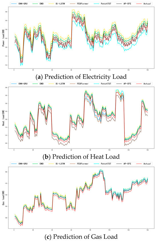
Figure 8.
Comparative curves of multi-energy Loads Forecasting in Denmark.
Table 6.
Evaluation Metrics of Prediction Models in Denmark.
6. Conclusions
This study integrates a multi-modal feature extraction framework with an AP algorithm for comprehensive energy load forecasting. The proposed approach aims to enhance the prediction accuracy of electricity, heat, and gas loads while improving model adaptability and computational efficiency.
The TDN architecture enhances the network’s capacity for nonlinear modeling, enabling the effective extraction of high-dimensional temporal, periodic, and coupling features from load data. Training three sets of networks with identical structures but different weights and biases enables the model to meet the requirements of different load types. Each network extracts both temporal variations and spatial coupling features. Sparse self-attention effectively reduces the spatial computational complexity of self-attention.
Compared to existing load forecasting models, the proposed AP-CFE model more effectively captures the dynamic patterns of integrated energy loads and provides enhanced characterization of multi-energy temporal dynamics and coupling relationships. This enables adaptive updates of the network structure, reducing both training and prediction times, and enhancing the model’s stability, accuracy, and adaptability. Load is influenced by multiple factors including weather, holidays, market electricity prices, and renewable energy output. Future model architectures must adopt a unified framework capable of naturally processing multimodal inputs while simultaneously accomplishing multiple related tasks.
Author Contributions
Y.Q. conceived the idea for the manuscript, B.H. (Bonan Huang), Y.Z. (Yameng Zhang), L.W. (Luyuan Wang) and J.T. (Jiaqi Tian) wrote the manuscript. All authors have read and agreed to the published version of the manuscript.
Funding
This work was supported in part by the National Natural Science Foundation of China under Grant 52377079.
Data Availability Statement
Data downloads are available at links (https://www.aemo.com.au/) and (https://www.energy.gov.au/). Data processing are contained within the article.
Conflicts of Interest
The authors declare no conflict of interest.
References
- Wang, L.; Song, H.; Yu, Q. The Application of Hybrid Deep Learning Method of Improved Transformer Model in Load Forecasting Based on Future Network and Edge Computing. Int. J. High Speed Electron. Syst. 2025, 2540848. [Google Scholar] [CrossRef]
- Xu, B.; Zhang, Y. Development Path of Regional Integrated Energy System; IOP Publishing: Bristol, UK, 2019. [Google Scholar]
- Liu, L.; Wang, D.; Hou, K. Region model and application of regional integrated energy system security analysis. Appl. Energy 2025, 260, 114268. [Google Scholar] [CrossRef]
- Liu, X.; Wu, K.; Qi, L. Multi-Objective Optimization Design of Regional Integrated Energy System; IOP Publishing: Bristol, UK, 2020. [Google Scholar]
- Lorenzo, B.; Stefano, C.; Vincenzo, M. Short-term forecasting method to improve the performance of a model predictive control strategy for a residential hybrid renewable energy system. Energy 2019, 172, 997–1004. [Google Scholar]
- Andersen, F.; Larsen, H.; Gaardestrup, R. Long term forecasting of hourly electricity consumption in local areas in Denmark. Appl. Energy 2013, 110, 147–162. [Google Scholar] [CrossRef]
- Duan, Q.; Liu, J.; Zhao, D. Short term electric load forecasting using an automated system of model choice. Int. J. Electr. Power Energy Syst. 2017, 91, 92–100. [Google Scholar] [CrossRef]
- Moazzami, M.; Khodabakhshlan, A.; Hooshmand, R. A new hybrid day-ahead peak load forecasting method for Iran’s National Grid. Appl. Energy 2013, 101, 489–501. [Google Scholar] [CrossRef]
- Maryam, I.; Hassan, G. Residential load forecasting using wavelet and collaborative representation transforms. Appl. Energy 2019, 253, 113505. [Google Scholar] [CrossRef]
- Mohan, N.; Soman, K.; Kumar, S. A data-driven strategy for short-term electric load forecasting using dynamic mode decomposition model. Appl. Energy 2018, 232, 229–244. [Google Scholar] [CrossRef]
- Yang, D.; Guo, J.; Sun, S. An interval decomposition-ensemble approach with data-characteristic-driven reconstruction for short-term load forecasting. Appl. Energy 2022, 306, 117992. [Google Scholar] [CrossRef]
- Yu, F.; Xu, X. A short-term load forecasting model of natural gas based on optimized genetic algorithm and improved BP neural network. Appl. Energy 2014, 134, 102–113. [Google Scholar] [CrossRef]
- Yin, L.; Xie, I. Multi-temporal-spatial-scale temporal convolution network for short-term load forecasting of power systems. Appl. Energy 2021, 283, 116328. [Google Scholar] [CrossRef]
- Wang, X.; Wang, S.; Zhao, Q. A multi-energy load prediction model based on deep multi-task learning and ensemble approach for regional integrated energy systems. Int. J. Electr. Power Energy Syst. 2021, 126, 106583. [Google Scholar]
- Jin, X.; Pan, T.; Yu, H. Electricity Load Forecasting Method Based on the GRA-FEDformer Algorithm. Energies 2025, 18, 4057. [Google Scholar] [CrossRef]
- Gong, M.; Yang, Y.; Huang, J.; Cui, H.; Jing, S.; Zhang, F. A novel wind power prediction model based on PatchTST and temporal convolutional network. Environ. Prog. Sustain. Energy 2025, 44, e14584. [Google Scholar] [CrossRef]
- Yuan, Q.; Li, H.; Pan, Y. Research on Hybrid Model for Short-term Power Load Forecasting Based on Error Compensation. IAENG Int. J. Comput. Sci. 2025, 52, 2719–2725. [Google Scholar]
- Wen, C.; Guang, H.; Hong, Z.; Lyuchao, L. Short-Term Load Forecasting with an Ensemble Model Using Densely Residual Block and Bi-LSTM Based on the Attention Mechanism. Sustainability 2022, 14, 16433. [Google Scholar]
- Zhong, C.; Liu, S.; Lu, Q.; Zhang, B.; Wang, J.; Xu, Q. Topological structural analysis based on self-adaptive growing neural network for shape feature extraction. Neurocomputing 2022, 503, 219–235. [Google Scholar] [CrossRef]
- Mazurov, M.; Mikryukov, A.; Gorbatih, M.; Bergaliev, T.; Shchukina, N. Information and neural educational system for training standard and selective neural network technologies in universities. CEUR Workshop Proc. 2021, 2919, 161–173. [Google Scholar]
- Viet, D.; Phuong, V.; Duong, M.; Tran, Q. Models for Short-Term Wind Power Forecasting Based on Improved Artificial Neural Network Using Particle Swarm Optimization and Genetic Algorithms. Energies 2020, 13, 2873. [Google Scholar] [CrossRef]


Disclaimer/Publisher’s Note: The statements, opinions and data contained in all publications are solely those of the individual author(s) and contributor(s) and not of MDPI and/or the editor(s). MDPI and/or the editor(s) disclaim responsibility for any injury to people or property resulting from any ideas, methods, instructions or products referred to in the content. |
© 2025 by the authors. Licensee MDPI, Basel, Switzerland. This article is an open access article distributed under the terms and conditions of the Creative Commons Attribution (CC BY) license (https://creativecommons.org/licenses/by/4.0/).