Article

Balanced Neonatal Cry Classification: Integrating Preterm and Full-Term Data for RDS Screening

by
Somaye Valizade Shayegh
* and
Chakib Tadj
Department of Electrical Engineering, École de Technologie Supérieure, Université du Québec, Montréal, QC H3C 1K3, Canada
*
Author to whom correspondence should be addressed.
Information 2025, 16(11), 1008; https://doi.org/10.3390/info16111008
Submission received: 23 September 2025 / Revised: 18 October 2025 / Accepted: 11 November 2025 / Published: 19 November 2025
(This article belongs to the Special Issue Biomedical Signal and Image Processing with Artificial Intelligence)

Abstract

Respiratory distress syndrome (RDS) is one of the most serious neonatal conditions, frequently leading to respiratory failure and death in low-resource settings. Early detection is therefore critical, particularly where access to advanced diagnostic tools is limited. Recent advances in machine learning have enabled non-invasive neonatal cry diagnostic systems (NCDSs) for early screening. To the best of our knowledge, this is the first cry-based RDS detection study to include both preterm and full-term infants in a subject-balanced design, using 76 neonates (38 RDS, 38 healthy; 19 per subgroup) and 8534 expiratory cry segments (4267 per class). Cry waveforms were converted to mono, high-pass-filtered, and segmented to isolate expiratory units. Mel-Frequency Cepstral Coefficients (MFCCs) and Filterbank (FBANK) features were extracted and transformed into fixed-dimensional embeddings using a lightweight X-vector model with mean-SDor attention-based pooling, followed by a binary classifier. Model parameters were optimized via grid search. Performance was evaluated using accuracy, precision, recall, F1-score, and ROC–AUC under stratified 10-fold cross-validation. MFCC + mean–SD achieved 93.59 ± 0.48% accuracy, while MFCC + attention reached 93.53 ± 0.52% accuracy with slightly higher precision, reducing false RDS alarms and improving clinical reliability. To enhance interpretability, Integrated Gradients were applied to MFCC and FBANK features to reveal the spectral regions contributing most to the decision. Overall, the proposed NCDS reliably distinguishes RDS from healthy cries and generalizes across neonatal subgroups despite the greater variability in preterm vocalizations.

1. Introduction

In 2023, the global under-five mortality rate stood at 37 per 1000 live births, with neonatal mortality (within the first 28 days) contributing 17 per 1000—equating to approximately 2.3 million deaths annually, or 6300 per day [1,2]. These figures, reaffirmed by the World Health Organization in mid-2024, highlight the persistent challenge of neonatal survival, particularly in low-resource settings [3]. A global scoping review by Tochie et al. [4] identified RDS as the leading cause of neonatal respiratory failure, with reported hospital-based mortality ranging from 0.2% to 57.3% in under-resourced regions such as Ethiopia. Supporting this, a retrospective study of Ethiopian public hospitals (2019–2021) reported a 37.4% mortality rate among neonates with RDS, corresponding to 59.9 deaths per 1000 neonatal-days [5].
Since the 1960s, the analysis of newborn cries for diagnostic purposes has advanced significantly. Pioneering work by Wasz-Höckert et al. in Scandinavia used spectrographic analysis to distinguish typical cries from those associated with conditions such as Down’s syndrome [6], laying the groundwork for neonatal cry analysis. Modern NCDSs have evolved from basic acoustic assessments to data-driven models that extract clinically relevant biomarkers from cry signals. They offer a non-invasive, accessible means of early warning to aid clinical screening and intervention, particularly in low-resource settings.
This study aims to develop a practical and reliable NCDS for early detection of RDS. We utilize a private cry dataset balanced across RDS and healthy cases, including both preterm and full-term infants to improve generalizability. Table 1 details the characteristics of the selected CASs (Cry Audio Signals) for the current study. Pre-emphasis filtering and manual segmentation are applied to isolate diagnostically relevant expiratory cry segments. FBANKs and MFCCs are extracted as low-level features and input to a lightweight X-vector model, which encodes variable-length cries into fixed-dimensional embeddings via statistical or attention-based pooling. A classifier then maps these embeddings to RDS or healthy labels by capturing underlying acoustic patterns.
The remainder of this paper is organized as follows: Section 2 reviews related work to establish the theoretical and empirical context. Section 3 details the materials and methods, including the data pipeline, feature extraction, embedding and classification strategies, customized X-vector training, Interpretability Methods, hyperparameter tuning, and evaluation protocol. Section 4 presents results and analysis, highlighting the performance of MFCC and FBANK features with statistical and attention-based pooling. Finally, Section 5 discusses the findings and concludes this paper.

2. Literature Review

Machine learning (ML) models have shown strong potential in infant cry classification, with reported accuracies exceeding 80%—a significant improvement over the average human performance of 34% [7]. This gap highlights the ability of computational models to detect subtle, clinically relevant acoustic patterns often imperceptible to human listeners, reinforcing their value as non-invasive tools for automated health screening. The field of cry analysis has advanced substantially, as evidenced by a systematic review of 126 studies conducted over a 24-year period [8]. Early efforts relied on statistical models and manually defined decision rules using limited acoustic features. More recently, the field has shifted toward data-driven methods, with ML, deep learning (DL), and hybrid architectures forming the core of modern systems. This transition reflects both technological advances and growing recognition of infant cries as valuable biomarkers for neonatal health. Ji et al. [9] illustrate the application of these methods across tasks such as cry reason classification, cry detection, and pathological cry identification. Among these, identifying pathological cries remains the most challenging due to significant acoustic variability and limited clinical data. Data scarcity—driven by ethical concerns, the vulnerability of neonates, and difficulties in obtaining parental consent—continues to hinder scalability and clinical adoption of cry-based diagnostic tools.
Although research in automatic infant cry analysis is growing, few studies have specifically focused on classifying RDS. Our group has explored this challenge using various feature representations, classification models, and population cohorts. The first study [10] framed the task as binary classification. It employed MFCCs, tilt, and rhythm features to capture both short-term spectral cues and long-term dynamics, achieving 73.8% accuracy using a linear Support Vector Machine (SVM) on expiratory segments. Subsequent works extended the task to three-class classification, typically distinguishing healthy, RDS, and sepsis cries. The third study  [11] employed a fusion-based approach using spectrograms of expiratory (EXP) cries as input to a CNN pretrained on ImageNet for deep feature extraction. The resulting embeddings were combined with prosodic and spectral features—HR and GFCCs— used to train various classifiers, including Random Forest (RF), SVM, and Deep Neural Networks (DNNs); the DNN achieved the highest accuracy of 97.5%. The fourth study [12] used the dataset from [11] to classify healthy, RDS, and sepsis cries by converting expiratory (EXP) segments into spectrogram images. A Vision Transformer (ViT) was applied to capture the most informative spectral regions via self-attention, achieving 98.69% accuracy. The fifth study [13] also used image-based audio inputs—GFCCs, spectrograms, and mel-spectrograms—as input to a Vision Transformer (ViT), with GFCCs yielding the highest accuracy (96.33%). To improve interpretability, the authors applied explainable AI techniques, including Layer-wise Relevance Propagation (LRP), LIME, and attention visualization. In the final study [14], self-supervised models—wav2vec, WavLM, and HuBERT—were fine-tuned on a balanced EXP dataset to extract features directly from raw cry signals, and then a single fully connected layer was used for classification, with wav2vec achieving the highest accuracy (89.76%) and annealing learning rate schedules outperforming linear ones. The study emphasizes the benefits of raw audio input in streamlining the processing pipeline and advancing NCDSs. Although all studies from the group used the same private database and focused solely on full-term newborns, they differed in cry sample counts and segment durations. Studies 1–5 maintained class-balanced samples but showed uneven infant distribution across classes, raising concerns about subject-level bias. In contrast, ref. [14] utilized a larger dataset with equal infant representation across RDS, healthy, and sepsis classes, improving the robustness and generalizability of the results.
MFCCs remain a cornerstone feature in NCDSs, consistently used as direct inputs or within pre-processing pipelines for deep learning models. Their enduring use—despite growing model complexity—reflects their effectiveness in capturing key spectral and perceptual properties of infant cries [8,9], supporting their integration across both traditional and end-to-end architectures. In contrast, Filterbank energies (FBANKs) retain spectral detail by omitting the cepstral transformation, yet remain underutilized in NCDSs. Their raw spectral fidelity makes them well-suited for deep learning models that learn hierarchical representations. FBANK features have shown strong performance in related domains—speech recognition [15], respiratory sound classification [16], and environmental audio analysis [17]—thereby underscoring their untapped potential for infant cry analysis and warranting further investigation. MFCCs have been widely used to distinguish healthy from unhealty infant cries. In [18], MFCCs were combined with auditory-inspired amplitude modulation (AAM) features and classified using an SVM on expiratory segments. Similarly, ref. [19] extracted MFCCs and GFCCs, enhanced them via Canonical Correlation Discriminant Features (CCDFs), and used an LSTM network for classification. Complementary to these studies, ref. [20] compared MFCCs with Constant Q Cepstral Coefficients (CQCCs), Linear Frequency Cepstral Coefficients (LFCCs), and Short-Time Fourier Transform (STFT)-based features on the Baby Chillanto dataset, reporting superior performance with CQCCs using Gaussian Mixture Model (GMM) classifiers. In [21], MFCCs were extracted from the iCOPE dataset along with additional spectral and spectrogram-based descriptors (e.g., Local Binary Patterns (LBPs), Local Phase Quantization (LPQ), and Rotation-Invariant LBP (RLBP)). Classification was improved using SVMs and feature fusion techniques. Similarly, ref. [22] used GMM-UBM models trained on static and dynamic MFCCs from both expiratory and inspiratory segments to distinguish pathological from healthy cries.
In [23], the classification of healthy versus septic newborns was explored. MFCCs were extracted alongside prosodic features—intensity, rhythm, and tilt—from both expiratory and inspiratory segments. Each feature set was evaluated individually and in combination using various classifiers and majority voting. For expiratory cries, the highest F-score was achieved by an SVM trained on the full feature set, while for inspiratory segments, tilt features combined with a quadratic discriminant classifier performed best. Several studies have addressed the classification of asphyxiated versus healthy newborn cries using acoustic and prosodic features. In [24], MFCCs were extracted from cry recordings and fed into a CNN for binary classification. Similarly, ref. [25] used a combination of acoustic features—MFCCs, chromograms, spectral contrast, and tonnetz—to train deep learning models. CNNs performed best with MFCCs alone, while DNNs achieved higher accuracy using the full feature set. In [26], Weighted Prosodic Features—including pitch, energy, intensity, F0, and formants—were used to train a DNN for classifying cries as healthy or asphyxiated. The study also proposed a hybrid approach, combining MFCCs and prosodic features into a joint matrix fed into a second DNN, further improving classification performance.
In [27], infant cries were analyzed to distinguish healthy infants from those with Autism Spectrum Disorder (ASD). Four acoustic feature types—MFCCs, LPCCs, wavelet coefficients, and DWT-MFCCs—were used to train SVM and CNN classifiers. DWT-MFCCs yielded the highest accuracy and noise robustness with SVM, while MFCCs performed best with CNNs. The findings suggest that MFCCs are well-suited for deep learning, while wavelet-based features enhance robustness for real-world ASD cry detection. In [28], the authors classified healthy versus Hypoxic–Ischemic Encephalopathy (HIE) cries using a privately curated dataset with manually segmented recordings to exclude inhalations and reduce noise. A range of spectral and cepstral features—including MFCCs, dynamic MFCCs, Gammatone Cepstral Coefficients, Spectral Centroid, entropy, and Flux—were extracted, followed by sequential feature selection. Classification was performed using a deep model with a BiLSTM layer, a fully connected layer, and a softmax output, demonstrating the feasibility of audio-based HIE detection. Multi-class cry classification has also been explored to differentiate among multiple pathologies. In [29], 16-dimensional MFCCs were extracted from 50 ms frames of a self-recorded dataset, reduced using PCA, and classified with an Adaptive Neuro-Fuzzy Inference System (ANFIS), which modeled fuzzy rules to distinguish deafness, asphyxia, and normal conditions. Similarly, ref. [30] proposed a more elaborate pipeline using the Baby Chillanto and Malaysian infant cry datasets. Each sample was represented by 568 features, including 496 wavelet packet transform-based entropy measures (e.g., Tsallis, Renyi, Shannon, permutation, fuzzy, approximate, and sample entropy), 56 LPCCs, and 16 MFCCs. Dimensionality was reduced using the Improved Binary Dragonfly Optimization (IBDFO) algorithm, selecting the top 204 features to train an Extreme Learning Machine (ELM) kernel classifier.
The X-vector architecture, introduced by Snyder et al. [31], was originally designed for speaker recognition, transforming variable-length audio into fixed-dimensional embeddings using Time-Delay Neural Network (TDNN) layers followed by statistical pooling. Its ability to capture both local and global acoustic patterns makes it adaptable to a wide range of speech and audio classification tasks. It has been successfully applied in multi-speaker recognition [32], spoken language identification [33], and robust speaker verification in noisy environments [34]. Its utility further extends to low-resource speech recognition [35], acoustic scene classification [36], and blind audio source separation guided by speaker identity [37]. Although not yet utilized in newborn cry analysis, the X-vector framework is well-suited for NCDSs due to its ability to produce compact, discriminative embeddings—particularly when optimized for lightweight deployment on small-scale clinical datasets, as demonstrated in this study.
Despite increasing interest in NCDSs, research specifically targeting RDS detection from infant cries remains limited. Within our group, one study addressed binary classification of RDS versus healthy infants [10], while others explored three-class classification involving RDS, sepsis, and healthy conditions [11,12,13,14]. However, all of these studies focused solely on full-term newborns, leaving the more vulnerable preterm population underrepresented. Moreover, most relied on datasets with imbalanced infant distribution across classes. Although [14] adopted a balanced design, it was also limited to full-term infants. These limitations—lack of subject-level balance and exclusion of preterm neonates—substantially constrain the generalizability and clinical applicability of existing cry-based diagnostic models. Moreover, unifying classification for preterm and full-term infants adds complexity due to marked developmental differences in vocal characteristics during the first two months of life. Preterm cries typically exhibit higher and more unstable fundamental frequencies, flatter melodic contours, shorter and more irregular cry bursts, and reduced loudness and harmonic structure compared to those of full-term infants [38]. These acoustic differences arise from physiological immaturities, including underdeveloped lungs, thinner vocal folds, and incomplete neuromuscular coordination [39]. Consequently, preterm cries are inherently noisier and less structured, posing challenges for developing classifiers that generalize across neonatal subgroups.
To address prior limitations, this study is the first to incorporate cry recordings from both preterm and full-term infants across RDS and healthy cases. A balanced cohort was formed by selecting 19 newborns of both sexes for each of the four clinical groups: RDS/preterm, RDS/full-term, healthy/preterm, and healthy/full-term. All recordings were collected with informed parental consent and in compliance with ethical guidelines. This subject-balanced, demographically diverse dataset forms the basis of a novel cry-based classification framework for neonatal healthcare. This study makes two key contributions to cry-based disease detection. First, it presents the first subject-balanced classification system for distinguishing RDS and healthy cries across both preterm and full-term infants, addressing the critical gap left by prior studies that excluded preterm populations. Second, it introduces an efficient and scalable diagnostic framework using low-dimensional cepstral and spectral features—MFCCs and FBANKs—combined with a customized lightweight X-vector architecture. Variable-length acoustic inputs are transformed into discriminative fixed-length embeddings that capture key vocal characteristics across developmental stages. The model is trained via an optimized pipeline that accounts for acoustic variability in pitch, rhythm, and harmonic structure, enabling robust classification and demonstrating strong potential for non-invasive, clinically viable RDS screening.

3. Materials and Methods

The methodology begins with raw cry waveforms, which undergo stereo-to-mono conversion, high-pass FIR filtering, and manual segmentation to isolate expiratory segments. From these, low-level acoustic features—either FBANKs or MFCCs—are extracted. A customized lightweight X-vector model then transforms the variable-length features into fixed-dimensional embeddings. These are passed to a classifier to predict the infant’s condition as either healthy or affected by RDS. Figure 1 provides an overview of the complete pipeline, from raw input to final prediction.

3.1. Data Pipeline

This section describes the collection of newborn cry audio signals (CASs), outlines the dataset characteristics, details the pre-processing procedures, and presents the participant information used in the experiments.

3.1.1. Data Characteristics

This study utilized the private cry audio dataset described in [14], collected in collaboration with Al-Raee and Al-Sahel hospitals (Lebanon) and Sainte-Justine Hospital (Montreal, QC, Canada). Ethical approval was obtained, and informed consent was secured from guardians prior to data collection. CASs were recorded in natural clinical environments—including maternity wards and NICUs—at a sampling rate of 44.1 kHz and 16-bit resolution, with microphones positioned 10–30 cm from the newborn’s mouth. To preserve ecological validity, ambient sounds such as staff conversations, alarms, and other infants’ cries were intentionally retained.
Health conditions were determined through postnatal screening, and each cry was labeled as healthy or pathological based on medical records. The dataset comprises CASs from 769 newborns, representing 96 distinct pathologies, with some infants contributing multiple recordings (up to 5), each lasting 1–4 min (mean: 90 s). Infant ages ranged from 1 to 208 days. Cries were elicited by common stimuli, including hunger, discomfort, diaper changes, blood tests, bathing, and delivery. Recorded metadata includes cry trigger, gestational age, birth weight, Apgar score, gender, hospital, pathology type, age at recording, and prematurity status (full-term or preterm). The dataset reflects broad demographic diversity across races, ethnicities, and genders, including half-Caucasian and half-Haitian, African, Arabic, Caucasian, Latino, Native Hawaiian, and Québécois backgrounds. This diversity is relevant, as prenatal exposure to prosodic features during the third trimester may influence CAS production [40].
Although the dataset remains the same as in our previous study [14], the present work targets distinct clinical categories within the data, offering a new perspective on model performance across specific conditions.

3.1.2. Data Implementation

CASs were classified into two groups—RDS and healthy—based on two criteria. First, only infants younger than 54 days were included, as cry frequency remains stable and voluntary control is not yet developed at this age [41,42]. Second, both full-term and preterm newborns were considered. After applying these criteria, the dataset comprised 782 recordings from 303 healthy full-term newborns, 94 from 36 healthy preterm newborns, 102 from 35 full-term newborns with RDS, and 43 from 19 preterm newborns with RDS. To ensure balanced representation, 19 newborns of both genders were selected from each of the four groups. Recordings from healthy full-term and preterm infants were merged into a single ’healthy’ category, and those from RDS cases into an ’RDS’ category.
The pre-processing procedure in this study followed the approach detailed in [14] and consisted of three primary stages: conversion of stereo-channel recordings to mono via averaging; pre-emphasis filtering using a first-order high-pass FIR filter defined by
P ( z ) = 1 0.97 z 1 ,
which introduces a zero near z = 1 to compensate for the spectral tilt introduced by the glottal source; and segmentation. Each CAS typically contains multiple expiratory and inspiratory phases, along with behavioral and background sounds. Using WaveSurfer, these segments were manually labeled and extracted. This study specifically focused on expiratory segments (EXPs) due to their higher informational value, treating each EXP as an independent cry sample for subsequent processing and analysis. Table 1 summarizes the selected CASs, participant details, number of EXP segments, and the range of segment durations.
To ensure balanced representation, the RDS group (4317 EXP samples) was randomly downsampled to 4267 samples, matching the number of available samples in the healthy group. Given the dataset’s limited size and variable signal durations, stratified k-fold cross-validation was adopted to provide a more robust and reliable evaluation [43]. By preserving class proportions within each fold and allowing all samples to contribute to both training and validation, this approach mitigates the risk of overfitting, performance bias, and variability in model behavior.

3.2. Feature Extraction

Feature extraction transforms raw audio into compact representations to address the challenges of high-dimensional data. For example, CASs sampled at 44.1 kHz yield 44,100 samples per second, leading to significant computational complexity. Although DNNs can learn hierarchical representations, direct waveform processing is resource-intensive and prone to issues such as vanishing or exploding gradients. Using signal-derived low-dimensional features reduces complexity, stabilizes training, and supports robust representation learning. In this study, we employed two feature types: spectral domain (FBANKs) and cepstral domain (MFCCs).

3.2.1. Filterbank Features (FBANKs)

Spectral features such as filterbank energies (FBANKs) capture the distribution of signal energy across frequency bands over time. To extract FBANKs, the raw waveform is converted to the time–frequency domain (Figure 2). The signal is segmented into short frames, windowed, and transformed via FFT to obtain the power spectrum. A mel-scale filterbank is then applied, summing the energy within each filter, and the logarithm of these values yields the final FBANK features, following standard procedures in the HTK Book [44]. The mel scale, central to FBANKs, stems from psychophysical studies of pitch perception, approximating how humans perceive frequency differences. The scale maps real frequency values (Hz) to a perceptual scale: it is approximately linear below 1 kHz and logarithmic at higher frequencies. The mel scale is mathematically defined as follows:
Mel ( f ) = 2595 × log 10 1 + f 700 ,
where f is the frequency in Hertz (Hz), Mel ( f ) is the perceived pitch in Mel units, log 10 denotes the logarithm to base 10, and 2595 and 700 are empirically determined constants based on psychoacoustic experiments.

3.2.2. Mel-Frequency Cepstral Coefficients (MFCCs)

Following the extraction of FBANK features, MFCCs, introduced by Davis and Mermelstein [45], are obtained by applying the Discrete Cosine Transform (DCT) to the logarithm of the mel-scale filter bank outputs, as shown in Figure 2. The DCT reduces redundancy and removes correlation among the FBANK coefficients, transforming the energy distribution into a compact set of features that summarize the spectral shape. Cepstral features such as MFCCs capture the overall shape of the spectral envelope rather than individual frequency components, modeling how the spectral energy varies over time.
Since both FBANKs and MFCCs are extracted from audio signals of variable length, the resulting features are represented as two-dimensional matrices, where one axis corresponds to time frames and the other to the number of feature coefficients—FBANK energies or MFCCs, respectively. All feature extraction parameters, including those determining the number of time frames (e.g., window size, frame overlap, and signal duration), were optimized through the procedure described in Section 3.6. Moreover, to improve training stability and reduce variability, global mean-variance normalization (MVN) was applied to the MFCC and FBANK features before feeding them into the X-vector model. Common in both classical and modern systems [31,44], this process standardizes each feature dimension over the training set:
x i , d = x i , d μ d σ d ,
where x i , d is the value at frame i, dimension d and μ d , σ d are the global mean and standard deviation, respectively.

3.3. Feature Embedding and Classification

Following the extraction of low-level acoustic features (MFCCs and FBANKs), a higher-level representation is required to capture temporal and discriminative patterns in CASs. To this end, we adopt and adapt the X-vector architecture [31] for NCDS, targeting the classification of healthy versus RDS cries. The following sections review the original X-vector framework and its temporal modeling core, the TDNN [46], together with our customized implementation, forming the basis of the proposed system.
The X-vector model extracts low-dimensional, fixed-length embeddings from variable-length speech signals. Originally developed for speaker recognition, it has proven robust to noise, channel mismatch, and speaking style variation. Its architecture consists of stacked TDNN layers, a statistical pooling layer, fully connected layers, and a backend classifier. TDNNs process sliding windows of input frames to generate intermediate embeddings. Through varying kernel sizes and dilation factors, they expand the temporal receptive field, enabling the capture of both short- and long-range dependencies such as phonemes, syllables, or pathological cry patterns. Unlike feedforward networks that process frames independently, TDNNs integrate context from past and future frames, making them effective for modeling temporal dependencies in sequential audio. In modern frameworks, they are implemented as one-dimensional convolutions along the time axis, whose hierarchical structure yields increasingly abstract temporal representations. This makes TDNNs a foundational component of many audio classification systems, including the X-vector framework used in this study. In the X-vector architecture, the final TDNN output is passed to a statistical pooling layer that computes the mean and standard deviation of each feature dimension, converting variable-length inputs into fixed-length representations. Positioned between temporal encoding and the fully connected layers, this pooling bridges frame-level processing with sequence-level classification. The pooled vector then passes through two fully connected layers, with the first (typically 512 neurons) providing the X-vector embedding before the final classification stage. X-vectors encapsulate class-relevant temporal patterns. In training, the second fully connected layer (≈1500 neurons) is followed by a softmax for supervised classification with cross-entropy loss; these layers are optimized jointly with the network but discarded at inference. After extraction, a probabilistic linear discriminant analysis (PLDA) backend is trained separately to score embeddings by similarity. In the original implementation, training uses MFCCs with data augmentation (noise, reverberation, and channel distortion) to enhance generalization.
In this study, we employ a lightweight X-vector variant to encode variable-length neonatal cry signals into fixed-length embeddings. Although the original model—developed for large-scale speaker recognition—performs well, its high parameter count and rigid design limit applicability to small, domain-specific datasets. To overcome this, we implement a streamlined version that preserves the core elements of temporal modeling with TDNN layers, pooling, and dense embedding projection. Unlike the fixed original design, our architecture allows key design parameters—including the number of TDNN blocks, embedding dimensionality, pooling strategy, and dilation settings—to be optimized through a dedicated hyperparameter search. We also replace the PLDA backend with a single fully connected layer and sigmoid activation, providing an efficient classifier tailored to the constraints of NCDSs. As part of this flexible architecture, we investigate the effect of temporal summarization by implementing and comparing two pooling strategies: conventional statistics pooling and a customized attention-based pooling. The former aggregates frame-level embeddings using the global mean and standard deviation, treating all frames equally. In contrast, the attention-based pooling mechanism assigns learnable weights to individual frames, allowing the model to emphasize informative temporal regions. Inspired by attention mechanisms initially introduced for sequence modeling tasks [47] and later adapted for speaker embedding in speech processing [48], we incorporate a learnable projection layer to compute frame-level importance scores. To enhance representational diversity, we evaluate single- and multi-head attention, treating the number of heads as a tunable hyperparameter. Sequence-length masking is applied to suppress padded frames, ensuring robust aggregation across variable-length inputs.

3.4. Training of the Customized X-Vector

Each cry signal is transformed into a two-dimensional feature matrix via MFCC or FBANK extraction with fixed frame size and hop length. The resulting matrix has variable length, where rows correspond to time frames and columns to cepstral or spectral features. For a batch of cry segments with different durations, this yields matrices { X i } i = 1 N , where X i R T i × F , T i is the number of frames in the i-th segment, and F the feature dimension. This representation preserves the sequential structure of the acoustic signal, enabling the model to exploit both temporal and spectral information. To reduce variability and improve convergence, features are globally normalized using the mean and variance computed over the training set.
The normalized matrices are then processed by a stack of TDNN blocks, which apply one-dimensional convolutions along the time axis. By employing different kernel sizes and dilation rates, the TDNN layers progressively expand the temporal receptive field, allowing the model to capture both short- and long-range dependencies. The final TDNN output retains the temporal dimension and is subsequently passed to a pooling layer for sequence summarization.
(1) Statistics pooling. Given hidden sequences H i R T i × F from the TDNN for utterance i, we obtain a fixed-length representation by concatenating the per-feature mean and standard deviation across time:
z i stat = μ ( H i ) , σ ( H i ) R 2 F ,
Here, μ ( H i ) and σ ( H i ) are computed along the temporal axis, T i is the number of frames after the TDNN, F is the number of TDNN channels, and [ · , · ] denotes concatenation along the feature dimension.
(2) Attention-based pooling. To assign data-driven weights to frames—allowing the model to emphasize acoustically informative regions rather than treating all frames equally—we apply multi-head self-attention (MHA) to the TDNN representations. For each head, query, key, and value projections are
Q = H W Q , K = H W K , V = H W V ,
and scaled dot-product attention with key-padding mask M is
A = softmax Q K d k + M , Z = A V ,
Outputs from all heads are concatenated and projected:
MHA ( H ) = Concat ( Z 1 , , Z h ) W O ,
We then aggregate over time to obtain a fixed-length, context-weighted embedding:
z i mha = 1 T i t = 1 T i MHA ( H i ) [ t ] ,
z i mha = t = 1 T i m i , t MHA ( H i ) [ t ] t = 1 T i m i , t ( masked mean over valid frames ) ,
Here, H R T × F are hidden states (optionally projected to dimension F ); W Q , W K , W V R F × d k are learned projections; d k is the head dimension; A R T × T contains attention weights; Z R T × d k are per-head outputs; h is the number of heads; W O R ( h d k ) × F is the output projection; MHA ( H ) [ t ] R F is the t-th attended frame; and m i , t { 0 , 1 } masks padded frames for utterance i.
We train the TDNN–pooling encoder and linear classifier jointly end-to-end from random initialization using a single optimizer. Adam is employed with a linear learning-rate schedule that decays from the initial to the final rate across epochs. The classifier outputs a single logit, which is passed through a sigmoid and binarized at 0.5 for reporting. Training is guided by the binary cross-entropy (BCE) loss:
L BCE = 1 N i = 1 N y i log ( y ^ i ) + ( 1 y i ) log ( 1 y ^ i ) ,
where y i { 0 , 1 } is the ground-truth label, y ^ i [ 0 , 1 ] the predicted probability, and N the number of samples. To reduce overfitting, we apply optimizer-based weight decay (L2), which penalizes large parameters and improves generalization (PyTorch 2.9 [49]). Model performance is evaluated with stratified 10-fold cross-validation, preserving class balance and maximizing data usage for unbiased estimates.

3.5. Interpretability Methods

3.5.1. Integrated Gradients (IGs) for MFCC and FBANK

We explain model decisions with Integrated Gradients (IGs), which attribute a scalar output f ( x ) to the inputs by integrating the gradient along the path from a baseline x 0 to the input x [50]. For element x t , k (time frame t, feature k), IG is defined as
IG t , k ( x ) = ( x t , k x 0 , t , k ) 0 1 f ( x 0 + α ( x x 0 ) ) x t , k d α ,
and satisfies the completeness property
t = 1 T k = 1 K IG t , k ( x ) = f ( x ) f ( x 0 ) ,
Here x R T × K is a feature matrix (T frames, K dimensions), x 0 is the zero baseline (corresponding to the global mean after MVN), f ( x ) is the scalar score explained (e.g., class-1 probability), and α [ 0 , 1 ] parameterizes the path. Both MFCC and FBANK use global MVN, so x 0 = 0 represents the transition from average to observed features.
To obtain a duration-invariant profile, we aggregate attributions across time:
IG k ( feat ) = t = 1 T IG t , k ( x ) , k = 1 , , K .
We report signed, per-utterance normalized values (+ = evidence toward RDS, − = toward healthy); normalization aids comparability but does not preserve completeness.
For variable-length utterances, IG is computed on scaled inputs with frame masking to ensure pooling layers (mean, mean–std, and attention) ignore padded frames. Under 10-fold cross-validation, we select the best checkpoint per fold, compute per-utterance IG vectors on validation data, average within each fold, and then report the across-fold mean ± SD.

3.5.2. Attention Weight Visualization

We assess temporal attention through two visualizations: (i) head-wise heatmaps.of the attention matrix (rows = query time, columns = key time), revealing local versus long-range dependencies, and (ii) a per-frame saliency curve that collapses the matrix to one score per frame. Given per-head weights A ( h ) R T × T and a validity mask m { 0 , 1 } T (1 = valid, 0 = padded), we compute a masked average over queries and heads:
s ¯ [ t ] = 1 H h = 1 H q = 1 T m [ q ] A q , t ( h ) q = 1 T m [ q ] + ε ,
yielding s ¯ R T as a compact importance profile aligned with time. We plot s ¯ as a line (optionally overlaid on the spectrogram) and suppress padded frames using m. These visualizations indicate which frames are most frequently reused as contextual keys; they support interpretability but do not imply causality.

3.6. Hyperparameter Optimization and System Configuration

To adapt the X-vector architecture to the NCDS, optimization was carried out at both the signal and model levels. The original X-vector—though highly effective in large-scale speaker recognition—has a high parameter count and a rigid configuration unsuited to our small datasets. In its standard design, temporal modeling is performed by a fixed stack of five TDNN layers; in contrast, our streamlined variant extends this stage to seven layers with reduced channel widths and adjusted kernel and dilation settings. We adopt this streamlined 7-layer TDNN as a lightweight adaptation of the X-vector for our small dataset, prioritizing training stability and regularization on short, variable-length cry segments. Table A1 concisely juxtaposes the canonical X-vector with our two lightweight variants and highlights the optimized configurations that achieved the best results. To ensure robust performance, we conducted a constrained grid search with stratified cross-validation across three categories of parameters: feature extraction, training configuration, and model architecture.
Rationale for tested ranges. We combined standard speech settings with small pilot runs and kept the grid compact to limit overfitting and computation. Window–hop (10–25 ms/3–10 ms) and FFT (1024–4096) are canonical short-time choices; mel/MFCC (30–80 mel; 13–26 MFCC) bracket common vs. higher-resolution settings; and deltas and mel filter shape were toggled to test value on short EXP segments. Learning rate (2.5–5 × 10⁻⁴, fine steps) and epochs (10–14) were centered on stable Adam regimes observed in pilots; we capped epochs to curb overfitting as performance plateaued beyond ∼14. Batch size (16–128) was chosen considering dataset size and GPU memory constraints while maintaining BatchNorm stability; 64 provided the best and most stable validation metrics. Activations and pooling (mean + SD vs. attention; 1–8 heads) are widely used configurations to probe robustness on variable-length inputs.

3.7. Experimental Setup and Evaluation Metrics

For this NCDS, we evaluated model performance using standard confusion matrix-based metrics: accuracy, precision, recall (sensitivity), and F1-score. These metrics quantify overall correctness, the model’s ability to identify positive cases, and the trade-off between false positives and false negatives. Additionally, we employed the Receiver Operating Characteristic (ROC) curve and the Area Under the Curve (AUC) to evaluate classifier performance independently of the decision threshold [51,52]. To enhance interpretability, we applied Integrated Gradients for attribution analysis over MFCC and FBANK features. This technique is widely adopted in neural network explainability and is particularly suitable for healthcare-related time-series tasks [53], offering insight into which features contributed most to the classification decision. All experiments were conducted on the Narval high-performance computing server, hosted by the Digital Research Alliance of Canada at École de Technologie Supérieure [54]. Experiments were executed on this cluster using a single NVIDIA A100 GPU (40 GB VRAM) per run, with a memory allocation of - mem - per - gpu = 10 G . The TorchAudio [55] and Librosa [56] libraries were used for audio pre-processing, and model training was performed using SpeechBrain [57,58], built on the PyTorch framework [49].

4. Results and Analysis

This section presents the performance of the modified X-vector architecture in classifying RDS versus healthy cases. Experiments were conducted with two acoustic feature sets (MFCC and FBANK) and two pooling strategies: mean–standard deviation pooling and the attention-based pooling introduced earlier. To support these experiments, a limited grid search was applied to the lightweight X-vector with both feature sets and pooling strategies to identify optimal hyperparameters across three categories: feature extraction, training configuration, and model architecture. For both feature sets, ROC curves and AUC were computed from aggregated predictions across all 10 folds, while total confusion matrices were obtained by aggregating the predicted and true labels across folds, providing overall classification performance on the full dataset.

4.1. MFCC Results with Mean + SD and Attention Pooling

As shown in Table 2, both pooling strategies converged on the same window–hop configuration, FFT size, and number of mel filters; however, attention pooling favored a higher number of MFCC coefficients and was paired with GELU activations, whereas mean–SD pooling performed best with LeakyReLU.
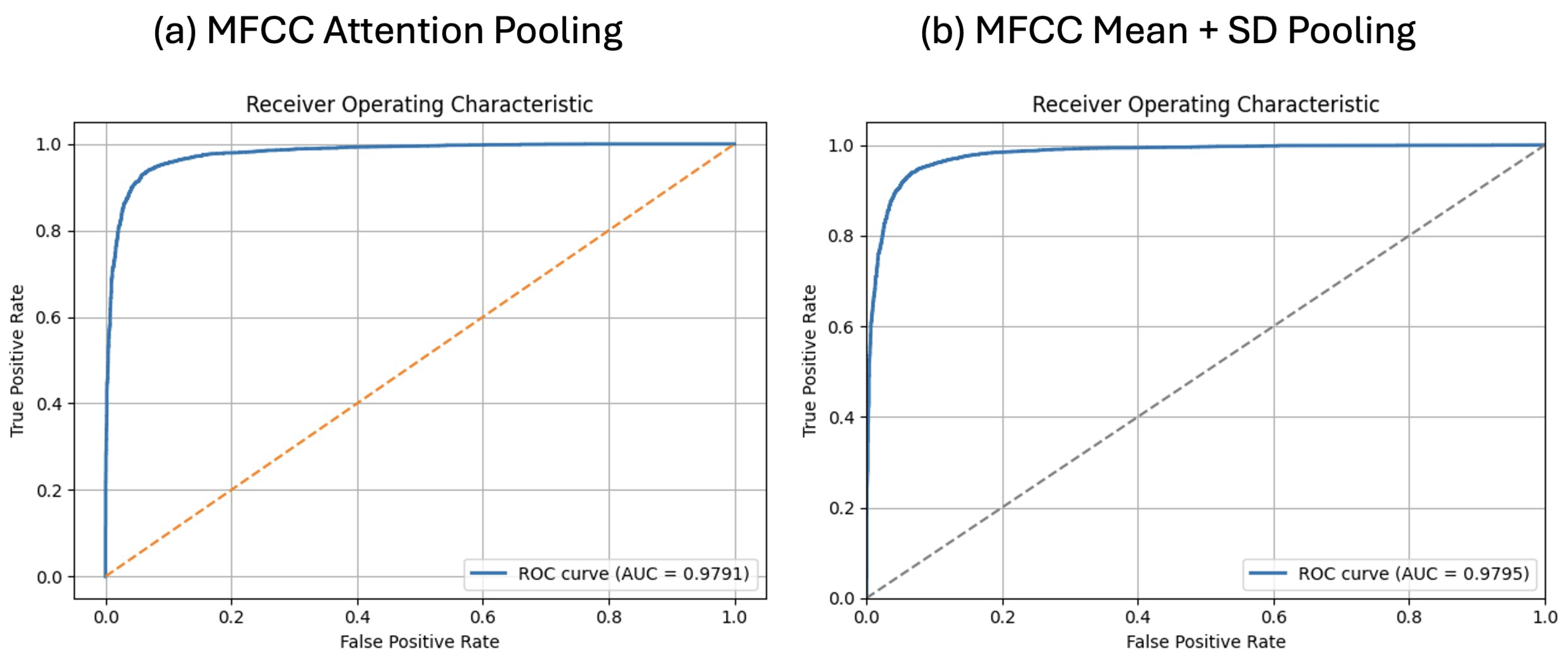
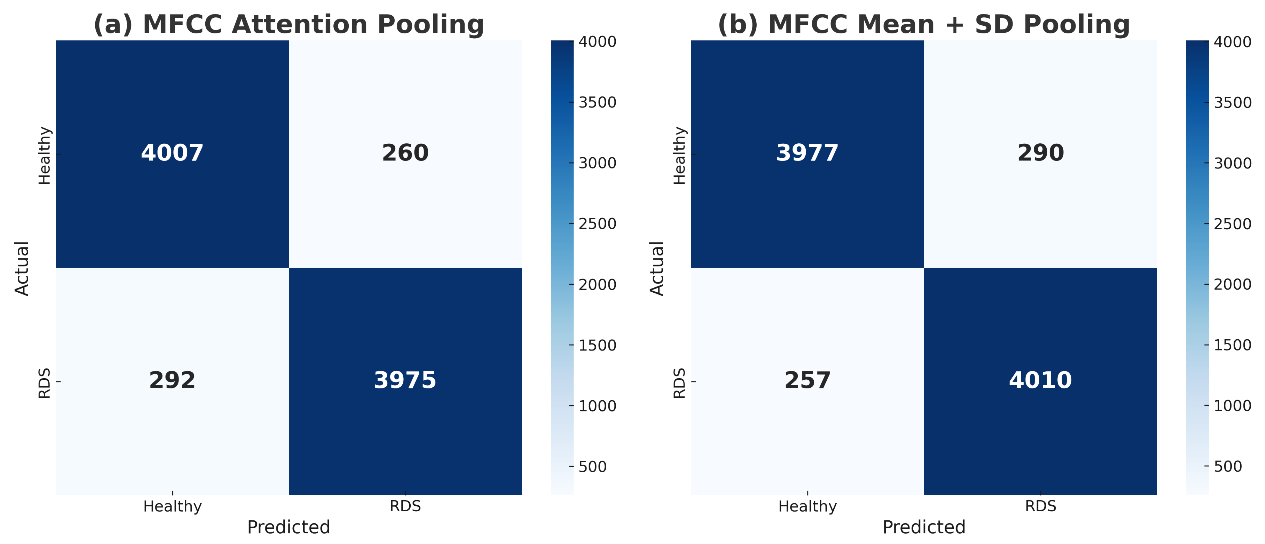
Results in Table 3 show that both pooling strategies achieved comparable performance. The mean–SD pooling model slightly outperformed attention pooling in terms of accuracy (93.59 ± 0.48% vs. 93.53 ± 0.52%), F1-score (93.61 ± 0.50% vs. 93.51 ± 0.52%), and AUC (0.9795 vs. 0.9791). In contrast, attention pooling yielded higher precision (93.87 ± 0.72%), while mean–SD pooling offered better recall (93.98 ± 1.19%). These trade-offs are reflected in the ROC curves (Figure 3) and confusion matrices (Figure 4). As shown, the mean + SD pooling model yields fewer false negatives (257 vs. 292), which is important when missed RDS cases are costly. Conversely, the attention pooling model yields fewer false positives (260 vs. 290), indicating higher specificity and fewer unnecessary alarms.

4.2. FBANK Results with Mean + SD and Attention Pooling

Table 4 demonstrates that while both pooling strategies converged on similar window–hop and FFT settings, their optimal feature and activation choices differed: mean–SD pooling favored fewer mel filters and LeakyReLU, whereas attention pooling favored more mel filters and GELU.
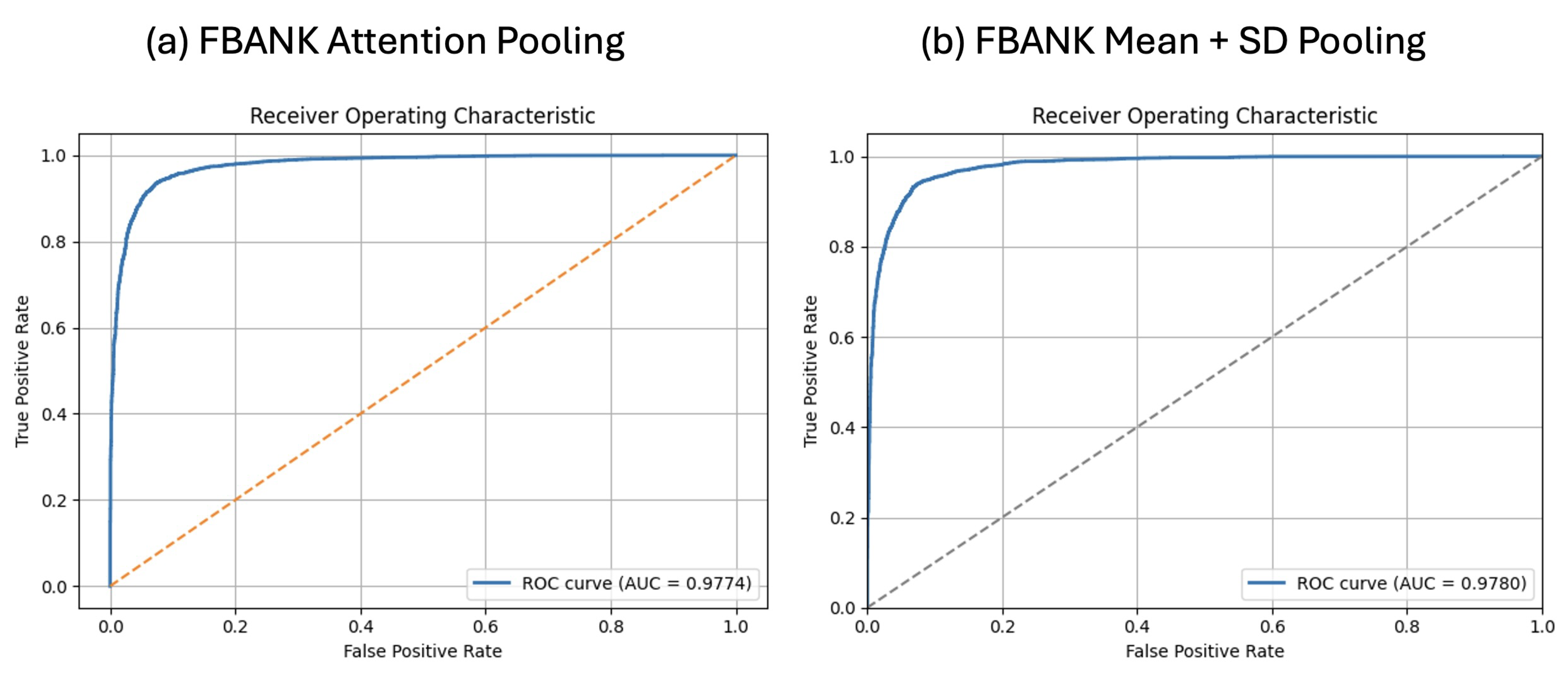
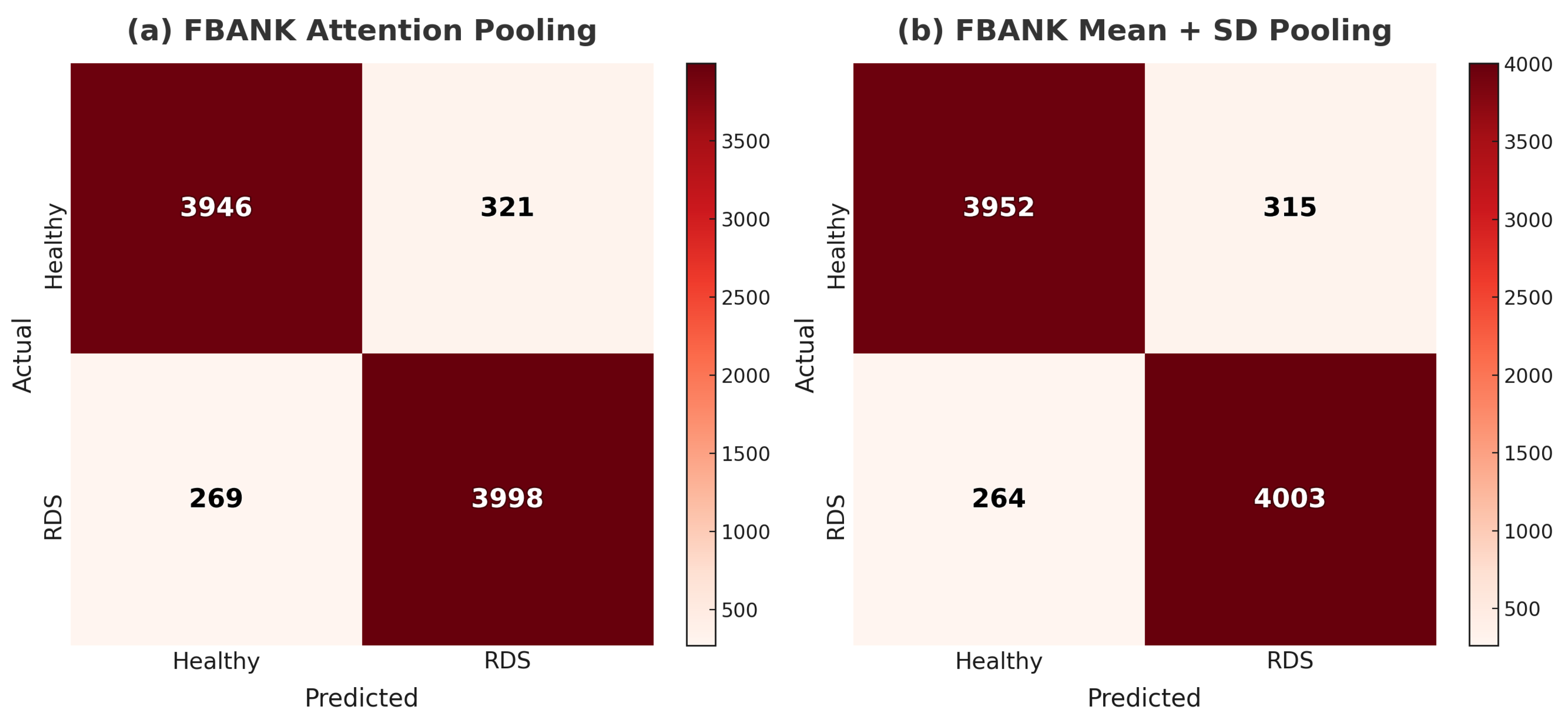
As shown in Table 5, both FBANK-based models achieved similar performance, with mean accuracies of 93.22 ± 0.71% for mean–SD pooling and 93.09 ± 0.84% for attention pooling. The ROC curves in Figure 5 illustrate their comparable discriminative ability, while the confusion matrices in Figure 6 highlight minor differences in error distribution. Attention pooling produced slightly more false negatives (269 vs. 264), whereas mean–SD pooling achieved marginally higher precision and F1-score, consistent with its lower false-positive count (315 vs. 321). Both configurations reached similar AUC values (0.9780 vs. 0.9774), indicating that pooling mainly affects the FP/FN balance rather than overall ranking. Given that RDS (class 1) is the clinically relevant positive class, mean–SD pooling is marginally more favorable due to its lower false-negative rate.

4.3. Interpretability

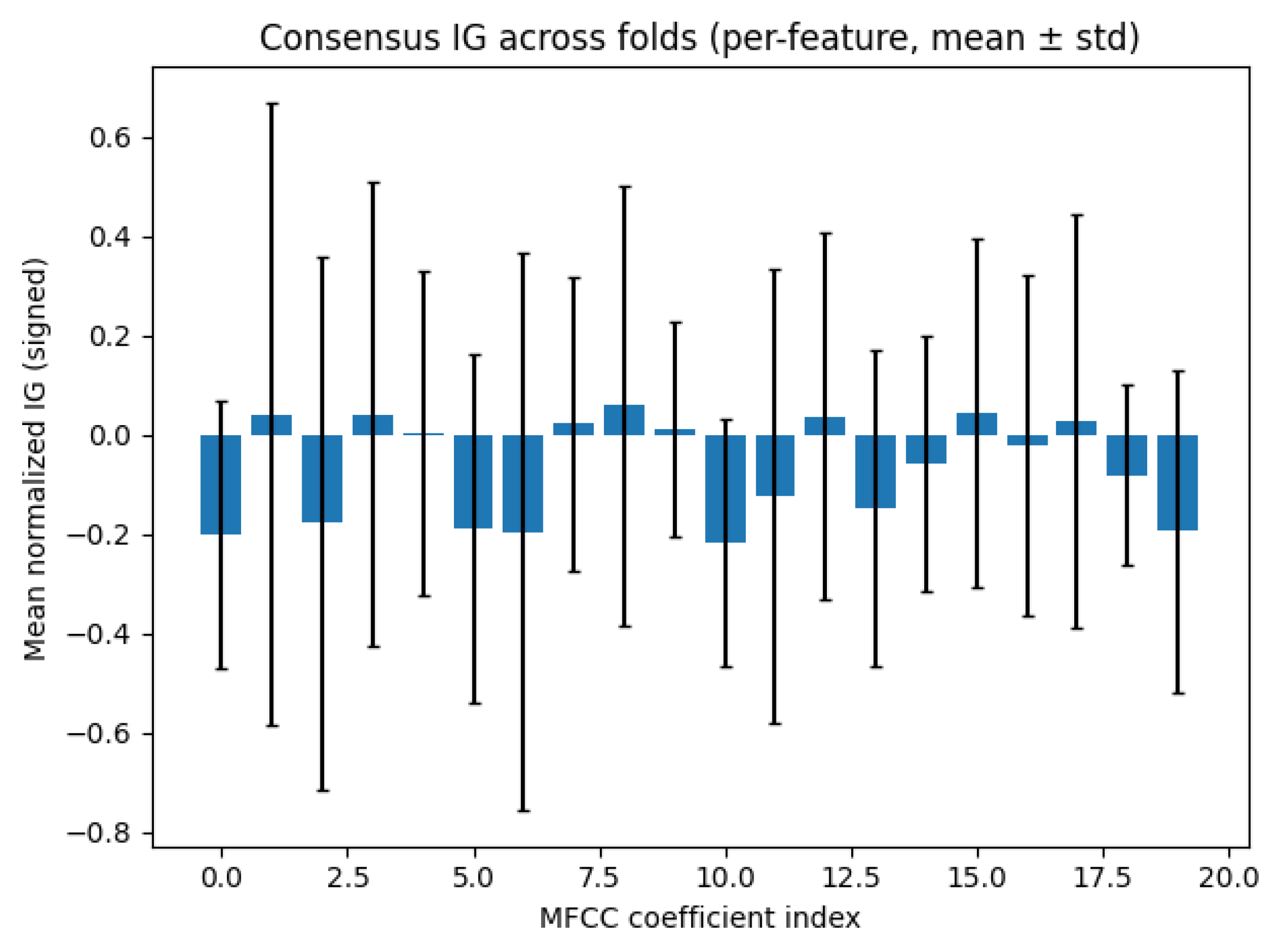
We interpret decisions with IG, attributing the class-1 (RDS) score to MVN-normalized MFCC/FBANK inputs using a zero baseline (MVN mean); per-frame attributions [ T × D ] are summed over time to yield a per-feature profile [ D ] . Under 10-fold cross-validation, we compute one IG vector per fold and report mean ± SD across folds (signed: + = RDS, − = healthy). The IG visualizations in Figure 7 and Figure 8 are taken from the best-performing validation fold (lowest error) of the MFCC with mean + SD pooling configuration—the top MFCC setting in our search (Table 2). In Figure 7, each panel corresponds to the first sample of its fold (illustrative, not a fold average): c2–c4 are often positive (RDS-leaning); c5–c6 negative/near zero (Healthy-leaning); c7–c9 mixed with small effects; c10–c13 consistently negative—especially c12–c13—favoring healthy; c14 variable; c15–c16 positive (RDS-supporting); c17 mixed/slightly negative; and c18–c19 commonly positive (RDS-leaning). The consensus in Figure 8 confirms these tendencies (RDS: c2–c4, c15–c16, and c18–c19; healthy: c10–c13, especially c12–c13); error bars indicate stability (smaller around c12–c13) versus variability (larger at some low/high indices).
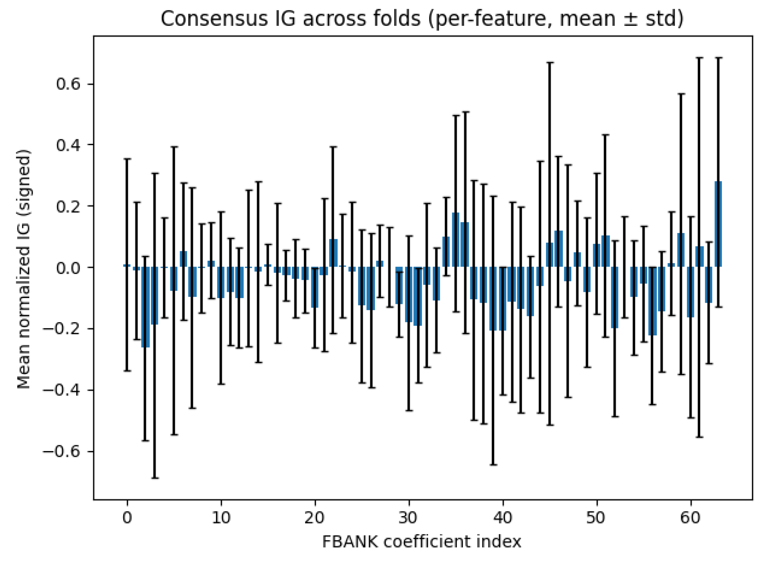
The IG visualizations in Figure 9 and Figure 10 are taken from the best-performing validation fold (lowest error) of the FBANK mean + SD pooling configuration—the top FNANK setting in our search (Table 4). In Figure 9 (per-fold first-sample snapshots), FBANK attributions (signed IG; + for RDS, − for healthy) are weak/mixed in the lowest filters (∼0–10), mostly small or slightly negative in the lower-mid range (∼10–25), and heterogeneous in the mid band (∼25–35). A clear structure emerges in the upper-mid region (∼35–52) with alternating bands—positive spikes around (∼36–46) and near ∼50 (RDS, +) interleaved with nearby negative troughs (healthy, −)—while the highest filters (∼52–63) often show the largest magnitudes (final bins frequently +, adjacent bins sometimes −). The fold-level summary in Figure 10 (mean ± SD across folds) aligns with these patterns: generally small means with notable variability, a weak negative bias in the mid band (∼30–45), and modest positives around (∼36–46) and toward the highest bins (∼60–63). Overall, discriminative evidence concentrates in the upper-mid to high mel range, whereas lower bands contribute more weakly.
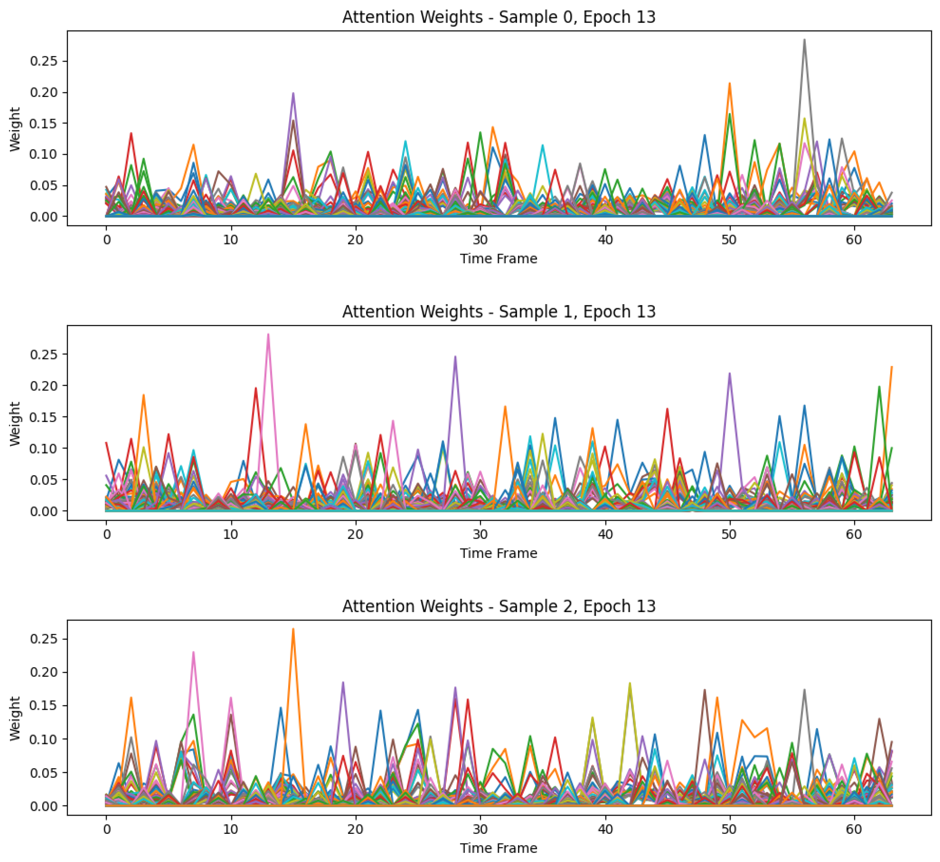
Figure 11 shows the first three validation utterances at epoch 13 for our lightweight X-vector with MFCC inputs and a four-head attention pooling layer, taken from the best-performing validation fold (lowest error) of the MFCC with attention pooling configuration—the top MFCC setting in our search (Table 2). The horizontal axis is the post-TDNN time index ( T = 60 frames for this batch), and the vertical axis is the softmax-normalized attention weight [ 0 , 1 ] . Each colored curve corresponds to one row A q , : (the distribution over key frames for query q). The distributions are distinctly non-uniform, concentrating mass on sparse segments rather than spreading it evenly across MFCC frames—evidence of selective focus on brief informative events. Although pooling uses h = 4 heads, the plot displays head-averaged weights (PyTorch default), so head count does not alter the horizontal axis length; per-head views highlight different frame subsets emphasized by different heads.

4.4. Comparison with Previous Studies

We situate our results alongside prior newborn cry works that include RDS within broader tasks (e.g., sepsis/RDS/healthy) [11,12,13,14] and our earlier binary RDS vs. healthy study on a smaller, full-term-only cohort [10]. Table 6 lists population, size, newborn counts, duration filters, features, and accuracy. Although all studies draw samples from the same underlying database, they use different proportions and subsets and follow different experimental methodologies; therefore, results are not head to head. Ref. [10] reflects contextual prior work (SVM on concatenated MFCC+Tilt+Rhythm). Our proposed method extends that line to a private preterm+full-term cohort with a consistent pipeline, achieving >93% accuracy.

5. Discussion

This study investigated the automatic classification of newborn cries to distinguish between RDS and healthy infants, spanning both preterm and full-term populations. Unlike prior work limited to full-term cohorts, this is the first study to include both subgroups with equal numbers of newborns per class, ensuring balanced representation and reducing bias. Following pre-processing (channel averaging, pre-emphasis filtering, and manual segmentation), expiratory cry segments (EXPs) were extracted as the most diagnostic units, and stratified 10-fold cross-validation was employed to ensure robust and unbiased evaluation. To adapt the X-vector framework to the NCDS, we performed a systematic grid search, training the network under different parameter configurations across three domains—feature extraction, training settings, and model architecture—to identify the values yielding the best overall performance. Based on these optimized parameters, a streamlined lightweight X-vector was trained on two acoustic feature sets (MFCCs and FBANKs) with two pooling strategies (mean–SD and attention), and performance was assessed using accuracy, precision, recall, F1-score, and AUC, complemented by confusion matrices and ROC analysis.
Using MFCC features, both pooling strategies deliver strong, near-identical performance (accuracy ≈ 93.5%, AUC ≈ 0.98). mean + SD is slightly higher in accuracy (93.59 ± 0.48%), recall (93.98 ± 1.19%), F1 (93.61 ± 0.50%), and AUC (0.9795), whereas attention attains higher precision (93.87 ± 0.72% vs. 93.27 ± 0.74%). Consistent with the confusion matrices in Figure 4 and ROC curves, mean + SD yields fewer false negatives (257 vs. 292), prioritizing sensitivity to RDS, while attention yields fewer false positives (260 vs. 290), indicating higher specificity.
Using FBANK features, both pooling strategies perform similarly (accuracy ≈ 93.1–93.2%, AUC ≈ 0.98). mean + SD shows small, consistent gains across metrics—accuracy (93.22 ± 0.71%), precision (92.74 ± 1.48%), recall (93.81 ± 1.31%), F1 (93.26 ± 0.68%), and AUC (0.9780)—relative to attention (93.09 ± 0.84%, 92.57 ± 1.03%, 93.70 ± 0.93%, 93.13 ± 0.83%, 0.9774). Consistent with the confusion matrices in Figure 6, mean + SD yields fewer false negatives (264 vs. 269) and false positives (315 vs. 321), while ROC curves in Figure 5 confirm near-identical ranking performance. Overall, pooling chiefly shifts the FP/FN balance rather than discrimination; given RDS as the positive class, mean + SD is marginally preferable due to its lower miss rate.
Across features, MFCCs outperform FBANKs (best MFCC: 93.59% accuracy, AUC = 0.9795; best FBANK: 93.22% accuracy, AUC = 0.9780), indicating the diagnostic value of cepstral representations for RDS. For pooling, effects are small but consistent: with MFCCs, mean + SD is slightly higher in accuracy, recall, F1, and AUC and yields fewer missed RDS cases (false negatives: 257 vs. 292 for attention), whereas attention offers higher precision and fewer false alarms (false positives: 260 vs. 290). With FBANKs, mean + SD shows small gains across metrics and produces both fewer false negatives (264 vs. 269) and fewer false positives (315 vs. 321) than attention. An ablation on depth showed that increasing the TDNN from five to seven layers (with narrower channels and staged dilations) produced small but consistent gains in accuracy and AUC under the same 10-fold protocol; therefore, we use the seven-layer lightweight design throughout. From a computational standpoint, the MFCC attention model has 641.2 k trainable parameters versus 441.6 k for MFCC mean + SD (Table A1), i.e., about 45% fewer parameters for mean + SD with slightly better overall discrimination. In practice, if minimizing missed RDS cases is the priority, MFCC with mean + SD is preferable; if reducing false alarms is more important, MFCC with attention may be chosen, acknowledging the higher parameter count. Previous cry-based studies achieved high accuracies (up to 98.7%) but were restricted to full-term infants and often relied on imbalanced or underspecified datasets [10,11,12,13]. In contrast, our dataset is larger, demographically diverse, and subject-balanced across preterm and full-term infants, directly addressing the limitations of earlier work. The inclusion of preterm cries, which are acoustically less stable—featuring higher pitch variability, flatter contours, and shorter, noisier bursts—introduces additional classification challenges. Despite this, our framework achieved 93.6% accuracy, reflecting a more realistic and generalizable scenario than prior full-term-only studies. Furthermore, unlike earlier approaches, our method employs a lightweight, optimized X-vector with attention pooling and integrates interpretability via attention maps and Integrated Gradients, advancing both efficiency and clinical trust.
While the proposed framework demonstrates strong performance, there remains room for further advancement. Future work should investigate advanced signal processing features—particularly from the cepstral domain—to more effectively capture the distinct acoustic characteristics of preterm and full-term cries. In addition, developing models explicitly designed for variable-length inputs will be essential to ensure robust and reliable evaluation across diverse recording conditions. A further limitation is the reliance on manual annotation-based segmentation, which, while ensuring accurate extraction of expiratory segments, introduces subjectivity and limits scalability. Future research should pursue automated segmentation to enhance reproducibility and enable broader clinical application.
This study demonstrates the feasibility of combining cepstral features, a lightweight optimized X-vector, and attention pooling within a balanced dataset for cry-based disease classification. By uniting strong performance with interpretability and scalability, the framework establishes a solid foundation for future work to refine feature representations and design more sophisticated models aimed at improving diagnostic accuracy and ultimately advancing neonatal care.

Author Contributions

Conceptualization, S.V.S. and C.T.; data curation, S.V.S.; formal analysis, S.V.S.; investigation, S.V.S.; methodology, S.V.S. and C.T.; project administration, C.T.; resources, C.T.; software, S.V.S.; supervision, C.T.; validation, S.V.S.; visualization, S.V.S.; writing—original draft, S.V.S.; writing—review and editing, S.V.S. and C.T. All authors have read and agreed to the published version of the manuscript.

Funding

This research received no external funding.

Institutional Review Board Statement

The study was conducted according to the guidelines of the Declaration of Helsinki and approved by the Ethics Committee of École de Technologie Supérieure (#H20100401). Approval date: 4 March 2022.

Informed Consent Statement

Informed consent was obtained from all subjects involved in the study.

Data Availability Statement

Data supporting the reported results are not publicly available due to privacy and ethical restrictions.

Conflicts of Interest

The authors declare no conflicts of interest.

Appendix A. Comparison of X-Vector Architectures

Given their near-identical performance (Acc.: 93.59 ± 0.48 vs. 93.53 ± 0.52 ; Table 3), we report both lightweight-modified X-vector (MFCC, mean + SD) and (MFCC, attention). Compared with the original X-vector, which uses five TDNN layers with fixed dilation and statistics pooling, the lightweight designs adopt seven TDNN layers with reduced channels and variable dilation, using either four-head self-attention pooling (attention) or statistics pooling with a 512 256 projection (mean + SD). They are also dramatically smaller: ∼0.642 M (attention) and 0.442 M (mean + SD) parameters versus ∼8.7 M for the original—about 14– 20 × fewer (Table A1).
Table A1. Comparison between the original X-vector architecture and the lightweight-modified versions used in this study.
ComponentOriginal X-Vector [31]Lightweight-Modified X-Vector (MFCC, Attention)Lightweight-Modified X-Vector (MFCC, Mean + SD)
Input FeaturesMFCCs (typically 23–30 dims)MFCCMFCC
Input Channels∼3026 MFCCs20 MFCCs
TDNN Stack5 TDNN layers, fixed dilation7 TDNN layers, reduced channels with variable dilation7 TDNN layers, reduced channels with variable dilation
TDNN Channels[512, 512, 512, 512, 1500][64, 64, 128, 128, 128, 256, 256][64, 64, 128, 128, 128, 256, 256]
TDNN Kernel Sizes[5, 5, 7, 9, 1][5, 3, 3, 3, 3, 1, 1][5, 3, 3, 3, 3, 1, 1]
TDNN Dilations[1, 1, 1, 1, 1][1, 1, 2, 2, 3, 1, 1][1, 1, 2, 2, 3, 1, 1]
Activation FunctionReLUGELULeakyReLU ( α = 0.01 )
NormalizationBatchNorm after each TDNN and dense blockSameSame
PoolingStatistics pooling (mean and std over time)4-head self-attention with maskingStatistics pooling (mean and std over time)
Embedding Dimension512 (after pooling)256 (after pooling and linear projection)256 (after pooling and linear projection)
Fully Connected LayersFC1: 512, FC2: 1500FC1: 256, FC2: 256FC1: 256, FC2: 256
Backend / ClassifierPLDA scoringFeedforward classifier + Sigmoid outputFeedforward classifier
+ Softmax output
Total Trainable Parameters∼8.7 M641.2 k441.6 k
Inference Latency Per 1 s
Segment (A100, batch = 64)
∼5.5 ms/segment (∼181 seg/s; real-time × 180)∼6–7 ms/segment (estimated)

References

  1. UNICEF. Neonatal Mortality – UNICEF Data. UNICEF Data Portal. 2024. Available online: https://data.unicef.org/topic/child-survival/neonatal-mortality/ (accessed on 21 July 2025).
  2. UNICEF. Levels and Trends in Child Mortality: Report 2024. UNICEF Data Portal. 2024. Available online: https://data.unicef.org/resources/levels-and-trends-in-child-mortality-2024/ (accessed on 21 July 2025).
  3. World Health Organization (WHO). Neonatal Mortality Rate (per 1000 Live Births). WHO Global Health Observatory. 2024. Available online: https://data.who.int/indicators/i/E3CAF2B/A4C49D3 (accessed on 21 July 2025).
  4. Tochie, J.N.; Chuy, C.; Shalkowich, T.; Olayinka, O.O.; Tanveer, M.; Dondorp, A.M.; Kreuels, B.; Mayhew, S.; Dramowski, A. Global, Regional, and National Trends in the Burden of Neonatal Respiratory Failure: A Scoping Review from 1992 to 2022. J. Clin. Transl. Res. 2023, 8, 637–649. [Google Scholar]
  5. Legesse, B.; Cherie, A.; Wakwoya, E. Time to Death and Its Predictors Among Neonates with Respiratory Distress Syndrome Admitted at Public Hospitals in Addis Ababa, Ethiopia, 2019–2021: A Retrospective Cohort Study. PLoS ONE 2023, 18, e0289050. [Google Scholar]
  6. Wasz-Höckert, O.; Valanne, E.; Michelsson, K.; Vuorenkoski, V.; Lind, J. Twenty-Five Years of Scandinavian Cry Research. In Infant Crying: Theoretical and Research Perspectives; Lester, B.M., Boukydis, C.F.Z., Eds.; Plenum Press: New York, NY, USA, 1984; pp. 83–94. [Google Scholar]
  7. Mukhopadhyay, J.; Saha, B.; Majumdar, B.; Majumdar, A.; Gorain, S.; Arya, B.K.; Bhattacharya, S.D.; Singh, A. An Evaluation of Human Perception for Neonatal Cry Using a Database of Cry and Underlying Cause. In Proceedings of the 2013 Indian Conference on Medical Informatics and Telemedicine (ICMIT), Kharagpur, India, 28–30 March 2013; pp. 64–67. [Google Scholar]
  8. Owino, G.; Shibwabo, B. Advances in Infant Cry Paralinguistic Classification—Methods, Implementation, and Applications: Systematic Review. JMIR Rehabil. Assist. Technol. 2025, 12, e69457. [Google Scholar] [CrossRef]
  9. Ji, C.; Mudiyanselage, T.B.; Gao, Y.; Pan, Y. A Review of Infant Cry Analysis and Classification. EURASIP J. Audio Speech Music Process. 2021, 2021, 8. [Google Scholar] [CrossRef]
  10. Matikolaie, F.S.; Tadj, C. On the Use of Long-Term Features in a Newborn Cry Diagnostic System. Biomed. Signal Process. Control 2020, 59, 101889. [Google Scholar]
  11. Zayed, Y.; Hasasneh, A.; Tadj, C. Infant Cry Signal Diagnostic System Using Deep Learning and Fused Features. Diagnostics 2023, 13, 2107. [Google Scholar] [CrossRef]
  12. Mohammad, A.; Tadj, C. Transformer-Based Approach to Pathology Diagnosis Using Audio Spectrograms. J. Pathol. Audio Diagn. 2024, 1, 45–58. [Google Scholar]
  13. Masri, S.; Hasasneh, A.; Tami, M.; Tadj, C. Exploring the Impact of Image-Based Audio Representations in Classification Tasks Using Vision Transformers and Explainable AI Techniques. Information 2024, 15, 751. [Google Scholar] [CrossRef]
  14. Shayegh, S.V.; Tadj, C. Deep Audio Features and Self-Supervised Learning for Early Diagnosis of Neonatal Diseases: Sepsis and Respiratory Distress Syndrome Classification from Infant Cry Signals. Electronics 2025, 14, 248. [Google Scholar] [CrossRef]
  15. Pardede, H.F.; Zilvan, V.; Krisnandi, D.; Heryana, A.; Kusumo, R.B.S. Generalized Filter-Bank Features for Robust Speech Recognition Against Reverberation. In Proceedings of the 2019 International Conference on Computer, Control, Informatics and Its Applications (IC3INA), Tangerang, Indonesia, 23–24 October 2019; pp. 19–24. [Google Scholar]
  16. Mukherjee, H.; Salam, H.; Santosh, K.C. Lung Health Analysis: Adventitious Respiratory Sound Classification Using Filterbank Energies. Int. J. Pattern Recognit. Artif. Intell. 2021, 35, 2157008. [Google Scholar] [CrossRef]
  17. Tak, R.N.; Agrawal, D.M.; Patil, H.A. Novel Phase Encoded Mel Filterbank Energies for Environmental Sound Classification. In Proceedings of the 7th International Conference on Pattern Recognition and Machine Intelligence (PReMI 2017), Kolkata, India, 5–8 December 2017; pp. 317–325. [Google Scholar]
  18. Salehian Matikolaie, F.; Kheddache, Y.; Tadj, C. Automated Newborn Cry Diagnostic System Using Machine Learning Approach. Biomed. Signal Process. Control 2022, 73, 103434. [Google Scholar] [CrossRef]
  19. Khalilzad, Z.; Tadj, C. Using CCA-Fused Cepstral Features in a Deep Learning-Based Cry Diagnostic System for Detecting an Ensemble of Pathologies in Newborns. Diagnostics 2023, 13, 879. [Google Scholar] [CrossRef] [PubMed]
  20. Patil, H.A.; Patil, A.T.; Kachhi, A. Constant Q Cepstral Coefficients for Classification of Normal vs. Pathological Infant Cry. In Proceedings of the ICASSP 2022—IEEE International Conference on Acoustics, Speech and Signal Processing, Singapore, 22–27 May 2022; pp. 7392–7396. [Google Scholar]
  21. Felipe, G.Z.; Aguiar, R.L.; Costa, Y.M.G.; Silla, C.N.; Brahnam, S.; Nanni, L.; McMurtrey, S. Identification of Infants’ Cry Motivation Using Spectrograms. In Proceedings of the 2019 International Conference on Systems, Signals and Image Processing (IWSSIP), Osijek, Croatia, 5–7 June 2019; pp. 181–186. [Google Scholar]
  22. Farsaie Alaie, H.; Abou-Abbas, L.; Tadj, C. Cry-Based Infant Pathology Classification Using GMMs. Speech Commun. 2016, 77, 28–52. [Google Scholar] [CrossRef]
  23. Salehian Matikolaie, F.; Tadj, C. Machine Learning-Based Cry Diagnostic System for Identifying Septic Newborns. J. Voice 2024, 38, 963.e1–963.e14. [Google Scholar] [CrossRef]
  24. Zabidi, A.; Yassin, I.M.; Hassan, H.A.; Ismail, N.; Hamzah, M.M.A.M.; Rizman, Z.I.; Abidin, H.Z. Detection of Asphyxia in Infants Using Deep Learning Convolutional Neural Network (CNN) Trained on Mel Frequency Cepstrum Coefficient (MFCC) Features Extracted from Cry Sounds. J. Fundam. Appl. Sci. 2018, 9, 768. [Google Scholar] [CrossRef]
  25. Ting, H.-N.; Choo, Y.-M.; Ahmad Kamar, A. Classification of Asphyxia Infant Cry Using Hybrid Speech Features and Deep Learning Models. Expert Syst. Appl. 2022, 208, 118064. [Google Scholar] [CrossRef]
  26. Ji, C.; Xiao, X.; Basodi, S.; Pan, Y. Deep Learning for Asphyxiated Infant Cry Classification Based on Acoustic Features and Weighted Prosodic Features. In Proceedings of the 2019 International Conference on Internet of Things (iThings), IEEE Green Computing and Communications (GreenCom), IEEE Cyber, Physical and Social Computing (CPSCom), and IEEE Smart Data (SmartData), Atlanta, GA, USA, 14–17 July 2019; pp. 1233–1240. [Google Scholar]
  27. Wu, K.; Zhang, C.; Wu, X.; Wu, D.; Niu, X. Research on Acoustic Feature Extraction of Crying for Early Screening of Children with Autism. In Proceedings of the 2019 34rd Youth Academic Annual Conference of Chinese Association of Automation (YAC), Guilin, China, 18–20 May 2019; pp. 290–295. [Google Scholar]
  28. Satar, M.; Cengizler, Ç.; Hamitoğlu, Ş.; Özdemir, M. Audio Analysis Based Diagnosis of Hypoxic Ischemic Encephalopathy in Newborns. Int. J. Adv. Biomed. Eng. 2022, 1, 28–42. [Google Scholar]
  29. Reyes-Galaviz, O.F.; Tirado, E.A.; Reyes-Garcia, C.A. Classification of Infant Crying to Identify Pathologies in Recently Born Babies with ANFIS. In Proceedings of the International Conference on Computers Helping People with Special Needs (ICCHP 2004), Paris, France, 7–9 July 2004; Lecture Notes in Computer Science, Volume 3118. pp. 408–415. [Google Scholar]
  30. Hariharan, M.; Sindhu, R.; Vijean, V.; Yazid, H.; Nadarajaw, T.; Yaacob, S.; Polat, K. Improved Binary Dragonfly Optimization Algorithm and Wavelet Packet Based Non-Linear Features for Infant Cry Classification. Comput. Methods Programs Biomed. 2018, 155, 39–51. [Google Scholar] [CrossRef]
  31. Snyder, D.; Garcia-Romero, D.; Sell, G.; Povey, D.; Khudanpur, S. X-Vectors: Robust DNN Embeddings for Speaker Recognition. In Proceedings of the IEEE International Conference on Acoustics, Speech and Signal Processing (ICASSP 2018), Calgary, AB, Canada, 15–20 April 2018; pp. 5329–5333. [Google Scholar]
  32. Snyder, D.; Garcia-Romero, D.; Sell, G.; McCree, A.; Povey, D.; Khudanpur, S. Speaker Recognition for Multi-Speaker Conversations Using X-Vectors. In Proceedings of the IEEE International Conference on Acoustics, Speech and Signal Processing (ICASSP 2019), Brighton, UK, 12–17 May 2019; pp. 5796–5800. [Google Scholar]
  33. Snyder, D.; Garcia-Romero, D.; McCree, A.; Sell, G.; Povey, D.; Khudanpur, S. Spoken Language Recognition Using X-Vectors. In Proceedings of the Odyssey 2018: The Speaker & Language Recognition Workshop, Les Sables d’Olonne, France, 26–29 June 2018; pp. 105–111. [Google Scholar]
  34. Novotný, O.; Matejka, P.; Cernocký, J.; Burget, L.; Glembek, O. On the Use of X-Vectors for Robust Speaker Recognition. In Proceedings of the Odyssey 2018: The Speaker & Language Recognition Workshop, Les Sables d’Olonne, France, 26–29 June 2018; pp. 111–118. [Google Scholar]
  35. Karafiát, M.; Veselý, K.; Černocký, J.; Profant, J.; Nytra, J.; Hlaváček, M.; Pavlíček, T. Analysis of X-Vectors for Low-Resource Speech Recognition. In Proceedings of the IEEE International Conference on Acoustics, Speech and Signal Processing (ICASSP 2021), Toronto, ON, Canada, 6–11 June 2021; pp. 6998–7002. [Google Scholar]
  36. Zeinali, H.; Burget, L.; Černocký, J. Convolutional Neural Networks and X-Vector Embedding for DCASE2018 Acoustic Scene Classification Challenge. In Proceedings of the Detection and Classification of Acoustic Scenes and Events 2018 Workshop (DCASE2018), Surrey, UK, 19–20 November 2018; pp. 202–206. [Google Scholar]
  37. Janský, J.; Málek, J.; Čmejla, J.; Kounovský, T.; Koldovský, Z.; Žďánský, J. Adaptive Blind Audio Source Extraction Supervised by Dominant Speaker Identification Using X-Vectors. In Proceedings of the IEEE International Conference on Acoustics, Speech and Signal Processing (ICASSP 2020), Barcelona, Spain, 4–8 May 2020; pp. 676–680. [Google Scholar]
  38. Michelsson, K.; Järvenpää, A.L.; Rinne, A. Sound Spectrographic Analysis of Pain Cry in Preterm Infants. Early Hum. Dev. 1983, 8, 141–149. [Google Scholar] [CrossRef]
  39. Lester, B.M.; Boukydis, C.F.Z.; Garcia-Coll, C. Neonatal Cry Analysis and Risk Assessment. In Newborn Behavioral Organization and the Assessment of Risk; Lester, B.M., Boukydis, C.F.Z., Eds.; Cambridge University Press: Cambridge, UK, 1992; pp. 137–158. [Google Scholar]
  40. Mampe, B.; Friederici, A.D.; Christophe, A.; Wermke, K. Newborns’ Cry Melody Is Shaped by Their Native Language. Curr. Biol. 2009, 19, 1994–1997. [Google Scholar] [CrossRef] [PubMed]
  41. Lind, K.; Wermke, K. Development of the Vocal Fundamental Frequency of Spontaneous Cries during the First 3 Months. Int. J. Pediatr. Otorhinolaryngol. 2002, 64, 97–104. [Google Scholar] [CrossRef]
  42. Boukydis, C.Z.; Lester, B.M. Infant Crying: Theoretical and Research Perspectives; Plenum Press: New York, NY, USA, 1985. [Google Scholar]
  43. Kohavi, R. A Study of Cross-Validation and Bootstrap for Accuracy Estimation and Model Selection. In Proceedings of the 14th International Joint Conference on Artificial Intelligence (IJCAI), Montreal, QC, Canada, 20–25 August 1995; pp. 1137–1143. [Google Scholar]
  44. Young, S.; Evermann, G.; Gales, M.; Hain, T.; Kershaw, D.; Liu, X.; Moore, G.; Odell, J.; Ollason, D.; Povey, D.; et al. The HTK Book (for HTK Version 3.4); Cambridge University Engineering Department: Cambridge, UK, 2006. [Google Scholar]
  45. Davis, S.; Mermelstein, P. Comparison of parametric representations for monosyllabic word recognition in continuously spoken sentences. IEEE Trans. Acoust. Speech Signal Process. 1980, 28, 357–366. [Google Scholar] [CrossRef]
  46. Waibel, A.; Hanazawa, T.; Hinton, G.; Shikano, K.; Lang, K.J. Phoneme Recognition Using Time-Delay Neural Networks. IEEE Trans. Acoust. Speech Signal Process. 1989, 37, 328–339. [Google Scholar] [CrossRef]
  47. Vaswani, A.; Shazeer, N.; Parmar, N.; Uszkoreit, J.; Jones, L.; Gomez, A.N.; Kaiser, Ł.; Polosukhin, I. Attention Is All You Need. arXiv 2017, arXiv:1706.03762. [Google Scholar]
  48. Okabe, K.; Koshinaka, T.; Shinoda, K. Attentive Statistics Pooling for Deep Speaker Embedding. In Proceedings of the Annual Conference of the International Speech Communication Association (Interspeech), Hyderabad, India, 2–6 September 2018; pp. 2252–2256. [Google Scholar]
  49. Paszke, A.; Gross, S.; Massa, F.; Lerer, A.; Bradbury, J.; Chanan, G.; Killeen, T.; Lin, Z.; Gimelshein, N.; Antiga, L.; et al. PyTorch: An Imperative Style, High-Performance Deep Learning Library. Available online: https://pytorch.org/ (accessed on 5 September 2025).
  50. Sundararajan, M.; Taly, A.; Yan, Q. Axiomatic attribution for deep networks. In Proceedings of the 34th International Conference on Machine Learning (ICML), Exeter, UK, 21–23 June 2017; Volume 70, pp. 3319–3328. [Google Scholar]
  51. Fawcett, T. An Introduction to ROC Analysis. Pattern Recogn. Lett. 2006, 27, 861–874. [Google Scholar] [CrossRef]
  52. Bradley, A.P. The Use of the Area Under the ROC Curve in the Evaluation of Machine Learning Algorithms. Pattern Recogn. 1997, 30, 1145–1159. [Google Scholar] [CrossRef]
  53. Tjoa, E.; Guan, C. A Survey on Explainable Artificial Intelligence (XAI): Toward Medical XAI. IEEE Trans. Neural Netw. Learn. Syst. 2020, 32, 4793–4813. [Google Scholar] [CrossRef]
  54. Digital Research Alliance of Canada. Narval Supercomputing Cluster. Available online: https://alliancecan.ca/en/services/advanced-research-computing/narval (accessed on 5 September 2025).
  55. Yang, Y.-Y.; Hira, M.; Ni, Z.; Chourdia, A.; Astafurov, A.; Chen, C.; Yeh, C.-F.; Puhrsch, C.; Pollack, D.; Genzel, D.; et al. TorchAudio: An Audio Library for PyTorch. Available online: https://pytorch.org/audio/ (accessed on 5 September 2025).
  56. McFee, B.; Raffel, C.; Liang, D.; Ellis, D.P.W.; McVicar, M.; Battenberg, E.; Nieto, O. librosa: Audio and Music Signal Analysis in Python. In Proceedings of the 14th Python in Science Conference, Austin, TX, USA, 6–12 July 2015; pp. 18–24. Available online: https://librosa.org/ (accessed on 5 September 2025).
  57. Ravanelli, M.; Parcollet, T.; Plantinga, P.; Rouhe, A.; Cornell, S.; Lugosch, L.; Subakan, C.; Dawalatabad, N.; Heba, A.; Zhong, J.; et al. SpeechBrain: A General-Purpose Speech Toolkit. arXiv 2021, arXiv:2106.04624. [Google Scholar]
  58. Ravanelli, M.; Parcollet, T.; Moumen, A.; de Langen, S.; Subakan, C.; Plantinga, P.; Wang, Y.; Mousavi, P.; Della Libera, L.; Ploujnikov, A.; et al. Open-Source Conversational AI with SpeechBrain 1.0. arXiv 2024, arXiv:2407.00463. [Google Scholar]
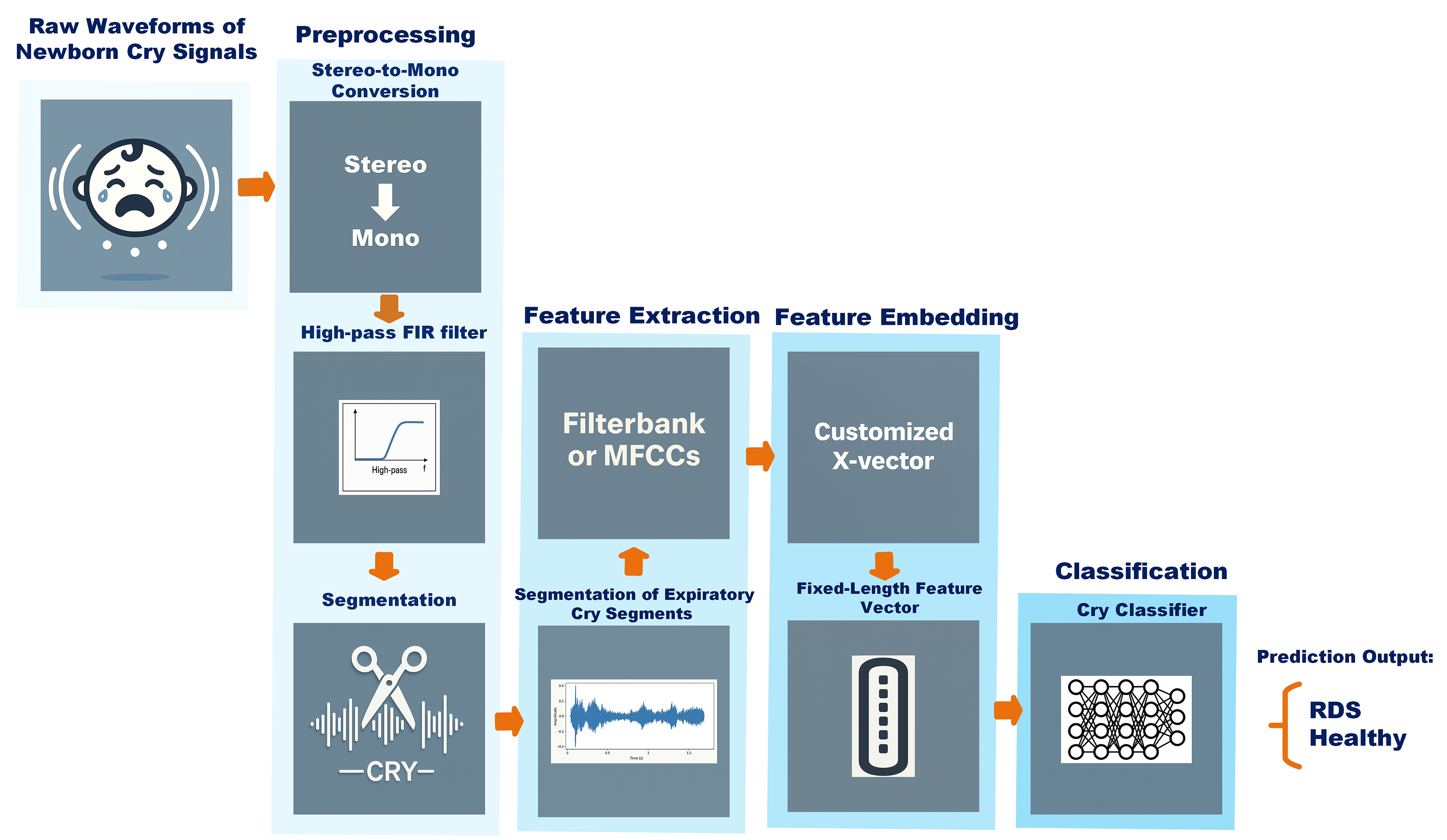
Figure 1. Overview of the proposed NCDS, including pre-processing, feature extraction, feature embedding, and RDS prediction.
Information 16 01008 g001
Figure 2. Extraction of FBANKs and MFCCs from raw baby cry signals, illustrating transitions through time, spectral, and cepstral domains.
Information 16 01008 g002
Figure 3. ROC curves of the X-vector with MFCC features: (a) attention pooling and (b) mean + SD pooling, with AUC values for healthy vs. RDS classification.
Information 16 01008 g003
Figure 4. Confusion matrices of the X-vector with MFCC features: (a) attention pooling and (b) mean + SD pooling, showing classifications of healthy vs. RDS.
Information 16 01008 g004
Figure 5. ROC curves of the X-vector with FBANK features: (a) attention pooling and (b) mean + SD pooling, with AUC values for healthy vs. RDS classification.
Information 16 01008 g005
Figure 6. Confusion matrices of the X-vector with FBANK features: (a) attention pooling and (b) mean + SD pooling, showing classifications of healthy vs. RDS.
Information 16 01008 g006
Figure 7. Per-fold MFCC IG (20 MFCCs, folds 0–9; statistics pooling). One validation utterance per panel. Bars are signed and per-utterance normalized (+ = RDS, − = healthy); On average, c2–c4 and c15–c19 are RDS-leaning, whereas c10–c13 (esp. c12–c13) favor healthy; error bars indicate between-fold variability.
Information 16 01008 g007
Figure 8. Consensus MFCC IG across 10 folds (statistics pooling). Values are signed and per-utterance normalized (+ = RDS, − = healthy). On average, c2–c4 and c15–c19 are RDS-leaning, while c10–c13 (esp. c12–c13) favor healthy; error bars show between-fold variability.
Information 16 01008 g008
Figure 9. Per-fold FBANK IG (80 mel bands; folds 0–9; statistics pooling). One validation utterance per panel; bars are signed and per-utterance normalized (+ = RDS, − = healthy).
Information 16 01008 g009
Figure 10. Consensus FBANK IG across 10 folds (statistics pooling). Values are signed and per-utterance normalized (+ = RDS, − = healthy). Overall, discriminative evidence concentrates in the upper-mid to high mel range, whereas lower bands contribute more weakly.
Information 16 01008 g010
Figure 11. Head-averaged attention weights for three validation utterances at epoch 13 from an MFCC X-vector with 4-head attention pooling. Each color represents a distinct attention weight applied within the attention pooling layer.
Information 16 01008 g011
Table 1. Dataset summary and participant information.
LabelRDSHealthy
No. of Newborns3838
No. of CASs9398
No. of EXPs43174267
Sampling Frequency44.1 kHz44.1 kHz
Duration Range (seconds)[0.040–5.495][0.040–6.184]
Total Duration (seconds)3350.01503332.2570
Table 2. Hyperparameters and optimal values for MFCC experiments under mean + SD and attention pooling. Tested ranges follow standard speech practice and small pilot runs; see Section 3.6 for rationale.
HyperparameterTested ValuesOptimal (Mean + SD)Optimal (Attention)
Feature Extraction Parameters
Window, hop length (ms)[(10, 3), (15, 5), (20, 6), (25, 10)](20, 6)(20, 6)
FFT size[1024, 2048, 4096]20482048
Number of mel filters[30, 40, 64, 80]8080
Number of MFCC coefficients[13, 20, 26]2026
Deltas[True, False]FalseFalse
Filter shape[triangular, gaussian]triangulartriangular
Training Configuration
Learning rate[2.5 × 10⁻⁴, 5 × 10⁻⁴]
(step: 0.5 × 10⁻⁵)
4.5 × 10−44.5 × 10−4
Number of epochs[10, 12, 14]1414
Batch size[16, 32, 64, 128]6464
Weight decay[ 1 × 10 5 , 1 × 10 4 , 1 × 10 3 ] 10 5 10 5
Model Architecture
Activation function[GELU, SiLU (Swish), ReLU, LeakyReLU]LeakyReLUGELU
Type of pooling[Mean + SD, Attention]Mean + SDAttention
Number of attention heads[1, 2, 4, 8]-4
Table 3. Classification performance across 10-fold cross-validation for modified X-vector models using MFCCs.
ModelAccuracyPrecisionRecallF1 ScoreAUC
X-vector MFCC + Mean + SD93.59 ± 0.48%93.27 ± 0.74%93.98 ± 1.19%93.61 ± 0.50%0.9795
X-vector MFCC + Attention93.53 ± 0.52%93.87 ± 0.72%93.16 ± 0.72%93.51 ± 0.52%0.9791
Note: Performance metrics are reported as mean ± standard deviation across 10 folds of cross-validation.
Table 4. Hyperparameters and optimal values for FBANK experiments under mean + SD and attention pooling. Tested ranges follow standard speech practice and small pilot runs; see Section 3.6 for rationale.
HyperparameterTested ValuesOptimal (Mean + SD)Optimal (Attention)
Feature Extraction Parameters
Window, hop length (ms)[(10, 3), (15, 5), (20, 6), (25, 10)](20, 6)(20, 6)
FFT size[1024, 2048, 4096]20482048
Number of mel filters[30, 40, 64, 80]6480
Deltas[True, False]FalseFalse
Filter shape[triangular, Gaussian]triangulartriangular
Training Configuration
Learning rate[2.5 × 10⁻⁴, 5 × 10⁻⁴] (step: 0.5 × 10⁻⁵)5 × 10−44.5 × 10−4
Number of epochs[10, 12, 14]1214
Batch size[16, 32, 64, 128]6464
Weight decay[ 1 × 10 5 , 1 × 10 4 , 1 × 10 3 ] 10 5 10 5
Model Architecture
Activation function[GELU, SiLU (Swish), ReLU, LeakyReLU]LeakyReLUGELU
Type of pooling[Mean + SD, Attention]Mean + SDAttention
Number of attention heads[1, 2, 4, 8]-4
Table 5. Classification performance across 10-fold cross-validation for modified X-vector models using FBANKs.
ModelAccuracyPrecisionRecallF1 ScoreAUC
X-vector FBANK + Mean + SD93.22 ± 0.71%92.74 ± 1.48%93.81 ± 1.31%93.26 ± 0.68%0.9780
X-vector FBANK + Attention93.09 ± 0.84%92.57 ± 1.03%93.70 ± 0.93%93.13 ± 0.83%0.9774
Note: Performance metrics are reported as mean ± standard deviation across 10 folds of cross-validation.
Table 6. Intra-group comparison of key settings and outcomes across newborn cry studies involving RDS. External/prior rows come from differing subsets, so figures are contextual rather than head to head. Row [10] is our earlier full-term-only SVM baseline.
StudyPopulationSamples Per ClassNewborns Per ClassMinimum Duration FilterInput FeaturesOverall Accuracy
 [10]Full-term955Unknown *Not reportedMFCCs, tilt, and rhythm73.8%
[11]Full-term1132Unknown *Not reportedSpectrograms processed by an ImageNet-pretrained CNN, HR, and GFCC97.00%
[12]Full-term1300Unknown *<200 ms excludedSpectrogram98.71%
 [13]Full-term2000Unknown *Not reportedGFCCs, spectrograms, and mel-spectrograms96.33%
 [14]Full-term279917<40 ms excludedRaw waveform89.76%
Proposed MethodFull-term and Preterm426738No restrictionMFCCs or FBANKs93.59%
* Class counts are balanced by samples, but newborns per class are unequal or unreported. The present study extends row [10] with an X-vector (mean + SD) pipeline and achieves >93% accuracy.
Disclaimer/Publisher’s Note: The statements, opinions and data contained in all publications are solely those of the individual author(s) and contributor(s) and not of MDPI and/or the editor(s). MDPI and/or the editor(s) disclaim responsibility for any injury to people or property resulting from any ideas, methods, instructions or products referred to in the content.