Article

A Globally Optimal Alternative to MLP

Department of Computer Science, New York Institute of Technology, New York, NY 10023, USA
*
Author to whom correspondence should be addressed.
These authors contributed equally to this work.
Information 2025, 16(10), 921; https://doi.org/10.3390/info16100921
Submission received: 15 September 2025 / Revised: 19 October 2025 / Accepted: 20 October 2025 / Published: 21 October 2025

Abstract

In deep learning, achieving the global minimum poses a significant challenge, even for relatively simple architectures such as Multi-Layer Perceptrons (MLPs). To address this challenge, we visualized model states at both local and global optima, thereby identifying the factors that impede the transition of models from local to global minima when employing conventional model training methodologies. Based on these insights, we propose the Lagrange Regressor (LReg), a framework that is mathematically equivalent to MLPs. Rather than updates via optimization techniques, LReg employs a Mesh-Refinement–Coarsening (discrete) process to ensure the convergence of the model’s loss function to the global minimum. LReg achieves faster convergence and overcomes the inherent limitations of neural networks in fitting multi-frequency functions. Experiments conducted on large-scale benchmarks including ImageNet-1K (image classification), GLUE (natural language understanding), and WikiText (language modeling) show that LReg consistently enhances the performance of pre-trained models, significantly lowers test loss, and scales effectively to big data scenarios. These results underscore LReg’s potential as a scalable, optimization-free alternative for deep learning in large and complex datasets, aligning closely with the goals of innovative big data analytics.

1. Introduction

Current research suggests that in sufficiently large neural networks, most local minima in associated loss functions have relatively small values. Consequently, the requirement of locating a global minimum becomes less crucial, as it is more significant to identify a point within the parameter space with a low loss, though not necessarily minimal [1,2,3,4]. This perspective has been substantiated through various studies on large language models. These studies demonstrate that independent training of an identical model often results in final cost function values that display minimal variation. This observation suggests that the differences between most local minima, including the global minimum, are potentially negligible. Additionally, scaling laws [5,6] establish a relationship between the number of model parameters and the (minimum) value of cost function.
Nonetheless, these regular patterns have yet to be thoroughly investigated, while they have been predominantly inferred based on experimental results. For example, in the case of scaling laws, the constants in the empirical formula can be approximated solely through experimental data. Furthermore, practitioners face significant challenges in determining whether a model’s cost function has attained the global minimum during training, as there is a lack of research providing methodologies to calculate the lower bound of a given cost function or to visualize a model’s state upon reaching the global minimum.
In this study, we begin by establishing the equivalence between MLPs and Lagrange linear interpolation functions. Subsequently, we explore the performance of a Multi-Layer Perceptron (MLP) in regression tasks, with a visualization of the loss function’s states at both local minima (Figure 1a) and global minima (Figure 1d). Our analysis demonstrates that conventional training methods, which depend on continuous parameter updates, are fundamentally inadequate for guiding a loss function from a local minimum to a global minimum. To address this issue, we propose a Mesh-Refinement–Coarsening (MRC) loop (Figure 1b,c) for updating model parameters, inspired by Finite Element Method (FEM) theory [7]. This algorithm reformulates the MLP as an equivalent Lagrange linear interpolation function, and we refer to the alternative model of MLP as Lagrange Regressor (LReg).
LReg serves as an alternative to MLPs, with the ability to ensure a rapid convergence of a loss function towards its global minimum. It is applicable to a range of recognition domains, including regression, image classification, image super-resolution, text classification, and language modeling. Furthermore, our experimental results on large datasets, such as ImageNet, demonstrate that LReg, when explained as a Parameter-Efficient Fine-Tuning (PEFT) method, promotes further convergence of the validation loss function in large pre-trained models towards global minima and enhances the model performance. In contrast to other PEFT methods, LReg has a versatile structure that is not limited to transformer-based architectures, thereby increasing its applicability. Our contributions are as follows:
  • Investigating and visualizing the challenge encountered by the loss function of an MLP in overcoming to escape local minima to attain the global minimum.
  • Deriving the explicit scaling law for MLPs through error bounds and conducting experimental validation on regression tasks.
  • Overcoming the limitations of neural networks in fitting multi-frequency data, thereby making LReg more versatile for complex applications.
  • Applying LReg as a PEFT method for large models (not confined to transformer architectures) to investigate the potential of guiding their loss functions toward global minima, consequently further reducing test loss and improving the performance of pre-trained models.
In Section 2, we describe our method, including the mesh generation and the architecture of the model encoder. In Section 3, we provide experiments to illustrate the scaling law of our model and compare its performance with other regressors and neural networks across diverse datasets and application scopes. In Section 4, we discuss the limitations and future work. In Section 5, we conclude our work, highlighting its theoretical and practical value. Additionally, we provide Appendix A for mathematical proofs and visualizations, Appendix B for further ablation studies, and Appendix C for expanded applications.

2. Methods

2.1. Global Minimum and Linear Interpolation

It is well known in finite element approximation theory that the linear interpolation operator I h reproduces all polynomials exactly. Consequently, the interpolation error depends solely on the higher-order derivatives of the target function. Let T h denote a shape-regular triangulation of the domain Ω with mesh size parameter h = max K T h h K . For any sufficiently smooth function u H 2 ( Ω ) , the following error estimates hold (see, e.g., [1,2]):
u I h u L 2 ( Ω ) C h 2 | u | H 2 ( Ω ) , | u I h u | H 1 ( Ω ) C h | u | H 2 ( Ω ) ,
where C is a constant independent of h.
These inequalities imply that as the mesh is refined ( h 0 ), the interpolation error necessarily converges to zero. Intuitively, since linear elements already capture the affine component of the function exactly, the remaining curvature term is suppressed quadratically (in L 2 ) or linearly (in H 1 ) with respect to the mesh size.
Therefore, linear interpolation on sufficiently fine triangular meshes is guaranteed to approximate any smooth function arbitrarily well. This property ensures that when doing the function fitting, mesh refinement reduces the loss function and makes it possible to accurately locate the global minimum of the loss function.

2.2. Preliminary: Function Fitting via MLP

Mathematically, the composition of any piecewise linear functions remains piecewise linear. Furthermore, any piecewise linear function f ( x ) can be represented as a linear combination of Lagrange basis functions:
f ( x ) = i c i ψ i ( x ) ,
where c i is a coefficient of the basis function ψ i ( x ) .
It is noteworthy that both linear layers and ReLU activations are piecewise linear functions. Consequently, an MLP composed of these elements inherently constitutes a piecewise linear mapping. For such an MLP, it is always possible to determine a set of coefficients { c 1 , c 2 , } and basis functions { ψ 1 , ψ 2 , } such that the aforementioned equation can represent the MLP.
The geometry of piecewise linear functions is straightforward: in one-dimensional space, these functions appear as segmented lines, while in two-dimensional space, they form triangulated surfaces. Figure 1a illustrates the performance of an MLP on a function-fitting task. In this example, the MLP fits the function by the dashed segmented line, while the ground truth is represented by a solid curve. The area of the shaded region between them represents the Mean Absolute Error (MAE). Notably, any minor alteration to any node on the segmented line will result in an increase in the MAE, because the MAE is at a local minimum in this configuration.

2.3. Optimization: Discrete vs. Continuous Processes

Upon examining Figure 1 closely, the transitioning from the piecewise linear function depicted in Figure 1a to that in Figure 1d requires two key modifications: (1) relocation of nodes p 1 and p 2 , and (2) the shift of nodes p 7 and p 8 into the interval between p 4 and p 5 . This is a discrete updating process as it requires reordering ( p 4 , p 5 , p 6 , p 7 , p 8 , p 9 ) to ( p 4 , p 7 , p 8 , p 5 , p 6 , p 9 ) , followed by adjusting the positions of p 7 and p 8 . The former adjustment might be achievable through gradient-based methods, whereas the latter is almost impossible. This difficulty arises while updating parameters continuously with first-order adaptive learning rate methods. With the learning rate inevitably diminishing to very small values, the parameter updates become negligible, reducing the likelihood of the model undergoing the significant changes required for the transition from Figure 1a–d.

2.4. Lagrange Basis Function

Our MRC algorithm is designed for discrete updates of model parameters. However, it is not directly applicable to the training of MLPs. In order to employ it effectively, we first need to reformulate the MLP as a linear combination of basis functions, as shown in Equation (2). The Lagrange basis functions are defined as tent-shaped linear functions that take a value of 1 at their specified nodes and 0 at all other nodes. In Appendix A.2, we derive the formula for the Lagrange basis function in detail. For the one-dimensional case, when fitting a continuous function F : R R using an MLP, the Lagrange basis function can be expressed as:
ψ i ( x ) = min ReLU ( x p i 1 ) p i p i 1 , ReLU ( p i + 1 x ) p i + 1 p i .
For example, ψ 1 and ψ 9 are shaded blue in Figure 1a for illustrative purposes. In FEM, a mesh refers to a network of interconnected points, called nodes (e.g., ten points { p 0 , p 1 , } in Figure 1a), which divide a complex geometry into smaller, simpler simplices (e.g., nine intervals { ( p 0 , p 1 ) , ( p 1 , p 2 ) , } in Figure 1a).
When fitting a continuous function F : R d R using an MLP, the formulation for the Lagrange basis becomes substantially more intricate. This necessitates an understanding of the terminologies associated with Delaunay Triangulation. In general scenarios, the mathematical expressions of the Lagrange basis are described in Appendix A.2, and the visualizations are provided in Appendix A.5.

2.5. Mesh-Refinement–Coarsening Loop

Inspired by the FEM, we designed the MRC loop to update model parameters. The process begins with identifying underfitting regions, where the fitted value significantly deviates from the target. As shown in Figure 1b, the model exhibits MAE in the elements ( p 1 , p 2 ) , ( p 2 , p 3 ) , and  ( p 4 , p 5 ) ; next, we perform mesh refinement by inserting fine nodes p 1.5 , p 2.5 , and  p 4.5 at the center of these regions (for the two-dimensional case F : R 2 R , we provide a visual example of fine node insertion in Appendix A.5) and denote others as coarse nodes. The corresponding coefficients c 1.5 , c 2.5 , and  c 4.5 are computed via interpolation to construct the scaled-up model; subsequently, we further update these new coefficients to continuously reduce MAE using model training or the least squares method (see Appendix A.5 for details); the scaled-up model will have a reduced MAE value but with a bigger model size. For example, there are three more basis functions involved. In order to keep model size unchanged, we perform coarse node removal to scale the model down after maintaining the MAE value as much as possible. In Figure 1c, three nodes are chosen to be removed, and the adjacent simplices are merged to form a scaled Lagrange basis function (see Figure 1c); we then reindex the nodes, denoting them as coarse nodes to start the next iteration of the loop. The following transformations illustrate the MRC loop in Figure 1, detailing the key steps in mesh refinement, coefficient interpolation, mesh coarsening, and reindexing.
[Mesh Refinement] Insert three nodes:
( p 0 , p 1 , p 2 , p 3 , p 4 , p 5 , p 6 , p 7 , p 8 , p 9 ) ( p 0 , p 1 , p 1.5 , p 2 , p 2.5 , p 3 , p 4 , p 4.5 , p 5 , p 6 , p 7 , p 8 , p 9 ) .
[Mesh Refinement] Add three basis functions:
( ψ 0 , ψ 1 , ψ 2 , ψ 3 , ψ 4 , ψ 5 , ψ 6 , ψ 7 , ψ 8 , ψ 9 ) ( ψ 0 , ψ 1 , ψ 1.5 , ψ 2 , ψ 2.5 , ψ 3 , ψ 4 , ψ 4.5 , ψ 5 , ψ 6 , ψ 7 , ψ 8 , ψ 9 ) .
[Interpolation] Compute three coefficients:
( c 0 , c 1 , c 2 , c 3 , c 4 , c 5 , c 6 , c 7 , c 8 , c 9 ) ( c 0 , c 1 , c 1.5 , c 2 , c 2.5 , c 3 , c 4 , c 4.5 , c 5 , c 6 , c 7 , c 8 , c 9 ) .
[Mesh Coarsening] Remove three coarse nodes:
( p 0 , p 1 , p 1.5 , p 2 , p 2.5 , p 3 , p 4 , p 4.5 , p 5 , p 6 , p 7 , p 8 , p 9 ) ( p 0 , p 1.5 , p 2 , p 2.5 , p 3 , p 4 , p 4.5 , p 5 , p 6 , p 9 ) .
[Mesh Coarsening] Merge simplices that are adjacent to the removed nodes:
( p 0 , p 1 ) , ( p 1 , p 1.5 ) ( p 0 , p 1.5 ) ( p 6 , p 7 ) , ( p 7 , p 8 ) , ( p 7 , p 9 ) ( p 8 , p 9 ) .
[Mesh Coarsening] Keep the number of basis functions:
( ψ 0 , ψ 1 , ψ 1.5 , ψ 2 , ψ 2.5 , ψ 3 , ψ 4 , ψ 4.5 , ψ 5 , ψ 6 , ψ 7 , ψ 8 , ψ 9 ) ( ψ 0 , ψ 1.5 , ψ 2 , ψ 2.5 , ψ 3 , ψ 4 , ψ 4.5 , ψ 5 , ψ 6 , ψ 9 ) .
[Node Reindexing]:
( p 0 , p 1.5 , p 2 , p 2.5 , p 3 , p 4 , p 4.5 , p 5 , p 6 , p 9 ) ( p 0 , p 1 , p 2 , p 3 , p 4 , p 5 , p 6 , p 7 , p 8 , p 9 ) .
These transformations ensure the MRC loop efficiently adapts the model structure, reducing underfitted regions while maintaining computational efficiency.
Figure 1 shows that as this loop progresses, the underfitting regions gradually shrink, and the MAE consistently decreases. This process significantly deviates from first-order adaptive learning rate methods. Our methodology utilizes discrete operations to update model parameters—check Algorithms 1–3 for details.
Algorithm 1 Overall 1D Pipeline on the domain [0, 1]
Require: Training pairs ( x i , y i ) i = 1 N , initial DoF D, training budget T, top-k selector k
Ensure: Final bins p [ 0 : D ] and coefficients c [ 0 : D 1 ] appended as the model
1:
=== (a) Initialize 1D remainder ===
2:
Initialize uniform bin edges p [ 0 : D ] on [ 0 ,   1 ] and zero coefficients c [ 0 : D 1 ]
3:
Full model: f ( x ) = j = 0 D 1 ψ j ( x ) c j
4:
=== (b) Alternate train and mesh-update ===
5:
repeat
6:
    TrainPhase1D ( f , p , c , k )    (updates c and accumulates interval counts)
7:
    MeshUpdate1D ( p , c , D , k )    (refine → coarsen → reindex; resets counts)
8:
until validation no longer improves or budget T used
9:
return  ( p , c )
Algorithm 2 TrainPhase1D (local fit + interval counting)
Require: Model f, bins p, coeffs c, selector k; batch size B
Ensure: Updated c and accumulated counts u [ 0 : D 1 ]
1:
Zero optimizer; set counts u 0
2:
for minibatches B = { ( x , y ) }  do
3:
    Forward: y ^ = f ( x )
4:
    Per-sample loss: i = ( y ^ i , y i ) + λ c i [ 1 : 1 ] 1 2 c i [ 2 : ] + c i [ : 2 ] 1 ; total L = 1 B i i
5:
    Backprop and optimizer step (updates c)
6:
    Select hard samples I k TopK ( { i } i = 1 B )
7:
    For each i I k , find j with z i [ p j , p j + 1 ) and set u j u j + 1
8:
end for
9:
return  c , u
Algorithm 3 MeshUpdate1D (Refine → Coarsen → Reindex)
Require: Counts u [ 0 : D 1 ] , bins p [ 0 : D ] , coeffs c [ 0 : D 1 ] , target DoF D, selector k
Ensure: Updated ( p , c ) ; counts reset
  1:
Refine ( ( p , c ) ( p fine , c fine ) ).
  2:
J TopKIndices ( u , k )
  3:
for each j J  do
  4:
    Insert midpoint p j + p j + 1 2 into p
  5:
end for
  6:
Interpolate coefficients to fine mesh: c fine linear _ interp ( p fine , p , c )
  7:
Coarsen & Reindex ( ( p , c ) ( p fine , c fine ) ).
  8:
Estimate the Probability Density Function (PDF) on p fine from u
  9:
Compute the Cumulative Distribution Function (CDF) on p fine
10:
Choose D 1 interior edges of b fine for Equal frequency binning; form p
11:
Interpolate coefficients to coarse grid: c linear _ interp ( p , p fine , c fine )
12:
Reset counts.
13:
u 0
14:
return  ( p , c )

2.6. Scaling Law and Error-Bound Formula

Our approach demonstrates significant interpretability, supported by the universal approximation theorem and our quantitative experimental results. In the FEM theory, the number of parameters N is proportional to the number of simplices n t in the triangular mesh (refer to Appendix A.2). Since ( n t / d ! ) 1 / d = O ( h 1 ) , the error bound formula for fitting function F : R d R is derived as:
L ( N ) = | f ( x ) F ( x ) | x Ω = O ( max ξ Ω F ( ξ ) · n t 1 / d ) = O ( N 1 / d ) ,
where h = max i max j 1 dist ( p ( i ) , p ( j ) ) = 1 · p ( i ) p ( j ) represents the maximum length of mesh edges (see Appendix A), and Ω is the domain over which the approximation occurs.
Our experiment shown in Section 3.3 demonstrates that we perfectly predicted the explicit scaling law.

2.7. LReg Applied to Large Models

Based on the interpolation formula Equation (2), we propose LReg (see Supplementary Materials), which is equivalent to MLP. LReg adheres to the universal approximation theorem and exhibits strong interpretability for low-dimensional recognition tasks (see Section 3.1). However, as the data dimension d increases, the output dimension of LReg grows factorially ( O ( d ! ) ) as described in Section 2.6. This exponential growth makes it computationally expensive for high-dimensional data, such as large images, thereby imposing significant challenges in environments with constrained computational resources.
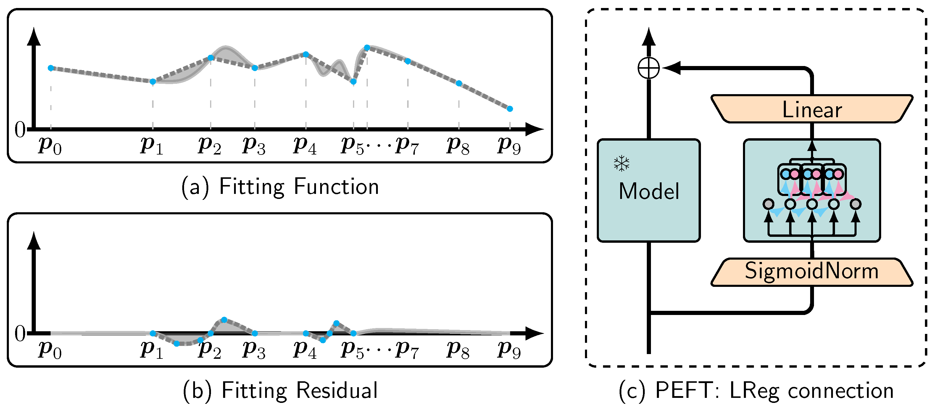
To address this issue, LReg can be incorporated as a module within PEFT methodologies. As shown in Figure 2, consider the target F ( x ) and a pre-trained model f ( x ) . When f ˜ ( x ) is well trained, the residual F ( x ) f ˜ ( x ) remains nearly flat around the value of 0 throughout the input space. This sparsity in the residual’s support set suggests that dimensionality reduction on features could serve as an effective strategy for applying LReg to high-dimensional inputs.
In Figure 1c, we use a SigmoidNorm layer to reduce the input dimensionality:
x Sigmoid ( PCA ( x ) ) .
The built-in Principal Component Analysis (PCA) module can be obtained through standard unsupervised methods or by training. LReg is then applied to learn the residual:
F ( x ) f ˜ ( x ) i c i ψ i ( x ) .
Subsequently, the composed x is converted to { ψ i ( x ) } i by the encoder of LReg. Finally, the linear combination i c i ψ i ( x ) is completed via the Linear layer.
In this scenario, LReg enables the loss function of large pre-trained models to move from local minima. Experiments demonstrate that LReg connection further reduces cross-entropy loss and significantly improves the performance of pre-trained models within a single training epoch (see Section 3.3). This approach effectively fine-tunes the model while preserving computational efficiency.

3. Results

We begin by training LReg from scratch to validate the explicit scaling law in Section 2.6 and identify the limitations of conventional models in fitting multi-frequency data (Section 3.2). The exploration of model fine-tuning for achieving reduced loss function values and enhanced performance is discussed in Section 3.3. For extending the PEFT method to non-transformer-based models via LReg connection, along with comparison results, refer to Section 3.4. Implementation details are provided in Appendix A, while additional applications are discussed in Appendix C.

3.1. Scaling Law and Addressing Regression Challenges

Figure 3 illustrates the performance of the LReg method with varying numbers of model parameters. In these experiments, LReg is trained to approach convergence on fitting the mapping function F : R d R . As shown, the L ( N ) , denoted as test Mean Absolute Error (MAE) loss, is observed to be proportional to the power of the number of model parameters, N 1 / d , and the inverse power of the number of simplices, n t 1 / d , on the triangulation mesh. This observation is in perfect agreement with the derived error-bound formula in Section 2.6.
Notably, the data learned by the model in Figure 3, represented as { ( x , y ) | 1 X U ( 0.02 , 1.0 ) , Y N ( sin 1 x , 0.01 ) } , exhibits multi-frequency characteristics that present significant challenges for conventional neural networks to learn effectively. It is worth noting that although distribution { ( x , y ) | 1 X U ( 0.02 , 1.0 ) , Y N ( sin 1 x , 0.01 ) } and distribution { ( x , y ) | X U ( 1 , 50 ) , Y N ( sin x , 0.01 ) } are equivalent in mathematics, the numerical results of function fitting are completely different. In our open-source GitHub repository, we provide such a demo: for the neural network without LReg connection, the model fits the latter well, but cannot fit the former anyway.
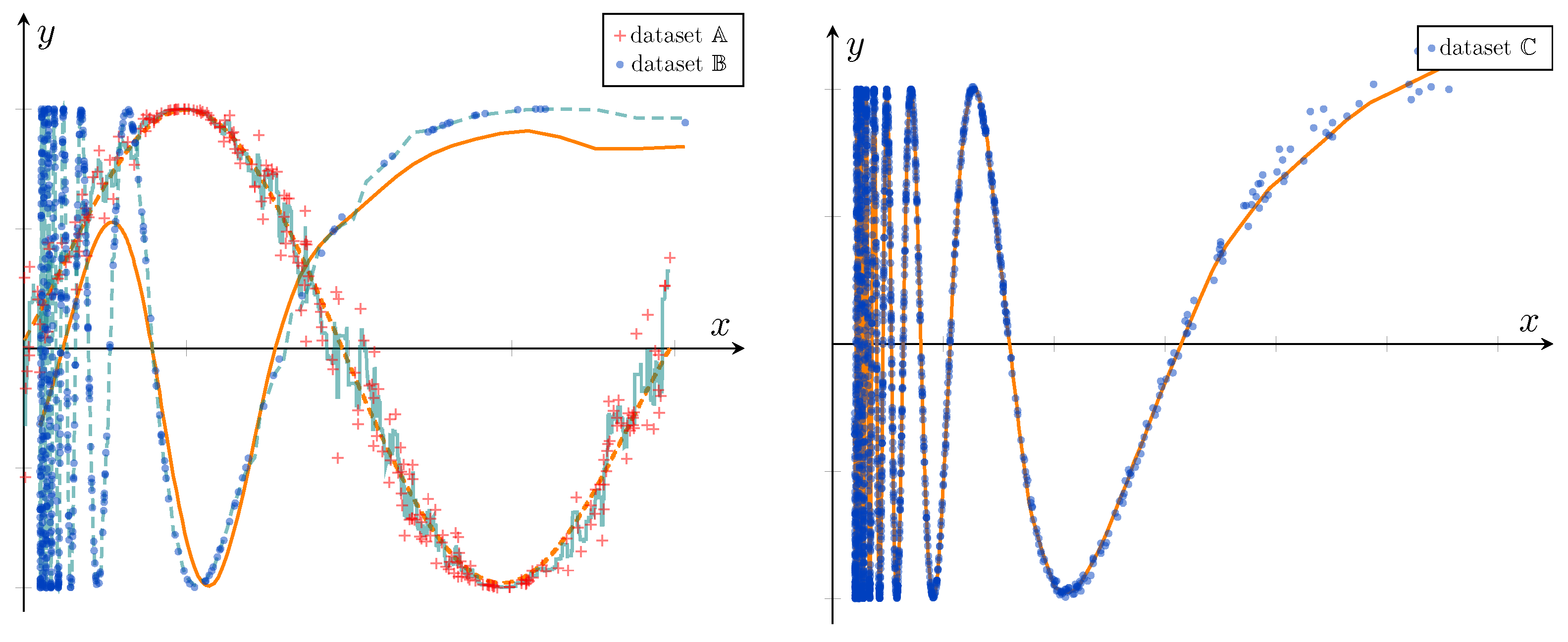
Traditional regressors often struggle with overfitting, while neural networks address this but perform poorly when fitting multi-frequency functions, a phenomenon known as the frequency principle [8]. As shown in Figure 4, Support Vector Regression [9] fits dataset B = { ( x , y ) | 1 X u ( 0.02 , 0.5 ) , y = sin 1 x } but overfits on dataset A , whereas neural networks perform well on A = { ( x , y ) | X u ( 0 , π 4 ) , Y N ( sin 8 x , | cos 8 x | ) } but underfit on B . Neither MLPs, Convolutional Neural Networks (CNNs), nor Transformers can effectively fit sharp transitions in dataset B , often treating these regions as noise to avoid overfitting. Importantly, no existing model can fit the challenging dataset C = { ( x , y ) | 1 X u ( 0.02 , 0.5 ) , Y N ( sin 1 x , 0.5 x 2 ) } .
LReg addresses this gap by combining the strengths of traditional regressors and neural networks. It leverages a multiscale mesh to fit high-frequency regions using fine simplices adaptively. Figure 4 (right) demonstrates the LReg’s unique ability to handle dataset C , a task no other model can achieve. In the next section, we further illustrate its gradual fitting process during training. Comparison experiments in Table 1 show that the LReg consistently achieves high R 2 scores across all test sets, demonstrating its robustness and effectiveness, even in high-noise and multi-frequency scenarios.

3.2. Comparison with Regressors: Training from Scratch

As mentioned earlier, neural networks often struggle to fit multi-frequency datasets effectively. Therefore, our primary focus is comparing the LReg with traditional regressors. To evaluate the effectiveness and generalization of the LReg, we have devised four diverse datasets, each generated from distinct probability distributions:
  • A 1 : Generated from the distribution { ( x , y ) | X U ( π , π ) , Y N ( sin x , 1 5 cos 2 x ) } , with 1000 training examples and 200 test examples. The LReg was trained with a learning rate of 0.1.
  • B 1 : Generated from the distribution { ( x , y ) | 1 X U ( 0.02 , 1.0 ) , Y N ( sin 1 x , 0.01 ) } , with 1000 training examples and 200 test examples. We trained the LReg with a learning rate of 0.9.
  • A 2 : Generated from the distribution { ( x , y ) | X i U ( π , π ) , Y i N ( sin x i , 1 10 cos 2 x i ) ,
    Y = 1 2 ( Y 1 + Y 2 ) } , with 7500 training examples and 1500 test examples. The LReg was trained with a learning rate of 0.1.
  • B 2 : Generated from the distribution { ( x , y ) | 1 x i U ( 0.05 , 0.5 ) , Y i N ( sin 1 x i , 0.01 ) ,
    Y = 1 2 ( Y 1 + Y 2 ) } , with 50,000 training examples and 10,000 test examples. Training utilized a learning rate of 0.9.
Table 1 displays the coefficient of determination ( R 2 ) scores for the LReg and traditional regressors [9,10,11,12,13,14,15,16,17,18] across fitting the four datasets. The LReg consistently achieves high R 2 scores across all test sets, demonstrating the effectiveness of the InterpolationNet on both high-noise and multi-frequency datasets. Furthermore, the minimal gap between training and test set evaluations underscores the robustness of the LReg, indicating its capability of generalization.
We also explore training LReg from scratch on non-regression tasks. Here, we delve into the practical application of LReg for text feature extraction using the AG News dataset [19] for classification tasks. Our experimental findings reveal that LReg can directly extract features from raw text. However, recognizing that tokens are unordered categorical variables, to enhance performance, we add a preprocessing layer that converts each token to a four-dimensional vector, the proportion of the token appearing in four categories.
Our experiment showcases the LReg achieving 90.01% test accuracy after the first epoch, with 90.4% test accuracy reached within just five epochs. It possesses a unique characteristic in text classification tasks: the number of its parameters remains independent of the token count. Compared to word2vec-based networks, our model performs equally well in classification but boasts only 256 model parameters, a significant reduction from the word2vec-based network with more than 6.13 million parameters.

3.3. Improving Pre-Trained Model Performance and Continuously Reducing Loss

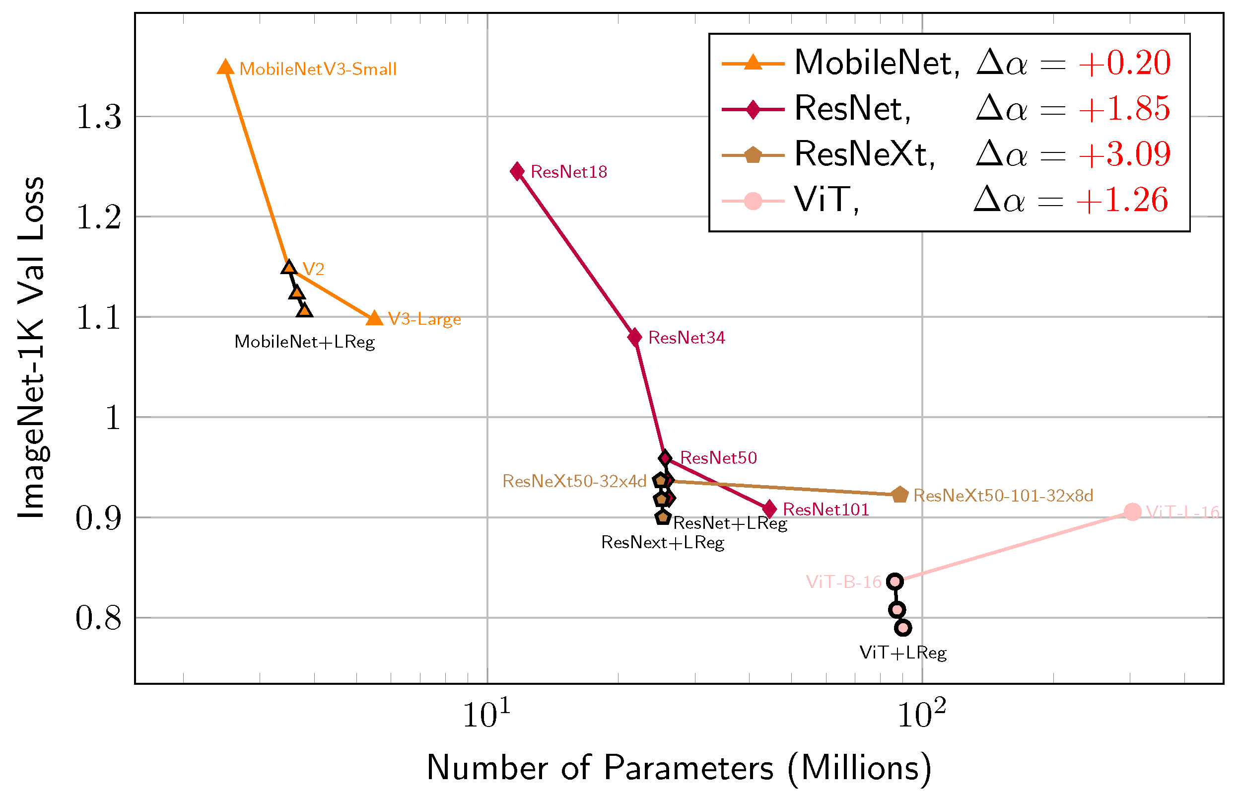
As described in Section 2.7, LReg can serve as a connection to enable the loss function of large pre-trained models to escape local minima (see Figure 5). In this module, the SigmoidNorm layer and linear head contain trainable parameters (see Figure 2c). In this section, we illustrate the effectiveness of LReg connection through ablation studies. To ensure a fair comparison with baseline models, we adopt a stricter experimental setup: the original training recipe of the pre-trained model remains unchanged, the entire pre-trained model is frozen, and no additional training data is used.
This restriction is crucial to ablation studies because the training recipes for pre-trained models often have room for optimization [20]. Changes to batch size, optimizer, weight decay rate, or the order of applying data augmentations could potentially improve the performance of the pre-trained model [21,22]. To avoid such effects, we selected pre-trained models from TorchVision with publicly available training recipes as our baselines. The weights of these pre-trained models closely reproduce the results from the original papers on the ImageNet-1K dataset [23], with recipes available at [24].
Our method offers significant practical value. Unlike model scaling and adaptation approaches, it requires no modifications to the raw training recipe, converges within a single epoch, and is applicable to any model, not limited to the transformer-based architecture. For instance, on 4× A6000 GPUs, it adds fewer than one million parameters to a ResNet-50 model and achieves a 0.2% accuracy gain in just 40 min of training. Due to space constraints, we present some of the comparison results in Table 2.
In Appendix B, we highlight the strong stability of LReg, showing ±0.07% fluctuation in validation accuracy across independent model training (see Appendix B, Table A1). Trainable parameters in our method originate from the SigmoidNorm and linear layer (see Figure 2c). The total number of trainable parameters can be calculated as N = ( C in + 1 ) × d + d × n × C , where N is the number of model parameters, C in is the SigmoidNorm input dimension, d the PCA output dimension, n is the mesh node count (degrees of freedom), and C the total output dimension.
Increasing n and d improves model performance (see Appendix B, Table A2). We also study empirical scaling laws for model performance on cross-entropy loss to demonstrate how our method furthers the loss value of pre-trained models. Ref. [5] proposed an empirical formula where the loss scales as a power-law with model size:
L ( N ) = c N α
where L ( N ) is the cross-entropy loss on the validation dataset, and c and α are constants related to the model type. Figure 5 shows that our method is more effective than simply scaling the model size. Our method increases the α for MobileNet [25] from 0.27 to 0.47, for ResNet [26] from 0.25 to 2.1, for ResNeXt [27] from 0.01 to 3.1, and for ViT [28] from −0.06 to 1.2.

3.4. Transfer Learning via LReg Connection

Through experiments, we identified three key limitations of existing PEFT methods: (1) Dependence on Transfer Learning: Methods like LoRA [29] struggle to outperform pre-trained models on the same or similar datasets, when no domain adaptation is needed. This means they cannot continuously reduce the loss function on the raw training set. Additional training data is often required for these methods to be effective. Therefore, their strength lies mainly in transfer learning scenarios (see Appendix B). (2) Sensitive Training Requirements: PEFT methods require specific training recipes, such as small learning rates. Without these, performance often deteriorates from the first epoch. (3) Task and Architecture Limits: PEFT methods, like LoRA, LoHA [30], and IA3 [31], are restricted to transformer-based architectures.
We compare fine-tuning (FT), BitFit [32], LoRA, and LReg connection on the GLUE dataset [33]; subsequently, we conduct additional experiments on WikiText benchmarks [34] using GPT2 [35] for causal language modeling and Roberta [36] for masked language modeling with a default random seed (42). Pre-trained models of the HuggingFace Transformers library [37] are used. A reduced learning rate (≤10−5) is applied for LoRA to prevent performance degradation in these experiments. As shown in Table 3, our method overcomes the mentioned challenges, performing well even without additional training data. Therefore, it is also versatile for transfer learning.

4. Discussion

It is important to acknowledge the limitations associated with LReg. As described in Section 2.7, the substantial computational cost of extracting features from high-dimensional data restricts its direct application to large-scale datasets. Presently, we address this by incorporating LReg as an adaptation method, but we aim to extract features directly from large-scale data in the future. Additionally, the experiments in Section 3.3 indicate that, although our adaptation method significantly reduces cross-entropy on the ImageNet-1K validation set, the extent of accuracy improvement is relatively modest, warranting further investigation. We did not compare LReg with models such as Support Vector Machine (SVM) known for their robust interpretability, due to fundamentally different underlying principles, and the usual missing experimental results from interpretable models on large datasets. Specifically, we now outline that since our method is plug-and-play and can be integrated into any existing models, and given that large generative models are a prominent trend in AI research, we plan to apply our method to diffusion models and large language models in future studies.

5. Conclusions

In this paper, we reformulate MLPs and introduce a mathematically equivalent framework named LReg. Furthermore, we propose a discrete method, referred to as the MRC loop, which serves as an alternative to traditional continuous optimization techniques, thereby enabling the loss function to reach global minima. For general pre-trained models, we demonstrate that our approach can significantly reduce the loss function value.
From a theoretical perspective, we construct a visual example to elucidate the intrinsic challenge encountered by traditional optimization methods in reducing the loss function from local minima to global minima, and highlight the benefits of discrete parameter updates in addressing this challenge. Furthermore, we analyze the error-bound formula and, for the first time, derive an explicit scaling law, while we empirically validate through regression tasks. From an application perspective, LReg effectively mitigates the core limitation of traditional neural networks in learning multi-frequency data. Additionally, LReg serves as a plug-and-play module, and our analysis of the scaling law shows that it substantially reduces the loss function value of pre-trained models while providing moderate improvement in performance. In contrast to scaling up a model and training it from scratch, our approach is more efficient. Furthermore, LReg broadens the application scope of PEFT methods in transfer learning, without requiring the pre-trained model to be transformer-based.
This work opens new directions for research in model training and establishes a foundation for further advancements in discrete optimization.

Supplementary Materials

The following supporting information can be downloaded at: https://github.com/LizhengMathAi/LReg/tree/main (accessed on 19 October 2025).

Author Contributions

Conceptualization, Z.L. and J.C.; methodology, Z.L.; software, Z.L.; validation, Z.L., J.C., and H.H.G.; formal analysis, Z.L.; investigation, Z.L.; resources, Z.L.; data curation, Z.L.; writing—original draft preparation, Z.L.; writing—review and editing, J.C. and H.H.G.; visualization, Z.L.; supervision, J.C. and H.H.G.; project administration, Z.L. All authors have read and agreed to the published version of the manuscript.

Funding

The work was partially supported by the National Science Foundation Grants CNS-2120350 and III-2311598.

Institutional Review Board Statement

Not applicable.

Informed Consent Statement

Not applicable.

Data Availability Statement

All datasets presented in this paper are openly available: ImageNet [23] (https://www.image-net.org/; GLUE [33] (https://gluebenchmark.com/); WikiText [34] (https://huggingface.co/datasets/Salesforce/wikitext). Accessed on 19 October 2025.

Conflicts of Interest

The authors declare no conflicts of interest.

Abbreviations

The following abbreviations are used in this manuscript:
FEMFinite Element Method
LRegLagrange Regressor
MAEMean Absolute Error
MLPMulti-Layer Perceptron
MRCMesh-Refinement–Coarsening
PCAPrincipal Component Analysis
PEFTParameter-Efficient Fine-Tuning
SVMSupport Vector Machine

Appendix A. Mesh and Lagrange Basis Function

Appendix A.1. Triangulated Mesh

In the context of FEM, elements often serve as the fundamental building blocks of the triangulation mesh, taking the form of simplices created by connecting nodes. For instance, in 1D FEM, simplices are intervals (see Figure 1a); in 2D FEM, triangles with three nodes are commonly used (see Figure A1, right), while 3D FEM often employs tetrahedra with four nodes. This concept is visually depicted in Figure A1 (left), where the mesh consists of eight nodes and seven triangles. This type of mesh is established by specifying the coordinates of discrete nodes and the vertex indices of simplices. Let d represent the dimensions, { p ( i ) } i = 0 n 1 denote the grid nodes, and introduce a matrix P to store the node coordinates:
P i , j = p j ( i ) .
Additionally, utilize a matrix T to store the indices of nodes constituting the simplices within the triangulation. Specifically, access the j-th sorted vertex of the i-th simplex in this mesh as p T i , j , : . Figure A1 (left) illustrating a matrix T takes the following form:
Figure A1. Left—Mesh with eight nodes and seven triangles. Right—Contours of eight Lagrange basis functions, linear variation of ψ i associated with node p ( i ) across all triangles.
Information 16 00921 g0a1
T = 6 0 3 2 7 3 4 7 6 7 3 4 4 3 5 5 1 1 5 7 2 T .
This matrix serves to describe all seven simplices within the mesh, such as the first simplex p ( 6 ) p ( 7 ) p ( 5 ) and the last simplex p ( 4 ) p ( 3 ) p ( 2 ) .
The first-order Lagrange basis studied in this article, denoted as { ψ 0 ( x ) , , ψ n 1 ( x ) } P 1 ( R d ) , consists of piecewise linear polynomials associated with nodes { p ( 0 ) , , p ( n 1 ) } . These functions are defined such that ψ i ( p ( j ) ) = 1 i = j . Figure A1 (right) illustrates this: ψ i ( x ) corresponds to node p ( i ) , exhibiting linear variation across all elements. Its support encompasses the union of all neighboring elements of node p ( i ) (refer to Appendix B for a three-dimensional visualization). For example, supp ( ψ 3 ) = p ( 3 ) p ( 4 ) p ( 7 ) p ( 3 ) p ( 7 ) p ( 1 ) p ( 3 ) p ( 1 ) p ( 2 ) p ( 3 ) p ( 2 ) p ( 4 ) .
Now, we formulate the Lagrange basis from its original definition to establish the foundational architecture of LReg. It is important to highlight that the traditional Lagrange basis involves unbalanced computing of barycentric coordinates, which may not be well-suited for parallel deep learning platforms (see Appendix C for details on the traditional definition of the Lagrange basis). Consequently, in this subsection, we re-derive the Lagrange basis to enhance parallel computing.

Appendix A.2. Lagrange Basis Function

Let n t represent the number of simplices in the multiscale mesh. We introduce the Parameters Tensor S defined as:
S j , : , : = p 0 ( T j , 0 ) p d 1 ( T j , 0 ) 1 p 0 ( T j , d 1 ) p d 1 ( T j , d 1 ) 1 p 0 ( T j , d ) p d 1 ( T j , d ) 1 1 , j = 0 , , n t 1 .
Additionally, we introduce the Node Membership tensor M defined as:
M i , j , k = 1 , if the i - th node matches the k - th vertex of the j - th simplex , 0 , other cases .
By defining:
U j , k ( x ) = τ = 0 d 1 S j , τ , k · x τ + S j , d , k , j = 0 , , n t 1 , k = 0 , , d .
We will demonstrate in Appendix A.3 that the following function qualifies the definition of Lagrange basis:
ψ i ( x ) = j = 0 n t 1 k = 0 d 1 min τ U j , τ ( x ) 0 · M i , j , k · U j , k ( x ) max ( j = 0 n t 1 k = 0 d 1 min τ U j , τ ( x ) 0 · M i , j , k , 1 ) , i = 0 , , n 1 .
So far, we have successfully constructed:
Encoder : R d [ 0 , 1 ] n ,
x ( ψ 0 ( x ) , , ψ n 1 ( x ) ) .
The above basis is in the format of P 1 ( R d ) , which is very useful for low-dimensional regression tasks. In the one-dimensional case, Equation (A6) simplifies to the Lagrange basis P 1 ( R 1 ) :
ψ i ( x ) = min ReLU ( x p i 1 ) p i p i 1 , ReLU ( p i + 1 x ) p i + 1 p i , i = 0 , 1 , , n 1 .
The P 1 ( R 1 ) basis has exceptionally low computational complexity, making its direct sum well-suited for recognition tasks on large-scale datasets. In Section 2.7, we introduce the specific approach in detail. We use the P 1 ( R 1 ) basis to implement an adaptive method for learning a decoupled residual system. This method can enhance the performance of pre-trained models on large datasets.

Appendix A.3. Proof of Lagrange Basis Expression

We will now demonstrate, in three concise steps, that Equation (A6) qualifies as a Lagrange basis function.
Piecewise Linear: Since { U j , 0 , , U j , d } are piecewise linear functions, their linear combination L i is also piecewise linear.
Kronecker Delta: From the definition of U and S , we have the following equation:
x 0 x d 1 1 = U j , 0 ( x ) U j , d ( x ) p 0 ( T j , 0 ) p d 1 ( T j , 0 ) 1 p 0 ( T j , d 1 ) p d 1 ( T j , d 1 ) 1 p 0 ( T j , d ) p d 1 ( T j , d ) 1 .
Decomposing this equation, we obtain x = k = 0 d U j , k ( x ) p ( T j , k ) and k = 0 d U j , k ( x ) = 1 . This implies two important conclusions: U j , k ( p ( T j , k ) ) = 1 k = k and min τ U j , τ ( x ) 0 is true if and only if x belongs to the j-th simplex. Therefore, we have
1 min τ U j , τ ( p ( i ) ) 0 = M i , j , k = U j , k ( p ( i ) ) = 1 , if i = T j , k ; M i , j , k = U j , k ( p ( i ) ) = 0 , if i T j , k .
This proves that ψ i ( p ( j ) ) = 1 i = j .
Global Continuity: Lastly, since ψ i is inherently linear within all simplices and exhibits continuity across all grid nodes, we can conclude that ψ i is globally continuous.

Appendix A.4. Validation of Lagrange Basis Functions’ Mathematical Expression

This section focuses on the mathematical validation of Lagrange basis function expressions to ensure they satisfy our definition in Section 2.4; the Lagrange basis functions are defined as tent-shaped linear functions that take a value of 1 at their specified nodes and 0 at all other nodes. We start with a two-dimensional case and a triangulated mesh. Let triangle △ be defined by nodes { p ( i ) , p ( j ) , p ( k ) } . The following barycentric coordinates { λ , i , λ , j , λ , k } are three first-degree polynomials of x
λ , i ( x ) λ , j ( x ) λ , k ( x ) = p 0 ( i ) p 0 ( j ) p 0 ( k ) p 1 ( i ) p 1 ( j ) p 1 ( k ) 1 1 1 1 x 0 x 1 1 .
Referring to the instance depicted in Figure A1 (left), the mesh consists of eight nodes and seven triangles. Specifically, let { ( j ) = p ( T j , 0 ) p ( T j , 1 ) p ( T j , 2 ) | j = 0 , , 6 } . We will now verify that the following ψ 3 corresponds to the third basis function in this mesh
ψ 3 ( x ) = 1 max ( i { 2 , 3 , 6 , 5 } 1 x ( i ) , 1 ) i { 2 , 3 , 6 , 5 } 1 x ( i ) λ ( i ) , 3 ( x ) .
First, ψ 3 possesses values of Kronecker Delta:
ψ 3 ( x ) = 1 max ( 0 , 1 ) ( 0 · λ ( 2 ) , 3 ( x ) + 0 · λ ( 3 ) , 3 ( x ) + 0 · λ ( 6 ) , 3 ( x ) + 0 · λ ( 5 ) , 3 ( x ) ) = 0 , if x = p ( 0 ) , 1 max ( 2 , 1 ) ( 1 · 0 + 1 · 0 + 0 · λ ( 6 ) , 3 ( x ) + 0 · λ ( 5 ) , 3 ( x ) ) = 0 , if x = p ( 1 ) , 1 max ( 2 , 1 ) ( 0 · λ ( 2 ) , 3 ( x ) + 1 · 0 + 1 · 0 + 0 · λ ( 5 ) , 3 ( x ) ) = 0 , if x = p ( 2 ) , 1 max ( 4 , 0 ) ( 1 · 1 + 1 · 1 + 1 · 1 + 1 · 1 ) = 1 , if x = p ( 3 ) , 1 max ( 2 , 1 ) ( 0 · λ ( 2 ) , 3 ( x ) + 0 · λ ( 3 ) , 3 ( x ) + 1 · 0 + 1 · 0 ) = 0 , if x = p ( 4 ) , 1 max ( 0 , 1 ) ( 0 · λ ( 2 ) , 3 ( x ) + 0 · λ ( 3 ) , 3 ( x ) + 0 · λ ( 6 ) , 3 ( x ) + 0 · λ ( 5 ) , 3 ( x ) ) = 0 , if x = p ( 5 ) , 1 max ( 0 , 1 ) ( 0 · λ ( 2 ) , 3 ( x ) + 0 · λ ( 3 ) , 3 ( x ) + 0 · λ ( 6 ) , 3 ( x ) + 0 · λ ( 5 ) , 3 ( x ) ) = 0 , if x = p ( 6 ) , 1 max ( 2 , 1 ) ( 1 · 0 + 0 · λ ( 3 ) , 3 ( x ) + 0 · λ ( 6 ) , 3 ( x ) + 1 · 0 ) = 0 , if x = p ( 7 ) ,
Then, ψ 3 is a first-degree polynomial in every triangle and supp ψ 3 = inn i { 2 , 3 , 6 , 5 } ( i ) :
ψ 3 ( x ) = 1 max ( 0 , 1 ) ( 0 · λ ( 2 ) , 3 ( x ) + 0 · λ ( 3 ) , 3 ( x ) + 0 · λ ( 6 ) , 3 ( x ) + 0 · λ ( 5 ) , 3 ( x ) ) = 0 , if x inn T 0 , 1 max ( 0 , 1 ) ( 0 · λ ( 2 ) , 3 ( x ) + 0 · λ ( 3 ) , 3 ( x ) + 0 · λ ( 6 ) , 3 ( x ) + 0 · λ ( 5 ) , 3 ( x ) ) = 0 , if x inn T 1 , 1 max ( 1 , 1 ) ( 1 · λ ( 2 ) , 3 ( x ) + 0 · λ ( 3 ) , 3 ( x ) + 0 · λ ( 6 ) , 3 ( x ) + 0 · λ ( 5 ) , 3 ( x ) ) = λ ( 2 ) , 3 ( x ) , if x inn T 2 , 1 max ( 1 , 1 ) ( 0 · λ ( 2 ) , 3 ( x ) + 1 · λ ( 3 ) , 3 ( x ) + 0 · λ ( 6 ) , 3 ( x ) + 0 · λ ( 5 ) , 3 ( x ) ) = λ ( 3 ) , 3 ( x ) , if x inn T 3 , 1 max ( 0 , 1 ) ( 0 · λ ( 2 ) , 3 ( x ) + 0 · λ ( 3 ) , 3 ( x ) + 0 · λ ( 6 ) , 3 ( x ) + 0 · λ ( 5 ) , 3 ( x ) ) = 0 , if x inn T 4 , 1 max ( 1 , 1 ) ( 0 · λ ( 2 ) , 3 ( x ) + 0 · λ ( 3 ) , 3 ( x ) + 0 · λ ( 6 ) , 3 ( x ) + 1 · λ ( 5 ) , 3 ( x ) ) = λ ( 5 ) , 3 ( x ) , if x inn T 5 , 1 max ( 1 , 1 ) ( 0 · λ ( 2 ) , 3 ( x ) + 0 · λ ( 3 ) , 3 ( x ) + 1 · λ ( 6 ) , 3 ( x ) + 0 · λ ( 5 ) , 3 ( x ) ) = λ ( 6 ) , 3 ( x ) , if x inn T 6 ,
Finally, since ψ 3 is continuous in all nodes and first-degree in all triangles, it is globally continuous.

Appendix A.5. Visualization of Lagrangian Basis

In Section 2.4 and Appendix A.2, we introduced first-order Lagrange basis functions, a set of piecewise linear functions defined on a mesh. Each basis function corresponds to a node.
Consider the grid depicted in Figure A2 (left). Taking the inserted fine node p ( 20 ) as an example, it has a total of four neighboring nodes: p ( 5 ) , p ( 0 ) , p ( 7 ) , and p ( 4 ) . By connecting these nodes, we can determine the support of the basis function ψ 20 . In Figure A2 (middle), we present the function graphs of ψ 20 and ψ 7 . It can be observed that these functions exhibit linear variations on each mesh triangle. Taking ψ 20 as an example, its function value at p 20 is 1, and 0 at all other nodes. Similarly, ψ 7 has a function value of 1 at p 7 and 0 at other nodes. In Figure A2 (right), the orange triangles represent the function graph of f ( x ) on the domain p ( 0 ) p ( 7 ) p ( 9 ) , and the green dots represent a subset of the training set { ( x ( i ) , y ( i ) ) } i , where the projections (raw data) fall on p ( 0 ) p ( 7 ) p ( 9 ) . Base on the definition of Lagrange basis function, we have:
f ( x ) | x p ( 0 ) p ( 7 ) p ( 9 ) = i c i ψ i ( x ) | x p ( 0 ) p ( 7 ) p ( 9 ) = c 0 ψ 0 ( x ) + c 7 ψ 7 ( x ) + c 9 ψ 9 ( x ) .
The training process mentioned in Section 2.5 uses the least squares method to adjust coefficients, minimizing the mean gap (MAE) between the green points and the triangular surface.
arg min ( c 0 , c 7 , c 9 ) i | c 0 ψ 0 ( x ( i ) ) + c 7 ψ 0 ( x ( i ) ) + c 9 ψ 0 ( x ( i ) ) y ( i ) | , using model training ; arg min ( c 0 , c 7 , c 9 ) i | c 0 ψ 0 ( x ( i ) ) + c 7 ψ 0 ( x ( i ) ) + c 9 ψ 0 ( x ( i ) ) y ( i ) | 2 , using least squares .
Figure A2. Data visualization. Left—An example of refining a two-dimensional mesh. Middle—The graphs of basis functions ψ 20 and ψ 7 . Right—The graphs of the function f ( x ) and a subset of the training set, adjusting coefficients for minimizing MAE Loss.
Information 16 00921 g0a2

Appendix B. Additional Experiments

We study the robustness of the LReg on the ImageNet-1K validation set with one training epoch. The result is presented in Table A1. All methods follow the raw training recipes to ensure fair comparisons.
Table A1. Classification accuracy on the ImageNet-1K validation set and one epoch training, with all methods adhering to the raw training recipes. We report the changes in the number of model parameters and their ratio of changes and total. For each model, we conducted multiple experiments and show the accuracy as “ mean ± std ( mean baseline ) ”.
Modeldn# ParamsAcc@1 (%)Acc@5 (%)
MobileNet-V23280.298 M (+8.51%) 71.920 ± 0.016   ( + 0.045 ) 90.302 ± 0.021   ( + 0.016 )
ResNet503280.324 M (+1.27%) 76.334 ± 0.054   ( + 0.204 ) 92.976 ± 0.024   ( + 0.114 )
ResNeXt503280.324 M (+1.30%) 77.796 ± 0.063   ( + 0.178 ) 93.653 ± 0.038   ( + 0.178 )
ViT-B-168321.032 M (+1.19%) 81.092 ± 0.012   ( + 0.020 ) 95.316 ± 0.004   ( 0.002 )
Increasing n, d, and training epochs is an effective way to enhance model performance, as shown in Table A2. Unlike the function fitting task, diminishing returns in performance improvements are observed in this case due to the finite cardinality of image and text datasets.
Table A2. ResNet-50 Performance with different n and d. The table explores the impact of varying n (PCA output dimension) and d (degrees of freedom) on the performance of the LagEncoder-based ResNet-50 model. Metrics include the number of additional parameters, top-1 (Acc@1) and top-5 (Acc@5) validation accuracy, and training speed (images per second). The baseline ResNet-50 has 25.6 M parameters, Acc@1: 76.130%, and Acc@5: 92.862%. Results that surpass competing methods are bold.
Coeff (n, d)(4, 4)(4, 8)(4, 16)(4, 32)(8, 4)(8, 8)(8, 16)(8, 32)
# Parameters36,86869,636135,172266,24473,736139,272270,344532,488
Acc@176.22676.22676.24276.22276.23876.25676.26876.276
Acc@592.95292.96092.94892.97292.96492.95492.96692.952
Speed (img/s)405.31411.18390.26418.84382.22394.63409.52404.43
Coeff (n, d) (16, 4)(16, 8)(16, 16)(16, 32)(32, 4)(32, 8)(32, 16)(32, 32)
# Parameters147,472278,544540,6881,064,976294,944557,0881,081,3762,129,952
Acc@176.27276.24476.24876.28476.29876.27276.24876.294
Acc@592.94092.94692.96892.95892.95692.95892.96892.932
Speed (img/s)393.19394.86379.72380.30393.34414.39379.72368.94
To assess the efficiency of LReg, Table A3 compares it with baseline models on both vision and language backbones. The table reports trainable parameters, peak GPU memory, theoretical complexity (GFLOPs), and training speed (images/s and sequence/s). All vision models are evaluated on 224 × 224 images (batch = 32), and language models on 128-token sequences (batch = 2). LReg sharply reduces trainable parameters with minimal change in memory, FLOPs, or throughput.
Table A3. Comparison of computational cost and efficiency between baseline and LReg-enhanced models. For vision networks, memory and throughput are measured during training on a batch of 32 images (224 × 224 pixels). For language models, measurements are taken on a batch of two sequences with a length of 128 tokens. The reported computational complexity (GFLOPs) corresponds to a single 224 × 224 image for vision models and per-token computation for language models. LReg achieves drastic trainable parameter reduction with negligible impact on memory consumption or overall FLOPs.
ModelMethod# Trainable ParametersMemory (MB)GFLOPsThroughput
MobileNet-V2Baseline3.5 M2817.50.60701.51
LReg328,7202823.20.62685.17
ResNet-50Baseline25.6 M3032.44.09440.18
LReg540,6883039.44.10411.50
ResNeXt-50_32x4dBaseline25.0 M4238.24.27334.72
LReg135,1724240.64.27315.33
ViT-B16Baseline86.6 M4744.433.0331.02
LReg67,0764746.233.0316.31
GPT2Baseline124.4 M1428.40.256.98
LReg0.203 M1439.50.269.58
GPT2-MediumBaseline354.8 M3428.80.713.50
LReg0.404 M3445.00.716.66
GPT2-LargeBaseline774.0 M6936.01.5510.05
LReg0.303 M6949.91.5512.37

Appendix C. Additional Applications

Appendix C.1. Solve PDEs

In this section, we utilize the LReg to address the following partial differential equations (PDEs):
Δ u + ( u β ) 2 = ( α cos x sin y 1 ) 2 + 1 , ( x , y ) Ω ; u = β , ( x , y ) Ω ,
where Ω = [ 0 , 1 ] × [ 0 , 1 ] . We construct a dataset that takes ( α , β ) as input data and assigns the corresponding numerical solution of the PDEs as the target output. This dataset comprises 12,000 examples, with α randomly selected from the distribution U ( π / 2 , π / 2 ) and β randomly chosen from the distribution U ( 0 , 2 π ) . We then split the dataset into two parts: 10,000 for training and 2000 for testing. Figure A3 illustrates how well the network predicts the exact solution.
Figure A3. The gap between the exact solution and the model output.
Information 16 00921 g0a3

Appendix C.2. Fitting High-Noise Data

In this section, we conduct the LReg on learning the dataset A = { ( x , y ) | X U ( 4 , 4 ) , Y N ( sin x , 0.2 cos 2 x ) } . A comprises 6000 examples, with 5000 for training and 1000 for testing. Figure A4 shows the training progress.
Figure A4. Blue dots represent the training set, while the orange curve represents the network.
Information 16 00921 g0a4

Appendix C.3. Fitting Multi-Frequency Data

In this section, we conduct the LReg on learning the dataset A = { ( x , y ) | 1 x U ( 0.02 , 0.5 ) , y = sin 1 x } . A comprises 6000 examples, with 5000 for training and 1000 for testing. Figure A5 illustrates the training progress. Remarkably, after just four epochs of training, the neural network outputs closely approximate the target values. By the 32nd epoch’s conclusion, the neural network outputs and target values are nearly indistinguishable.
Figure A5. Blue dots represent the training set, while the orange curve represents the network.
Information 16 00921 g0a5

Appendix C.4. Fit a Vector-Valued Function

In this instance, we utilize the LReg to fit spherical harmonics. Our dataset denoted as A = { ( x , y ) | x = ( θ , ϕ ) , y = ( Real ( Y 4 2 ( θ , ϕ ) ) , Imag ( Y 4 2 ( θ , ϕ ) ) ) , Θ U ( 0 , 2 π ) , Φ U ( 0 , π ) } comprises 48,000 examples, with 40,000 allocated for training and an additional 8000 for testing. Figure A6 shows the training progress.
Figure A6. In each block, the left panel represents the real part of our model output, while the right panel represents the imaginary part of the model output.
Information 16 00921 g0a6

References

  1. Saxe, A.M.; McClelland, J.L.; Ganguli, S. Exact solutions to the nonlinear dynamics of learning in deep linear neural networks. arXiv 2013, arXiv:1312.6120. [Google Scholar]
  2. Dauphin, Y.N.; Pascanu, R.; Gulcehre, C.; Cho, K.; Ganguli, S.; Bengio, Y. Identifying and attacking the saddle point problem in high-dimensional non-convex optimization. arXiv 2014, arXiv:1406.2572. [Google Scholar]
  3. Goodfellow, I.J.; Vinyals, O.; Saxe, A.M. Qualitatively characterizing neural network optimization problems. arXiv 2014, arXiv:1412.6544. [Google Scholar]
  4. Choromanska, A.; Henaff, M.; Mathieu, M.; Arous, G.B.; LeCun, Y. The loss surfaces of multilayer networks. In Proceedings of the Artificial Intelligence and Statistics, PMLR, San Diego, CA, USA, 9–12 May 2015; pp. 192–204. [Google Scholar]
  5. Kaplan, J.; McCandlish, S.; Henighan, T.; Brown, T.B.; Chess, B.; Child, R.; Gray, S.; Radford, A.; Wu, J.; Amodei, D. Scaling laws for neural language models. arXiv 2020, arXiv:2001.08361. [Google Scholar] [CrossRef]
  6. Henighan, T.; Kaplan, J.; Katz, M.; Chen, M.; Hesse, C.; Jackson, J.; Jun, H.; Brown, T.B.; Dhariwal, P.; Gray, S.; et al. Scaling laws for autoregressive generative modeling. arXiv 2020, arXiv:2010.14701. [Google Scholar] [CrossRef]
  7. Zienkiewicz, O.C.; Taylor, R.L.; Nithiarasu, P.; Zhu, J. The Finite Element Method; Elsevier: Amsterdam, The Netherlands, 1977; Volume 3. [Google Scholar]
  8. Xu, Z.Q.J.; Zhang, Y.; Xiao, Y. Training behavior of deep neural network in frequency domain. In Proceedings of the International Conference on Neural Information Processing, Sydney, NSW, Australia, 12–15 December 2019; Springer: Cham, Switzerland, 2019; pp. 264–274. [Google Scholar]
  9. Platt, J. Probabilistic outputs for support vector machines and comparisons to regularized likelihood methods. Adv. Large Margin Classif. 1999, 10, 61–74. [Google Scholar]
  10. Thiel, H. A rank-invariant method of linear and polynomial regression analysis. I, II, III. Nederl. Akad. Wetensch. 1950, 53, 386–392. [Google Scholar]
  11. Cantzler, H. Random Sample Consensus (Ransac); Institute for Perception, Action and Behaviour, Division of Informatics University of Edinburgh: Edinburgh, Scotland, 1981. [Google Scholar]
  12. Zhang, T. Solving large scale linear prediction problems using stochastic gradient descent algorithms. In Proceedings of the Twenty-First International Conference on Machine Learning, Banff, AB, Canada, 4–8 July 2004; p. 116. [Google Scholar]
  13. Hilt, D.E.; Seegrist, D.W. Ridge, a Computer Program for Calculating Ridge Regression Estimates; Department of Agriculture, Forest Service, Northeastern Forest Experiment: Washington, DC, USA, 1977; Volume 236.
  14. Stone, M. Cross-validatory choice and assessment of statistical predictions. J. R. Stat. Soc. Ser. B (Methodol.) 1974, 36, 111–133. [Google Scholar] [CrossRef]
  15. Jain, P.; Kakade, S.M.; Kidambi, R.; Netrapalli, P.; Sidford, A. Accelerating stochastic gradient descent for least squares regression. In Proceedings of the Conference on Learning Theory, PMLR, Stockholm, Sweden, 6–9 July 2018; pp. 545–604. [Google Scholar]
  16. Murphy, K.P. Machine Learning: A Probabilistic Perspective; MIT Press: Cambridge, MA, USA, 2012. [Google Scholar]
  17. Friedman, J.H. Greedy function approximation: A gradient boosting machine. Ann. Stat. 2001, 29, 1189–1232. [Google Scholar] [CrossRef]
  18. Breiman, L. Random forests. Mach. Learn. 2001, 45, 5–32. [Google Scholar] [CrossRef]
  19. Zhang, X.; Zhao, J.; LeCun, Y. Character-level convolutional networks for text classification. arXiv 2015, arXiv:1509.01626. [Google Scholar]
  20. Wightman, R.; Touvron, H.; Jégou, H. Resnet strikes back: An improved training procedure in timm. arXiv 2021, arXiv:2110.00476. [Google Scholar] [CrossRef]
  21. Touvron, H.; Vedaldi, A.; Douze, M.; Jégou, H. Fixing the train-test resolution discrepancy. In Proceedings of the Advances in Neural Information Processing Systems 32 (NeurIPS 2019), Vancouver, BC, Canada, 8–14 December 2019. [Google Scholar]
  22. Touvron, H.; Cord, M.; Douze, M.; Massa, F.; Sablayrolles, A.; Jégou, H. Training data-efficient image transformers & distillation through attention. In Proceedings of the International Conference on Machine Learning, PMLR, Virtual, 18–24 July 2021; pp. 10347–10357. [Google Scholar]
  23. Russakovsky, O.; Deng, J.; Su, H.; Krause, J.; Satheesh, S.; Ma, S.; Huang, Z.; Karpathy, A.; Khosla, A.; Bernstein, M.; et al. Imagenet large scale visual recognition challenge. Int. J. Comput. Vis. 2015, 115, 211–252. [Google Scholar] [CrossRef]
  24. TorchVision Contributors. TorchVision Models. 2024. Available online: https://pytorch.org/vision/master/models.html (accessed on 9 August 2024).
  25. Howard, A.G.; Zhu, M.; Chen, B.; Kalenichenko, D.; Wang, W.; Weyand, T.; Andreetto, M.; Adam, H. Mobilenets: Efficient convolutional neural networks for mobile vision applications. arXiv 2017, arXiv:1704.04861. [Google Scholar] [CrossRef]
  26. He, K.; Zhang, X.; Ren, S.; Sun, J. Deep residual learning for image recognition. In Proceedings of the IEEE Conference on Computer Vision and Pattern Recognition, Las Vegas, NV, USA, 27–30 June 2016; pp. 770–778. [Google Scholar]
  27. Xie, S.; Girshick, R.; Dollár, P.; Tu, Z.; He, K. Aggregated residual transformations for deep neural networks. In Proceedings of the IEEE Conference on Computer Vision and Pattern Recognition, Honolulu, HI, USA, 21–26 July 2017; pp. 1492–1500. [Google Scholar]
  28. Dosovitskiy, A.; Beyer, L.; Kolesnikov, A.; Weissenborn, D.; Zhai, X.; Unterthiner, T.; Dehghani, M.; Minderer, M.; Heigold, G.; Gelly, S.; et al. An image is worth 16x16 words: Transformers for image recognition at scale. arXiv 2020, arXiv:2010.11929. [Google Scholar]
  29. Hu, E.J.; Shen, Y.; Wallis, P.; Allen-Zhu, Z.; Li, Y.; Wang, S.; Wang, L.; Chen, W. Lora: Low-rank adaptation of large language models. arXiv 2021, arXiv:2106.09685. [Google Scholar]
  30. Hyeon-Woo, N.; Ye-Bin, M.; Oh, T.H. Fedpara: Low-rank hadamard product for communication-efficient federated learning. arXiv 2021, arXiv:2108.06098. [Google Scholar]
  31. Liu, H.; Tam, D.; Muqeeth, M.; Mohta, J.; Huang, T.; Bansal, M.; Raffel, C.A. Few-shot parameter-efficient fine-tuning is better and cheaper than in-context learning. Adv. Neural Inf. Process. Syst. 2022, 35, 1950–1965. [Google Scholar]
  32. Zaken, E.B.; Ravfogel, S.; Goldberg, Y. Bitfit: Simple parameter-efficient fine-tuning for transformer-based masked language-models. arXiv 2021, arXiv:2106.10199. [Google Scholar]
  33. Wang, A. Glue: A multi-task benchmark and analysis platform for natural language understanding. arXiv 2018, arXiv:1804.07461. [Google Scholar]
  34. Merity, S.; Xiong, C.; Bradbury, J.; Socher, R. Pointer sentinel mixture models. arXiv 2016, arXiv:1609.07843. [Google Scholar] [CrossRef]
  35. Radford, A.; Wu, J.; Child, R.; Luan, D.; Amodei, D.; Sutskever, I. Language models are unsupervised multitask learners. OpenAI Blog 2019, 1, 9. [Google Scholar]
  36. Liu, Y. Roberta: A robustly optimized bert pretraining approach. arXiv 2019, arXiv:1907.11692. [Google Scholar]
  37. Wolf, T.; Debut, L.; Sanh, V.; Chaumond, J.; Delangue, C.; Moi, A.; Cistac, P.; Rault, T.; Louf, R.; Funtowicz, M.; et al. Transformers: State-of-the-art natural language processing. In Proceedings of the 2020 Conference on Empirical Methods in Natural Language Processing: System Demonstrations, Online, 16–20 November 2020; pp. 38–45. [Google Scholar]
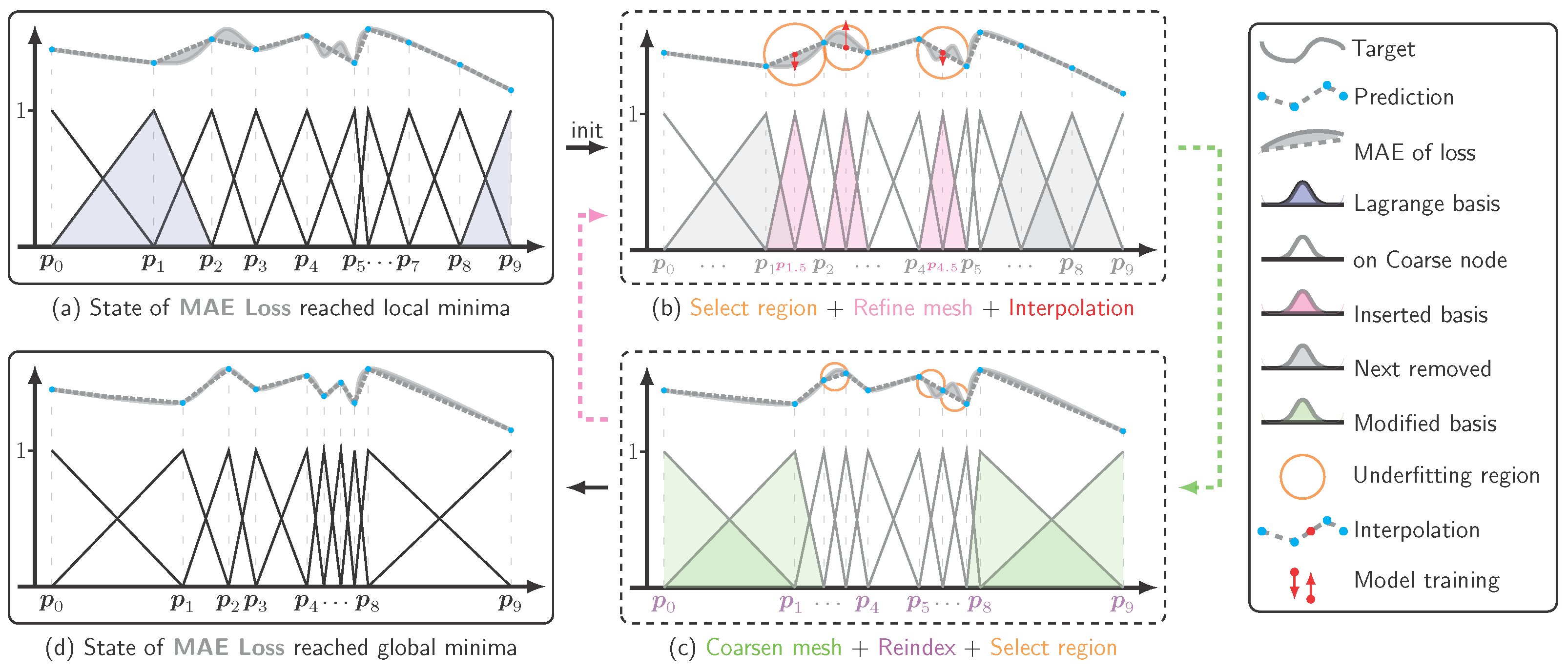
Figure 1. Transition a loss function from a local minimum to a global minimum. (a) Local Minimum: The MLP, based on linear layers and ReLU activations, is represented as a segmented line. Slight adjustments to this segmented line increase the area of shaded region, which represents the MAE; (b) Refinement: Detect underfitting regions of the MLP and insert midpoints to reduce the MAE; (c) Coarsening: Remove nodes with minimal impact on the MAE, decreasing the number of model parameters back to its original count. Scale up the corresponding Lagrange basis and return to Step b; (d) Global Minimum: The shaded area representing the MAE is minimized.
Information 16 00921 g001
Figure 2. Fitting function vs. fitting residual. (a) Fitting a function F ( x ) by training a model from scratch; (b) fitting the residual F ( x ) f ˜ ( x ) using the pre-trained model f ˜ ( x ) from (a); (c) LReg is applied as a shortcut connection to fit the residual F ( x ) f ˜ ( x ) , where the pre-trained model f ˜ ( x ) is kept frozen.
Information 16 00921 g002
Figure 3. Left—Results of 32 experiments fitting the one-dimensional function y = sin 1 x , with each gray point representing an experiment. The figure shows the relationship between n t 1 and test MAE loss. Right—Results of 32 experiments fitting the two-dimensional function y = i = 1 2 sin x i 2 π , with each gray point representing an experiment. The figure shows the relationship between n t 1 / 2 and test loss.
Information 16 00921 g003
Figure 4. Left—Performance of traditional regressors and neural networks on high-noise dataset A and multi-frequency dataset B . The dashed teal curve shows that traditional regressors (e.g., Support Vector Regression) succeed on B but overfit A (solid teal curve). In contrast, neural networks (e.g., MLP) fit A well (dashed orange curve) but underfit B (solid orange curve). Right—The LReg demonstrates exceptional adaptability, successfully learning dataset C , which incorporates both high noise and multi-frequency features.
Information 16 00921 g004
Figure 5. LReg connection greatly reduces the loss function value. Colored lines represent pre-trained models across varying scales, while black lines represent our method, which significantly decreases cross-entropy loss on the ImageNet-1 validation set and outperforms model scaling with negligible changes to the model size.
Information 16 00921 g005
Table 1. A comprehensive comparison between the LReg and traditional regressors. The left half of each paired column displays the training R 2 score, while the right half showcases the corresponding test R 2 score.
Method A 1 B 1 A 2 B 2
OLS Linear0.0370.0420.9630.9510.0850.0920.9840.984
Theil-Sen−44.7−54.40.9580.946−0.41−3.810.9820.982
RANSAC−1.21−1.430.9630.951−27.0−27.10.9830.983
Huber0.0360.0410.9620.9490.0850.0920.9840.984
Ridge0.0310.0380.9630.9510.0550.0610.9840.984
RidgeCV0.0370.0420.9630.9510.0850.0920.9840.984
SGD0.0090.010.9620.950.0050.0040.9830.983
KRR0.00360.040.970.9620.0560.0510.9930.992
SVR0.110.1010.970.9620.290.3080.9920.992
Voting0.8520.8520.9420.9170.8690.8680.9510.946
LReg1.01.00.9710.9630.9990.9990.9920.992
Table 2. Comparison of LReg with baseline models across different architectures. LReg improves top-1 accuracy while introducing only a negligible increase in trainable parameters. It also achieves either comparable or superior training efficiency by converging within five training epochs, thereby significantly reducing training time compared to full model training. Unlike baseline models that require days of training, LReg enhances performance within an hour. These results demonstrate the effectiveness of LReg as a general, parameter-efficient fine-tuning method for large-scale models, without being limited to transformer-based architectures. Results that surpass competing methods are bold. * indicates numbers published in prior works.
ModelMethod# Trainable
Parameters
Acc@1Acc@5Speed
(img/s)
Training
Time (Total)
MobileNet-V2Baseline *3.5 M71.87890.286701.5116 h 37 m
LReg328,72071.93490.268685.1732 m 12 s
ResNet-50Baseline *25.6 M76.13092.862440.182 d 1 h 15 m
LReg540,68876.27492.932411.5040 m 42 s
ResNeXt-50_32x4dBaseline *25.0 M77.61893.698334.723 d 1 h 32 m
LReg135,17277.65093.672315.3351 m 9 s
ViT-B16Baseline *86.6 M81.07295.318331.023 d 3 h 26 m
LReg67,07681.08295.316316.3156 m 54 s
Table 3. GPT2 and RoBERTa with Different Adaptation Methods on the GLUE dataset and WikiText Benchmark. We report the overall (both matched and mismatched) accuracy for MNLI and the accuracy for other tasks. For each model, we conducted multiple experiments and show the accuracy as “ mean ± std ”. For a fair comparison, we adjusted the number of parameters of our method to be similar to those of LoRA. * indicates numbers published in prior works. We also report the number of trainable parameters, perplexity (PPL, with lower values being preferable), and training throughput (measured in sequences per second) for language modeling tasks. Results that surpass competing methods are bold.
MNLISST-2MRPCQNLIQQPRTE
Method # Params Accuracy # Params Accuracy # Params Accuracy # Params Accuracy # Params Accuracy # Params Accuracy
FT *125 M87.6125 M94.8125 M90.2125 M92.8125 M91.9125 M78.7
BitFit *0.1 M84.70.1 M93.70.1 M92.70.1 M91.80.1 M84.00.1 M81.5
LoRA *0.295 M87.5±0.30.295 M 95.1 ± 0.2 0.295 M 89.7 ± 0.7 0.295 M 93.3 ± 0.3 0.295 M 90.8 ± 0.1 0.295 M 86.6 ± 0.7
LReg0.259 M 87.9 ± 0.5 0.259 M 95.3 ± 0.6 0.259 M 90.5 ± 0.4 0.259 M 93.5 ± 0.2 0.259 M 89.7 ± 0.4 0.259 M 83.5 ± 0.3
GPT2GPT2-MediumGPT2-LargeRoberta-Base
Method# ParamsPPLSeq/s# ParamsPPLSeq/s# ParamsPPLSeq/s# ParamsPPLSeq/s
FT124.4 M21.42346.98354.8 M15.89003.50774.0 M13.84681.58124.7 M3.641510.05
LoRA0.295 M21.418812.900.393 M15.88736.290.737 M13.84861.670.295 M3.64259.85
LReg0.203 M21.34019.580.404 M15.86746.660.607 M13.84432.520.303 M3.641412.37
Disclaimer/Publisher’s Note: The statements, opinions and data contained in all publications are solely those of the individual author(s) and contributor(s) and not of MDPI and/or the editor(s). MDPI and/or the editor(s) disclaim responsibility for any injury to people or property resulting from any ideas, methods, instructions or products referred to in the content.