From Subset-Sum to Decoding: Improved Classical and Quantum Algorithms via Ternary Representation Technique

Abstract

The subset-sum problem, a foundational NP-hard problem in theoretical computer science, serves as a critical building block for cryptographic constructions. This work introduces novel classical and quantum heuristic algorithms for the random subset-sum problem at density $d=1$, where exactly one solution is expected. Classically, we propose the first algorithm based on a ternary tree representation structure, inspired by recent advances in lattice-based cryptanalysis. Through numerical optimization, our method achieves a time complexity of $\widetilde{𝒪}\left(2^{0.2400n}\right)$ and space complexity of $\widetilde{𝒪}\left(2^{0.2221n}\right)$, improving upon the previous best classical heuristic result of $\widetilde{𝒪}\left(2^{0.2830n}\right)$. In the quantum setting, we develop a corresponding algorithm by integrating the classical ternary representation technique with a quantum walk search framework. The optimized quantum algorithm attains a time and space complexity of $\widetilde{𝒪}\left(2^{0.1843n}\right)$, surpassing the prior state-of-the-art quantum heuristic of $\widetilde{𝒪}\left(2^{0.2182n}\right)$. Furthermore, we apply our algorithms to information set decoding in code-based cryptography. For half-distance decoding, our classical algorithm improves the time complexity to $\widetilde{𝒪}\left(2^{0.0453n}\right)$, surpassing the previous best of $\widetilde{𝒪}\left(2^{0.0465n}\right)$. For full-distance decoding, we achieve a quantum complexity of $\widetilde{𝒪}\left(2^{0.058326n}\right)$, advancing beyond the prior best quantum result of $\widetilde{𝒪}\left(2^{0.058696n}\right)$. These findings demonstrate the broad applicability and efficiency of our ternary representation technique across both classical and quantum computational models.

1. Introduction

The subset-sum problem, also referred to as the knapsack problem, stands as one of the most fundamental and well-known NP-hard problems in theoretical computer science [1]. Owing to its computational intractability, it has been widely employed in the construction of cryptographic systems [2,3,4,5]. Moreover, this problem underpins several cryptographic schemes targeting post-quantum security (see, e.g., ref. [6]) and acts as a key component in certain quantum hidden shift algorithms [7]. These, in turn, are applied in quantum cryptanalysis of isogeny-based protocols [8] and symmetric cryptographic constructions [9].

An instance of the problem is specified by n integers $(a_1,a_2,\dots ,a_n)\in {\left({\mathbb{Z}}_{2^n}\right)}^n$ and a target integer $s\in {\mathbb{Z}}_{2^n}$. There are two common formulations: the decision version, which is to verify the existence of a subset of $\{a_1,a_2,\dots ,a_n\}$ summing to s, and the computational version, which requires finding such a subset. The decision subset-sum problem is NP-complete. Moreover, given oracle access to the decision problem, a solution to the computational version can be recovered with n queries. When the instance is uniformly random, the problem is termed the random subset-sum problem (RSSP).

The density of an instance is defined as $d=n/{log}_2\left({max}_i{a}_i\right)$. For a random instance $\mathbf{a}$, the density is closely related to the expected number of solutions. In the high-density regime where $d=\mathrm{\Omega }\left(1/logn\right)$, dynamic programming offers an efficient solution [10]. In the low-density setting, Brickell [11] and Lagarias and Odlyzko [12] demonstrated that given oracle access to the shortest vector problem in lattices [13], RSSP can be solved efficiently for densities $d<0.64$. Coster et al. [14] and Joux and Stern [15] further raised this bound to $d<0.94$. For knapsack instances with density approaching 1, the best known algorithms exhibit exponential-time complexity, rendering them computationally intractable; this inherent difficulty is the reason for their designation as “hard” knapsacks.

This work addresses the random subset-sum problem at density $d=1$, where exactly one solution is expected to exist. Horowitz and Sahni’s Meet-in-the-Middle approach [16] reduces the time and space complexity from $𝒪\left(2^n\right)$ to $𝒪\left(2^{n/2}\right)$, avoiding the need for an exhaustive search over all $2^n$ subsets. The idea of the method is to find a collision between two lists of partial sums, each comprising $2^{n/2}$ elements. Schroeppel and Shamir [17] refined this approach with a strategy based on merging four lists, which lowered the space complexity to $𝒪\left(2^{n/4}\right)$.

A significant heuristic algorithm was proposed by Howgrave-Graham and Joux (HGJ) [18] at EUROCRYPT 2010, solving the RSSP with a time complexity of $\widetilde{𝒪}\left(2^{0.337n}\right)$ and a space complexity of $\widetilde{𝒪}\left(2^{0.311n}\right)$, thus breaking the long-standing $2^{n/2}$ barrier. Their key innovation was the use of the representation technique, in which the solution is expressed ambiguously as a sum of vectors in ${\{0,1\}}^n$. This expands the size of the search space and enables the merging of more lists under arbitrary constraints, leading to improved time efficiency. The time and space complexity is derived via numerical optimization, under the standard heuristic assumption that the individual elements obtained in the merging steps are well-distributed. Becker, Coron, and Joux (BCJ) [19] subsequently reduced the time and space complexity to $\widetilde{𝒪}\left(2^{0.291n}\right)$ by introducing representations using vectors from ${\{-1,0,1\}}^n$. Later, Bonnetain, Bricout, Schrottenloher, and Shen (BBSS) [20] further reduced the time and space complexity to $\widetilde{𝒪}\left(2^{0.283n}\right)$ by relaxing BCJ constraints and permitting representations in ${\{-1,0,1,2\}}^n$. Not only has the representation technique been employed as a tool for the subset-sum problem but it has also been successfully applied to the syndrome decoding problem [21,22,23,24] and the learn-with-errors (LWE) problem [25,26,27,28,29].

Quantum algorithms for the subset-sum problem have also attracted significant attention. The first quantum speedup was achieved by Bernstein, Jeffery, Lange, and Meurer (BJLM) [30], who proposed an algorithm leveraging the HGJ technique, achieving a time and space complexity of $\widetilde{𝒪}\left(2^{0.241n}\right)$. Helm and May (HM) [31] subsequently developed a quantum variant of the BCJ algorithm that obtains a time and space complexity of $\widetilde{𝒪}\left(2^{0.226n}\right)$. Later, Bonnetain et al. [20] introduced a quantum algorithm based on their classical algorithm, attaining the time and space complexity of $\widetilde{𝒪}\left(2^{0.218n}\right)$ under the same classical heuristic assumptions.

1.1. Our Contribution

In this work, we introduce a new heuristic algorithm for the subset-sum problem based on a ternary representation technique. The algorithm is further accelerated within a quantum walk search framework, leading to a novel quantum approach.

Representation-based algorithms for the subset-sum problem typically enhance efficiency by increasing the number of representations. These methods inherently exhibit a search tree structure. By recursively constructing parent lists from child lists until reaching a root list that is expected to contain a solution, such algorithms effectively navigate the problem space. To date, all known classical heuristic algorithms employ a binary tree structure. Notably, Lee et al. [29] demonstrated in the context of ternary LWE cryptanalysis that ternary trees significantly increase the number of representations compared to binary trees. Inspired by their idea, we propose the first classical heuristic algorithm for the random subset-sum problem (RSSP) based on a ternary tree structure. Through numerical optimization, we show that our algorithm achieves a time complexity of $\widetilde{𝒪}\left(2^{0.2400n}\right)$ and a space complexity of $\widetilde{𝒪}\left(2^{0.2221n}\right)$, which, to the best of our knowledge, represents the current state of the art among classical heuristic algorithms.

In the quantum setting, we develop a novel quantum algorithm by integrating the proposed classical heuristic with a quantum walk over the Johnson graph, under the MNRS (Magniez–Nayak–Roland–Santha) framework [32]. This quantum algorithm retains the same heuristic foundation as its classical counterpart. After numerical optimization, we demonstrate that it achieves a time and space complexity of $\widetilde{𝒪}\left(2^{0.1843n}\right)$, establishing the best-known quantum heuristic performance for RSSP.

A summary of these complexity results is provided in

Table 1. Comparison of complexity exponent of subset-sum algorithms: classical and quantum approaches.

	Algorithm	Time Complexity	Space Complexity
Classical	HGJ	$0.337$	$0.311$
	BCJ	$0.291$	$0.291$
	BBSS	$0.2830$	$0.2830$
	Ours	$\mathbf{0}.\mathbf{2400}$	$\mathbf{0}.\mathbf{2221}$
Quantum	BJLM	$0.241$	$0.241$
	HM	$0.226$	$0.226$
	BBSS	$0.2182$	$0.2182$
	Ours	$\mathbf{0}.\mathbf{1843}$	$\mathbf{0}.\mathbf{1843}$

Note: Bold values highlight the best (lowest) complexity exponents in each category.

.

Furthermore, we apply both our classical and quantum algorithms to the decoding problem. Code-based cryptography, which relies on the hardness of decoding random linear codes, is a major candidate for post-quantum cryptography (PQC). Three of the four encryption schemes chosen in the fourth round of the NIST PQC standardization project [33] are code-based schemes, namely, Classic McEliece [34], BIKE [35], and HQC [36]. Among these, only HQC was ultimately selected for standardization. This prominence underscores the importance of rigorous security analysis for such systems.

Our decoding algorithms operate within the framework of information set decoding (ISD). The first classical ISD algorithm was introduced by Prange in 1962 [37]. Subsequent improvements were made by Stern [38] and Finiasz and Sendrier [39]. Later, further advancements were achieved through the use of representation techniques by May, Meurer, and Thomae (MMT) [21] as well as by Becker, Joux, May, and Meurer (BJMM) [22]. These were later enhanced by combining representation techniques with nearest neighbor searches, as proposed by May and Ozerov (MO) [40] and Both and May (BM) [41]. Currently, the Both–May algorithm [41] achieves the optimal time complexity among classical algorithms. Recent work has also explored time–memory trade-offs [42,43,44].

By applying our subset-sum algorithm to half-distance decoding, we improve upon the best-known ISD algorithm by Both–May, reducing the time complexity from $\widetilde{𝒪}\left(2^{0.0465n}\right)$ to $\widetilde{𝒪}\left(2^{0.0453n}\right)$. For full-distance decoding, our algorithm achieves a time complexity of $\widetilde{𝒪}\left(2^{0.0973n}\right)$, improving upon the previous $\widetilde{𝒪}\left(2^{0.1020n}\right)$ [22], which relied solely on representation techniques. Although this result does not surpass the state-of-the-art complexity of $\widetilde{𝒪}\left(2^{0.0885n}\right)$ attained by BM [41]—which combines both representation and nearest neighbor techniques—we anticipate that integrating our ternary representation approach with nearest neighbor search could lead to further improvements.

Quantum variants of ISD have been less extensively explored: Bernstein [45] analyzed a quantum version of Prange’s algorithm, and Kachigar and Tillich (KT) [23] later proposed several quantum-walk-based ISD algorithms, which currently represent the fastest known quantum ISD algorithms. Kirshanova [24] provided an alternative perspective on the quantum-walk-based KT algorithms and developed a quantum version of the MO algorithm. In this work, we propose a novel quantum ISD algorithm that outperforms the state-of-the-art algorithm by Kachigar and Tillich. A summary of the complexity results for ISD is provided in

Table 2. Comparison of time complexity exponent of ISD: classical and quantum approaches.

	Algorithm	Full Distance	Half Distance
Classical	Prange	$0.1206$	$0.0576$
	MMT	$0.1116$	$0.0537$
	BJMM	$0.1019$	$0.0494$
	MO	$0.0953$	$0.0473$
	BM	$\mathbf{0}.\mathbf{0885}$	$0.0465$
	Ours	$0.0973$	$\mathbf{0}.\mathbf{0453}$
Quantum	Bernstein	$0.060350$	$--$
	KT	$0.058696$	$--$
	Kirshanova	$0.059450$	$--$
	Ours	$\mathbf{0}.\mathbf{058326}$	$--$

Note: Bold values highlight the best (lowest) complexity exponents in each category.

.

1.2. Organization

The remainder of this paper is structured as follows. Section 2 introduces essential preliminary concepts required for our subsequent analysis and illustrates representation techniques, in particular using the HGJ algorithm as an example. In Section 3, we first present our new classical heuristic subset-sum algorithm, detailing its procedure, explaining its correctness, and analyzing its complexity. Then, through rigorous mathematical derivation, we provide a provable probabilistic algorithm that does not rely on heuristics. In Section 4, we turn to quantum algorithms, explaining in detail how the newly proposed classical algorithm is combined with a quantum walk and subsequently analyzing the complexity of the resulting algorithm. In Section 5, we apply our new classical and quantum algorithms to the decoding problem, demonstrating how they can be incorporated into the information set decoding framework. Specifically, the quantum algorithm employs a nested structure combining Grover search and quantum walks. Finally, in Section 6, we conclude with a summary of our new results.

2. Preliminaries

This section introduces the foundational definitions and standard notations for the subset-sum problem, followed by an overview of representation techniques, illustrated through the HGJ algorithm.

2.1. Notations and Conventions

Definition 1

(Distributions of knapsacks). A knapsack (or subknapsack) is a vector $\mathbf{e}\in D^n$ where $D=\{-1,0,1\}$ is the digit set. We denote by $D^n[\alpha ,\beta ]$ the set of vectors $\mathbf{e}$ containing exactly $\alpha n$ entries equal to $-1$, $(\alpha +\beta )n$ entries equal to 1, and $(1-2\alpha -\beta )n$ entries equal to 0.

Definition 2

(Random subset-sum instance). Let $\mathbf{a}\in {\left({\mathbb{Z}}_N\right)}^n$ be chosen uniformly at random, where $N\simeq 2^n$. For $\beta \in [0,1]$, sample a vector $\mathbf{e}$ uniformly from $D^n\left[0,\beta \right]$, and define $s\equiv \langle \mathbf{a},\mathbf{e}\rangle modN$. Then the pair $(\mathbf{a},s)\in {\left({\mathbb{Z}}_N\right)}^{n+1}$ is termed a random subset-sum instance. Any vector ${\mathbf{e}}^{\prime }\in {\{0,1\}}^n$ satisfying $\langle \mathbf{a},{\mathbf{e}}^{\prime }\rangle \equiv smodN$ is called a solution to the instance.

It is well established that the parameter choice $\beta =1/2$ represents the most computationally challenging scenario, as the vector $\mathbf{e}$ contains an equal proportion of zeros and ones, thereby maximizing combinatorial complexity. Consequently, this paper concentrates exclusively on this specific case.

In asymptotic analysis, we utilize the standard formula given below to estimate the cardinality of vector sets that contain a fixed quantity of certain coefficients.

Lemma 1

(Multinomial approximation). Let $Dig=\{d_1,\dots ,d_k\}\subset {\mathbb{Z}}_N$ be a digit set of cardinality k. Consider vectors in ${\mathbb{Z}}_N^n\cap Di{g}^n$ where each digit $d_i$ appears exactly $c_{i}n$ times and the coefficients $c_i$ satisfy ${\sum }_{i=1}^k{c}_i=1$. The number of such vectors is asymptotically given by the multinomial coefficient:

$$\left({\displaystyle \genfrac{}{}{0pt}{}{n}{c_{1}n,\cdots ,c_{k}n}}\right)\approx 2^{H(c_1,\cdots ,c_k)n},$$

where the entropy function is defined as $H(c_1,\cdots ,c_k):={\sum }_{i=1}^k{c}_i{log}_2\left({\displaystyle \frac{1}{c_i}}\right)$.

We use the notation $\left({\displaystyle \genfrac{}{}{0pt}{}{n}{c_{1}n,\cdots ,c_{k-1}n,·}}\right)$ as a shorthand for the multinomial coefficient $\left({\displaystyle \genfrac{}{}{0pt}{}{n}{c_{1}n,\cdots ,c_{k}n}}\right)$, with the dot (·) standing for the remaining term $n-{\sum }_{i=1}^{k-1}{c}_{i}n$. Similarly, we write $H(c_1,\dots ,c_{k-1},·)$ for the entropy $H(c_1,\dots ,c_k)$.

We adopt the soft-O notation, denoted by $\widetilde{𝒪}$, to suppress polylogarithmic factors in n. Any rounding is omitted for simplicity.

2.2. Representation Techniques

From a high-level perspective, classical algorithms based on representation techniques recursively generate subknapsack lists and merge them to ultimately obtain a list of solutions to the original knapsack problem.

We use the HGJ algorithm [18] as an example due to its seminal status and relatively simple structure. The tree structure of the HGJ algorithm is illustrated in Figure 1.

Consider a subset-sum instance $(\mathbf{a},s)\in {\left({\mathbb{Z}}_N\right)}^{n+1}$ with a solution $\mathbf{e}\in D^n[0,1/2]$, meaning $\langle \mathbf{a},\mathbf{e}\rangle \equiv smod{2}^n$, and exactly $n/2$ components of $\mathbf{e}$ are 1, while the remaining $n/2$ are 0.

The core idea is to represent $\mathbf{e}$ ambiguously as a sum of vectors in ${\{0,1\}}^n$, i.e., $\mathbf{e}={\mathbf{e}}_1^{\left(1\right)}+{\mathbf{e}}_2^{\left(1\right)}$ with ${\mathbf{e}}_1^{\left(1\right)},{\mathbf{e}}_2^{\left(1\right)}\in D^n\left[0,1/4\right]$. We call $({\mathbf{e}}_1^{\left(1\right)},{\mathbf{e}}_2^{\left(1\right)})$ a representation of $\mathbf{e}$. The ambiguity introduces $R^{\left(1\right)}=\left({\displaystyle \genfrac{}{}{0pt}{}{n/2}{n/4}}\right)$ representations of $\mathbf{e}$, since each of the $n/2$ 1-coordinates in $\mathbf{e}$ can be represented as $1+0$ or $0+1$. This paper adopts the notation where a parenthesized superscript corresponds to the depth of a given vector or parameter in the tree.

Since finding even a single representation from this exponential set is adequate to solve the subset-sum problem, the HGJ algorithm’s core principle is to aim for the computation of approximately a $1/R^{\left(1\right)}$ fraction of all representations. This targeted approach is designed to yield, in expectation, exactly one valid representation.

This motivates the following strategy. Select a modulus $2^{r^{\left(1\right)}}$, where $r^{\left(1\right)}=\lfloor {log}_2{R}^{\left(1\right)}\rfloor$, and sample a target value at random $s_1^{\left(1\right)}\in \{0,1,\dots ,2^{r^{\left(1\right)}}-1\}$. Define the lists

$$L_1^{\left(1\right)}=\left\{\left({\mathbf{e}}_1^{\left(1\right)},\langle \mathbf{a},{\mathbf{e}}_1^{\left(1\right)}\rangle \right)\in D^n\left[0,1/4\right]\times {\mathbb{Z}}_N\mid \langle \mathbf{a},{\mathbf{e}}_1^{\left(1\right)}\rangle \equiv s_1^{\left(1\right)}mod{2}^{r^{\left(1\right)}}\right\},$$

$$L_2^{\left(1\right)}=\left\{\left({\mathbf{e}}_2^{\left(1\right)},\langle \mathbf{a},{\mathbf{e}}_2^{\left(1\right)}\rangle \right)\in D^n\left[0,1/4\right]\times {\mathbb{Z}}_N\mid \langle \mathbf{a},{\mathbf{e}}_2^{\left(1\right)}\rangle \equiv s_2^{\left(1\right)}mod{2}^{r^{\left(1\right)}}\right\}.$$

where $s_2^{\left(1\right)}=s-s_1^{\left(1\right)}.$ A collision where $\langle \mathbf{a},{\mathbf{e}}_1^{\left(1\right)}\rangle =\langle \mathbf{a},{\mathbf{e}}_2^{\left(1\right)}\rangle$, and ${\mathbf{e}}_1^{\left(1\right)}+{\mathbf{e}}_2^{\left(1\right)}\in D^n\left[0,1/2\right]$ yields a subset-sum solution. If there are no such collisions, the process is repeated with a new $s_1^{\left(1\right)}$. After polynomially many iterations, the failure probability is negligible.

$L_1^{\left(1\right)},L_2^{\left(1\right)}$ are constructed recursively, see also Figure 1. We demonstrate the list construction method using $L_1^{\left(1\right)}$ as an example. We represent ${\mathbf{e}}_1^{\left(1\right)}\in D^n\left[0,1/4\right]$ as ${\mathbf{e}}_1^{\left(1\right)}={\mathbf{e}}_1^{\left(2\right)}+{\mathbf{e}}_2^{\left(2\right)}$ with ${\mathbf{e}}_1^{\left(2\right)},{\mathbf{e}}_2^{\left(2\right)}\in D^n\left[0,1/8\right]$. By the same reasoning as before, the number of representations is $R^{\left(2\right)}=\left({\displaystyle \genfrac{}{}{0pt}{}{n/4}{n/8}}\right)$. Let $r^{\left(2\right)}=\lfloor {log}_2{R}^{\left(2\right)}\rfloor .$ We compute

$$L_j^{\left(2\right)}=\left\{\left({\mathbf{e}}_j^{\left(2\right)},\langle \mathbf{a},{\mathbf{e}}_j^{\left(2\right)}\rangle \right)\in D^n\left[0,1/8\right]\times {\mathbb{Z}}_N\mid \langle \mathbf{a},{\mathbf{e}}_j^{\left(2\right)}\rangle \equiv s_j^{\left(2\right)}mod{2}^{r^{\left(2\right)}}\right\},$$

for $j=1,2,3,4$, where ${\sum }_{j=1}^4{s}_j^{\left(2\right)}=s$.

The level-2 lists are built from the level-3 lists below via a standard Meet-in-the-Middle approach.

$$L_{2j-1}^{\left(3\right)}=\left\{\left({\mathbf{e}}_{2j-1}^{\left(3\right)},\langle \mathbf{a},{\mathbf{e}}_{2j-1}^{\left(3\right)}\rangle \right)\in D^{n/2}\left[0,1/16\right]\times 0^{n/2}\times {\mathbb{Z}}_N\right\},$$

$$L_{2j}^{\left(3\right)}=\left\{\left({\mathbf{e}}_{2j}^{\left(3\right)},\langle \mathbf{a},{\mathbf{e}}_{2j}^{\left(3\right)}\rangle \right)\in 0^{n/2}\times D^{n/2}\left[0,1/16\right]\times {\mathbb{Z}}_N\right\}\mathrm{for}j=1,2,3,4.$$

Algorithm 1 outlines the HGJ procedure. In summary, the algorithm recursively constructs two lists $L_1^{\left(1\right)}$ and $L_2^{\left(1\right)}$ that are expected to contain a single representation of $\mathbf{e}$. It iteratively performs a merge-and-filter operation across multiple levels, progressively approaching the distribution $D^n[0,1/2]$ while incrementally increasing the bit-length of the modular constraint. This continues until the condition $\langle \mathbf{a},\mathbf{e}\rangle \equiv s(mod{2}^n)$ is fully satisfied and a solution is found.

Consider two input distributions, $D_1=D^n\left[{\alpha }_1,{\beta }_1\right]$ and $D_2=D^n\left[{\alpha }_2,{\beta }_2\right]$, with a target distribution $D=D^n\left[\alpha ,\beta \right]$. Given two lists $L_1\in D_1^{|L_1|}$ and $L_2\in D_2^{|L_2|}$, we define the following:

• The merged list

  $$L_m=\{({\mathbf{e}}_1+{\mathbf{e}}_2,\langle \mathbf{a},{\mathbf{e}}_1+{\mathbf{e}}_2\rangle )\mid {\mathbf{e}}_1\in L_1,{\mathbf{e}}_2\in L_2,\langle \mathbf{a},{\mathbf{e}}_1+{\mathbf{e}}_2\rangle \equiv tmodM\},$$

  where $0\le t<M$ is an arbitrary integer,
• The filtered list $L_f=(L_m\cap D)\subseteq L_m,$ containing the vectors with the target distribution.

Algorithm 1 The HGJ algorithm

Input:  The random subset-sum instance $(\mathbf{a},s)\in {\left({\mathbb{Z}}_N\right)}^{n+1}$ Output:  A solution $\mathbf{e}\in D^n\left[0,1/2\right]$ or ⊥ if no solution is found.   1: Construct all level-3 lists $L_j^{\left(3\right)}$ for $j\in \{1,\dots ,8\}.$   2: for $i=2$ down to 0 do   3:       for $j=1$ to $2^i$ do   4:             Construct $L_j^{\left(i\right)}$ from $L_{2j-1}^{(i+1)},L_{2j}^{(i+1)}$.   5:       end for   6: end for   7: if  $L_1^{\left(0\right)}\ne \varnothing$then   8:       return any $\mathbf{e}\in L_1^{\left(0\right)}$   9: else 10:       return ⊥ 11: end if

A central tenet of the standard subset-sum heuristic is the treatment of $L_f$ elements as independent and uniformly distributed under D. The empirically validated heuristic allows for the derivation of classically provable, probabilistic algorithms, thereby corroborating the soundness of the heuristic itself (see Theorem 2 in [19]).

Heuristic 1.

Suppose the input vectors are uniformly distributed over $D_1\times D_2$. Then the filtered pairs of vectors are also uniformly distributed over the target set D—or more precisely, over the subset of vectors in D that satisfy the given modular constraint.

By Heuristic 1, the expected size of the merged list is given by $|L_m|=(|L_1|·|L_2\left|\right)/M$, and the average size of the filtered list $L_f$ equals $|L_m|·\mathrm{pf}$, where pf denotes the probability that a pair $({\mathbf{e}}_1,{\mathbf{e}}_2)$, sampled uniformly from $D_1\times D_2$, satisfies ${\mathbf{e}}_1+{\mathbf{e}}_2\in D$.

For each level $i\in \{1,2,3\}$, the size of the corresponding lists is denoted by $L^{\left(i\right)}$. Under the same heuristic, the list sizes concentrate sharply around their expectations, leading to the expressions

$$L^{\left(3\right)}=\left({\displaystyle \genfrac{}{}{0pt}{}{n/2}{n/16}}\right),L^{\left(2\right)}=\left({\displaystyle \genfrac{}{}{0pt}{}{n}{n/8}}\right)/R^{\left(2\right)},L^{\left(1\right)}=\left({\displaystyle \genfrac{}{}{0pt}{}{n}{n/4}}\right)/R^{\left(1\right)}.$$

The time cost is

$$max\left(L^{\left(3\right)},{\displaystyle \frac{{\left(L^{\left(3\right)}\right)}^2}{R^{\left(2\right)}}},{\displaystyle \frac{{\left(L^{\left(2\right)}\right)}^2}{R^{\left(1\right)}/R^{\left(2\right)}}},{\displaystyle \frac{{\left(L^{\left(1\right)}\right)}^2}{N/R^{\left(1\right)}}}\right),$$

and the memory cost is $max\left(L^{\left(3\right)},L^{\left(2\right)},L^{\left(1\right)}\right)$. Numerical optimization yields a time complexity of $\widetilde{𝒪}\left(2^{0.337n}\right)$ and a space complexity of $\widetilde{𝒪}\left(2^{0.311n}\right)$.

The algorithm of BCJ [19] achieves a time and space complexity of $\widetilde{𝒪}\left(2^{0.291n}\right)$ by generalizing the representation technique to include entries from $\{-1,0,1\}$. In later work, Bonnetain et al. further improved this to $\widetilde{𝒪}\left(2^{0.283n}\right)$ by relaxing BCJ constraints and allowing 2-coordinates in the representations.

In general, introducing more symbols ($-2$, 3, etc.) can increase the parameter search space and improve the optimal time complexity. However, the improvements gained by introducing further symbols are expected to exhibit diminishing returns.

To date, representation-based subset-sum algorithms in the literature exclusively employ binary trees as their search structure. In the following section, we propose new subset-sum algorithms based on ternary trees because ternary trees substantially increase the number of representations over binary trees.

3. A Novel Classical Subset-Sum Algorithm Based on Ternary Representation Techniques

3.1. Heuristic Construction

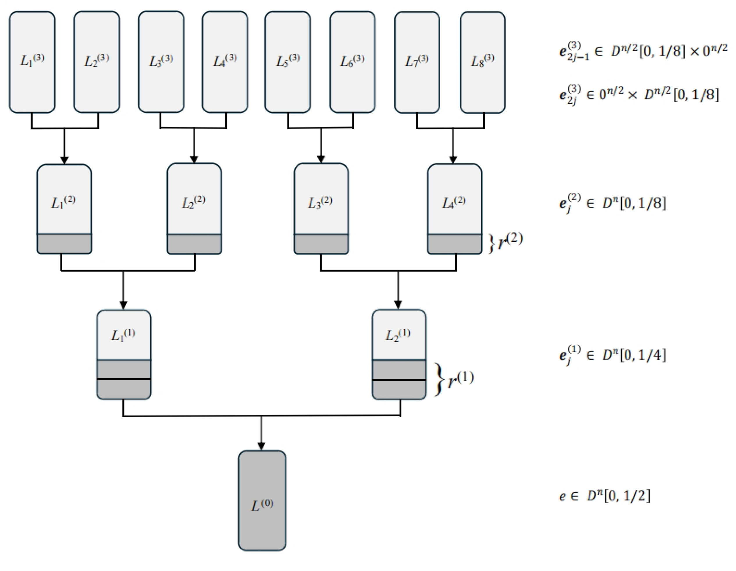
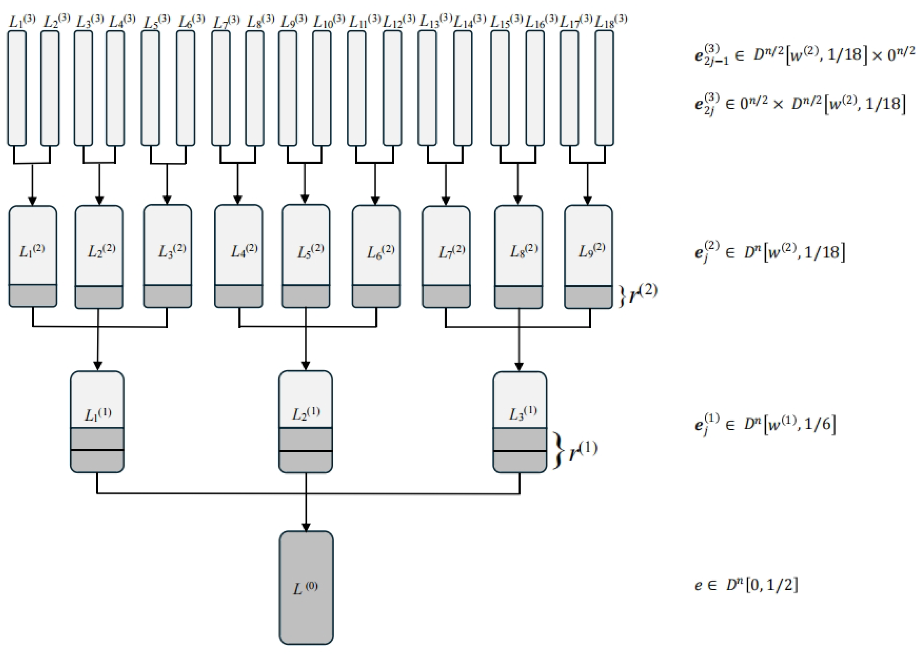
The proposed classical algorithm, which we refer to as TER, employs a ternary tree structure as illustrated in Figure 2. We encourage the reader to consult the figure for a clearer understanding of the algorithmic workflow. The tree has a depth of 3—a value determined through numerical optimization to be optimal for TER (see Appendix A for details).

For clarity, we consider a subset-sum instance $(\mathbf{a},s)\in {\left({\mathbb{Z}}_N\right)}^{n+1}$ with a solution $\mathbf{e}\in D^n[0,1/2]$. The key idea is to represent $\mathbf{e}$ as a sum of three vectors in $D^n$, i.e.,

$$\mathbf{e}={\mathbf{e}}_1^{\left(1\right)}+{\mathbf{e}}_2^{\left(1\right)}+{\mathbf{e}}_3^{\left(1\right)}$$

where ${\mathbf{e}}_1^{\left(1\right)},{\mathbf{e}}_2^{\left(1\right)},{\mathbf{e}}_3^{\left(1\right)}\in D^n[w^{\left(1\right)},1/6]$. This means each of these three vectors contains exactly $w^{\left(1\right)}n$ entries equal to $-1$, $(1/6+w^{\left(1\right)})n$ entries equal to 1, and $(5/6-2w^{\left(1\right)})n$ entries equal to 0.

We begin by computing the number of representations and establishing the parameter $w^{\left(1\right)}$. For each 1-coordinate $e_k$ in $\mathbf{e}$, its decomposition via the k-th coordinates of ${\mathbf{e}}_1^{\left(1\right)},{\mathbf{e}}_2^{\left(1\right)},{\mathbf{e}}_3^{\left(1\right)}$ must be one of

$$1+0+0,0+1+0,0+0+1,1+1+(-1),1+(-1)+1,(-1)+1+1.$$

Let ${ϵ}_1^{\left(1\right)}n$ denote the number of representations for each of the last three types. The total number of representations for the first three types is equal to $(1/2-3{ϵ}_1^{\left(1\right)})n$, because $\mathbf{e}$ has $n/2$ 1-coordinates.

For each 0-coordinate $e_k$ in $\mathbf{e}$, its decomposition via the k-th coordinates of ${\mathbf{e}}_1^{\left(1\right)},{\mathbf{e}}_2^{\left(1\right)},{\mathbf{e}}_3^{\left(1\right)}$ must be one of

$$0+1+(-1),0+(-1)+1,1+0+(-1),(-1)+0+1,1+(-1)+0,(-1)+1+0,$$

excluding the trivial case $0+0+0$. Let ${ϵ}_0^{\left(1\right)}n$ denote the number of each of these six nontrivial representations.

Table 3. Count of different level-1 representations.

	Representations	Count
1-coordinates	$1+0+0$	$(1/6-{ϵ}_1^{\left(1\right)})n$
	$0+1+0$	$(1/6-{ϵ}_1^{\left(1\right)})n$
	$0+0+1$	$(1/6-{ϵ}_1^{\left(1\right)})n$
	$1+1+(-1)$	${ϵ}_1^{\left(1\right)}n$
	$1+(-1)+1$	${ϵ}_1^{\left(1\right)}n$
	$(-1)+1+1$	${ϵ}_1^{\left(1\right)}n$
0-coordinates	$0+1+(-1)$	${ϵ}_0^{\left(1\right)}n$
	$0+(-1)+1$	${ϵ}_0^{\left(1\right)}n$
	$1+0+(-1)$	${ϵ}_0^{\left(1\right)}n$
	$(-1)+0+1$	${ϵ}_0^{\left(1\right)}n$
	$1+(-1)+0$	${ϵ}_0^{\left(1\right)}n$
	$(-1)+1+0$	${ϵ}_0^{\left(1\right)}n$
	$0+0+0$	$(1/2-6{ϵ}_0^{\left(1\right)})n$

summarizes the counts for each type of level-1 representation.

The total number of representations is given by

$$\begin{array}{cc}\hfill R^{\left(1\right)}& =\left({\displaystyle \genfrac{}{}{0pt}{}{n/2}{{ϵ}_1^{\left(1\right)}n,{ϵ}_1^{\left(1\right)}n,{ϵ}_1^{\left(1\right)}n,(1/6-{ϵ}_1^{\left(1\right)})n,(1/6-{ϵ}_1^{\left(1\right)})n,·}}\right)\hfill \\ \hfill & \times \left({\displaystyle \genfrac{}{}{0pt}{}{n/2}{{ϵ}_0^{\left(1\right)}n,{ϵ}_0^{\left(1\right)}n,{ϵ}_0^{\left(1\right)}n,{ϵ}_0^{\left(1\right)}n,{ϵ}_0^{\left(1\right)}n,{ϵ}_0^{\left(1\right)}n,·}}\right),\hfill \end{array}$$

where the two factors, respectively, account for the number of representations for 1-coordinates and 0-coordinates in the vector $\mathbf{e}$.

The number of $(-1)$-coordinates of ${\mathbf{e}}_j^{\left(1\right)}$ for $j=1,2,3$ is $({ϵ}_1^{\left(1\right)}+2{ϵ}_0^{\left(1\right)})n,$ and the number of 1-coordinates is $(1/6+{ϵ}_1^{\left(1\right)}+2{ϵ}_0^{\left(1\right)})n.$ Let $w^{\left(1\right)}={ϵ}_1^{\left(1\right)}+2{ϵ}_0^{\left(1\right)}$, then ${\mathbf{e}}_j^{\left(1\right)}\in D^n\left[w^{\left(1\right)},1/6\right]$ for $j=1,2,3$.

To capture a representation of $\mathbf{e}$, we choose a modulus $2^{r^{\left(1\right)}}$ where $r^{\left(1\right)}=\lfloor {\displaystyle \frac{1}{2}}{log}_2{R}^{\left(1\right)}\rfloor$, and random targets $s_1^{\left(1\right)},s_2^{\left(1\right)}\in \{0,1,\dots ,2^{r^{\left(1\right)}}-1\}$. We then define the lists:

$$\begin{array}{cc}\hfill L_1^{\left(1\right)}& =\left\{\left({\mathbf{e}}_1^{\left(1\right)},\langle \mathbf{a},{\mathbf{e}}_1^{\left(1\right)}\rangle \right)\in D^n[w^{\left(1\right)},1/6]\times {\mathbb{Z}}_N\mid \langle \mathbf{a},{\mathbf{e}}_1^{\left(1\right)}\rangle \equiv s_1^{\left(1\right)}mod{2}^{r^{\left(1\right)}}\right\},\hfill \\ \hfill L_2^{\left(1\right)}& =\left\{\left({\mathbf{e}}_2^{\left(1\right)},\langle \mathbf{a},{\mathbf{e}}_2^{\left(1\right)}\rangle \right)\in D^n[w^{\left(1\right)},1/6]\times {\mathbb{Z}}_N\mid \langle \mathbf{a},{\mathbf{e}}_2^{\left(1\right)}\rangle \equiv s_2^{\left(1\right)}mod{2}^{r^{\left(1\right)}}\right\},\hfill \\ \hfill L_3^{\left(1\right)}& =\left\{\left({\mathbf{e}}_3^{\left(1\right)},\langle \mathbf{a},{\mathbf{e}}_3^{\left(1\right)}\rangle \right)\in D^n[w^{\left(1\right)},1/6]\times {\mathbb{Z}}_N\mid \langle \mathbf{a},{\mathbf{e}}_3^{\left(1\right)}\rangle \equiv s_3^{\left(1\right)}mod{2}^{r^{\left(1\right)}}\right\},\hfill \end{array}$$

(1)

where $s_3^{\left(1\right)}=s-s_1^{\left(1\right)}-s_2^{\left(1\right)}$.

A valid solution is found when $\langle \mathbf{a},{\mathbf{e}}_1^{\left(1\right)}\rangle +\langle \mathbf{a},{\mathbf{e}}_2^{\left(1\right)}\rangle =\langle \mathbf{a},{\mathbf{e}}_3^{\left(1\right)}\rangle$ and ${\mathbf{e}}_1^{\left(1\right)}+{\mathbf{e}}_2^{\left(1\right)}+{\mathbf{e}}_3^{\left(1\right)}\in D^n[0,1/2]$. If no collision occurs, new values $(s_1^{\left(1\right)},s_2^{\left(1\right)})$ are sampled. The failure probability becomes negligible after polynomially many attempts.

The expected size of each list $L_j^{\left(1\right)}$$(j=1,2,3)$ is

$$\mathbb{E}\left[|L_j^{\left(1\right)}|\right]={\displaystyle \frac{\left(\genfrac{}{}{0pt}{}{n}{w^{\left(1\right)}n,(1/6+w^{\left(1\right)})n,·}\right)}{\sqrt{R^{\left(1\right)}}}}.$$

These lists are constructed recursively. For example, to build $L_1^{\left(1\right)}$, we represent ${\mathbf{e}}_1^{\left(1\right)}\in D^n[w^{\left(1\right)},1/6]$ as ${\mathbf{e}}_1^{\left(1\right)}={\mathbf{e}}_1^{\left(2\right)}+{\mathbf{e}}_2^{\left(2\right)}+{\mathbf{e}}_3^{\left(2\right)}$ with ${\mathbf{e}}_1^{\left(2\right)},{\mathbf{e}}_2^{\left(2\right)},{\mathbf{e}}_3^{\left(2\right)}\in D^n[w^{\left(2\right)},1/18]$.

Let ${ϵ}_1^{\left(2\right)}n$ count each of the representations $1+1+(-1)$, $1+(-1)+1$, and $(-1)+1+1$ for the 1-coordinates of ${\mathbf{e}}_1^{\left(1\right)}$, and ${ϵ}_0^{\left(2\right)}n$ count each of the six nontrivial representations of the 0-coordinates. For the $(-1)$-coordinates, the representations are

$$(-1)+0+0,0+(-1)+0,0+0+(-1),1+(-1)+(-1),(-1)+1+(-1),(-1)+(-1)+1.$$

Let ${ϵ}_{-1}^{\left(2\right)}n$ count each of the last three types.

Table 4. Count of different level-2 representations.

	Representations	Count
1-coordinates	$1+0+0$	$(1/18+w^{\left(1\right)}/3-{ϵ}_1^{\left(2\right)})n$
	$0+1+0$	$(1/18+w^{\left(1\right)}/3-{ϵ}_1^{\left(2\right)})n$
	$0+0+1$	$(1/18+w^{\left(1\right)}/3-{ϵ}_1^{\left(2\right)})n$
	$1+1+(-1)$	${ϵ}_1^{\left(2\right)}n$
	$1+(-1)+1$	${ϵ}_1^{\left(2\right)}n$
	$(-1)+1+1$	${ϵ}_1^{\left(2\right)}n$
0-coordinates	$0+1+(-1)$	${ϵ}_0^{\left(2\right)}n$
	$0+(-1)+1$	${ϵ}_0^{\left(2\right)}n$
	$1+0+(-1)$	${ϵ}_0^{\left(2\right)}n$
	$(-1)+0+1$	${ϵ}_0^{\left(2\right)}n$
	$1+(-1)+0$	${ϵ}_0^{\left(2\right)}n$
	$(-1)+1+0$	${ϵ}_0^{\left(2\right)}n$
	$0+0+0$	$(5/6-2w^{\left(1\right)}-6{ϵ}_0^{\left(2\right)})n$
$-1$-coordinates	$(-1)+0+0$	$(w^{\left(1\right)}/3-{ϵ}_{-1}^{\left(2\right)})n$
	$0+(-1)+0$	$(w^{\left(1\right)}/3-{ϵ}_{-1}^{\left(2\right)})n$
	$0+0+(-1)$	$(w^{\left(1\right)}/3-{ϵ}_{-1}^{\left(2\right)})n$
	$1+(-1)+(-1)$	${ϵ}_{-1}^{\left(2\right)}n$
	$(-1)+1+(-1)$	${ϵ}_{-1}^{\left(2\right)}n$
	$(-1)+(-1)+1$	${ϵ}_{-1}^{\left(2\right)}n$

provides the counts for each type of level-2 representation.

The number of representations at this level is

$$\begin{array}{cc}\hfill R^{\left(2\right)}& =\left({\displaystyle \genfrac{}{}{0pt}{}{(1/6+w^{\left(1\right)})n}{{ϵ}_1^{\left(2\right)}n,{ϵ}_1^{\left(2\right)}n,{ϵ}_1^{\left(2\right)}n,(1/18+w^{\left(1\right)}/3-{ϵ}_1^{\left(2\right)})n,(1/18+w^{\left(1\right)}/3-{ϵ}_1^{\left(2\right)})n,·}}\right)\hfill \\ \hfill & \times \left({\displaystyle \genfrac{}{}{0pt}{}{(5/6-2w^{\left(1\right)})n}{{ϵ}_0^{\left(2\right)}n,{ϵ}_0^{\left(2\right)}n,{ϵ}_0^{\left(2\right)}n,{ϵ}_0^{\left(2\right)}n,{ϵ}_0^{\left(2\right)}n,{ϵ}_0^{\left(2\right)}n,·}}\right)\hfill \\ \hfill & \times \left({\displaystyle \genfrac{}{}{0pt}{}{w^{\left(1\right)}n}{{ϵ}_{-1}^{\left(2\right)}n,{ϵ}_{-1}^{\left(2\right)}n,{ϵ}_{-1}^{\left(2\right)}n,(w^{\left(1\right)}/3-{ϵ}_{-1}^{\left(2\right)})n,(w^{\left(1\right)}/3-{ϵ}_{-1}^{\left(2\right)})n,·}}\right).\hfill \end{array}$$

The number of $(-1)$-coordinates of ${\mathbf{e}}_j^{\left(2\right)}$ for $j=1,2,3$ is calculated as

$$\begin{array}{cc}\hfill & \left(w^{\left(1\right)}/3-{ϵ}_{-1}^{\left(2\right)}+2{ϵ}_{-1}^{\left(2\right)}+2{ϵ}_0^{\left(2\right)}+{ϵ}_1^{\left(2\right)}\right)n\hfill \\ \hfill =& \left({ϵ}_1^{\left(1\right)}/3+2{ϵ}_0^{\left(1\right)}/3+{ϵ}_{-1}^{\left(2\right)}+{ϵ}_1^{\left(2\right)}+2{ϵ}_0^{\left(2\right)}\right)n,\hfill \end{array}$$

and the number of 1-coordinates of ${\mathbf{e}}_j^{\left(1\right)}$ for $j=1,2,3$ is calculated as

$$\begin{array}{cc}\hfill & \left(1/18+w^{\left(1\right)}/3-{ϵ}_1^{\left(2\right)}+2{ϵ}_1^{\left(2\right)}+2{ϵ}_0^{\left(2\right)}+{ϵ}_{-1}^{\left(2\right)}\right)n\hfill \\ \hfill =& \left(1/18+{ϵ}_1^{\left(1\right)}/3+2{ϵ}_0^{\left(1\right)}/3+{ϵ}_{-1}^{\left(2\right)}+{ϵ}_1^{\left(2\right)}+2{ϵ}_0^{\left(2\right)}\right)n.\hfill \end{array}$$

Let $w^{\left(2\right)}={ϵ}_1^{\left(1\right)}/3+2{ϵ}_0^{\left(1\right)}/3+{ϵ}_{-1}^{\left(2\right)}+{ϵ}_1^{\left(2\right)}+2{ϵ}_0^{\left(2\right)}$, then ${\mathbf{e}}_j^{\left(2\right)}\in D^n[w^{\left(2\right)},1/18]$ for $j=1,2,3$.

Let $r^{\left(2\right)}=\lfloor {\displaystyle \frac{1}{2}}{log}_2{R}^{\left(2\right)}\rfloor$ and choose random targets $s_j^{\left(2\right)}\in \{0,1,\dots ,2^{r^{\left(2\right)}}-1\}$ for $j\in \{1,2,4,5,7,8\}$. We define

$$L_j^{\left(2\right)}=\left\{\left({\mathbf{e}}_j^{\left(2\right)},\langle \mathbf{a},{\mathbf{e}}_j^{\left(2\right)}\rangle \right)\in D^n\left[w^{\left(2\right)},1/18\right]\times {\mathbb{Z}}_N\mid \langle \mathbf{a},{\mathbf{e}}_j^{\left(2\right)}\rangle \equiv s_j^{\left(2\right)}mod{2}^{r^{\left(2\right)}}\right\},$$

for $j\in \{1,\dots ,9\}$, where $s_{3k}^{\left(2\right)}=s_k^{\left(1\right)}-s_{3k-2}^{\left(2\right)}-s_{3k-1}^{\left(2\right)}$ for $k=1,2,3$.

The expected size of each $L_j^{\left(2\right)}$$(j\in \{1,\dots ,9\left\}\right)$ is

$$\mathbb{E}\left[|L_j^{\left(2\right)}|\right]={\displaystyle \frac{\left(\genfrac{}{}{0pt}{}{n}{w^{\left(2\right)}n,(1/18+w^{\left(2\right)})n,·}\right)}{\sqrt{R^{\left(2\right)}}}}.$$

The level-2 lists are built from the level-3 lists via a Meet-in-the-Middle approach.

$$\begin{array}{cc}\hfill L_{2j-1}^{\left(3\right)}& =\left\{\left({\mathbf{e}}_{2j-1}^{\left(3\right)},\langle \mathbf{a},{\mathbf{e}}_{2j-1}^{\left(3\right)}\rangle \right)\in D^{n/2}\left[w^{\left(2\right)},1/18\right]\times 0^{n/2}\times {\mathbb{Z}}_N\right\},\hfill \\ \hfill L_{2j}^{\left(3\right)}& =\left\{\left({\mathbf{e}}_{2j}^{\left(3\right)},\langle \mathbf{a},{\mathbf{e}}_{2j}^{\left(3\right)}\rangle \right)\in 0^{n/2}\times D^{n/2}\left[w^{\left(2\right)},1/18\right]\times {\mathbb{Z}}_N\right\},\hfill \end{array}$$

for $j\in \{1,\dots ,9\}$, each of size

$$\left({\displaystyle \genfrac{}{}{0pt}{}{n/2}{(w^{\left(2\right)}/2)n,(1/36+w^{\left(2\right)}/2)n,·}}\right).$$

Note that we employ the binary tree only for the top level, because the representation technique is not used in this level.

Algorithm 2 outlines the TER algorithm with a depth of 3. In summary, it recursively constructs three lists $L_1^{\left(1\right)},L_2^{\left(1\right)},L_3^{\left(1\right)}$ that are expected to contain a single representation of $\mathbf{e}$. Similar to the HGJ algorithm, this algorithm executes the merge-and-filter operation repeatedly over several levels.

Consider three input distributions, $D_1=D^n\left[{\alpha }_1,{\beta }_1\right]$, $D_2=D^n\left[{\alpha }_2,{\beta }_2\right]$ and $D_3=D^n\left[{\alpha }_3,{\beta }_3\right]$, with a target distribution $D=D^n\left[\alpha ,\beta \right]$. Given three lists $L_1\in D_1^{|L_1|}$, $L_2\in D_2^{|L_2|}$ and $L_3\in D_2^{|L_3|}$, we define the following:

• The merged list

  $$\begin{array}{c}{L}_m=\{({\mathbf{e}}_1+{\mathbf{e}}_2+{\mathbf{e}}_3,\langle \mathbf{a},{\mathbf{e}}_1+{\mathbf{e}}_2+{\mathbf{e}}_3\rangle )\mid \hfill \\ \hfill \hspace{1em}\hspace{1em}\hspace{1em}\hspace{1em}\hspace{1em}\hspace{1em}\hspace{1em}\hspace{1em}\hspace{1em}{\mathbf{e}}_1\in L_1,{\mathbf{e}}_2\in L_2,{\mathbf{e}}_3\in L_3,\langle \mathbf{a},{\mathbf{e}}_1+{\mathbf{e}}_2+{\mathbf{e}}_3\rangle \equiv tmodM\},\end{array}$$

  (2)

  where $0\le t<M$ is an arbitrary integer,
• The filtered list $L_f=(L_m\cap D)\subseteq L_m,$ containing the vectors with the target distribution.

Algorithm 2 TER with a depth of 3

Input:  The random subset-sum instance $(\mathbf{a},s)\in {\left({\mathbb{Z}}_N\right)}^{n+1}$ Parameters:  ${ϵ}_1^{\left(1\right)},{ϵ}_0^{\left(1\right)},{ϵ}_1^{\left(2\right)},{ϵ}_0^{\left(2\right)},{ϵ}_{-1}^{\left(2\right)}$ that need to be optimized. Output:  A solution $\mathbf{e}\in D^n\left[0,1/2\right]$ or ⊥ if no solution is found.   1: Construct all level-3 lists $L_j^{\left(3\right)}$ for $j\in \{1,\dots ,18\}.$   2: Compute $L_j^{\left(2\right)}$ from $L_{2j-1}^{\left(3\right)},L_{2j}^{\left(3\right)}$ for $j\in \{1,\dots ,9\}.$   3: for $i=1$ down to 0 do   4:       for $j=1$ to $3^i$ do   5:             Construct $L_j^{\left(i\right)}$ from $L_{3j-2}^{(i+1)},L_{3j-1}^{(i+1)},L_{3j}^{(i+1)}$.   6:       end for   7: end for   8: if  $L_1^{\left(0\right)}\ne \varnothing$then   9:       return any $\mathbf{e}\in L_1^{\left(0\right)}$ 10: else 11:       return ⊥ 12: end if

Similar to the standard subset-sum assumption, our heuristic assumes that elements in $L_f$ are independently and uniformly sampled from the distribution D.

Heuristic 2.

Suppose the input vectors are uniformly distributed over $D_1\times D_2\times D_3$. Then the filtered pairs of vectors are also uniformly distributed over the target set D—or more precisely, over the subset of vectors in D that satisfy the given modular constraint.

By Heuristic 2, the expected sizes of the merged list is given by $|L_m|=(|L_1|·|L_2|·|L_3\left|\right)/M$, and the average size of the filtered list $L_f$ equals $|L_m|·\mathrm{pf}$, where pf denotes the probability that a uniformly random triple $({\mathbf{e}}_1,{\mathbf{e}}_2,{\mathbf{e}}_3)$ from $D_1\times D_2\times D_3$ satisfies $({\mathbf{e}}_1+{\mathbf{e}}_2+{\mathbf{e}}_3)\in D.$

Theorem 1.

Let $(\mathbf{a},s)\in {\left({\mathbb{Z}}_N\right)}^{n+1}$ be a random subset-sum instance whose solution is a vector $\mathbf{e}\in D^n\left[0,1/2\right]$. Under Heuristic 2, Algorithm 2 finds $\mathbf{e}$ in time $\widetilde{𝒪}\left(2^{0.2400n}\right)$ and space $\widetilde{𝒪}\left(2^{0.2221n}\right)$.

Proof. 

For each level $i\in \{1,2,3\}$, the size of the corresponding lists is denoted by $L^{\left(i\right)}$. Under Heuristic 2, the list sizes concentrate sharply around their expectations, leading to the expressions

$$\begin{array}{cc}\hfill L^{\left(1\right)}& =\left({\displaystyle \genfrac{}{}{0pt}{}{n}{w^{\left(1\right)}n,(1/6+w^{\left(1\right)})n,·}}\right)/\sqrt{R^{\left(1\right)}},\hfill \\ \hfill L^{\left(2\right)}& =\left({\displaystyle \genfrac{}{}{0pt}{}{n}{w^{\left(2\right)}n,(1/18+w^{\left(2\right)})n,·}}\right)/\sqrt{R^{\left(2\right)}},\hfill \\ \hfill L^{\left(3\right)}& =\left({\displaystyle \genfrac{}{}{0pt}{}{n/2}{(w^{\left(2\right)}/2)n,(1/36+w^{\left(2\right)}/2)n,·}}\right).\hfill \end{array}$$

where

$$\begin{array}{cc}\hfill w^{\left(1\right)}& ={ϵ}_1^{\left(1\right)}+2{ϵ}_0^{\left(1\right)},\hfill \\ \hfill w^{\left(2\right)}& ={ϵ}_1^{\left(1\right)}/3+2{ϵ}_0^{\left(1\right)}/3+{ϵ}_{-1}^{\left(2\right)}+{ϵ}_1^{\left(2\right)}+2{ϵ}_0^{\left(2\right)},\hfill \\ \hfill R^{\left(1\right)}& =\left({\displaystyle \genfrac{}{}{0pt}{}{n/2}{{ϵ}_1^{\left(1\right)}n,{ϵ}_1^{\left(1\right)}n,{ϵ}_1^{\left(1\right)}n,(1/6-{ϵ}_1^{\left(1\right)})n,(1/6-{ϵ}_1^{\left(1\right)})n,·}}\right)\hfill \\ \hfill & \times \left({\displaystyle \genfrac{}{}{0pt}{}{n/2}{{ϵ}_0^{\left(1\right)}n,{ϵ}_0^{\left(1\right)}n,{ϵ}_0^{\left(1\right)}n,{ϵ}_0^{\left(1\right)}n,{ϵ}_0^{\left(1\right)}n,{ϵ}_0^{\left(1\right)}n,·}}\right),\hfill \\ \hfill R^{\left(2\right)}& =\left({\displaystyle \genfrac{}{}{0pt}{}{(1/6+w^{\left(1\right)})n}{{ϵ}_1^{\left(2\right)}n,{ϵ}_1^{\left(2\right)}n,{ϵ}_1^{\left(2\right)}n,(1/18+w^{\left(1\right)}/3-{ϵ}_1^{\left(2\right)})n,(1/18+w^{\left(1\right)}/3-{ϵ}_1^{\left(2\right)})n,·}}\right)\hfill \\ \hfill & \times \left({\displaystyle \genfrac{}{}{0pt}{}{(5/6-2w^{\left(1\right)})n}{{ϵ}_0^{\left(2\right)}n,{ϵ}_0^{\left(2\right)}n,{ϵ}_0^{\left(2\right)}n,{ϵ}_0^{\left(2\right)}n,{ϵ}_0^{\left(2\right)}n,{ϵ}_0^{\left(2\right)}n,·}}\right)\hfill \\ \hfill & \times \left({\displaystyle \genfrac{}{}{0pt}{}{w^{\left(1\right)}n}{{ϵ}_{-1}^{\left(2\right)}n,{ϵ}_{-1}^{\left(2\right)}n,{ϵ}_{-1}^{\left(2\right)}n,(w^{\left(1\right)}/3-{ϵ}_{-1}^{\left(2\right)})n,(w^{\left(1\right)}/3-{ϵ}_{-1}^{\left(2\right)})n,·}}\right),\hfill \end{array}$$

and ${ϵ}_1^{\left(1\right)},{ϵ}_0^{\left(1\right)},{ϵ}_1^{\left(2\right)},{ϵ}_0^{\left(2\right)},{ϵ}_{-1}^{\left(2\right)}$ are parameters to be optimized.

Based on the preceding analysis, the time complexity of Algorithm 2 can be derived as follows:

$$max\left(L^{\left(3\right)},{\displaystyle \frac{{\left(L^{\left(3\right)}\right)}^2}{\sqrt{R^{\left(2\right)}}}},{\displaystyle \frac{{\left(L^{\left(2\right)}\right)}^3}{\sqrt{R^{\left(1\right)}/R^{\left(2\right)}}}},{\displaystyle \frac{{\left(L^{\left(1\right)}\right)}^3}{N/\sqrt{R^{\left(1\right)}}}}\right),$$

and the space complexity is $max\left(L^{\left(3\right)},L^{\left(2\right)},L^{\left(1\right)}\right)$. Let us focus on the asymptotic exponent in ${log}_2$ and relative to n. Denote $l^{\left(i\right)}={log}_2\left(L^{\left(i\right)}\right)/n$ for $i=1,2,3$. Recall that $r^{\left(1\right)}=\lfloor {\displaystyle \frac{1}{2}}{log}_2{R}^{\left(1\right)}\rfloor$ and $r^{\left(2\right)}=\lfloor {\displaystyle \frac{1}{2}}{log}_2{R}^{\left(2\right)}\rfloor$. Computing the time complexity essentially amounts to solving the following optimization problem, where the objective function is

$$max\left(l^{\left(3\right)},2l^{\left(3\right)}-r^{\left(2\right)}/n,3l^{\left(2\right)}-(r^{\left(1\right)}-r^{\left(2\right)})/n,3l^{\left(1\right)}-(1-r^{\left(1\right)}/n)\right),$$

subject to the following constraints:

$$\begin{array}{cc}\hfill l^{\left(1\right)}& =H(1/6+w^{\left(1\right)},w^{\left(1\right)})-r^{\left(1\right)}/n,\hfill \\ \hfill l^{\left(2\right)}& =H(1/18+w^{\left(2\right)},w^{\left(2\right)})-r^{\left(2\right)}/n,\hfill \\ \hfill l^{\left(3\right)}& =H(1/18+w^{\left(2\right)},w^{\left(2\right)})/2,\hfill \\ \hfill w^{\left(1\right)}& ={ϵ}_1^{\left(1\right)}+2{ϵ}_0^{\left(1\right)},\hfill \\ \hfill w^{\left(2\right)}& ={ϵ}_1^{\left(1\right)}/3+2{ϵ}_0^{\left(1\right)}/3+{ϵ}_{-1}^{\left(2\right)}+{ϵ}_1^{\left(2\right)}+2{ϵ}_0^{\left(2\right)},\hfill \\ \hfill {\displaystyle \frac{2r^{\left(1\right)}}{n}}& =H(2{ϵ}_1^{\left(1\right)},2{ϵ}_1^{\left(1\right)},2{ϵ}_1^{\left(1\right)},1/3-2{ϵ}_1^{\left(1\right)},1/3-2{ϵ}_1^{\left(1\right)},·)/2\hfill \\ \hfill & +H(2{ϵ}_0^{\left(1\right)},2{ϵ}_0^{\left(1\right)},2{ϵ}_0^{\left(1\right)},2{ϵ}_0^{\left(1\right)},2{ϵ}_0^{\left(1\right)},2{ϵ}_0^{\left(1\right)},·)/2,\hfill \\ \hfill {\displaystyle \frac{2r^{\left(2\right)}}{n}}& =H\left({\displaystyle \frac{{ϵ}_1^{\left(2\right)}}{1/6+w^{\left(1\right)}}},{\displaystyle \frac{{ϵ}_1^{\left(2\right)}}{1/6+w^{\left(1\right)}}},{\displaystyle \frac{{ϵ}_1^{\left(2\right)}}{1/6+w^{\left(1\right)}}},1/3-{\displaystyle \frac{{ϵ}_1^{\left(2\right)}}{1/6+w^{\left(1\right)}}},1/3-{\displaystyle \frac{{ϵ}_1^{\left(2\right)}}{1/6+w^{\left(1\right)}}},·\right)\hfill \\ \hfill & \times (1/6+w^{\left(1\right)})\hfill \\ \hfill & +H\left({\displaystyle \frac{{ϵ}_0^{\left(2\right)}}{5/6-2w^{\left(1\right)}}},{\displaystyle \frac{{ϵ}_0^{\left(2\right)}}{5/6-2w^{\left(1\right)}}},{\displaystyle \frac{{ϵ}_0^{\left(2\right)}}{5/6-2w^{\left(1\right)}}},{\displaystyle \frac{{ϵ}_0^{\left(2\right)}}{5/6-2w^{\left(1\right)}}},{\displaystyle \frac{{ϵ}_0^{\left(2\right)}}{5/6-2w^{\left(1\right)}}},{\displaystyle \frac{{ϵ}_0^{\left(2\right)}}{5/6-2w^{\left(1\right)}}},·\right)\hfill \\ \hfill & \times (5/6-2w^{\left(1\right)})\hfill \\ \hfill & +H\left({\displaystyle \frac{{ϵ}_{-1}^{\left(2\right)}}{w^{\left(1\right)}}},{\displaystyle \frac{{ϵ}_{-1}^{\left(2\right)}}{w^{\left(1\right)}}},{\displaystyle \frac{{ϵ}_{-1}^{\left(2\right)}}{w^{\left(1\right)}}},1/3-{\displaystyle \frac{{ϵ}_{-1}^{\left(2\right)}}{w^{\left(1\right)}}},1/3-{\displaystyle \frac{{ϵ}_{-1}^{\left(2\right)}}{w^{\left(1\right)}}},·\right)\times w^{\left(1\right)}.\hfill \end{array}$$

Note that Lemma 1 is applied when computing the exponents of the constraints.

Numerical optimization yields the parameters

$${ϵ}_0^{\left(1\right)}=0.0066,{ϵ}_1^{\left(1\right)}=0.0024,{ϵ}_0^{\left(2\right)}=0.0004,{ϵ}_1^{\left(2\right)}=0.0001,{ϵ}_{-1}^{\left(2\right)}=0.0000,$$

$$w^{\left(1\right)}=0.0156,w^{\left(2\right)}=0.0059.$$

This results in

$$R^{\left(1\right)}=2^{1.1473n},R^{\left(2\right)}=2^{0.3396n},$$

which in turn yield list sizes

$$L^{\left(3\right)}=2^{0.1922n},L^{\left(2\right)}=2^{0.2147n},L^{\left(1\right)}=2^{0.2221n},L^{\left(0\right)}=1.$$

The time complexity is $\widetilde{𝒪}\left(2^{0.2400n}\right)$, determined by the merged list size, and the space complexity is $\widetilde{𝒪}\left(2^{0.2221n}\right)$, governed by the filtered list size.    □

3.2. Rigorous Analysis of TER

In this subsection, we establish rigorous foundations for Heuristic 2 and present a provable variant of TER that eliminates heuristic assumptions. Our analysis relies on distributional properties of modular sums, as captured by the following fundamental result (Theorem 3.2 in [46]).

Theorem 2.

For any set $\mathcal{B}\subset {\mathbb{Z}}_M^n$, the identity

$${\displaystyle \frac{1}{M^n}}\sum _{\mathbf{a}\in {\mathbb{Z}}_M^n}\sum _{c\in {\mathbb{Z}}_M}{\left(P_{\mathbf{a}}(\mathcal{B},c)-{\displaystyle \frac{1}{M}}\right)}^2={\displaystyle \frac{M-1}{M\left|\mathcal{B}\right|}}$$

(3)

holds, where $P_{\mathbf{a}}(\mathcal{B},c)$ denotes the probability that $\mathbf{a}·\mathbf{x}:=\langle \mathbf{a},\mathbf{x}\rangle \equiv c(modM)$ for a random $\mathbf{x}$ drawn uniformly from $\mathcal{B}$, i.e.,

$$P_{\mathbf{a}}(\mathcal{B},c)={\displaystyle \frac{1}{\left|\mathcal{B}\right|}}\left|\left\{(x_1,\dots ,x_n)\in \mathcal{B}\mathrm{s}.\mathrm{t}.\mathbf{a}·\mathbf{x}\equiv cmodM\right\}\right|.$$

The left-hand side of Equation (3) represents the average squared deviation from uniformity across all coefficient vectors $\mathbf{a}=(a_1,\dots ,a_n)$ and residues $c\in {\mathbb{Z}}_M$. This quantity measures the overall non-uniformity of the distribution. The right-hand side being constant for fixed $\left|\mathcal{B}\right|$ implies that if certain subset-sum instances exhibit significant deviation from uniformity, others must be exceptionally uniform to maintain the average.

We now extend this result to the Cartesian product setting relevant to our decomposition approach.

Theorem 3.

For any sets ${\mathcal{B}}_1,{\mathcal{B}}_2\subset {\mathbb{Z}}_M^n$ and the same coefficient vector $\mathbf{a}\in {\mathbb{Z}}_M^n$, the identity

$${\displaystyle \frac{1}{M^n}}\sum _{\mathbf{a}\in {\mathbb{Z}}_M^n}\sum _{(c_1,c_2)\in {\mathbb{Z}}_M^2}{\left(P_{\mathbf{a}}({\mathcal{B}}_1\times {\mathcal{B}}_2,c_1,c_2)-{\displaystyle \frac{1}{M^2}}\right)}^2={\displaystyle \frac{{(M-1)}^2}{M^2|{\mathcal{B}}_1\left|\right|{\mathcal{B}}_2|}}$$

(4)

holds, where $P_{\mathbf{a}}({\mathcal{B}}_1\times {\mathcal{B}}_2,c_1,c_2)$ denotes the probability that $\mathbf{a}·\mathbf{x}\equiv c_1(modM)$ and $\mathbf{a}·\mathbf{y}\equiv c_2(modM)$ for random $(\mathbf{x},\mathbf{y})$ drawn uniformly from ${\mathcal{B}}_1\times {\mathcal{B}}_2$.

Proof. 

See Appendix C for the full proof.    □

We now analyze pathological instances that cause TER to fail. During ternary decomposition (e.g., representing $\mathbf{e}$ as ${\mathbf{e}}_1^{\left(1\right)}+{\mathbf{e}}_2^{\left(1\right)}+{\mathbf{e}}_3^{\left(1\right)}$), certain coefficient vectors—such as $\mathbf{a}=(0,\dots ,0)$—prevent constructing valid level-1 lists (Equation (1)) with random targets $s_1^{\left(1\right)},s_2^{\left(1\right)}$ due to sparse residue coverage.

Let ${\mathcal{B}}_1$ and ${\mathcal{B}}_2$ denote the vector sets in the first two parts of the ternary decomposition. We quantify how many residue pairs $(s_1^{\left(1\right)},s_2^{\left(1\right)})\in {\mathbb{Z}}_M^2$ remain uncovered by ${\mathcal{B}}_1\times {\mathcal{B}}_2$. For parameter $\mathrm{\Lambda }>0$, define an instance as Type I bad if either ${\mathcal{B}}_1$ covers fewer than $M/\mathrm{\Lambda }$ residues or ${\mathcal{B}}_2$ covers fewer than $M/\mathrm{\Lambda }$ residues.

For such bad instances, at least $(\mathrm{\Lambda }-1)M/\mathrm{\Lambda }$ residues lead to zero probability: $P_{\mathbf{a}}({\mathcal{B}}_1,s_1^{\left(1\right)})=0$ or $P_{\mathbf{a}}({\mathcal{B}}_2,s_2^{\left(1\right)})=0$. We now establish a lower bound for the variance under bad instances. Without loss of generality, assume that ${\mathcal{B}}_1$ covers fewer than $M/\mathrm{\Lambda }$ residues. For at least $(\mathrm{\Lambda }-1)M/\mathrm{\Lambda }$ uncovered residues $s_1^{\left(1\right)}$,

$${\left(P_{\mathbf{a}}({\mathcal{B}}_1,s_1^{\left(1\right)})P_{\mathbf{a}}({\mathcal{B}}_2,s_2^{\left(1\right)})-{\displaystyle \frac{1}{M^2}}\right)}^2={\displaystyle \frac{1}{M^4}}.$$

For the remaining at most $M/\mathrm{\Lambda }$ covered residues $s_1^{\left(1\right)}$, we consider the minimal uniformity scenario: each such residue has a probability of at least $\mathrm{\Lambda }/M$ (since the total probability sums to 1), and $P_{\mathbf{a}}({\mathcal{B}}_2,s_2^{\left(1\right)})$ is uniform. Then,

$${\left(P_{\mathbf{a}}({\mathcal{B}}_1,s_1^{\left(1\right)})P_{\mathbf{a}}({\mathcal{B}}_2,s_2^{\left(1\right)})-{\displaystyle \frac{1}{M^2}}\right)}^2\ge {\displaystyle \frac{{(\mathrm{\Lambda }-1)}^2}{M^4}}.$$

Consequently, the lower bound for the variance is

$$\sum _{s_1^{\left(1\right)},s_2^{\left(1\right)}\in {\mathbb{Z}}_M}{\left(P_{\mathbf{a}}({\mathcal{B}}_1,s_1^{\left(1\right)})P_{\mathbf{a}}({\mathcal{B}}_2,s_2^{\left(1\right)})-{\displaystyle \frac{1}{M^2}}\right)}^2\ge {\displaystyle \frac{(\mathrm{\Lambda }-1)M^2}{\mathrm{\Lambda }}}·{\displaystyle \frac{1}{M^4}}+{\displaystyle \frac{M^2}{\mathrm{\Lambda }}}·{\displaystyle \frac{{(\mathrm{\Lambda }-1)}^2}{M^4}}={\displaystyle \frac{\mathrm{\Lambda }-1}{M^2}}.$$

Let $N_{\mathrm{I}}$ denote the number of Type I bad instances. By Theorem 3,

$$N_{\mathrm{I}}·{\displaystyle \frac{\mathrm{\Lambda }-1}{M^2}}\le M^n·{\displaystyle \frac{{(M-1)}^2}{M^2|{\mathcal{B}}_1\left|\right|{\mathcal{B}}_2|}}.$$

Since $|{\mathcal{B}}_1\left|\right|{\mathcal{B}}_2|\approx M^2$, the fraction of Type I bad instances is

$${\displaystyle \frac{N_I}{M^n}}\le {\displaystyle \frac{1}{\mathrm{\Lambda }-1}}.$$

Another failure mode occurs when intermediate lists grow beyond expected sizes, violating the complexity analysis in Theorem 1. We now rigorously analyze list sizes during TER’s execution.

Let $L_f$ be the filtered list in a merge-and-filter operation with distributions D. Let ${\mathcal{B}}_3$ denote all vectors with distribution D. We want $|L_f|\le \mathrm{\Lambda }|{\mathcal{B}}_3|/M$ for parameter $\mathrm{\Lambda }$. Define Type II bad instances as those where more than $M/\left(2\mathrm{\Lambda }\right)$ residues c satisfy $P\mathbf{a}({\mathcal{B}}_3,c)\ge \mathrm{\Lambda }/M$.

By Theorem 2,

$${\displaystyle \frac{N_{\mathrm{II}}}{M^n}}·{\displaystyle \frac{M}{2\mathrm{\Lambda }}}·{\displaystyle \frac{{(\mathrm{\Lambda }-1)}^2}{M^2}}\le {\displaystyle \frac{M-1}{M{\mathcal{B}}_3}}\le {\displaystyle \frac{1}{{\mathcal{B}}_3}},$$

where $N_{\mathrm{II}}$ counts Type II bad instances. Thus,

$$N_{\mathrm{II}}\le {\displaystyle \frac{2\mathrm{\Lambda }}{{(\mathrm{\Lambda }-1)}^2}}·{\displaystyle \frac{M}{{\mathcal{B}}_3}}·M^n\le {\displaystyle \frac{2\mathrm{\Lambda }}{{(\mathrm{\Lambda }-1)}^2}}·M^n.$$

The fraction of Type II bad instances is at most $\mathrm{\Lambda }/{(\mathrm{\Lambda }-1)}^2$.

Now consider the merged list size. Let $L_m$ be the merged list in a merge-and-filter operation (definition in Equation (2)). Let ${\mathcal{B}}_4$ contain all sums ${\mathbf{e}}_1+{\mathbf{e}}_2+{\mathbf{e}}_3$ without modular constraints. Decompose $M=M_1·M_2$, where $M_1$ represents active moduli from input lists and $M_2$ is the supplementary constraint introduced during $L_m$ construction.

Let $\sigma (modM)$ denote the target sum for elements in $L_m$, with ${\sigma }_L(mod{M}_1)$, ${\sigma }_M(mod{M}_1)$, ${\sigma }_R(mod{M}_1)$ representing partial sums from the three input lists, respectively, satisfying ${\sigma }_L+{\sigma }_M+{\sigma }_R\equiv \sigma (mod{M}_1)$.

The size of $L_m$ admits the bound

$$\begin{array}{cc}\hfill |L_m|& =\sum _{\begin{array}{c}{c}_1,c_2,c_3\in {\mathbb{Z}}_M\\ c_1+c_2+c_3\equiv \sigma (mod{M}_1)\end{array}}\left(\right|{\mathcal{B}}_4|·P_{\mathbf{a}}({\mathcal{B}}_4,c_1))·(|{\mathcal{B}}_4|·P_{\mathbf{a}}(\mathcal{B},c_2))·(|{\mathcal{B}}_4|·P_{\mathbf{a}}({\mathcal{B}}_4,c_3))\hfill \\ \hfill & \le {\left[\prod _{i=1}^3\sum _{\begin{array}{c}{c}_i\in {\mathbb{Z}}_M\\ c_i\equiv {\sigma }_i(mod{M}_1)\end{array}}\left(\right|{\mathcal{B}}_4{|·P_{\mathbf{a}}({\mathcal{B}}_4,c_i))}^3\right]}^{1/3}.\hfill \end{array}$$

To estimate this quantity, we require bounds on sums of the form

$$\sum _{\begin{array}{c}c\in {\mathbb{Z}}_M\\ c\equiv c_0(mod{M}_1)\end{array}}{P}_{\mathbf{a}}{(\mathcal{B},c)}^3.$$

We can extend the relation from Theorem 2 to third moments:

$${\displaystyle \frac{1}{M^n}}\sum _{\mathbf{a}\in {\mathbb{Z}}_M^n}\sum _{c\in {\mathbb{Z}}_M}{P}_{\mathbf{a}}{(\mathcal{B},c)}^3={\displaystyle \frac{M^2+3M\left|\mathcal{B}\right|-3M+{\left|\mathcal{B}\right|}^2-3\left|\mathcal{B}\right|+2}{M^2{\left|\mathcal{B}\right|}^2}}.$$

Define Type III bad instances as those where more than $M_1/\left(12\mathrm{\Lambda }\right)$ values $c_0$ satisfy

$$\sum _{\begin{array}{c}c\in {\mathbb{Z}}_M\\ c\equiv c_0(mod{M}_1)\end{array}}{P}_{\mathbf{a}}{({\mathcal{B}}_4,c)}^3\ge {\displaystyle \frac{{\mathrm{\Lambda }}^2}{M_1^3{M}_2}}.$$

Letting $N_{\mathrm{III}}$ count such instances,

$${\displaystyle \frac{N_{\mathrm{III}}}{M^n}}·{\displaystyle \frac{M_1}{12\mathrm{\Lambda }}}·{\displaystyle \frac{{\mathrm{\Lambda }}^2}{M_1^3{M}_2}}\le {\displaystyle \frac{M^2+3M|{\mathcal{B}}_4|-3M+|{\mathcal{B}}_4{|}^2-3\left|{\mathcal{B}}_4\right|+2}{M^2{\left|{\mathcal{B}}_4\right|}^2}}.$$

which implies

$$N_{\mathrm{III}}\le {\displaystyle \frac{12}{\mathrm{\Lambda }}}·{\displaystyle \frac{M^2+3M|{\mathcal{B}}_4|+|{\mathcal{B}}_4{|}^2}{|{\mathcal{B}}_4{|}^2}}·M^n.$$

In TER, $|{\mathcal{B}}_4|\ge M$ for $L_m$ construction, so $F_{\mathrm{III}}\le (48/\mathrm{\Lambda })M^n$. The fraction of Type III bad instances is at most $48/\mathrm{\Lambda }$.

This analysis provides theoretical guarantees for all intermediate lists in TER. Since depth-3 TER uses four ternary decompositions, the total fraction of bad instances is bounded by

$$4\left({\displaystyle \frac{1}{\mathrm{\Lambda }-1}}+{\displaystyle \frac{2\mathrm{\Lambda }}{{(\mathrm{\Lambda }-1)}^2}}+{\displaystyle \frac{48}{\mathrm{\Lambda }}}\right)\le {\displaystyle \frac{212}{\mathrm{\Lambda }}}.$$

By choosing sufficiently large $\mathrm{\Lambda }$, this fraction becomes negligible.

Excluding three types of bad subset-sum instances, we analyze the success probability of algorithm TER on the remaining good instances, where modulus values are randomly resampled in each ternary decomposition. For good instances, failures fall into three categories:

• Selecting residues that yield zero probability. With at most $(\mathrm{\Lambda }-1)M/\mathrm{\Lambda }$ such residues, the failure probability is $(\mathrm{\Lambda }-1)/\mathrm{\Lambda }$.
• The filtered list overflow. With at most $M/\left(2\mathrm{\Lambda }\right)$ residues, the failure probability is $(\mathrm{\Lambda }-1)/\mathrm{\Lambda }$.
• The merged list overflow. For each of the three lists to be merged, at most $M_1/\left(12\mathrm{\Lambda }\right)$ residues cause overflow, and the failure probability here is $3/\left(12\mathrm{\Lambda }\right)$.

Thus, the overall failure probability is

$${\displaystyle \frac{\mathrm{\Lambda }-1}{\mathrm{\Lambda }}}+{\displaystyle \frac{1}{2\mathrm{\Lambda }}}+{\displaystyle \frac{3}{12\mathrm{\Lambda }}}=1-{\displaystyle \frac{1}{4\mathrm{\Lambda }}}.$$

Using the limit formula ${lim}_{n\to \infty }{(1-1/n)}^n=e^{-1}$, we repeat each ternary decomposition $8\mathrm{\Lambda }$ times to ensure a failure probability of at most $e^{-2}$. Since $e^{-2}\approx 0.135$, and TER involves four ternary decompositions, the overall failure probability is at most $4\times 0.135=0.54$. Hence, the success probability is at least $0.46$. If this success probability is insufficient, a polynomial number of repetitions yields a success probability exponentially close to 1, excluding the bad subset-sum instances. Therefore, this repetition strategy allows us to construct a provable probabilistic version of TER.

4. Improved Subset-Sum Algorithm Based on Quantum Walks

In this section, we begin by introducing the MNRS framework for searching marked vertices on graphs using quantum walks. We then describe how our classical algorithm, TER, is incorporated into this quantum walk framework. Subsequently, we provide a detailed complexity analysis of our quantum algorithm. Through numerical optimization, we derive the optimal parameters and their corresponding complexity values.

4.1. Quantum Walks

Consider an undirected graph $G=(V,E)$ that is both connected and regular. Suppose that some vertices of G are “marked.” We denote by $ϵ$ the fraction of marked vertices; equivalently, a vertex chosen uniformly at random is marked with probability $ϵ$. Furthermore, let $\delta$ be the spectral gap of G, i.e., the difference between its two largest eigenvalues. For a classical random walk on G starting from any vertex, the number of steps required to approximate the stationary distribution is roughly $1/\delta$.

A classical random walk searches for a marked vertex via the following subroutines:

• Setup. Sample a random vertex $v\in V$ in time $T_S$.
• Update. Perform $1/\delta$ random walk steps, where each step moves to a uniformly random adjacent vertex in time $T_U$.
• Checking. Check whether the current vertex is marked in time $T_C$. If not, return to Step 2.

The total time complexity is

$$T_{\mathrm{RW}}=T_S+{\displaystyle \frac{1}{ϵ}}\left({\displaystyle \frac{1}{\delta }}{T}_U+T_C\right).$$

In the quantum setting, the walk takes place over a superposition of vertices. The initial state is the uniform superposition ${\sum }_{v\in V}|v\rangle$. The algorithm proceeds by iterating approximately $\sqrt{1/ϵ}$ times, each iteration amplifying the amplitude on marked vertices. Crucially, each such iteration requires only about $\sqrt{1/\delta }$ update steps to sufficiently mix the quantum state. An update step in the quantum walk maps a vertex to a superposition of its neighbors. The MNRS framework [32] enables us to focus on specifying the setup, checking, and update unitaries.

Theorem 4

(Quantum walk on a graph [32]). Given a regular graph $G=(V,E)$ with spectral gap $\delta >0$, where at least an $ϵ>0$ fraction of the vertices are marked, for a random walk on a graph G with setup, update, and checking costs denoted by $T_S$, $T_U$, and $T_C$, respectively, there exists a quantum algorithm that can find a marked vertex with high probability in time

$$T_{\mathrm{QW}}=𝒪\left(T_S+{\displaystyle \frac{1}{\sqrt{ϵ}}}\left(T_C+{\displaystyle \frac{T_U}{\sqrt{\delta }}}\right)\right).$$

(5)

Johnson graphs are central to the construction of our quantum walk.

Definition 3

(Johnson graph). The Johnson graph, denoted $J(N,k)$, is an undirected graph whose vertices correspond to all k-element subsets of a universe of size N. Two vertices S and $S^{\prime }$ are connected by an edge if and only if $|S\cap S^{\prime }|=k-1$. This means $S^{\prime }$ can be obtained from S by replacing exactly one element. The spectral gap of $J(N,k)$ is given by

$$\delta \left(J(N,k)\right)={\displaystyle \frac{N}{k(N-k)}}.$$

Definition 4

(Cartesian product of Johnson graphs). Let $J^m(N,k)$ denote the Cartesian product of m copies of the Johnson graph $J(N,k)$. Each vertex in $J^m(N,k)$ is an m-tuple $(S_1,\dots ,S_m)$ of k-element subsets. Two vertices $(S_1,\dots ,S_m)$ and $(S_1^{\prime },\dots ,S_m^{\prime })$ are adjacent if and only if they differ in exactly one coordinate i, and for that index, $|S_i\cap S_i^{\prime }|=k-1$. The spectral gap satisfies

$$\delta \left(J^m(N,k)\right)\ge {\displaystyle \frac{1}{m}}·\delta \left(J(N,k)\right)=\mathrm{\Omega }\left({\displaystyle \frac{1}{k}}\right).$$

(6)

Remark 1

(Heuristics on quantum walks [26]). A notable distinction between classical and quantum subroutines is that quantum updates are required to terminate within a specified time limit, whereas classical procedures may run indefinitely in worst-case scenarios, albeit with low probability. This issue was studied in (Section 6 in [47]) and (Section 5 in [20]). It was shown that terminating updates within a polynomial factor of their expected runtime will not significantly impact final quantum states. Hence, up to a polynomial overhead, it is sufficient to analyze the quantum walk complexity using the expected costs.

4.2. Quantum TER (QTER)

Next, we present the quantum version of our classical algorithm TER, termed QTER. Recall the tree structure illustrated in Figure 2. The depth of the tree in our quantum algorithm is also a parameter subject to optimization, and a depth of 3 was found to be optimal for QTER (as detailed in the Appendix A).

In the quantum walk setup, we construct random subsets $U_j^{\left(3\right)}\subseteq L_j^{\left(3\right)}$ for $j\in \{1,\dots ,18\}$, each of size $U^{\left(3\right)}:={\left(L^{\left(3\right)}\right)}^{\gamma }$ with $\gamma <1$. The TER algorithm is then executed using these newly formed depth-3 lists $U_j^{\left(3\right)}$.

Let $N=L^{\left(3\right)}$ and $k=U^{\left(3\right)}$. For each list $L_j^{\left(3\right)}$, where $j\in \{1,\dots ,18\}$, we associate a Johnson graph denoted $J_j(N,k)$. The overall structure for the random walk is defined on the Cartesian product graph

$$J(N,k)=J_1(N,k)\times J_2(N,k)\times \cdots \times J_{18}(N,k).$$

The vertices of $J(N,k)$ are $(U_1^{\left(3\right)},U_2^{\left(3\right)},\dots ,U_{18}^{\left(3\right)})$, with $U_j^{\left(3\right)}\subseteq L_j^{\left(3\right)},\left|U_j^{\left(3\right)}\right|=k,1\le j\le 18$. Denote by $U_j^{\left(i\right)}$ the j-th list at level i, which is constructed from $U_1^{\left(3\right)},\dots ,U_{18}^{\left(3\right)}$ according to TER, for $0\le i\le 2,1\le j\le 3^i$. The data structure of a vertex in the graph $J(N,k)$ maintains all such lists $U_j^{\left(i\right)}$. A vertex is considered marked if $U_1^{\left(0\right)}$ includes a solution to the initial random subset-sum problem. It can be seen that solving the random subset-sum problem can be transformed into the problem of finding a marked vertex on a graph.

The pseudocode of QTER with depth 3 is given in Algorithm 3.

We now analyze the quantum resources required by Algorithm 3. The quantum circuit width, measured in qubits, comprises three main components: the current vertex registers ${⨂}_{j=1}^{18}|U_j^{\left(3\right)}\rangle$, the coin register $|coin\rangle$, and the data register $|data\rangle$.

The tensor product of 18 vertex registers requires $18U^{\left(3\right)}$ qubits. The coin register, which stores superpositions of neighboring vertices, also requires $18U^{\left(3\right)}$ qubits. The data register stores all hierarchical lists constructed from the current vertex, namely, the level-2, level-1, and level-0 lists, requiring $9U^{\left(2\right)}+3U^{\left(1\right)}+U^{\left(0\right)}$ qubits in total, where $U^{\left(i\right)}(i=0,1,2)$ denotes the size of each level-i list. Since the list sizes $U^{\left(i\right)}$ grow exponentially with the problem parameters, the overall circuit width is dominated by $max(U^{\left(3\right)},U^{\left(2\right)},U^{\left(1\right)},U^{\left(0\right)})$ when ignoring polynomial factors.

The circuit depth is determined by three key subroutines. Let $T_S$, $T_U$, and $T_C$ represent the circuit depths of the setup, update, and checking operations, respectively. The total circuit depth of Algorithm 3 is given by

$$T_S+{\displaystyle \frac{1}{\sqrt{ϵ}}}\left(T_C+{\displaystyle \frac{T_U}{\sqrt{\delta }}}\right),$$

which is consistent with Theorem 4. The complexity of QTER therefore depends on the parameters $T_S$, $T_U$, $T_C$, $ϵ$, and $\delta$.

The checking subroutine achieves $T_C=\widetilde{𝒪}\left(1\right)$ through the following procedure: We allocate one ancilla qubit and apply a controlled operation using the register storing $U_1^{\left(0\right)}$ as control and the ancilla as target. This operation flips the ancilla qubit if and only if $U_1^{\left(0\right)}$ contains a valid solution. The ancilla qubit then facilitates the phase flip for marked vertices. Finally, we uncompute the ancilla by applying the conjugate transpose of the controlled operation. This entire process requires only a polynomial number of quantum gates and one ancilla qubit, ensuring $T_C=\widetilde{𝒪}\left(1\right)$.

We will analyze $T_S$, $T_U$, $ϵ$, and $\delta$ in the next subsection to determine the overall complexity of QTER.

Algorithm 3 QTER with depth 3

Input:  The random subset-sum instance $(\mathbf{a},s)\in {\left({\mathbb{Z}}_N\right)}^{n+1}$ Parameters:  $\gamma ,{ϵ}_1^{\left(1\right)},{ϵ}_0^{\left(1\right)},{ϵ}_1^{\left(2\right)},{ϵ}_0^{\left(2\right)},{ϵ}_{-1}^{\left(2\right)}$ that need to be optimized. Output:  A solution $\mathbf{e}\in D^n\left[0,1/2\right]$ or ⊥ if no solution is found.   1: [Setup] Prepare the initial state (normalization omitted): $$\sum _{(U_1^{\left(3\right)}\times \cdots \times U_{18}^{\left(3\right)})\in J(N,k)}\underset{j=1}{\overset{18}{⨂}}|U_j^{\left(3\right)}\rangle |coin\rangle |data\rangle |0\rangle ,$$ where $U_j^{\left(3\right)}\subseteq L_j^{\left(3\right)}$ of size ${\left(L^{\left(3\right)}\right)}^{\gamma }$ for $j\in \{1,\dots ,18\}$, the $|coin\rangle$ register represents a superposition of the neighboring vertices, and the $|data\rangle$ register stores the data associated with the current vertex. ▹ Parameters ${ϵ}_1^{\left(1\right)},{ϵ}_0^{\left(1\right)},{ϵ}_1^{\left(2\right)},{ϵ}_0^{\left(2\right)},{ϵ}_{-1}^{\left(2\right)}$ are employed in the construction of the $|data\rangle$ state.   2: Repeat $O(1/\sqrt{ϵ})$ times:       (2.1) [Checking] $$\underset{j=1}{\overset{18}{⨂}}|U_j^{\left(3\right)}\rangle |coin\rangle |data\rangle \mapsto \left\{\begin{array}{cc}-\underset{j=1}{\overset{18}{⨂}}|U_j^{\left(3\right)}\rangle |coin\rangle |data\rangle ,\hfill & \mathrm{if}\mathrm{the}\mathrm{vertex}\mathrm{is}\mathrm{marked},\hfill \\ {⨂}_{j=1}^{18}|U_j^{\left(3\right)}\rangle |coin\rangle |data\rangle ,\hfill & \mathrm{else}.\hfill \end{array}\right.$$       (2.2) [Update] Repeat $O(1/\sqrt{\delta })$ times:                  (2.2.1) Perform a single step of the quantum walk.                  (2.2.2) Update the data structure.   3: Measure the register $|data\rangle .$   4: if  $U_1^{\left(0\right)}\ne \varnothing$then   5:       return any $\mathbf{e}\in U_1^{\left(0\right)}$   6: else   7:       return ⊥   8: end if

4.3. The Complexity of QTER

From Equation (6), the spectral gap of $J(N,k)$ is

$$\delta \left(J(N,k)\right)=\mathrm{\Omega }\left({\displaystyle \frac{1}{k}}\right)=\mathrm{\Omega }\left({\displaystyle \frac{1}{U^{\left(3\right)}}}\right).$$

(7)

A node v that is marked equivalent to its associated level-0 list $U_1^{\left(0\right)}$ is non-empty; that is, it retains at least one representation of $\mathbf{e}$ that survives all merge-and-filter operations. Note that the parameter selection for the lists $L_j^{\left(3\right)}$ within the TER framework ensures that, in expectation, there exists a representation

$$\mathbf{e}={\mathbf{e}}_1^{\left(3\right)}+\cdots +{\mathbf{e}}_{18}^{\left(3\right)}$$

which persists through all filtering steps up to the root list $L_1^{\left(0\right)}$. Under the QTER construction, the probability that ${\mathbf{e}}_j^{\left(3\right)}\in U_j^{\left(3\right)}$ holds simultaneously for all $j\in \{1,\dots ,18\}$ is given by

$$ϵ={\left({\displaystyle \frac{U^{\left(3\right)}}{L^{\left(3\right)}}}\right)}^{18}={\left(L^{\left(d\right)}\right)}^{18(\gamma -1)}.$$

(8)

Hence, the probability that v is marked is $ϵ$.

As shown in Section 3, for TER we obtain the list sizes for each level:

$$\begin{array}{cc}\hfill L^{\left(1\right)}& =\left({\displaystyle \genfrac{}{}{0pt}{}{n}{w^{\left(1\right)}n,(1/6+w^{\left(1\right)})n,·}}\right)/\sqrt{R^{\left(1\right)}},\hfill \\ \hfill L^{\left(2\right)}& =\left({\displaystyle \genfrac{}{}{0pt}{}{n}{w^{\left(2\right)}n,(1/18+w^{\left(2\right)})n,·}}\right)/\sqrt{R^{\left(2\right)}},\hfill \\ \hfill L^{\left(3\right)}& =\left({\displaystyle \genfrac{}{}{0pt}{}{n/2}{(w^{\left(2\right)}/2)n,(1/36+w^{\left(2\right)}/2)n,·}}\right).\hfill \end{array}$$

We first calculate the setup cost $T_S$ of QTER with depth 3. The size of the QTER level-3 list is

$$U^{\left(3\right)}={\left(L^{\left(3\right)}\right)}^{\gamma }={\left({\displaystyle \genfrac{}{}{0pt}{}{n/2}{(w^{\left(2\right)}/2)n,(1/36+w^{\left(2\right)}/2)n,·}}\right)}^{\gamma }.$$

The level-3 lists $U_j^{\left(3\right)}$ can be computed and sorted with respect to the inner products $\langle \mathbf{a},{\mathbf{e}}_j^{\left(3\right)}\rangle$ in time $U^{\left(3\right)}$ for $j\in \{1,\dots ,18\}$. The level-2 lists contain all elements from their two level-3 children lists that match on the inner products. Thus, we expect $U^{\left(2\right)}={\left(U^{\left(3\right)}\right)}^2/\sqrt{R^{\left(2\right)}}$ elements that match on their inner products.

Analogously, we compute level-1 lists in expected time ${\left(U^{\left(2\right)}\right)}^3\sqrt{R^{\left(2\right)}}/\sqrt{R^{\left(1\right)}}$. However, now we have to filter out all ${\mathbf{e}}_j^{\left(1\right)}\notin D^n[w^{\left(1\right)},1/6]$ for $j=1,2,3.$

Denote $p{r}^{\left(i\right)}$ as the probability that a uniformly random triple $({\mathbf{e}}_1^{(i+1)},{\mathbf{e}}_2^{(i+1)},{\mathbf{e}}_3^{(i+1)})\in L_1^{(i+1)}\times L_2^{(i+1)}\times L_3^{(i+1)}$ from ${\left(D^n[w^{(i+1)},1/(2\times 3^{i+1})]\right)}^3$ satisfies $({\mathbf{e}}_1^{\left(i\right)}+{\mathbf{e}}_2^{\left(i\right)}+{\mathbf{e}}_3^{\left(i\right)})\in D^n[w^{\left(i\right)},1/(2\times 3^i)]$, for $i=0,1$. The specific calculation formula for $p{r}^{\left(0\right)},p{r}^{\left(1\right)}$ can be found in Appendix B.

By leveraging the filtering probability, the size of level-1 lists can be estimated as follows:

$$U^{\left(1\right)}={\displaystyle \frac{{\left(U^{\left(2\right)}\right)}^3}{\sqrt{R^{\left(1\right)}/R^{\left(2\right)}}}}·p{r}^{\left(1\right)}.$$

The level-0 list can be computed in expected time ${\left(U^{\left(1\right)}\right)}^3\sqrt{R^{\left(1\right)}}/N$ and

$$U^{\left(0\right)}={\displaystyle \frac{{\left(U^{\left(1\right)}\right)}^3}{N/\sqrt{R^{\left(1\right)}}}}·p{r}^{\left(0\right)}.$$

Thus, the setup cost can be bounded as

$$\begin{array}{cc}\hfill T_S& =max\left\{U^{\left(3\right)},{\displaystyle \frac{{\left(U^{\left(3\right)}\right)}^2}{\sqrt{R^{\left(2\right)}}}},{\displaystyle \frac{{\left(U^{\left(2\right)}\right)}^3}{\sqrt{R^{\left(1\right)}/R^{\left(2\right)}}}},{\displaystyle \frac{{\left(U^{\left(1\right)}\right)}^3}{N/\sqrt{R^{\left(1\right)}}}}\right\}\hfill \\ \hfill & \le max\left\{U^{\left(3\right)},{\displaystyle \frac{{\left(U^{\left(3\right)}\right)}^2}{\sqrt{R^{\left(2\right)}}}},{\displaystyle \frac{{\left(U^{\left(3\right)}\right)}^6}{\sqrt{R^{\left(1\right)}}{R}^{\left(2\right)}}},{\displaystyle \frac{{\left(U^{\left(3\right)}\right)}^{18}}{N{R}^{\left(1\right)}{\left(R^{\left(2\right)}\right)}^3}}\right\}.\hfill \end{array}$$

The update procedure involves inserting and deleting an element from one of the sets $U_j^{\left(3\right)}$, where $j\in \{1,\dots ,18\}$. For instance, suppose we wish to replace an element $e_4^{\left(3\right)}$ in $U_4^{\left(3\right)}$. This update operation on $U_4^{\left(3\right)}$ can be performed in constant time, i.e., in $𝒪\left(1\right)$.

This update affects the lower-level list $U_2^{\left(2\right)}$ if there exist matching elements ${\mathbf{e}}_3^{\left(3\right)}$ such that $\langle \mathbf{a},{\mathbf{e}}_3^{\left(3\right)}+{\mathbf{e}}_4^{\left(3\right)}\rangle =s_2^{\left(2\right)}mod{2}^{r^{\left(2\right)}}$. The expected number of such elements is $U^{\left(3\right)}/\sqrt{R^{\left(2\right)}}$, applicable to both deletion and insertion operations. At level 1, for the list $U_1^{\left(1\right)}$, each of the $U^{\left(3\right)}/\sqrt{R^{\left(2\right)}}$ elements leads to an expected number of ${\left(U^{\left(2\right)}\right)}^2\sqrt{R^{\left(2\right)}}/\sqrt{R^{\left(1\right)}}$ insertions or deletions. A similar reasoning applies to the level-0 list $U_1^{\left(0\right)}$. Overall, the total expected cost of an update is given by

$$\begin{array}{cc}\hfill T_U& =max\left\{1,{\displaystyle \frac{U^{\left(3\right)}}{\sqrt{R^{\left(2\right)}}}},{\displaystyle \frac{{\left(U^{\left(2\right)}\right)}^2{U}^{\left(3\right)}}{\sqrt{R^{\left(1\right)}}}},{\displaystyle \frac{{\left(U^{\left(1\right)}{U}^{\left(2\right)}\right)}^2{U}^{\left(3\right)}}{N}}\right\}\hfill \\ \hfill & \le max\left\{1,{\displaystyle \frac{U^{\left(3\right)}}{\sqrt{R^{\left(2\right)}}}},{\displaystyle \frac{{\left(U^{\left(3\right)}\right)}^5}{\sqrt{R^{\left(1\right)}}{R}^{\left(2\right)}}},{\displaystyle \frac{{\left(U^{\left(3\right)}\right)}^{17}}{N{R}^{\left(1\right)}{\left(R^{\left(2\right)}\right)}^3}}\right\}.\hfill \end{array}$$

Observe that if we approximate the values of $T_S$ and $T_U$ using their upper bounds, the relation $T_S=U^{\left(3\right)}{T}_U$ holds. By combining Equations (5), (7) and (8) with $T_C=\widetilde{𝒪}\left(1\right)$, we derive the following expression for the quantum walk runtime:

$$\begin{array}{cc}\hfill T_{QW}& \le T_S+{\displaystyle \frac{1}{\sqrt{ϵ}}}\left({\displaystyle \frac{1}{\sqrt{\delta }}}{T}_U+T_C\right)\hfill \\ \hfill & =U^{\left(3\right)}{T}_U+{\left({\displaystyle \frac{L^{\left(3\right)}}{U^{\left(3\right)}}}\right)}^9\left(\sqrt{U^{\left(3\right)}}{T}_U+1\right)\hfill \\ \hfill & ={\left(L^{\left(3\right)}\right)}^{\gamma }{T}_U+{\left(L^{\left(3\right)}\right)}^{9(1-\gamma )+{\displaystyle \frac{\gamma }{2}}}{T}_U\hfill \\ \hfill & =2{\left(L^{\left(3\right)}\right)}^{{\displaystyle \frac{18}{19}}}{T}_U.\hfill \end{array}$$

To balance setup costs with the cost to find a marked node, we set parameter $\gamma$ to $18/19$. This value satisfies the equation $\gamma =9(1-\gamma )+{\displaystyle \frac{\gamma }{2}}$. If $\gamma$ is greater than $18/19$, the setup costs increase, leading to a larger overall complexity $T_{QW}$; if $\gamma$ is smaller than $18/19$, the cost of the update and checking iterations becomes higher, also resulting in an increase in the overall complexity $T_{QW}$.

It should be noted that the exponent $\gamma$ converges to 1 as the tree depth increases. This implies that QTER degrades to TER as the number of the depth increases. For the QTER algorithm, a depth of 3 is found to be optimal.

Analogously to Section 3, we obtain the following parameters through numerical optimization:

$${ϵ}_0^{\left(1\right)}=0.0057,{ϵ}_1^{\left(1\right)}=0.0020,{ϵ}_0^{\left(2\right)}=0.0009,{ϵ}_1^{\left(2\right)}=0.0001,{ϵ}_{-1}^{\left(2\right)}=0.0000,$$

$$w^{\left(1\right)}=0.0133,w^{\left(2\right)}=0.0063.$$

This results in

$$R^{\left(1\right)}=2^{1.1054n},R^{\left(2\right)}=2^{0.3685n},$$

which in turn yield list sizes

$$U^{\left(3\right)}=2^{0.1843n},U^{\left(2\right)}=2^{0.1843n},U^{\left(1\right)}=2^{0.1639n},U^{\left(0\right)}=2^{-0.1230n}.$$

The time and space complexity are both $\widetilde{𝒪}\left(2^{0.1843n}\right)$.

Theorem 5.

Let $(\mathbf{a},s)\in {\left({\mathbb{Z}}_N\right)}^{n+1}$ be a random subset-sum instance whose solution is a vector $\mathbf{e}\in D^n\left[0,1/2\right]$. Under the assumption of Heuristic 2, there exists a quantum algorithm (Algorithm 3) that finds $\mathbf{e}$ in time and space $\widetilde{𝒪}\left(2^{0.1843n}\right)$.

5. Application to Decoding

We now turn to the application of our subset-sum techniques to the problem of decoding random binary linear codes. This is a central problem in coding theory and cryptography, and it can be formulated as a subset-sum problem over the additive group $({\mathbb{F}}_2^m,+)$ rather than $({\mathbb{Z}}_{2^n},+)$.

Definition 5

(Syndrome decoding problem). Let $P\in {\mathbb{F}}_2^{(n-k)\times n}$ be a uniformly random full-rank matrix, which serves as the parity-check matrix of a random linear code $\mathcal{C}=\{\mathbf{c}\in {\mathbb{F}}_2^n\mid P\mathbf{c}=\mathbf{0}\}$. Let $\mathbf{y}\in {\mathbb{F}}_2^n$ be a received erroneous codeword. The decoding problem is to find an error vector $\mathbf{e}\in {\mathbb{F}}_2^n$ of minimal Hamming weight such that

$$P\mathbf{e}=P\mathbf{y}.$$

We denote the syndrome by $\mathbf{s}=P\mathbf{y}$. The goal is to recover $\mathbf{e}$ (and hence the codeword $\mathbf{c}=\mathbf{y}+\mathbf{e}$).

Note that if $\mathbf{e}$ has weight at most $⌊{\displaystyle \frac{d-1}{2}}⌋$, where d is the minimum distance of $\mathcal{C}$, then the solution is unique. This is referred to as the half-distance decoding scenario. If $\left|\mathbf{e}\right|\le d$, we are in the full-distance decoding setting.

It i s well-known that the relative distance $d/n$ of a random linear code asymptotically meets the Gilbert–Varshamov bound:

$${\displaystyle \frac{d}{n}}\approx H^{-1}\left(1-{\displaystyle \frac{k}{n}}\right),$$

where $H^{-1}$ is the inverse of the binary entropy function. Thus, the complexity of decoding can be expressed as a function of the code rate $k/n$.

A key observation is that the condition $P\mathbf{e}=\mathbf{s}$ can be viewed as a subset-sum instance over ${\mathbb{F}}_2^{n-k}$: the columns of P form the set of elements, and $\mathbf{s}$ is the target. The additional constraint is that the solution $\mathbf{e}$ must be a binary vector of low Hamming weight.

5.1. Information Set Decoding

The core idea of ISD is to reduce the problem dimension via Gaussian elimination.

Let $\mathrm{\Pi }$ be an $n\times n$ permutation matrix over ${\mathbb{F}}_2$. For any permutation matrix $\mathrm{\Pi }$, $P{\mathrm{\Pi }}^{-1}·\mathrm{\Pi }\mathbf{e}=\mathbf{s}$ holds. Let ℓ be a parameter such that $0\le \ell \le n-k$. For any ℓ, with constant probability, Gaussian elimination produces an invertible matrix $G\in {\mathbb{F}}_2^{(n-k)\times (n-k)}$ such that

$$G\left(P{\mathrm{\Pi }}^{-1}\right)=\left[\begin{array}{cc}{P}_1& \mathbf{0}\\ P_2& I_{n-k-\ell }\end{array}\right],$$

where $P_1\in {\mathbb{F}}_2^{\ell \times (k+\ell )}$, $P_2\in {\mathbb{F}}_2^{(n-k-\ell )\times (k+\ell )}$, and $I_{n-k-\ell }$ is the identity matrix of size $n-k-\ell$.

Partition $\mathrm{\Pi }\mathbf{e}=({\mathbf{e}}^{\prime },{\mathbf{e}}^{″})$ with ${\mathbf{e}}^{\prime }\in {\mathbb{F}}_2^{k+\ell }$, ${\mathbf{e}}^{″}\in {\mathbb{F}}_2^{n-k-\ell }$, and similarly let $G\mathbf{s}=({\mathbf{s}}^{\prime },{\mathbf{s}}^{″})$. Then the equation $G\left(P{\mathrm{\Pi }}^{-1}\right)\left(\mathrm{\Pi }\mathbf{e}\right)=G\mathbf{s}$ becomes

$$\left\{\begin{array}{c}{P}_1{\mathbf{e}}^{\prime }={\mathbf{s}}^{\prime },\hfill \\ P_2{\mathbf{e}}^{\prime }+{\mathbf{e}}^{″}={\mathbf{s}}^{″}.\hfill \end{array}\right.$$

Let us introduce an additional parameter p. We say that a permutation $\mathrm{\Pi }$ is good if it induces a weight distribution satisfying $|{\mathbf{e}}^{\prime }|=p$ and $|{\mathbf{e}}^{″}|=\omega -p$. Assume such a good permutation is found, then the decoding problem reduces to finding a vector ${\mathbf{e}}^{\prime }\in {\mathbb{F}}_2^{k+\ell }$ of weight p such that $P_1{\mathbf{e}}^{\prime }={\mathbf{s}}^{\prime }$, and $|P_2{\mathbf{e}}^{\prime }+{\mathbf{s}}^{″}|=\omega -p$. The complete solution is then given by $\mathbf{e}={\mathrm{\Pi }}^{-1}({\mathbf{e}}^{\prime },P_2{\mathbf{e}}^{\prime }+{\mathbf{s}}^{″})$.

The probability that a randomly chosen permutation is good is

$$\mathcal{P}(p,\ell )={\displaystyle \frac{\left(\genfrac{}{}{0pt}{}{k+\ell }{p}\right)\left(\genfrac{}{}{0pt}{}{n-k-\ell }{\omega -p}\right)}{\left(\genfrac{}{}{0pt}{}{n}{\omega }\right)}}.$$

In the following subsection, we show how to solve the resulting subset-sum instance $P_1{\mathbf{e}}^{\prime }={\mathbf{s}}^{\prime }$ efficiently using a variant of TER, adapted to the binary group setting.

5.2. TER for Decoding

Let us focus on the subset-sum instance $\left[{\mathbf{P}}_{\mathbf{1},\mathbf{1}}\parallel {\mathbf{P}}_{\mathbf{1},\mathbf{2}}\parallel \cdots \parallel {\mathbf{P}}_{\mathbf{1},\mathbf{k}+\ell }\parallel {\mathbf{s}}^{\prime }\right]$ with solution ${\mathbf{e}}^{\prime }\in {\mathbb{F}}_2^{k+\ell }$, where ${\mathbf{P}}_{\mathbf{1},\mathbf{j}}(1\le j\le k+\ell )$ stands for the jth column of matrix $P_1$ and ${\mathbf{P}}_{\mathbf{1},\mathbf{1}},\dots ,{\mathbf{P}}_{\mathbf{1},\mathbf{k}+\ell },{\mathbf{s}}^{\prime }\in {\mathbb{F}}_2^{\ell }$. We represent ${\mathbf{e}}^{\prime }$ as a sum of three vectors, that is, ${\mathbf{e}}^{\prime }={\mathbf{e}}_1^{\left(1\right)}+{\mathbf{e}}_2^{\left(1\right)}+{\mathbf{e}}_3^{\left(1\right)}$ with ${\mathbf{e}}_1^{\left(1\right)},{\mathbf{e}}_2^{\left(1\right)},{\mathbf{e}}_3^{\left(1\right)}\in {\mathbb{F}}_2^{k+\ell }$.

Since the computations are performed in the field ${\mathbb{F}}_2$, the 1-coordinates of ${\mathbf{e}}^{\prime }$ can be represented in the following forms: $1+0+0$, $0+1+0$, $0+0+1$, $1+1+1$; furthermore, the 0-coordinates can be represented as $0+1+1$, $1+0+1$, $1+1+0$, $0+0+0$.

For arbitrary $h\ge 2$, Algorithm 4 gives the pseudocode of TER for decoding with depth h. For each level i ($1\le i\le h-1$), we define the following quantities:

• Let ${ϵ}_1^{\left(i\right)}n$ denote the number of representations of the form $1+1+1$;
• Let ${ϵ}_0^{\left(i\right)}n$ denote the number of representations of the form $0+1+1$, $1+0+1$, or $1+1+0$;
• Let $p^{\left(i\right)}$ denote the number of 1-coordinates, then $p^{\left(0\right)}=p$.

Algorithm 4 TER for decoding with depth h (TER-de(h))

Input:  $(P_1,P_2,{\mathbf{s}}^{\prime },{\mathbf{s}}^{″},p)\in {\mathbb{F}}_2^{\ell \times (k+\ell )}\times {\mathbb{F}}_2^{(n-k-\ell )\times (k+\ell )}\times {\mathbb{F}}_2^{\ell }\times {\mathbb{F}}_2^{(n-k-\ell )}\times (0,1).$ Parameters:  ${ϵ}_1^{\left(i\right)},{ϵ}_0^{\left(i\right)}$ for $1\le i<h$. Output:  ${\mathbf{e}}^{\prime }\in {\mathbb{F}}_2^{k+\ell }$ of weight p such that $P_1{\mathbf{e}}^{\prime }={\mathbf{s}}^{\prime }$ and $|P_2{\mathbf{e}}^{\prime }+{\mathbf{s}}^{″}|=\omega -p$, or ⊥ if no such vector is found.   1: Construct all level-h lists $L_j^{\left(h\right)}$ for $j\in \{1,\dots ,2\times 3^{d-1}\}.$   2: Compute $L_j^{(h-1)}$ from $L_{2j-1}^{\left(h\right)},L_{2j}^{\left(h\right)}$ for $j\in \{1,\dots ,3^{h-1}\}.$   3: for $i=h-2$ down to 0 do   4:       for $j=1$ to $3^i$ do   5:             Construct $L_j^{\left(i\right)}$ from $L_{3j-2}^{(i+1)},L_{3j-1}^{(i+1)},L_{3j}^{(i+1)}$.   6:       end for   7: end for   8: if $\exists {\mathbf{e}}^{\prime }\in L_1^{\left(0\right)}$ such that $|P_2{\mathbf{e}}^{\prime }+{\mathbf{s}}^{″}|=\omega -p$ then   9:       return ${\mathbf{e}}^{\prime }$ 10: else 11:       return ⊥ 12: end if

The counts of these representations are summarized in

Table 5. Count of different level-i$(1\le i\le h-1)$ representations.

	Representations	Count
1-coordinates	$1+0+0$	${\displaystyle \frac{p^{(i-1)}-{ϵ}_1^{\left(i\right)}n}{3}}$
	$0+1+0$	${\displaystyle \frac{p^{(i-1)}-{ϵ}_1^{\left(i\right)}n}{3}}$
	$0+0+1$	${\displaystyle \frac{p^{(i-1)}-{ϵ}_1^{\left(i\right)}n}{3}}$
	$1+1+1$	${ϵ}_1^{\left(i\right)}n$
0-coordinates	$0+1+1$	${ϵ}_0^{\left(i\right)}n$
	$1+0+1$	${ϵ}_0^{\left(i\right)}n$
	$1+1+0$	${ϵ}_0^{\left(i\right)}n$
	$0+0+0$	$k+\ell -p^{(i-1)}-3{ϵ}_0^{\left(i\right)}n$

. For each level i ($1\le i\le h-1$), we can compute the following quantities:

• The number of representations is

  $$\begin{array}{cc}\hfill R^{\left(i\right)}& =\left({\displaystyle \genfrac{}{}{0pt}{}{p^{(i-1)}}{{ϵ}_1^{\left(i\right)}n,\left(p^{(i-1)}-{ϵ}_1^{\left(i\right)}n\right)/3,\left(p^{(i-1)}-{ϵ}_1^{\left(i\right)}n\right)/3,·}}\right)\hfill \\ \hfill & \times \left({\displaystyle \genfrac{}{}{0pt}{}{k+\ell -p^{(i-1)}-3{ϵ}_0^{\left(i\right)}n}{{ϵ}_0^{\left(i\right)}n,{ϵ}_0^{\left(i\right)}n,{ϵ}_0^{\left(i\right)}n,·}}\right);\hfill \end{array}$$
• The number of 1-coordinates is

  $$p^{\left(i\right)}={\displaystyle \frac{\left(p^{(i-1)}+2{ϵ}_1^{\left(i\right)}\right)n}{3}}+{ϵ}_0^{\left(i\right)}n;$$
• The list size is

  $$L^{\left(i\right)}=\left({\displaystyle \genfrac{}{}{0pt}{}{k+\ell }{p^{\left(i\right)}}}\right)/\sqrt{R^{\left(i\right)}};$$
• The time cost is

  $$T^{\left(i\right)}={\displaystyle \frac{{\left(L^{\left(i\right)}\right)}^3}{\sqrt{R^{(i-1)}/R^{\left(i\right)}}}},$$

  where we set $R^{\left(0\right)}=2^{2l}$ for the consistency of the formula.

The level-h list size is

$$L^{\left(h\right)}=\left({\displaystyle \genfrac{}{}{0pt}{}{(k+\ell )/2}{p^{(i-1)}/2}}\right),$$

and the level-h runtime is

$$T^{\left(h\right)}={\displaystyle \frac{{\left(L^{\left(h\right)}\right)}^2}{\sqrt{R^{(i-1)}}}}.$$

Then, the overall time complexity is

$$T(p,\ell ;{ϵ}_1^{\left(i\right)},{ϵ}_0^{\left(i\right)})=max\left(L^{\left(h\right)},T^{\left(1\right)},\dots ,T^{\left(h\right)}\right),$$

and the space complexity is

$$S(p,\ell ;{ϵ}_1^{\left(i\right)},{ϵ}_0^{\left(i\right)})=max\left(L^{\left(1\right)},\dots ,L^{\left(h\right)}\right),$$

where $1\le i\le h-1$.

Next, we integrate TER for decoding into the ISD framework. The complete pseudocode of the resulting ISD algorithm is provided in Algorithm 5.

Algorithm 5 An ISD algorithm that leverages TER

Input:  Syndrome decoding instance $(P,\mathbf{y},\omega )$ Parameters:  $k/n$, p with $0\le p\le \omega$, ℓ with $0\le \ell \le n-k$, h, ${ϵ}_1^{\left(i\right)},{ϵ}_0^{\left(i\right)}$ for $1\le i<h$. Output:  A solution $\mathbf{e}\in {\mathbb{F}}_2^n$ of weight $\omega$ such that $P\mathbf{e}=P\mathbf{y}$.   1: repeat   2:       Randomly select a permutation matrix $\mathrm{\Pi }\in {\mathbb{F}}_2^{n\times n}$.   3:       Using Gaussian elimination compute G such that $$G\left(P{\mathrm{\Pi }}^{-1}\right)=\left[\begin{array}{cc}{P}_1& \mathbf{0}\\ P_2& I_{n-k-\ell }\end{array}\right],$$   4:       Compute $GPy=({\mathbf{s}}^{\prime },{\mathbf{s}}^{″})\in {\mathbb{F}}_2^{k+\ell }\times {\mathbb{F}}_2^{n-k-\ell }$.   5:       ${\mathbf{e}}^{\prime }\leftarrow {TER-de}^{\left(h\right)}(P_1,P_2,{\mathbf{s}}^{\prime },{\mathbf{s}}^{″},p)$                                           ▹ Call Algorithm 4   6: until  ${\mathbf{e}}^{\prime }\ne \perp$   7: Output $\mathbf{e}={\mathrm{\Pi }}^{-1}({\mathbf{e}}^{\prime },P_2{\mathbf{e}}^{\prime }+{\mathbf{s}}^{″})$.

To determine the computational complexity of our algorithm for a fixed code rate $k/n$ and a fixed search tree depth h, we aim to optimize the parameters $p,\ell$, and ${ϵ}_1^{\left(i\right)},{ϵ}_0^{\left(i\right)}$ for $1\le i<h$, such that the expression

$$T(p,\ell ;{ϵ}_1^{\left(i\right)},{ϵ}_0^{\left(i\right)})·\mathcal{P}{(p,\ell )}^{-1}$$

is minimized, subject to the following constraints:

$$\begin{array}{cc}\hfill 0& <\ell <min(n-k,n-k-\omega -p)\hfill \\ \hfill 0& <p<min(\omega ,k+\ell )\hfill \\ \hfill 0& <p^{(h-1)}<\cdots <p^{\left(1\right)}<p\hfill \\ \hfill 0& <\sqrt{R^{(h-1)}}<\cdots <\sqrt{R^{\left(1\right)}}<\ell .\hfill \end{array}$$

In the half-distance decoding scenario, optimization leads to complexities of

$$T_{\mathrm{HD}}=2^{0.0453n} \mathrm{and} M_{\mathrm{HD}}=2^{0.0293n},$$

under a worst-case code rate of $k/n=0.444$ with $\omega /n=H^{-1}(1-k/n)=0.065$ and the following parameter values:

$$h=2,{\displaystyle \frac{p}{n}}=0.015,{\displaystyle \frac{l}{n}}=0.071,$$

$${ϵ}_0^{\left(1\right)}=0.000000,{ϵ}_1^{\left(1\right)}=0.000004.$$

Our algorithm achieves a runtime of $T_{\mathrm{HD}}=2^{0.0453n}$, which represents a polynomial improvement over the previous best runtime of $2^{0.0465n}$ [41].

In the full-distance decoding scenario, optimization leads to complexities of

$$T_{\mathrm{FD}}=2^{0.0973n} \mathrm{and} M_{\mathrm{FD}}=2^{0.0667n},$$

under a worst-case code rate of $k/n=0.405$ with $\omega /n=H^{-1}(1-k/n)=0.144$ and the following parameter values:

$$h=3,{\displaystyle \frac{p}{n}}=0.047,{\displaystyle \frac{l}{n}}=0.171,$$

$${ϵ}_0^{\left(1\right)}=0.000000,{ϵ}_1^{\left(1\right)}=0.000062,$$

$${ϵ}_0^{\left(2\right)}=0.00000000,{ϵ}_1^{\left(2\right)}=0.00000009.$$

The running time of our algorithm, $T_{\mathrm{FD}}=2^{0.0973n}$, is faster than the previous best result of $2^{0.1020n}$ [22] achieved using representation techniques alone. However, it does not outperform the current state-of-the-art algorithm [41], which has a time complexity of $2^{0.0885n}$ and incorporates both representation techniques and nearest neighbor search. We speculate that combining our ternary representation technique with nearest neighbor search could lead to further improvements.

5.3. Improved Quantum ISD Algorithm

In this subsection, we detail the implementation of a quantum version of Algorithm 5. The quantum speedup over the classical algorithm primarily stems from two aspects: first, the accelerated search for a good permutation $\mathrm{\Pi }$, and second, the efficient identification of a valid vector ${\mathbf{e}}^{\prime }$ that meets the required conditions for a given permutation.

Kachigar and Tillich [23] suggested using Grover’s algorithm to search for good permutations. Grover’s algorithm [48] is an optimal method for unstructured search problems, offering a quadratic speedup over the best classical algorithms. The unstructured search problem involves finding an element x in a set $\sum$ that is marked as “good” by a given oracle function $f:\sum \to \{0,1\}$, where $f\left(x\right)=1$ indicates that x is good. Let $\eta$ denote the fraction of elements in $\sum$ for which $f\left(x\right)=1$. Grover’s algorithm finds a solution with $𝒪(1/\sqrt{\eta })$ queries to f—compared to a classical lower bound of $\mathrm{\Omega }(1/\eta )$—and, assuming an average query time of $T_f$, the total execution time is $𝒪(T_f/\sqrt{\eta })$.

Algorithm 6 presents the oracle implementation for our quantum ISD algorithm. Specifically, the oracle function within the Grover search is realized through a quantum walk routine. The quantum ISD algorithm then operates by performing transformations on quantum states of the following form (normalization omitted):

$$\sum _{i=1}^{\mathcal{P}(p,\ell )}|{\mathrm{\Pi }}_i\rangle |{\mathrm{\Pi }}_i\left(P\right)\rangle \otimes \underset{\mathrm{Quantum}\mathrm{Walk}=\mathrm{Check}\mathrm{for}\mathrm{the}\mathrm{outer}\mathrm{Grover}}{\underbrace{\left[{\sum }_{\begin{array}{c}{U}_j^{\left(h\right)}\in J_j(N,k)\end{array}}|U_1^{\left(h\right)}\rangle \otimes \dots \otimes |U_{2\times 3^{h-1}}^{\left(h\right)}\rangle \otimes |\mathrm{aux}\rangle \otimes |U_1^{\left(0\right)}\rangle \right]}}\otimes |\mathrm{Is}\mathrm{\Pi }\mathrm{good}?\rangle$$

The outer search applies Grover’s algorithm over a set of $\mathcal{P}(p,\ell )$ permutations. The validity of a permutation $\mathrm{\Pi }$ is verified via a quantum walk search, as detailed in Algorithm 6. After approximately $T_{\mathrm{QW}}$ steps, the register $|U_1^{\left(0\right)}\rangle$ contains a non-empty level-0 list that yields the correct error vector provided that $\mathrm{\Pi }$ is a good permutation.

Thus, the total complexity of our quantum ISD algorithm is $𝒪(\sqrt{\mathcal{P}(p,\ell )}·T_{\mathrm{QW}})$. Optimization leads to complexities of

$$T_{\mathrm{QISD}}=2^{0.058326n} \mathrm{and} M_{\mathrm{QISD}}=2^{0.020802n},$$

under a worst-case code rate of $k/n=0.447$ with $\omega /n=H^{-1}(1-k/n)=0.128$ and the following parameter values:

$$h=2,{\displaystyle \frac{p}{n}}=0.013,{\displaystyle \frac{l}{n}}=0.052,$$

$${ϵ}_0^{\left(1\right)}=0.000000,{ϵ}_1^{\left(1\right)}=0.000011.$$

Our quantum ISD algorithm achieves a runtime of $T_{\mathrm{QISD}}=2^{0.058326n}$, yielding a polynomial improvement over the previous best quantum runtime of $2^{0.058696n}$ [23].

Algorithm 6 An oracle for quantum ISD algorithm

1: [Setup] Prepare the initial state (normalization omitted): $$\left[\sum _{U_j^{\left(h\right)}\in J_j(N,k)}\underset{j=1}{⨂}|U_j^{\left(h\right)}\rangle |\mathrm{aux}\rangle |0\rangle \right]|0\rangle ,$$ where h denotes the depth of the search tree, the registers within the brackets are employed in the quantum walk search, and the last register is used to store the output of the oracle.   2: Repeat $𝒪(1/\sqrt{ϵ})$ times:     (2.1) [Checking] Perform the quantum walk checking.     (2.2) [Update] Repeat $𝒪(1/\sqrt{\delta })$ times:      (2.2.1) Perform a single step of the quantum walk.      (2.2.2) Update the data structure.   3: The quantum state at this point is $$\left[\sum _{U_j^{\left(h\right)}\in J_j(N,k)}\underset{j=1}{⨂}|U_j^{\left(h\right)}\rangle |\mathrm{aux}\rangle |U_1^{\left(0\right)}\rangle \right]|0\rangle .$$ A controlled operation is then applied, using the register storing $U_1^{\left(0\right)}$ as the control and the last register as the target, such that the bit in the last register is flipped if $U_1^{\left(0\right)}$ is non-empty.

6. Conclusions

In this work, we have presented significant advancements in solving RSSP and, by extension, the decoding problem for random linear codes in both the classical and quantum computational settings.

Our primary contribution is the introduction of a novel heuristic algorithm for RSSP based on a ternary tree representation structure. This approach, inspired by techniques in lattice-based cryptanalysis, fundamentally departs from the binary tree structures employed by all previous classical heuristic algorithms. Through meticulous numerical optimization, we demonstrated that our classical algorithm achieves a time complexity of $\widetilde{𝒪}\left(2^{0.2400n}\right)$ and a space complexity of $\widetilde{𝒪}\left(2^{0.2221n}\right)$, establishing a new state of the art for classical heuristic algorithms.

Building upon this classical foundation, we developed a novel quantum algorithm by integrating the ternary representation technique with a quantum walk search framework. The resulting algorithm achieves a time and space complexity of $\widetilde{𝒪}\left(2^{0.1843n}\right)$, which, to the best of our knowledge, represents the best-known heuristic performance for RSSP on quantum computers.

We further demonstrated the cryptographic impact of our algorithms by applying them to the decoding problem. For half-distance decoding, our classical algorithm improves upon the state-of-the-art BM algorithm, reducing the time complexity from $\widetilde{𝒪}\left(2^{0.0465n}\right)$ to $\widetilde{𝒪}\left(2^{0.0453n}\right)$. For full-distance decoding, while our result of $\widetilde{𝒪}\left(2^{0.0973n}\right)$ improves upon pure representation-based approaches like BJMM, it does not surpass the hybrid technique of Both–May. However, this strongly suggests a promising avenue for future work: integrating our ternary representation techniques with nearest neighbor search techniques could potentially lead to further breakthroughs in decoding complexity. In the quantum setting, our proposed ISD algorithm outperforms all previous works, achieving a time complexity of $\widetilde{𝒪}\left(2^{0.058326n}\right)$.

Finally, while the quantum algorithms presented in this work achieve improved asymptotic complexities, their practical implementation remains challenging due to the exponential number of qubits required. Recent research directions have explored alternative quantum approaches that utilize only polynomial qubit resources, albeit at the cost of exponential classical memory or higher quantum time complexity [49,50]. Investigating such space-efficient implementations, which may be more amenable to future quantum hardware, represents an interesting direction for future work.