Cross-Attention Enhanced TCN-Informer Model for MOSFET Temperature Prediction in Motor Controllers

Abstract

To address the challenge that MOSFET temperature in motor controllers is influenced by multiple factors, exhibits strong temporal dependence, and involves complex feature interactions, this study proposes a temperature prediction model that integrates Temporal Convolutional Networks (TCNs) and the Informer architecture in parallel, enhanced with a cross-attention mechanism. The model leverages TCNs to capture local temporal patterns, while the Informer extracts long-range dependencies, and cross-attention strengthens feature interactions across channels to improve predictive accuracy. A dataset was constructed based on measured MOSFET temperatures under various operating conditions, with input features including voltage, load current, switching frequency, and multiple ambient temperatures. Experimental evaluation shows that the proposed method achieves a mean absolute error of 0.2521 °C, a root mean square error of 0.3641 °C, and an R² of 0.9638 on the test set, outperforming benchmark models such as Times-Net, Informer, and LSTM. These results demonstrate the effectiveness of the proposed approach in reducing prediction errors and enhancing generalization, providing a reliable tool for real-time thermal monitoring of motor controllers.

1. Introduction

As a core component of the powertrain system, the motor controller plays a critical role in ensuring the safety and stability of electric vehicle operation. A typical motor controller consists of subsystems such as an inverter and a power supply module [1,2]. Among them, power devices such as Metal-Oxide-Semiconductor Field-Effect Transistors (MOSFETs) serve as the key switching components in inverter circuits, responsible for energy conversion and power modulation. The temperature evolution of MOSFETs varies significantly depending on operating environment, load characteristics, cooling conditions, and switching frequency, which poses different requirements for predictive modeling. Moreover, due to the dynamic and complex operating conditions of motor controllers—characterized by rapidly changing loads and strong temporal dependencies—accurate real-time prediction of MOSFET temperature remains a challenging task. During switching transitions, power devices generate substantial heat, leading to continuous temperature rise. Abnormal temperature increase can degrade switching performance, increase losses, accelerate device aging, reduce reliability, and even trigger system failures [3]. Therefore, thermal management and temperature control of power devices are crucial for ensuring the stability and service life of motor controllers [4,5]. Traditional junction temperature estimation methods mainly include physical contact [6], optical measurement [7], thermal impedance modeling [8], and thermal sensitive electrical parameters (TSEPs) [9]. For example, Alice et al. [10] employed a high-speed infrared camera to accurately measure the thermal impedance of each chip and validated its effectiveness against conventional on-state resistance measurements. Matallana et al. [11] proposed a hybrid approach combining one-dimensional thermal impedance circuits with three-dimensional finite element analysis (FEA) for long-term junction temperature estimation of power devices under electric vehicle driving cycles, demonstrating its feasibility through electro-thermal simulations of automotive power converters. Amir et al. [12] integrated the TSEP method and thermal network models using a Kalman filter to estimate the junction temperature of insulated gate bipolar transistor (IGBT) modules, validated with infrared measurements during inverter operation. However, these approaches generally rely on complex modeling processes and costly sensors, and they struggle to achieve accurate real-time temperature prediction under rapidly varying operating conditions. With the advancement of data-driven methods, machine learning has demonstrated strong feature extraction and predictive capabilities in time-series modeling, providing new opportunities for device temperature estimation [13,14]. For instance, Shuai et al. [15] proposed a digital twin (DT)-based junction temperature estimation method incorporating neural networks, in which a feedforward neural network was combined with thermistor signal compensation and validated on a motor controller prototype. Du et al. [16] developed a long short-term memory (LSTM)-based IGBT temperature prediction method by leveraging the strong correlations between IGBT temperature and parameters such as DC bus voltage and load current. This approach successfully captured temperature evolution under different operating conditions and was experimentally validated on specific IGBT modules. Nevertheless, the highly dynamic and complex environments of motor controllers hinder the accuracy of module-level prediction methods when applied at the system level. Thus, it is essential to establish prediction methods tailored to controller-level operating conditions and thermal environments, in order to improve both accuracy and engineering applicability. Although existing time-series forecasting methods such as LSTM and Temporal Convolutional Networks (TCNs) [17] have shown certain improvements, they still face limitations in capturing local trends, exploiting feature interactions, and maintaining generalization in long-sequence multivariate temperature prediction tasks [18,19]. To address these challenges, this study systematically analyzes the factors influencing MOSFET temperature, and constructs a large-scale temperature dataset covering diverse voltage, current, and ambient temperature conditions. A novel neural network architecture is proposed by integrating TCNs, Informer, and Cross-Attention mechanisms. Specifically, a TCN is employed to extract local temporal trends of temperature sequences, while an Informer encoder efficiently models long-range temporal dependencies. The cross-attention module is then used to fuse the two types of features, followed by an average pooling layer to compress the temporal dimension, and a fully connected regression layer to generate final predictions. Experimental results on the constructed dataset demonstrate that the proposed method achieves superior accuracy and robustness compared with traditional predictive models, offering a promising solution for MOSFET temperature prediction under complex operating conditions.

The main contributions of this work are summarized as follows:

1.

A dual-channel modeling framework that integrates a TCN and Informer is proposed, which balances prediction accuracy and computational efficiency by capturing both local temporal patterns and long-range dependencies in MOSFET temperature sequences.

2.

A temporally aligned cross-attention fusion strategy is introduced to dynamically integrate features from the TCN and Informer, enhancing the identification of key driving factors of temperature rise.

2. Analysis and Dataset Construction of Factors Affecting MOSFET Junction Temperature

2.1. Analysis of Influencing Factors

A comprehensive analysis of multiple influencing factors and the appropriate selection of independent parameters are crucial for improving the prediction accuracy of neural networks. The three-phase inverter circuit in a motor controller is typically composed of three identical single-phase inverter bridges [20], as illustrated in Figure 1. Within each switching period ($T_s$), the upper and lower MOSFETs in each bridge arm alternately turn on and off. It should be noted that MOSFETs are non-ideal devices, and during frequent switching operations, both the turn-on and turn-off processes generate energy losses, which in turn lead to device temperature rise.

The power loss of a MOSFET mainly consists of conduction loss ($P_{on}$) and switching loss ($P_{sw}$). Conduction loss includes both forward conduction loss ($P_f$) and reverse conduction losses ($P_r$), while switching loss primarily arises from the energy dissipation during the overlap of voltage and current at the turn-on and turn-off transitions of the device [21].

The total power loss can be expressed as in Equation (1):

$$P_{total}=P_{on}+P_{sw}$$

(1)

For forward conduction, the corresponding power loss can be calculated as shown in Equation (2):

$$P_f=I^2{R}_{on}$$

(2)

where $R_{on}$ denotes the on-state resistance, which depends on the junction temperature, conduction current (I), and gate-to-source voltage ($V_{gs}$). In practical applications, $V_{gs}$ is typically maintained at the recommended driving voltage level and can thus be considered constant. Therefore, its influence on $R_{on}$ is generally neglected in engineering calculations.

To avoid shoot-through during the switching of the upper and lower bridge arms, a dead time is usually introduced in the driving strategy, during which both MOSFETs are turned off. However, due to the continuity of the load current, the current flows from the DC side back into the bridge arm and typically freewheels through the body diode of the lower MOSFET. The body diode exhibits a high forward voltage drop during conduction and undergoes reverse recovery upon turn-off, which introduces additional switching losses. To mitigate these losses and enhance system efficiency, modern motor drive systems commonly employ the active reverse conduction strategy. In the reverse freewheeling stage, a forward gate–source voltage is applied to keep the MOSFET channel on, allowing the current to flow preferentially through the MOSFET channel instead of the body diode. As a result, the conduction voltage drop and the drain–source voltage ($V_{ds}$) are reduced, while the extra losses caused by the body diode’s reverse recovery are effectively suppressed.

Therefore, the reverse conduction loss can be estimated by Equation (3):

$$P_r=I·V_{ds}$$

(3)

The switching losses of a MOSFET mainly consist of three components: the turn-on loss ($E_{on}$), the turn-off loss ($E_{off}$), and the loss during the reverse recovery of the body diode. The turn-on and turn-off losses occur during the switching transitions under forward conduction, whereas the reverse recovery loss arises when the body diode conducts the reverse current in the non-conducting state of the MOSFET. Owing to the active reverse conduction strategy, the reverse recovery loss of the body diode is greatly suppressed. Hence, in engineering modeling and practical analysis, this component is usually negligible, and only the turn-on and turn-off losses are considered. The average switching power loss (${\overline{P}}_{sw}$) is therefore given by Equation (4):

$${\overline{P}}_{sw}=f_s·(E_{on}+E_{off})$$

(4)

where $f_s$ denotes the switching frequency of the device, and $E_{on}$ and $E_{off}$ represent the energy losses during a single turn-on and turn-off process, respectively. The MOSFET datasheet usually provides typical values and their characteristic curves as functions of conduction current (I), junction temperature ($T_j$), and drain–source voltage ($V_{ds}$). By comprehensively considering both conduction and switching losses, the power dissipation of a MOSFET is mainly influenced by operating conditions such as load current, switching frequency, and supply voltage. Therefore, when constructing a temperature prediction model, selecting input voltage, load current, and switching frequency as key operating features has a solid physical basis.

In addition to power dissipation, the heat generated in a motor controller MOSFET is primarily transferred through the device package to the heat sink and controller structure, and eventually dissipated into the ambient environment. During this process, ambient temperature also plays a crucial role in thermal equilibrium. As the ambient temperature rises, the temperature difference between the heat sink and the surrounding air decreases, leading to reduced heat dissipation efficiency and an increase in MOSFET junction temperature. Hence, in the thermal modeling and analysis of power devices, ambient temperature should be considered as a key external thermal boundary condition.

2.2. Dataset Construction

Building on the preceding analysis, this paper selects operating voltage, load current, switching frequency, and multiple sets of ambient temperatures as the main input features, which characterize the electro-thermal operating state of the MOSFET from three perspectives: electrical excitation, power dissipation sources, and thermal boundary conditions. The experimental data were provided by an electrical enterprise in Shandong, with the motor controller model MC3818 used as the test object. Temperature responses of MOSFETs and key controller components under various operating conditions were recorded. A total of 54 operating condition combinations were designed, and 21 temperature channels were simultaneously measured, covering 16 MOSFET locations, two internal controller cabin temperatures, heat sink temperature, internal thermistor feedback temperature, and ambient temperature, among other critical nodes. Meanwhile, operating parameters such as DC-side voltage, three-phase current, and switching frequency were recorded in real time to ensure one-to-one correspondence between electrical and thermal data. In total, more than 100 h of data were collected, resulting in a 24-dimensional multivariate time-series dataset with 24 feature dimensions that encompasses diverse operating states and environmental conditions, providing a solid foundation for subsequent preprocessing, modeling, and predictive analysis.

In the data preprocessing stage prior to model training, to enhance prediction accuracy and training stability, the original multivariate time-series data were standardized and subjected to denoising processing. First, the Savitzky–Golay (SG) filtering method was applied to remove noise. For the 24-dimensional sequence ${\left[x_1\left(t\right),x_2\left(t\right),\dots ,x_{24}\left(t\right)\right]}^T$ of the constructed dataset, an n-th-order polynomial $P\left(t\right)$ was fitted using the least-squares method within the sliding window $\left[t-k,t+k\right]$. Then, the original data $x\left(t\right)$ were replaced with the fitted values. Taking a single channel as an example, the least-squares optimization problem can be formulated as shown in (5) and (6).

$$P\left(t\right)=a_0+a_{1}t+a_2{t}^2+\cdots +a_n{t}^n$$

(5)

$$S=\sum _{j=t-k}^{t+k}{\left[x\left(j\right)-P\left(j\right)\right]}^2$$

(6)

Through the analytical derivation of the fitting coefficients, the filtering result can be equivalently rewritten in the form of a weighted sum:

$$\widehat{x}\left(t\right)=\sum _{j=t-k}^{t+k}{c}_{j}x(t+j)$$

(7)

where $c_j$ is the convolution coefficient uniquely determined by the window length and the polynomial order. By independently applying this convolution operation to each channel of the 24-dimensional multivariate sequence, a smoothed sequence ${\left[{\widehat{x}}_1\left(t\right),{\widehat{x}}_2\left(t\right),\dots ,{\widehat{x}}_{24}\left(t\right)\right]}^T$ with the dimension maintained is obtained.

Next, to convert the original long-sequence data into a unified format acceptable to the model, a sliding window approach is further adopted to segment the time sequence. Let the total length of the original sequence be T, the window length be L, and the sliding step size be s. Then, the number of samples that can be divided is

$$N=⌊{\displaystyle \frac{T-L}{s}}+1⌋$$

(8)

Finally, since the physical quantities across channels differ in units and scale, the sample data are normalized to accelerate model convergence and prevent numerical dominance effects. The min-max normalization method is used to scale the values of each channel to the interval $\left[0,1\right]$, which effectively improves the quality of the original sequence and the consistency of the model input. The final obtained dataset consists of N samples, and each sample window is represented as $X_h\in {\mathbb{R}}^{L\times D}$, where D is the feature dimension and h is the index of the current window, providing a reliable basis for subsequent temperature prediction modeling.

3. TCN–Informer Temperature Prediction with Cross-Attention

To address the challenges in MOSFET temperature prediction for motor controllers, where the temperature is influenced by multiple factors, exhibits strong temporal dependencies, and involves complex cross-channel feature interactions, this paper proposes an TCN–Informer feature fusion model integrated with a cross-attention mechanism, namely TCN–Informer + CrossAttention (TICNet). The overall architecture is illustrated in Figure 2. The model input consists of mini-batched multivariate time-series samples constructed using a sliding window, with each input sample represented as $X\in {\mathbb{R}}^{B\times L\times D}$, where B denotes the batch size.

First, a TCN module is introduced to efficiently extract local temporal features and overall trend information of the temperature rise process through its causal convolution structure, while preserving historical temperature trajectories to provide stable input representations for subsequent attention mechanisms. Second, since the local convolutional structure of TCNs suffers from information dilution when modeling long-range dependencies, an Informer encoder module based on the ProbSparse attention mechanism is incorporated to enhance the ability to capture long-term dependencies. This module reduces computational complexity while attending to critical time steps that have significant impact on the prediction target, and further employs feature distillation to suppress redundant noise and strengthen global trend modeling. Finally, a cross-attention mechanism is applied to fuse the features extracted by the TCN and Informer, dynamically assigning attention weights across channels to highlight key interactions among variables. This enables a synergistic enhancement of long-range dependency modeling and multi-feature interaction. The fused feature vector is then mapped into the temperature prediction space through a fully connected layer, thereby enabling accurate MOSFET temperature prediction.

3.1. Temporal Convolutional Network

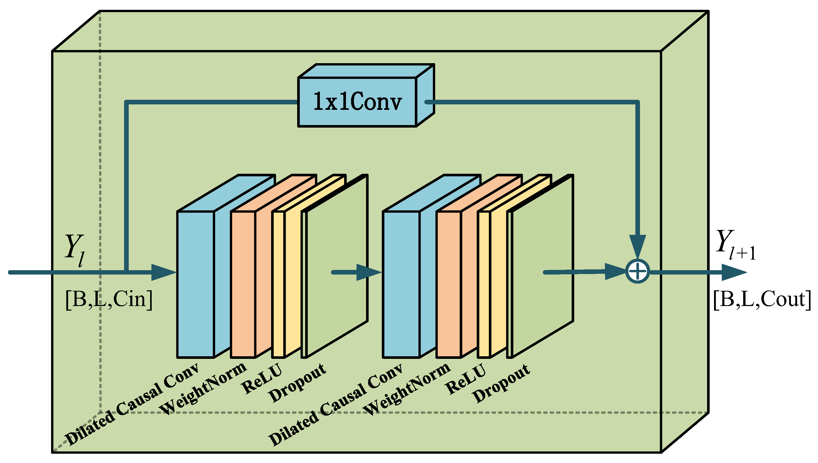
The Temporal Convolutional Network (TCN) is an improved architecture derived from the standard CNN framework, designed to overcome the limitations of traditional recurrent neural networks (such as LSTM) in handling long time-series, including slow training speed and difficulty in capturing long-term dependencies [17]. The core mechanisms of TCNs are causal convolution and dilated convolution, while in practice, the network hierarchy is typically constructed using residual blocks. As illustrated in Figure 3, each residual block consists of two layers of dilated causal convolution, ReLU activation, weight normalization, and dropout. To ensure consistency between the input and output along the channel dimension within the residual connections, a one-dimensional convolution layer is further introduced in the residual path.

During training, the preprocessed data $X\in {\mathbb{R}}^{B\times L\times D}$ is fed into the model. In the TCN, $Y_0\in {\mathbb{R}}^{B\times L\times D}$ denotes the input to the first layer. For any given sample in the batch, its time-series can be expressed as

$$\{y\left(0\right),y\left(1\right),\dots ,y(L-1)\},y\left(t\right)\in {\mathbb{R}}^D$$

(9)

where $y\left(t\right)$ denotes the feature vector at time step t. The TCN produces outputs of the same length as the input sequence. At each time step, the output depends only on the current and previous inputs, thus strictly adhering to causality and preventing information leakage from future time steps.

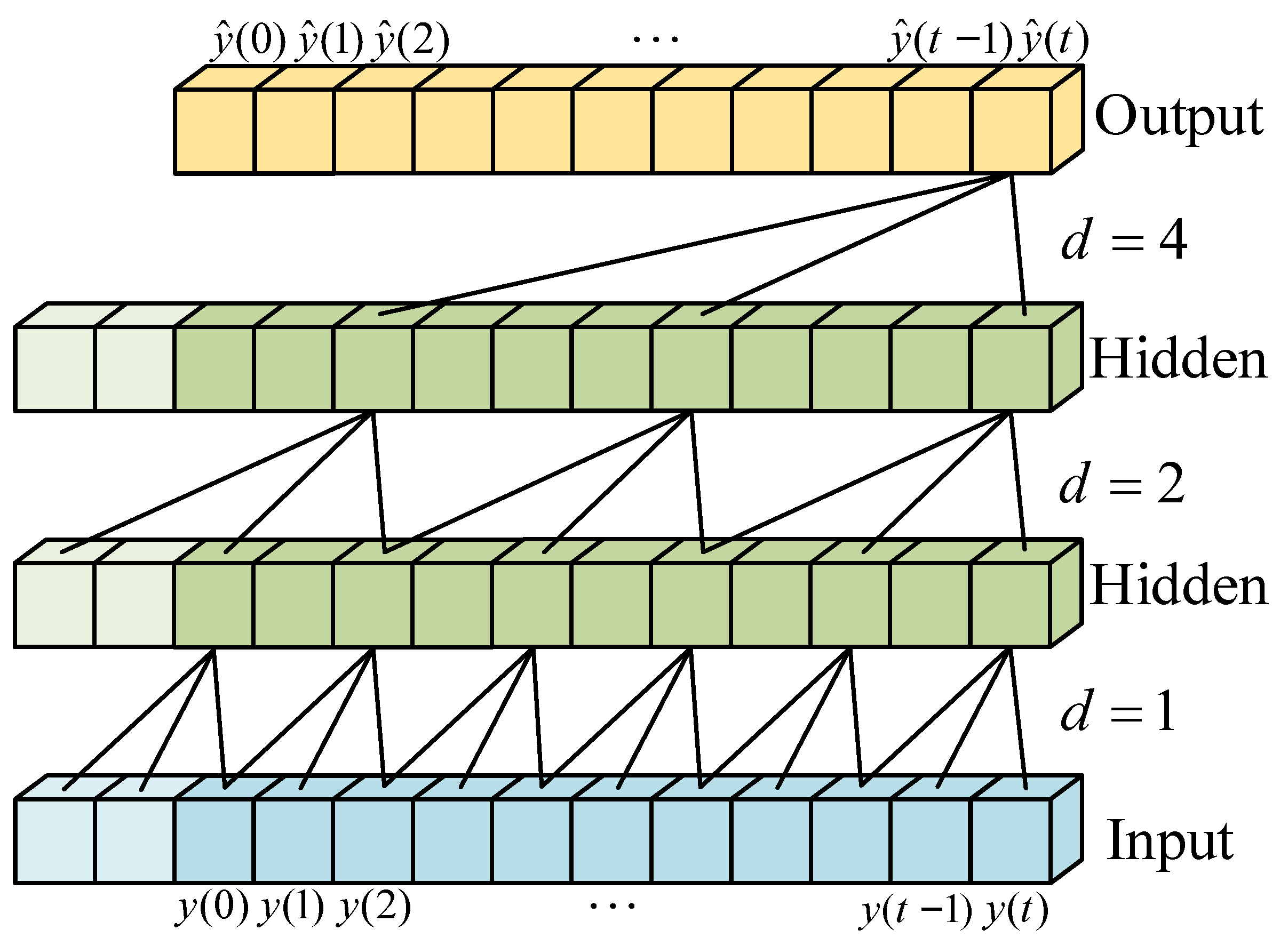
By introducing the dilated convolution mechanism, as illustrated in Figure 4, the receptive field can be rapidly expanded while preserving causality, without a significant increase in model parameters. The computation of multi-channel dilated convolution is formulated as in Equation (10):

$$\widehat{y}\left(t\right)=\sum _{i=0}^{k-1}W\left(i\right)·y(t-d·i)$$

(10)

where k denotes the kernel size, d is the dilation factor, $W\left(i\right)\in {\mathbb{R}}^{C_{\mathrm{out}}\times D}$ represents the weight matrix of the convolution kernel at the i-th position, $y(t-d·i)$ denotes the dilated historical input, and $\widehat{y}\left(t\right)\in {\mathbb{R}}^{C_{\mathrm{out}}}$ denotes the output vector at time step t.

In the TCN component of the proposed TICNet model, three residual blocks are stacked in sequence, with the number of output channels of each block set to $[32,64,128]$. The core structure of a residual block is defined in Equation (11):

$$Y_{l+1}=\sigma \left(\mathrm{ReLU}\left(BN\left(Y_l\ast W_l\right)\right)\right)+\mathrm{Conv}\left(Y_l\right)$$

(11)

where $W_l$ denotes the convolution kernel of the l-th layer, ∗ represents the dilated causal convolution operation, $\sigma$ is the dropout layer, $Y_l\in {\mathbb{R}}^{B\times L\times C_{\mathrm{in}}}$ is the input to the l-th layer, and $Y_{l+1}\in {\mathbb{R}}^{B\times L\times C_{\mathrm{out}}}$ is its output. After the original input $Y_0\in {\mathbb{R}}^{B\times L\times D}$ passes through the three residual blocks, progressively expanding the channel dimension, the final output of the TCN component is $Y_3\in {\mathbb{R}}^{B\times L\times 128}$.

3.2. Informer

Although the self-attention mechanism in conventional Transformers can capture global dependencies, its $O\left(L^2\right)$ time complexity leads to computational bottlenecks in practical long-sequence modeling tasks [22,23,24]. To address this, Informer introduces the ProbSparse self-attention mechanism [25] to reduce computational complexity, and combines it with a feature distillation operation, which progressively filters and compresses redundant information across layers, preserving the most critical global features for the prediction target while maintaining both efficiency and accuracy.

In the proposed TICNet model, only the encoder part of the Informer is employed, retaining two encoder layers and two distillation layers to reduce memory usage and inference latency while maintaining sufficient feature extraction capability. Specifically, the encoder module first maps the input $X\in {\mathbb{R}}^{B\times L\times D}$ to a unified model dimension $d_{model}$ through a linear projection layer; positional encodings are then added to form embeddings with positional information, as shown in Equation (12):

$$X_0=\mathrm{Embedding}\left(X\right)=\mathrm{Linear}\left(X\right)+P{E}_{(L,d_{\mathrm{model}})}\in {\mathbb{R}}^{B\times L\times d_{\mathrm{model}}}$$

(12)

where $PE(·)$ denotes the positional encoding, and the resulting input to the encoder module is $X_0\in {\mathbb{R}}^{B\times L\times d_{mode}}$.

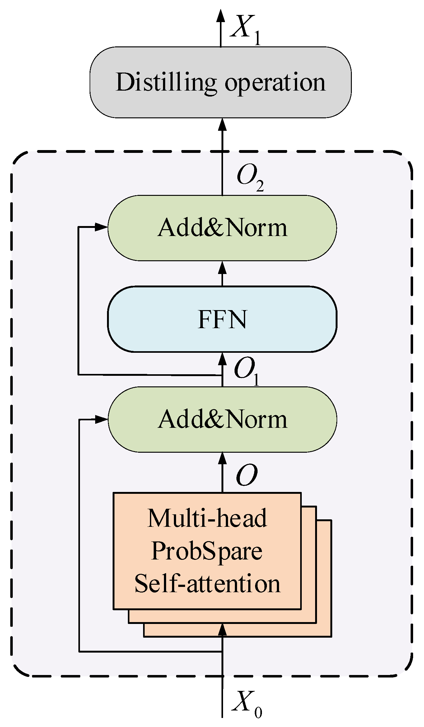
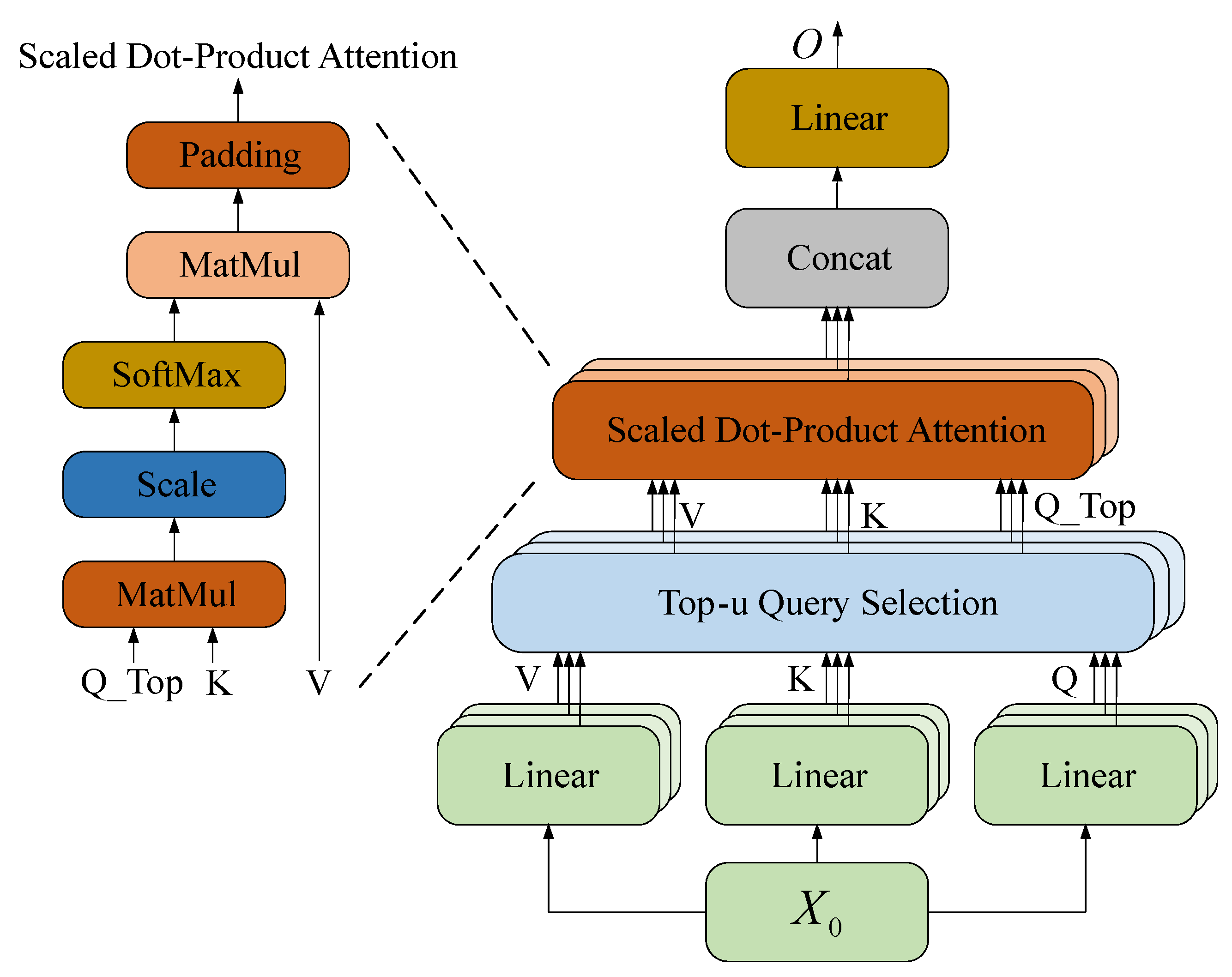
The structure of the encoder layer in the encoder module is illustrated in Figure 5. Each layer primarily consists of a ProbSparse multi-head self-attention mechanism and a feedforward neural network (FNN), with residual connections and layer normalization applied between them to enhance training stability and feature representation capability. The architecture of the ProbSparse self-attention mechanism is shown in Figure 6. Its core idea is as follows: the input sequence $X_0$ is first linearly transformed to obtain the Query, Key, and Value matrices. Through probabilistic selection, only the queries containing the most informative content are retained for attention computation, thereby concentrating computational resources. The corresponding formulation is presented in Equations (13) and (14):

$$Q=X_0{W}_q,K=X_0{W}_k,V=X_0{W}_v$$

(13)

$$M(Q_i,K)=\underset{j}{max}\left({\displaystyle \frac{Q_i·K_j^T}{\sqrt{d}}}\right)-{\displaystyle \frac{1}{L_k}}\sum _{j=1}^{L_k}\left({\displaystyle \frac{Q_i·K_j^T}{\sqrt{d}}}\right)$$

(14)

where, $Q_i$ denotes the i-th Query vector, while $K_j$ and $V_j$ represent the j-th Key and Value vectors, respectively. $W_q$, $W_k$, and $W_v$ are the corresponding weight matrices; $L_k$ is the length of the Key sequence; and d denotes the vector dimension. $max(·)$ refers to the maximum dot product between the Query and all Keys, whereas the latter term represents their arithmetic mean. The metric $M(Q_i,K)$ quantifies how much the maximum attention score of a Query exceeds the mean value. A larger value indicates that the attention distribution is more concentrated, implying greater importance of the corresponding Query.

In practice, only the top $\mathcal{U}$ queries with the highest attention scores are retained for full attention computation, while the remaining queries are approximated using their mean values, thereby reducing the overall computational complexity, as shown in Equation (15):

$$O=\left\{\begin{array}{cc}\sum _{j=1}^{L_k}\mathrm{softmax}\left({\displaystyle \frac{Q_i·K_j^T}{\sqrt{d}}}\right)·V_j,\hfill & i\in \mathcal{U}\hfill \\ \mathrm{mean}\left(V\right),\hfill & i\notin \mathcal{U}\hfill \end{array}\right.$$

(15)

where $O\in {\mathbb{R}}^{B\times L\times d_{mode}}$ denotes the output of the sparse self-attention. This output is processed through a feedforward network with a residual connection, as shown in Equation (16), yielding the output $O_2\in {\mathbb{R}}^{B\times L\times d_{mode}}$ of the encoder layer. After the encoder layer, a distillation operation is applied to compress the sequence length to half of the original, as shown in Equation (17), which preserves the key sequence information while enhancing computational efficiency.

$$\left\{\begin{array}{c}{O}_1=\mathrm{AddNorm}(X_0,O)\hfill \\ O_2=\mathrm{AddNorm}(O_1,\mathrm{FFN}\left(O_1\right))\hfill \end{array}\right.$$

(16)

$$X_1=\mathrm{Distill}\left(O_2\right)=\mathrm{Pool}\left(\mathrm{ReLU}\left(\mathrm{Conv}\left(O_2\right)\right)\right)\in {\mathbb{R}}^{B\times {\displaystyle \frac{L}{2}}\times d_{\mathrm{model}}}$$

(17)

After passing through two encoder layers and corresponding distillation layers, the compressed encoder output $X_2\in {\mathbb{R}}^{B\times {\displaystyle \frac{L}{4}}\times d_{\mathrm{model}}}$ is obtained and serves as the input to the subsequent cross-attention module.

3.3. Cross-Attention Mechanism

The cross-attention mechanism is an attention mechanism designed to model dependencies between two different sequences. Unlike self-attention, which solely captures feature correlations within a single sequence, cross-attention guides one sequence to attend to critical information in another sequence, thereby enabling cross-sequence information alignment and fusion.

Since the output dimensions of the TCN and Informer components differ, they are each projected into the same representation space via linear mappings, as shown in Equation (18):

$$Q_{TCN}=W_Y·Y_3,K_{IF}=W_X·X_2,V_{IF}=W_X·X_2$$

(18)

where $Q_{TCN}$ denotes the output feature map of the TCN component; $W_Y$ is the corresponding weight matrix; $K_{IF}$ and $V_{IF}$ represent the output feature maps of the Informer component; and $W_X$ is the corresponding weight matrix. The information from the two projected channels is normalized via a $softmax$ operation, as shown in Equation (18), to obtain the attention distribution, which is then multiplied with $V_{IF}$ to produce the fused temporal feature $F_{\mathrm{Cross}}\in {\mathbb{R}}^{B\times {\displaystyle \frac{L}{4}}\times 128}$.

Finally, as shown in Equations (19) and (20), the encoded sequence is compressed along the temporal dimension using sequence-wise average pooling to obtain a global representation vector h, which is then fed into a fully connected regression layer to produce the final temperature prediction y.

$$h=\mathrm{MeanPooling}(F_{\mathrm{Cross}},\dim =1),h\in {\mathbb{R}}^{B\times 128}$$

(19)

$$y=\mathrm{FC}\left(h\right),y\in {\mathbb{R}}^{B\times 1}$$

(20)

4. Results

4.1. Experimental Setup and Hyperparameter Settings

The experiments were conducted on a Windows 10 operating system with Python 3.9.21. PyTorch 2.6.0 was used as the deep learning framework, and the computing platform was configured with an Intel Core i7-13700K processor, an NVIDIA GeForce RTX 3080 Ti GPU (with 8 GB of VRAM), 16 GB of RAM, and CUDA 12.7.

A grid search method was employed, and after extensive experiments, the final hyperparameter settings were determined. The hyperparameter values for all models, including TCN-Informer + CrossAttention, are listed in

Table 1. Model parameter settings.

Model Parameters	TCN	Informer Encoder
Number of layers	3	2
Hidden Channels	[32, 64, 128]	\
Number of Attention Heads	\	4
Attention Head Size	\	32
Learning Rate	0.0005	0.0005
Optimizer	Adam	Adam
Activation Function	ReLU	ReLU

. The batch size was set to 32, and the number of training epochs to 100. To mitigate overfitting, Dropout was applied to reduce network complexity and co-adaptation among neurons, with a dropout rate of 0.3.

Mean absolute error ($MAE$), root mean square Error ($RMSE$), and the Coefficient of Determination ($R^2$) were used as evaluation metrics to assess and compare model performance. Their calculation formulas are given in Equations (21)–(23), where n denotes the number of samples, $y_i$ represents the actual temperature value, ${\widehat{y}}_i$ is the predicted value, and ${\overline{y}}_i$ is the mean of all actual values.

$$MAE={\displaystyle \frac{1}{n}}\sum _{i=1}^n\left|y_i-{\widehat{y}}_i\right|$$

(21)

$$RMSE=\sqrt{{\displaystyle \frac{1}{n}}\sum _{i=1}^n{\left(y_i-{\widehat{y}}_i\right)}^2}$$

(22)

$$R^2=1-{\displaystyle \frac{{\sum }_{i=1}^n{\left(y_i-{\widehat{y}}_i\right)}^2}{{\sum }_{i=1}^n{\left(y_i-{\overline{y}}_i\right)}^2}}$$

(23)

4.2. Result Analysis

4.2.1. Model Comparison

To evaluate the performance of the proposed fusion model TICNet in MOSFET temperature prediction, mainstream multivariate time-series prediction models developed in recent years were selected as baselines, including Times-Net, Informer, and LSTM. Specifically, Times-Net is an improved model based on TCNs, Informer is an enhanced model derived from Transformer, and LSTM is a widely used network for addressing long-sequence dependency. All models were trained on the same training set, and their temperature prediction performance was evaluated on the test set.

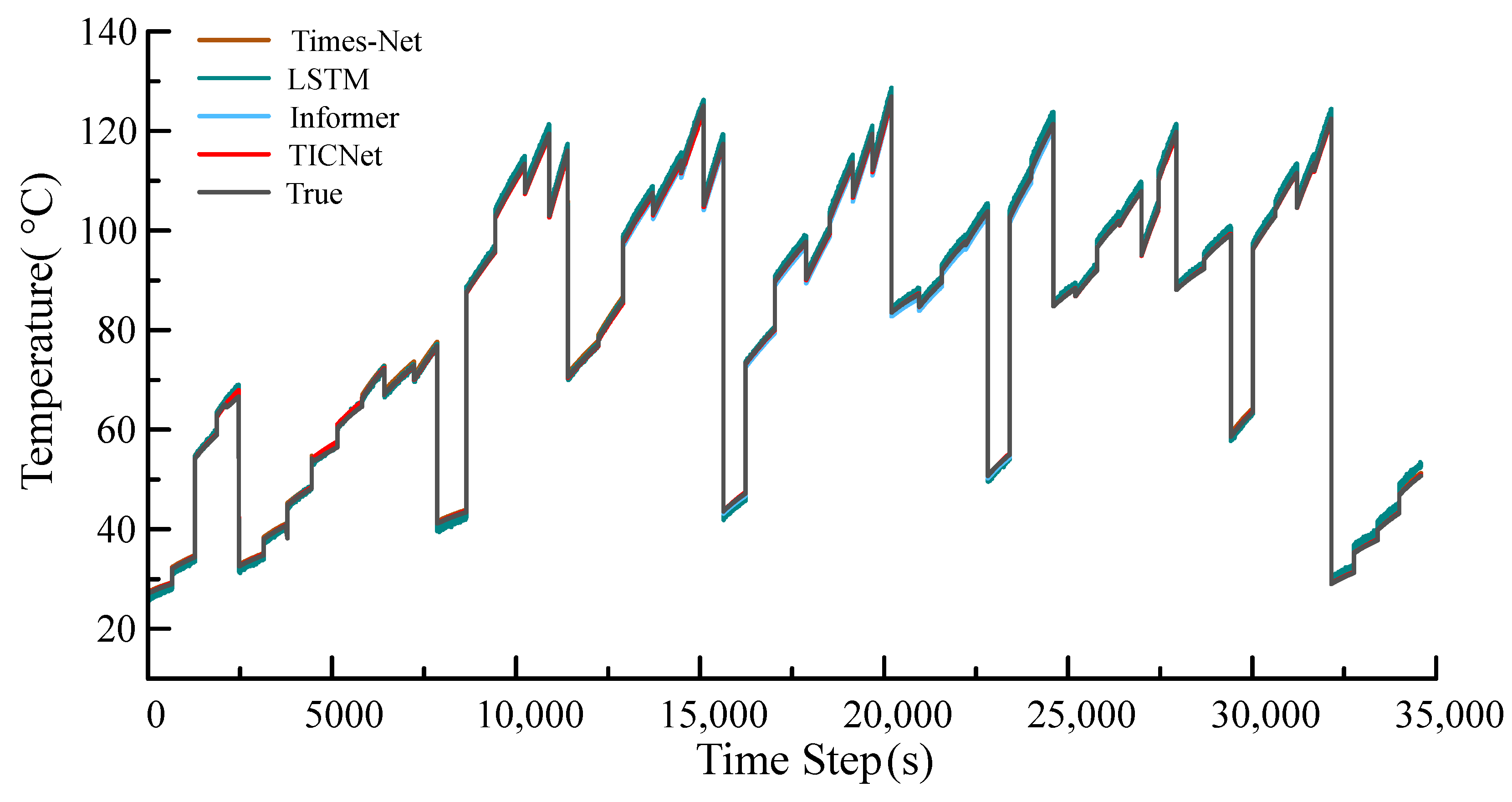
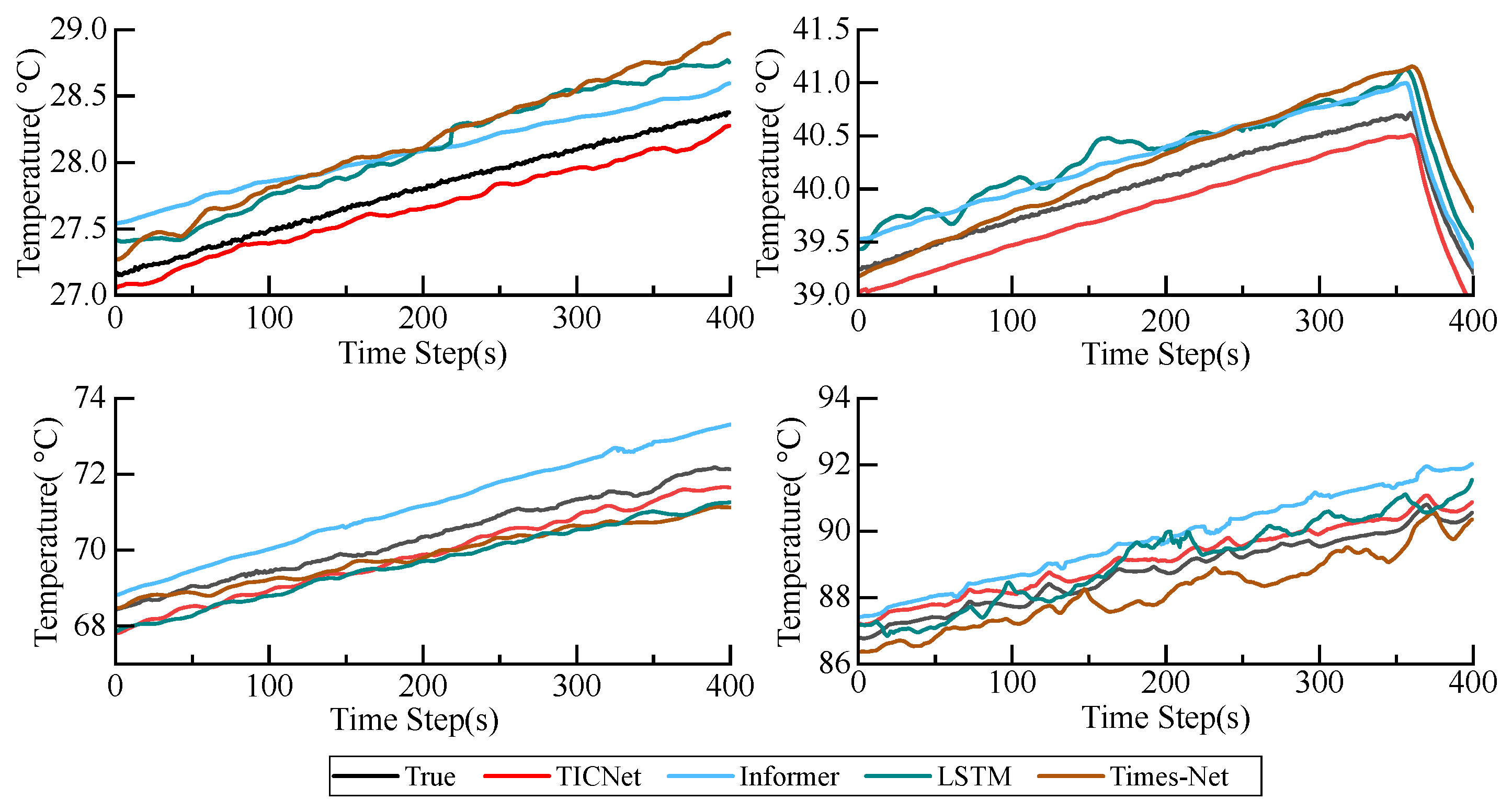
Figure 7 presents the overall prediction results of Times-Net, Informer, LSTM, and the proposed TICNet model on the test set.

Table 2. Overall evaluation metrics.

Model	MAE (°C)	RMSE (°C)	${\mathit{R}}^2$
TICNet	0.2521	0.3641	0.9638
Informer	0.3294	0.4593	0.7436
LSTM	0.9433	1.0853	0.4985
Times-Net	0.4989	0.5753	0.6994

summarizes the overall evaluation metrics of each model on the complete test set. Given the large number of test samples, four typical operating conditions were selected for localized visualization of prediction results, with their specific parameters listed in

Table 3. Parameters of four operating conditions.

Operating Condition	Load Current (A)	Load Voltage (V)	Ambient Temp °C
Condition 1	60	60	0
Condition 2	70	80	20
Condition 3	80	60	40
Condition 4	90	80	60

. The prediction results are shown in Figure 8, where the black curve represents the ground-truth temperature and the red curve corresponds to the prediction of the proposed TICNet model.

Table 4. Performance metrics under typical operating conditions.

Model		TICNet	Informer	LSTM	Times-Net
Condition 1	MAE (°C)	0.1872	0.3114	0.4918	0.4689
	RMSE (°C)	0.2023	0.3257	0.4702	0.4849
	$R^2$	0.9208	0.6565	0.4837	0.2776
Condition 2	MAE (°C)	0.2246	0.3119	0.4495	0.3343
	RMSE (°C)	0.2262	0.3211	0.4556	0.3571
	$R^2$	0.9353	0.7496	0.6493	0.5262
Condition 3	MAE (°C)	0.4647	0.7862	0.9106	0.5974
	RMSE (°C)	0.4702	0.7922	0.9442	0.5838
	$R^2$	0.8998	0.6739	0.3843	0.7055
Condition 4	MAE (°C)	0.3608	0.4288	0.9863	0.6074
	RMSE (°C)	0.3638	0.5119	1.0345	0.6627
	$R^2$	0.8822	0.7667	0.2472	0.6109

further reports the detailed prediction performance of each model under the four typical operating conditions.

As shown in Table 2, the TICNet model significantly outperforms the baseline models in terms of $MAE$, $RMSE$, and $R^2$. Specifically, TICNet records an $MAE$ of $0.2521 °\mathrm{C}$ and an $RMSE$ of $0.3641 °\mathrm{C}$, which are markedly lower than those of LSTM ($0.9433 °\mathrm{C}$/$1.0853 °\mathrm{C}$), Informer ($0.3294 °\mathrm{C}$/$0.4593 °\mathrm{C}$), and Times-Net ($0.4989 °\mathrm{C}$/$0.5753 °\mathrm{C}$). In addition, TICNet attains an $R^2$ of 0.9638, substantially higher than the other models, indicating excellent goodness of fit and predictive accuracy across the full dataset.

Table 4 further shows that TICNet achieves consistent and superior performance across all four operating conditions. Under Condition 1, TICNet yields an $MAE$ of $0.1872 °\mathrm{C}$ and an $RMSE$ of $0.2023 °\mathrm{C}$, with an $R^2$ of 0.9208. Even in the more challenging Condition 4, TICNet still achieves an $MAE$ of $0.3608 °\mathrm{C}$ and an $RMSE$ of $0.3638 °\mathrm{C}$, with an $R^2$ of 0.8822, clearly surpassing the baseline models. These results confirm that TICNet maintains low prediction errors and strong goodness of fit under different operating conditions, demonstrating both stability and generalization capability.

The comparison results also highlight the limitations of the baseline methods. The LSTM model shows larger errors with pronounced fluctuations, confirming its weakness in modeling long-term dependencies and multivariate interactions. The Informer model provides advantages in capturing long-range dependencies but suffers from considerable deviations under complex conditions such as high temperature and high current. The Times-Net model delivers relatively stable performance in some scenarios, yet its overall accuracy remains inferior to TICNet. In contrast, by integrating the local and global temporal feature extraction of the TCN, the long-range dependency modeling of the Informer encoder, and the multi-channel feature fusion enabled by the CrossAttention module, TICNet effectively captures local details, global trends, and cross-feature interactions in MOSFET temperature dynamics, thereby achieving high prediction accuracy under varying load and ambient temperature conditions.

4.2.2. Residual Distribution Analysis

To further illustrate the error distributions of different models under various operating conditions, violin plots of the absolute prediction residuals are presented in Figure 9. As shown, TICNet exhibits noticeably narrower distributions centered at lower values, indicating consistently low and stable prediction errors across all conditions. Under Condition 1 and Condition 2, the errors of TICNet are the most concentrated and skewed toward lower ranges, reflecting high accuracy under stable or moderate-to-low load conditions. Under Condition 3 and Condition 4, although the overall error levels increase, TICNet still maintains a tighter spread with a lower bound, demonstrating superior accuracy and robustness compared with LSTM, Informer, and Times-Net.

In contrast, the LSTM model shows the widest distributions, with errors shifted upward and pronounced long-tail outliers, confirming its vulnerability to large errors in long-sequence and multivariate scenarios. The Informer and Times-Net models present intermediate spreads; however, under high-current or rapid temperature rise conditions, both display wider distributions and higher medians than TICNet, revealing weaker stability in complex scenarios.

The combined analysis of the quantitative results from tables and violin plots confirms that TICNet not only surpasses existing methods in mean error metrics but also shows distinct advantages in the stability and consistency of prediction errors. Overall, TICNet achieves low errors and strong generalization across diverse load and temperature conditions, providing a solid foundation for practical MOSFET temperature prediction under complex operating environments.

4.2.3. Ablation Study

To further investigate the effectiveness of each module in MOSFET temperature prediction, four ablation variants of TICNet were designed by selectively removing or replacing key components. The results are presented in

Table 5. Performance metrics of different model structures.

Model	Component Modules			MAE (°C)	RMSE (°C)	${\mathit{R}}^2$
	TCN	Informer	CrossAttention
TICNet	√	√	√	0.2521	0.3641	0.9638
Structure 1	√	√	×	0.3652	0.3965	0.8925
Structure 2	√	×	√	0.2978	0.3885	0.9341
Structure 3	×	√	×	0.3791	0.4113	0.8708
Structure 4	√	×	×	0.4507	0.4837	0.7644

. When the CrossAttention module was removed and replaced with average fusion, the $MAE$ increased from $0.2521 °\mathrm{C}$ to $0.3652 °\mathrm{C}$, indicating that cross-channel feature fusion facilitates feature coupling and dynamic weighting, thereby enhancing prediction accuracy. Replacing the Informer with a standard Transformer increased the $MAE$ to $0.2978 °\mathrm{C}$, underscoring the importance of long-range dependency modeling and demonstrating the superior accuracy of Informer. Retaining only the single-channel TCN led to a substantial rise in $MAE$ to $0.4507 °\mathrm{C}$, revealing that local and trend features alone are insufficient for high-precision prediction. Conversely, removing the TCN while retaining Informer + CrossAttention yielded an $MAE$ of $0.3791 °\mathrm{C}$—better than standalone TCN but still inferior to the complete TICNet—indicating that long-range dependency modeling and feature fusion cannot fully substitute for TCN’s ability to capture both global trends and local details. Overall, these results validate the synergistic roles of TCN, Informer, and CrossAttention in TICNet, providing strong evidence for achieving accurate and stable MOSFET temperature prediction and supporting its potential for practical engineering applications.

5. Discussion

Taking MOSFET temperature prediction in motor controllers as the research objective, this paper proposes the TICNet model, which integrates the local temporal feature extraction capability of TCNs, the efficient long-range dependency modeling of Informer, and a cross-attention mechanism for multi-feature interaction. TICNet enables accurate prediction of MOSFET temperature under variable operating conditions, effectively overcoming the limitations of traditional methods in prediction accuracy and feature interaction utilization. Experimental results on a real MOSFET temperature dataset show that TICNet achieves an $R^2$ of 0.9638, $MAE$ of $0.2521 °\mathrm{C}$ and $RMSE$ of $0.3641 °\mathrm{C}$. Compared with existing methods such as Times-Net, Informer, and LSTM, TICNet reduces $MAE$ by 0.0773–$0.6912 °\mathrm{C}$ and $RMSE$ by 0.0952–$0.7212 °\mathrm{C}$. These results demonstrate superior accuracy and generalization for multivariate time-series prediction, highlighting its potential for practical engineering applications. Future work will focus on further optimizing the model structure and integrating it with embedded deployment to enable real-time online temperature prediction.

References

1. Huang, Q.; Huang, Q.; Guo, H.; Cao, J. Design and research of permanent magnet synchronous motor controller for electric vehicle. Energy Sci. Eng. 2023, 11, 112–126. [Google Scholar] [CrossRef]
2. Shu, X.; Guo, Y.; Yang, H.; Zou, H.; Wei, K. Reliability study of motor controller in electric vehicle by the approach of fault tree analysis. Eng. Fail. Anal. 2021, 121, 105165. [Google Scholar] [CrossRef]
3. Vankayalapati, B.T.; Sajadi, R.; Cn, M.A.; Deshmukh, A.V.; Farhadi, M.; Akin, B. Model based junction temperature profile control of SiC MOSFETs in DC power cycling for accurate reliability assessments. IEEE Trans. Ind. Appl. 2024, 60, 7216–7224. [Google Scholar] [CrossRef]
4. Lai, W.; Wei, Y.; Chen, M.; Xia, H.; Luo, D.; Li, H. In-situ calibration method of online junction temperature estimation in IGBTs for electric vehicle drives. IEEE Trans. Power Electron. 2022, 38, 1178–1189. [Google Scholar] [CrossRef]
5. Ma, M.; Sun, Z.; Wang, Y.; Wang, J.; Wang, R. Method of junction temperature estimation and over temperature protection used for electric vehicle’s IGBT power modules. Microelectron. Reliab. 2018, 88, 1226–1230. [Google Scholar] [CrossRef]
6. Yang, Y.; Wu, Y.; Ding, X.; Zhang, P. Online junction temperature estimation method for SiC MOSFETs based on the DC bus voltage undershoot. IEEE Trans. Power Electron. 2023, 38, 5422–5431. [Google Scholar] [CrossRef]
7. Li, C.; Lu, Z.; Wu, H.; Li, W.; He, X.; Li, S. Junction temperature measurement based on electroluminescence effect in body diode of SiC power MOSFET. In Proceedings of the 2019 IEEE Applied Power Electronics Conference and Exposition (APEC), Anaheim, CA, USA, 17–21 March 2019; IEEE: Piscataway, NJ, USA, 2019; pp. 338–343. [Google Scholar]
8. Lee, I.H.; Lee, K.B. Junction temperature estimation of SiC MOSFETs in three-level NPC inverters. J. Electr. Eng. Technol. 2024, 19, 1607–1617. [Google Scholar] [CrossRef]
9. Meng, X.; Zhang, M.; Feng, S.; Tang, Y.; Zhang, Y. Online temperature measurement method for SiC MOSFET device based on gate pulse. IEEE Trans. Power Electron. 2024, 39, 4714–4724. [Google Scholar] [CrossRef]
10. Teixeira, A.; Cougo, B.; Segond, G.; Morais, L.M.F.; Andrade, M.; Tran, D.H. Precise estimation of dynamic junction temperature of SiC transistors for lifetime prediction of power modules used in three-phase inverters. Microelectron. Reliab. 2023, 150, 115137. [Google Scholar] [CrossRef]
11. Matallana, A.; Robles, E.; Ibarra, E.; Andreu, J.; Delmonte, N.; Cova, P. A methodology to determine reliability issues in automotive SiC power modules combining 1D and 3D thermal simulations under driving cycle profiles. Microelectron. Reliab. 2019, 102, 113500. [Google Scholar] [CrossRef]
12. Eleffendi, M.A.; Johnson, C.M. Application of Kalman filter to estimate junction temperature in IGBT power modules. IEEE Trans. Power Electron. 2016, 31, 1576–1587. [Google Scholar] [CrossRef]
13. Miao, J.; Yin, Q.; Wang, H.; Liu, Y.; Li, H.; Duan, S. IGBT junction temperature estimation based on machine learning method. In Proceedings of the 2020 IEEE 9th International Power Electronics and Motion Control Conference (IPEMC2020-ECCE Asia), Nanjing, China, 29 November–2 December 2020; IEEE: Piscataway, NJ, USA, 2020; pp. 1–5. [Google Scholar]
14. Kim, M.K.; Yoon, Y.D.; Yoon, S.W. Actual maximum junction temperature estimation process of multichip SiC MOSFET power modules with new calibration method and deep learning. IEEE J. Emerg. Sel. Top. Power Electron. 2023, 11, 5602–5612. [Google Scholar] [CrossRef]
15. Shuai, Z.; He, S.; Xue, Y.; Zheng, Y.; Gai, J.; Li, Y.; Li, G.; Li, J. Junction temperature estimation of a SiC MOSFET module for 800 V high-voltage application in electric vehicles. eTransportation 2023, 16, 100241. [Google Scholar] [CrossRef]
16. Du, Z.W.; Zhang, Y.; Wang, Y.; Chen, Z.; Wang, Y.-D.; Wu, R.; Zhao, D.; Zhang, X.; Yin, W.-Y. A time series characterization of IGBT junction temperature method based on LSTM network. IEEE Trans. Power Electron. 2025, 40, 2070–2085. [Google Scholar] [CrossRef]
17. Bai, S.J.; Kolter, J.Z.; Koltun, V. An empirical evaluation of generic convolutional and recurrent networks for sequence modeling. arXiv 2018, arXiv:1803.01271. [Google Scholar] [CrossRef]
18. Chen, Z.L.; Ma, M.B.; Li, T.R.; Wang, H.J.; Li, C.S. Long sequence time-series forecasting with deep learning: A survey. Inf. Fusion 2023, 97, 101819. [Google Scholar] [CrossRef]
19. Liu, X.; Wang, W. Deep time series forecasting models: A comprehensive survey. Mathematics 2024, 12, 1504. [Google Scholar] [CrossRef]
20. Lim, H.; Hwang, J.; Kwon, S.; Baek, H.; Uhm, J.; Lee, G. A study on real time IGBT junction temperature estimation using the NTC and calculation of power losses in the automotive inverter system. Sensors 2021, 21, 2454. [Google Scholar] [CrossRef] [PubMed]
21. Ding, X.F.; Lu, P.; Shan, Z.Y. A high-accuracy switching loss model of SiC MOSFETs in a motor drive for electric vehicles. Appl. Energy 2021, 291, 116827. [Google Scholar] [CrossRef]
22. Vaswani, A.; Shazeer, N.; Parmar, N.; Uszkoreit, J.; Jones, L.; Gomez, A.N.; Kaiser, Ł.; Polosukhin, I. Attention is all you need. In Proceedings of the 31st International Conference on Neural Information Processing Systems (NIPS’17), Long Beach, CA, USA, 4–9 December 2017; Curran Associates Inc.: Red Hook, NY, USA, 2017; pp. 6000–6010. [Google Scholar]
23. Bahdanau, D.; Cho, K.; Bengio, Y. Neural machine translation by jointly learning to align and translate. arXiv 2014, arXiv:1409.0473. [Google Scholar]
24. Zhang, Y.; Yan, J. Crossformer: Transformer utilizing cross-dimension dependency for multivariate time series forecasting. In Proceedings of the Eleventh International Conference on Learning Representations, Kigali, Rwanda, 1–5 May 2023. [Google Scholar]
25. Zhou, H.; Zhang, S.; Peng, J.; Zhang, S.; Li, J.; Xiong, H.; Zhang, W. Informer: Beyond efficient transformer for long sequence time-series forecasting. In Proceedings of the AAAI Conference on Artificial Intelligence, Virtual, 19–21 May 2021; Volume 35, pp. 11106–11115. [Google Scholar]
Figure 1. Simplified diagram of the three-phase inverter circuit in the motor controller.
Information 16 00872 g001
Figure 2. Overall architecture of the model.
Information 16 00872 g002
Figure 3. Structure of the TCN residual block.
Information 16 00872 g003
Figure 4. Dilated causal convolution.
Information 16 00872 g004
Figure 5. Encoder layer structure.
Information 16 00872 g005
Figure 6. Multi-head ProbSpare self-attention.
Information 16 00872 g006
Figure 7. Overall prediction comparison results.
Information 16 00872 g007
Figure 8. Local prediction comparison results.
Information 16 00872 g008
Figure 9. Residual comparison results.
Information 16 00872 g009