Article

Explainable Instrument Classification: From MFCC Mean-Vector Models to CNNs on MFCC and Mel-Spectrograms with t-SNE and Grad-CAM Insights

Department of Civil, Computer Science and Aeronautical Technologies Engineering, Università degli Studi Roma Tre, Via V. Volterra 62, 00146 Roma, Italy
*
Author to whom correspondence should be addressed.
Information 2025, 16(10), 864; https://doi.org/10.3390/info16100864
Submission received: 26 August 2025 / Revised: 24 September 2025 / Accepted: 3 October 2025 / Published: 5 October 2025
(This article belongs to the Special Issue Artificial Intelligence for Acoustics and Audio Signal Processing)

Abstract

This paper presents an automatic system for the classification of musical instruments from audio recordings. The project leverages deep learning (DL) techniques to achieve its objective, exploring three different classification approaches based on distinct input representations. The first method involves the extraction of Mel-Frequency Cepstral Coefficients (MFCCs) from the audio files, which are then fed into a two-dimensional convolutional neural network (Conv2D). The second approach makes use of mel-spectrogram images as input to a similar Conv2D architecture. The third approach employs conventional machine learning (ML) classifiers, including Logistic Regression, K-Nearest Neighbors, and Random Forest, trained on MFCC-derived feature vectors. To gain insight into the behavior of the DL model, explainability techniques were applied to the Conv2D model using mel-spectrograms, allowing for a better understanding of how the network interprets relevant features for classification. Additionally, t-distributed stochastic neighbor embedding (t-SNE) was employed on the MFCC vectors to visualize how instrument classes are organized in the feature space. One of the main challenges encountered was the class imbalance within the dataset, which was addressed by assigning class-specific weights during training. The results, in terms of classification accuracy, were very satisfactory across all approaches, with the convolutional models and Random Forest achieving around 97–98%, and Logistic Regression yielding slightly lower performance. In conclusion, the proposed methods proved effective for the selected dataset, and future work may focus on further improving class balance techniques.

1. Introduction

The analysis of audio signals remains a significant and ongoing challenge in the field of signal processing and data interpretation, largely due to the intrinsic characteristics of audio data. These signals are typically non-stationary, high-dimensional, and highly sensitive to noise and contextual variability, which complicates their analysis and demands sophisticated processing techniques. Traditional methods, such as Fourier analysis, have proven to be fundamental tools in this domain. By transforming time-domain signals into the frequency domain, these methods enable the extraction of informative features that reveal the underlying spectral structure of audio content. This transformation supports a wide range of tasks, including classification, enhancement, segmentation, and anomaly detection [1,2,3].
With the advent of artificial intelligence (AI), and in particular deep learning, a data-driven paradigm has emerged that minimizes the need for manual feature engineering. Neural networks, especially convolutional and recurrent architectures, are capable of learning complex patterns directly from raw or minimally processed audio [4,5,6,7]. However, to fully leverage the capabilities of AI models, it is critical to provide them with structured and informative input data. This is where the integration of traditional signal processing with deep learning becomes essential. Time-frequency representations, such as spectrograms and mel-spectrograms, preserve both temporal and spectral information, enabling neural networks to more effectively learn discriminative features relevant to audio classification tasks [8,9].
One prominent application of these techniques is automatic musical instrument classification, a core problem in the field of Music Information Retrieval (MIR) [10]. Accurately identifying the instrument from an audio signal is inherently complex due to variations in timbre, playing techniques, recording conditions, and the presence of overlapping sources. While traditional classifiers based on hand-crafted features offer limited performance, modern approaches increasingly rely on convolutional neural networks (CNNs) trained on time-frequency representations. These models have shown substantial improvements in recognizing instrument characteristics and adapting to diverse acoustic contexts.
However, as deep learning models grow in complexity, they also become more opaque—posing challenges in terms of interpretability and explainability. Understanding the methods and the reasons why a model arrives at a particular decision is crucial, especially in domains where reliability and transparency are paramount. In the context of audio signal classification, explainability helps researchers and practitioners assess model behavior, diagnose errors, detect biases, and ultimately build more trustworthy systems [11,12,13,14].
The objective of this work is to contribute to this intersection between deep learning, signal processing, and explainable AI. By leveraging time-frequency feature extraction and applying interpretable deep learning models to the task of musical instrument recognition, the goal is not only to achieve high classification performance but also to provide insights into the decision-making process of these models. The explainability techniques are key to validating the reliability of AI systems and ensuring their applicability in real-world music-related tasks, including education, recommendation, and automated audio tagging. The structure of this paper is as follows:
  • Section 2 reviews related works on musical instrument classification and the main techniques employed in the literature;
  • Section 3 presents the materials and methods, including dataset preparation, feature extraction, and the architecture of the neural models used;
  • Section 4 reports the experimental results and evaluation metrics, with particular focus on the explainability techniques adopted to interpret model behavior;
  • Section 5, finally, provides conclusions and discusses possible future developments.

2. Related Works

Automatic analysis and classification of musical instrument signals has progressed for more than three decades, moving from hand-crafted descriptors and shallow classifiers to end-to-end deep-learning architectures.

2.1. Early Feature-Based Pipelines (1990–2000)

Kaminskyj & Materka pioneered energy-envelope features plus k-nearest-neighbor (k-NN), already distinguishing four monophonic instruments with 98% accuracy [15]. Brown then demonstrated the effectiveness of Mel-frequency cepstral coefficients (MFCCs), reporting 80% accuracy over fifteen orchestral instruments and 94% at the family level [16]. Marques & Moreno introduced Gaussian Mixture Models (GMMs) and Support Vector Machines (SVMs), cutting the error rate on eight instruments to 17% for 2-s excerpts [17].

2.2. First Wave of Large-Scale Studies (2000–2006)

Eronen & Klapuri combined cepstral, spectral-shape, and temporal-envelope features, reaching 94% accuracy at family level on 30 instruments [18]. Kostek & Czyżewski fused MPEG-7 descriptors with wavelet coefficients and a shallow neural network, achieving 94.5% accuracy on 12 studio-recorded instruments [19]. Livshin & Rodet showed that single-database evaluations overestimate performance: accuracy dropped from 90% to 60% when models were tested cross-database [20]. Agostini et al. evaluated compact spectral descriptors: centroid, inharmonicity, and first-partial energy and found Quadratic Discriminant Analysis superior to k-NN on 27 instruments [21]. Krishna & Sreenivas extended recognition from isolated notes to solo phrases with Line Spectral Frequencies (LSF) and GMMs, retaining 77% accuracy on phrases [22]. Essid, Richard & David introduced pairwise feature selection with one-vs-one SVMs, surpassing 93% on 11 solo instruments [23].

2.3. New Descriptors and Unsupervised Codes (2010–2014)

Diment et al. exploited phase information via the Modified Group-Delay Function (MODGD), improving MFCC baselines by +5% on 22 instruments [24]. Yu et al. learned sparse cepstral codes with dictionary learning, pushing single-note recognition to 96% on 50 instruments and a 66% F-measure in mixture tests [25].

2.4. Deep-Learning Era (2016–2024)

Polyphonic milestone. Han, Kim & Lee applied a deep convolutional neural network (CNN) to polyphonic music (IRMAS), boosting micro-F1 to 0.60 without explicit source separation [26].
End-to-end audio. Lee et al. showed that sample-level 1-D CNNs fed with raw waveforms rival log-Mel models, reaching AUC ≈ 0.91 on instrument tags [27].
CNN refinements. Haidar-Ahmad proposed a 4-class CNN yielding 70% precision on dominant-instrument tags [28]. Gururani, Sharma & Lerch embedded frame-wise attention in a CRNN, gaining +3–5 pp Average Precision on OpenMIC [29].
Modern CNN variants (2022). Solanki & Pandey designed an 8-layer CNN that reached 92.8% accuracy on real-world polyphonic excerpts [30]. Blaszke & Kostek introduced per-instrument CNN specialists, achieving precision from 0.86 (guitar) to 0.99 (drums) [31].
Transformers and ensembles. Reghunath & Rajan fused Vision- and Swin-Transformers over Mel-spectrogram, MODGD-gram, and tempogram views, raising IRMAS micro-F1 to 0.66 [32].
Interpretability. Chen et al. analyzed CNN attention with CAM/IG heat maps on six spectral representations on NSynth, confirming MFCC and logMel as the most informative while highlighting complementary cues from Chroma and Tonnetz [33].
Over time, musical instrument recognition has evolved from handcrafted features and shallow classifiers to fully data-driven models such as CNNs and Transformer ensembles. While near-perfect accuracy is attainable on isolated notes, robust recognition in real-world polyphony remains challenging, although recent Transformer hybrids significantly narrow the gap.
In the next section, we build upon this background to present our dataset, features, and modeling approach.

3. Materials and Methods

3.1. Dataset

The dataset used in this study is the Music Instrument Sounds for Classification dataset (https://www.kaggle.com/datasets/abdulvahap/music-instrunment-sounds-for-classification, accessed on 1 October 2025), publicly available on Kaggle. This dataset was selected due to its comprehensive coverage of 28 distinct instrument classes, which provides a robust and wide-ranging benchmark for evaluating diverse feature representations and classification methodologies. The broad class distribution is essential for assessing model generalizability and performance across a large number of instrument timbres. Furthermore, the standardized structure and high-quality recordings provide a controlled environment, which is critical for ensuring reproducibility and direct comparability of results across different research efforts. The integrity and standardized format of the data are prerequisites for developing and validating robust methodologies before their application to more complex, real-world acoustic scenarios. It has been specifically curated to support research in audio signal processing, machine learning, and music information retrieval. The dataset consists of high-quality .wav recordings, each capturing a clear and isolated performance with minimal background noise. This makes the dataset particularly suitable for supervised learning tasks such as instrument classification and recognition.
To ensure temporal consistency and facilitate batch processing during model training, all audio samples were standardized to a fixed duration of three seconds. Recordings that contained extended silences or exhibited poor audio quality were excluded, thereby improving the overall integrity and relevance of the dataset. The audio clips are formatted in the .wav format, which is widely compatible with standard audio processing libraries such as Librosa.
The dataset covers a wide range of instrument families, including strings, winds, keyboards, and percussions. The instruments analyzed in this study are the accordion, acoustic guitar, banjo, bass guitar, clarinet, cowbell, cymbals, dobro, drum set, electric guitar, floor tom, flute, harmonica, harmonium, hi-hats, horn, keyboard, mandolin, organ, piano, saxophone, shakers, tambourine, trombone, trumpet, ukulele, vibraphone, and violin. A significant characteristic of the dataset is the imbalance in the number of samples per instrument class: certain instruments, such as the acoustic guitar, flute, and drum set, are represented by several thousand samples, while others, including the harmonica, cymbals, and saxophone, have considerably fewer examples. This uneven distribution poses a challenge for model training, as it can lead to biased learning outcomes favoring the more frequent classes.
To provide a clearer understanding of the dataset composition, Figure 1 presents a bar plot that visually conveys the number of samples available for each instrument. This visualization highlights the extent of the class imbalance and helps inform preprocessing and modeling decisions.

3.2. Libraries

For the processing of audio data, extensive use was made of Python’s scientific libraries. Among them, Librosa (version 0.11.0) played a central role, proving to be an essential tool for audio analysis and feature extraction.
Librosa is an open-source Python library (Python 3.13.7) specifically designed for audio signal analysis and processing, with a strong focus on machine learning and deep learning applications. It supports various audio formats such as WAV, MP3, and FLAC, and provides a comprehensive set of tools for extracting audio features, including MFCCs, spectrograms, chromagrams, tempo, pitch, and more [34].
Beyond feature extraction, Librosa offers advanced functionality for audio visualization and manipulation, such as Fourier transforms, spectrogram generation, beat tracking, harmonic-percussive source separation, pitch shifting, time stretching, and structural analysis of audio tracks.
Thanks to its intuitive API and seamless integration with visualization libraries like Matplotlib (version 3.10), Librosa stands out as a highly versatile and indispensable tool in music classification, speech recognition, and audio signal processing projects.
In this project, extensive use was also made of Keras for implementing and training the neural network models. Keras is an open-source Python library for deep learning, designed to streamline the development, training, and evaluation of neural networks: it allows the integration of custom layers, activation functions, loss functions, and optimizers, making it adaptable to a wide range of projects. Keras is compatible with several computational backends, including TensorFlow, Theano, and Microsoft Cognitive Toolkit (CNTK), and can run on CPUs, GPUs, and TPUs.

3.3. Data Analysis

In the initial phase, an exploratory analysis of the dataset was carried out to understand its structure and to examine the characteristics of the instances with respect to the different musical instrument classes.
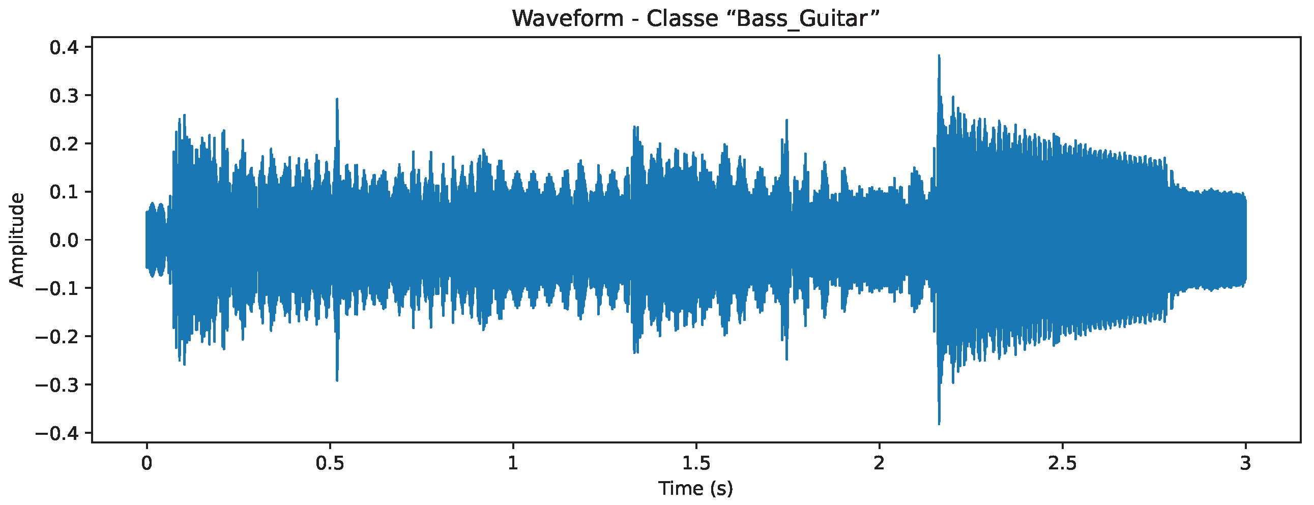
The distribution of audio files per class was then analyzed: as shown in Figure 1, the dataset is significantly unbalanced, with the number of samples varying considerably across classes, as previously discussed. This class imbalance issue will be addressed during the training phase of the deep learning model, using specific techniques aimed at mitigating the impact of unequal class representation. Subsequently, the analysis was deepened through the visualization of waveforms as shown in Figure 2. Waveforms provide a graphical representation of an audio signal in the time domain, enabling the analysis of amplitude variations over time. The horizontal axis represents time progression, while the vertical axis indicates the amplitude of the signal, which corresponds to sound intensity at a given moment. A higher amplitude reflects a louder sound, whereas a lower amplitude indicates a softer one. This visual representation serves as a fundamental tool for audio analysis: examining a waveform allows for the identification of pauses and silent segments, assessment of intensity fluctuations, and recognition of distinctive patterns.

3.4. Data Pre-Processing

The data preprocessing procedure was divided into two distinct phases: feature extraction and standardization.

3.5. Mel Spectrogram and Mel-Frequency Cepstral Coefficients (MFCCs)

Mel-Frequency Cepstral Coefficients (MFCCs) and Mel spectrograms are widely used feature representations in audio signal processing, particularly in applications such as speech recognition, music classification, and instrument identification. Both techniques aim to model audio in a way that closely aligns with human auditory perception.
Mel-Frequency Cepstral Coefficients (MFCCs) provide a compact representation of the spectral characteristics of an audio signal over short time frames, effectively capturing the timbral and tonal attributes of the sound. The computation begins by dividing the audio signal x [ n ] into overlapping frames, typically 20–40 ms long, to ensure local stationarity. A window function w [ n ] , such as a Hamming window, is applied to each frame to minimize spectral leakage [6,35].
Next, the Fourier Transform is computed to extract the frequency spectrum of each frame. This is given by the Short-Time Fourier Transform (STFT):
X ( k ) = n = 0 N 1 x ( n ) · w ( n ) · e j 2 π k n / N
The magnitude spectrum is then converted into a power spectrum:
P ( k ) = | X ( k ) | 2
To better reflect human auditory sensitivity to different frequency bands, the power spectrum is passed through a Mel filter bank, which are triangular filters spaced according to the Mel scale: this scale provides higher resolution at lower frequencies and compression at higher frequencies, mimicking the human ear’s nonlinear perception of pitch. The Mel filter bank is defined as:
M ( f ) = 2595 · log 10 1 + f 700
The output of each Mel filter is then passed through a logarithmic function to approximate the nonlinear sensitivity of human hearing:
log E m = log k = 1 K P [ k ] · H m [ k ]
where H m [ k ] denotes the response of the m–th Mel filter.
Finally, the Discrete Cosine Transform (DCT) is applied to the log filterbank energies to decorrelate the coefficients and reduce dimensionality:
MFCC n = m = 1 M log E m · cos π n M m 1 2
The resulting MFCCs effectively capture the timbral and tonal attributes of the sound and are particularly useful for distinguishing between different musical instruments or phonetic elements.
The Mel spectrogram is a time-frequency representation of audio that incorporates the Mel scale to align with the nonlinear frequency sensitivity of human auditory perception. Similarly to a traditional spectrogram, it displays the temporal evolution of spectral energy, with time represented on the horizontal axis and frequency on the vertical axis. However, unlike the linear frequency scale used in conventional spectrograms, the Mel spectrogram employs a perceptual scale that emphasizes lower frequencies while compressing higher frequencies. This transformation enhances the representation of features most relevant to human hearing [36].
To compute a Mel spectrogram, the short-time Fourier transform (STFT) is first applied to the audio signal to obtain the power spectrogram, denoted as | X [ k , t ] | 2 , where k and t correspond to frequency and time indices, respectively. A bank of triangular filters spaced according to the Mel scale is then applied to the power spectrum to produce the Mel-frequency spectrogram:
S ( m , t ) = k = 1 K | X ( k , t ) | 2 · H m ( k )
where, again, H m [ k ] represents the m–th Mel filter.
Then, an optional logarithmic transformation is often performed for dynamic range compression and to approximate the human perception of loudness.
The resulting two-dimensional matrix can be visualized as a heatmap, where the intensity of each time-frequency bin reflects the signal’s energy content. This representation effectively captures perceptually salient audio features such as harmonic structure, timbre, and transient events. Due to its robustness and alignment with human hearing, the Mel spectrogram is widely utilized in tasks such as speech recognition, music information retrieval, and audio classification. Figure 3 shows an example of a Mel spectrogram representation.

3.5.1. Features Extraction

In the first phase, audio data were initially loaded using the .load module from the Librosa library, followed by the extraction of relevant features. During this process, it was observed that performing loading and feature extraction simultaneously resulted in significant computational delays. Consequently, the two steps were separated: all audio files were pre-loaded using Librosa, and feature extraction was then executed in parallel, leveraging all available CPU cores (22 cores in this case). This modification led to a substantial improvement in processing time, reducing the combined loading and extraction time from approximately 10 min to roughly 4 min for loading and 1 min for extraction.
Specifically, Mel-Frequency Cepstral Coefficients (MFCCs) and Mel spectrograms were extracted and used to train two separate models.

3.5.2. Standardization

The second phase involved standardizing the extracted features to bring their numerical values onto comparable scales, thereby enhancing the stability and efficiency of model training. StandardScaler from common libraries could not be used, as it operates on 2D arrays while the data were structured as 3D arrays. Therefore, a custom standardization function was implemented to normalize only the last two dimensions of the array by computing their mean and standard deviation.

3.6. CNN-Based Models

Before model construction, the preprocessed data were randomly shuffled and split into training, validation, and test sets with an 80-10-10 ratio using a stratified sampling strategy. This ensures that the class proportions are preserved across all splits, thereby maintaining consistency in the representation of both frequent and rare instruments. Stratification is particularly important in the presence of class imbalance, as it prevents underrepresented classes from being excluded from the validation or test sets. To guarantee reproducibility of the experiments, the entire splitting procedure was performed with a fixed random seed (22). The label vector, initially categorical, was transformed into binary numerical vectors through one-hot encoding.
Additionally, a new dimension was added to the data arrays to match the input shape required by the neural network.

3.6.1. Model Construction

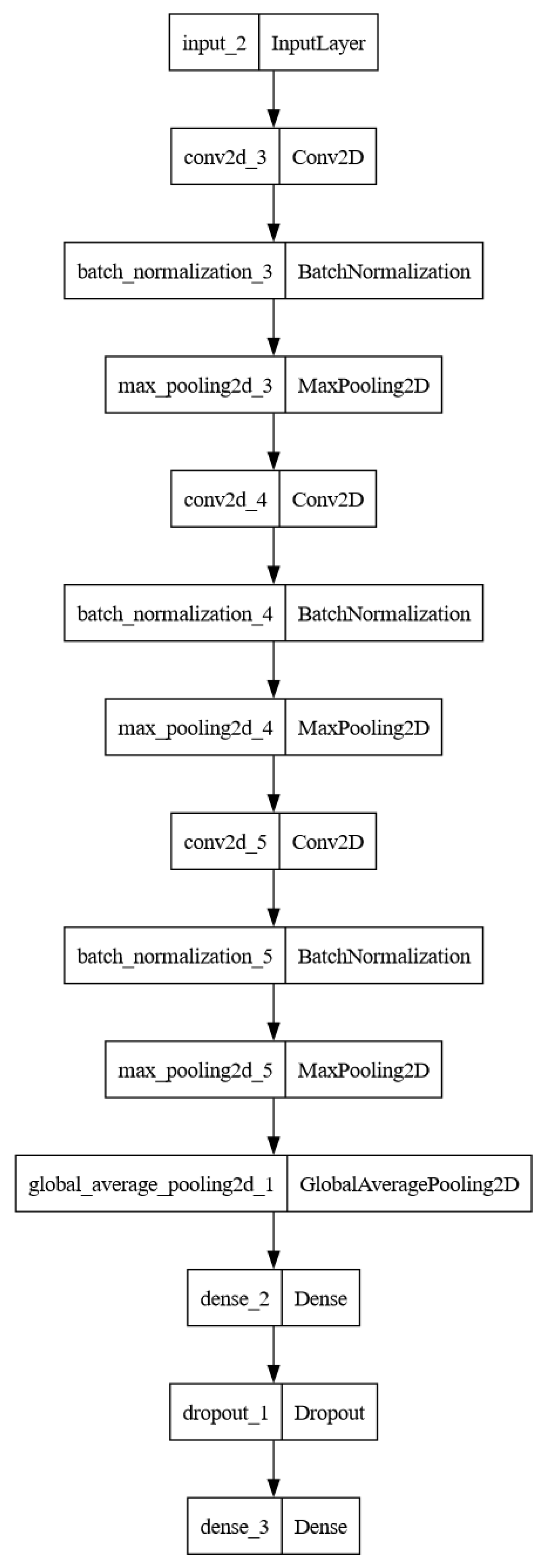
In this study, a two-dimensional convolutional neural network (2D CNN) was implemented for multi-class classification. For an effective understanding of the proposed architecture, a schematic representation is provided in Figure 4.
The architecture follows a typical hierarchical CNN structure and incorporates batch normalization to enhance numerical stability and accelerate training convergence. The model consists of three convolutional blocks, each comprising a Conv2D layer with kernel size 3 × 3, ReLU activation, and “same” padding, followed by a BatchNormalization layer and a MaxPooling2D layer with pool size 2 × 2. These blocks use 32, 64, and 128 filters, respectively, enabling the extraction of progressively more abstract and complex features.
Following the convolutional layers, a GlobalAveragePooling2D layer was added to reduce the feature maps into a one-dimensional vector. This step reduces the number of trainable parameters and helps mitigate overfitting.
A fully connected dense layer with 128 ReLU-activated units was then applied, followed by a dropout layer with a dropout rate of 0.5 to promote model generalization by introducing noise during training.
The output layer is a dense layer with softmax activation and a number of units equal to the number of target classes, producing a probability distribution across the label space.

3.6.2. Training

The model was compiled using the Adam optimizer with an initial learning rate of 0.001, and categorical cross-entropy was employed as the loss function, which is suitable for multi-class classification tasks with one-hot encoded labels. Accuracy was used as the evaluation metric during training.
To prevent overfitting, an early stopping mechanism was employed, monitoring the validation loss and halting training if no improvement was observed for 5 consecutive epochs. The model, then, automatically restores the weights corresponding to the best epoch.

3.6.3. Class Imbalance

To address the class imbalance issue, class weights were computed based on the frequency of each label. The string labels were first encoded into integers using LabelEncoder, and the resulting weights were converted into a dictionary and passed to the model via the class_weight parameter during training. This strategy assigns greater weight to underrepresented classes in the loss function, encouraging more balanced classification outcomes. Other common techniques, such as oversampling or undersampling, were deliberately discarded: oversampling the smallest classes (e.g., with only 20 samples) would have led to severe overfitting, while undersampling would have caused substantial data loss. Similarly, ensembling was not pursued, as the dataset imbalance would have required building a large number of specialized classifiers. In this context, class weighting was therefore considered the most appropriate and efficient strategy, yielding robust overall performance while minimizing overfitting risks.

3.7. Machine Learning Models

To compare the performance of the neural network with more traditional approaches, three machine learning models were trained and evaluated: Logistic Regression, K-Nearest Neighbors (KNN), and Random Forest.
Logistic Regression was configured with a maximum of 1000 iterations, and the parameter class_weight=‘balanced’ was used to address class imbalance.
The KNN model employed five neighbors, with weights assigned based on distance in order to give more importance to closer neighbors.
The Random Forest classifier was implemented using 200 decision trees, and training was performed in parallel across all available CPU cores.
All models were trained using MFCC features extracted from audio signals. From these features, the average was calculated along the time axis, obtaining a fixed-length feature vector for each sample, with dimensionality equal to the number of MFCCs.
Model performance was evaluated using accuracy as the primary metric.

4. Results and Evaluation

4.1. CNN-Based Models

The validation accuracy achieved by both convolutional neural networks (CNNs) reached approximately 98%.
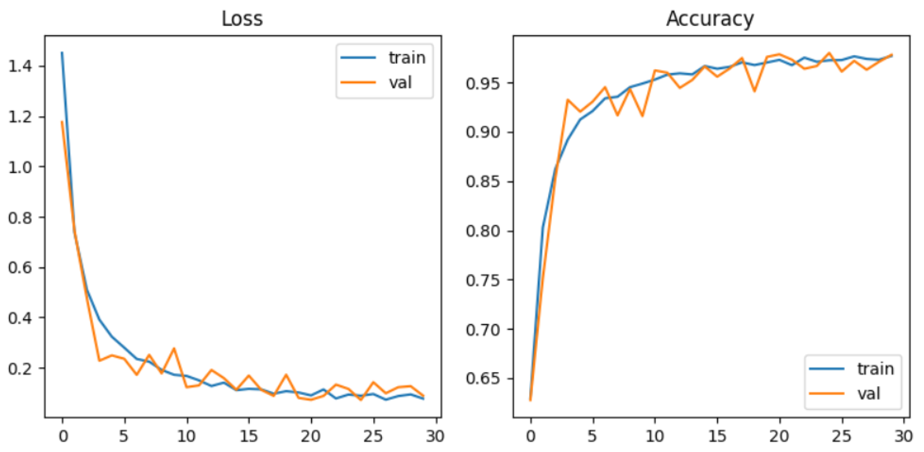
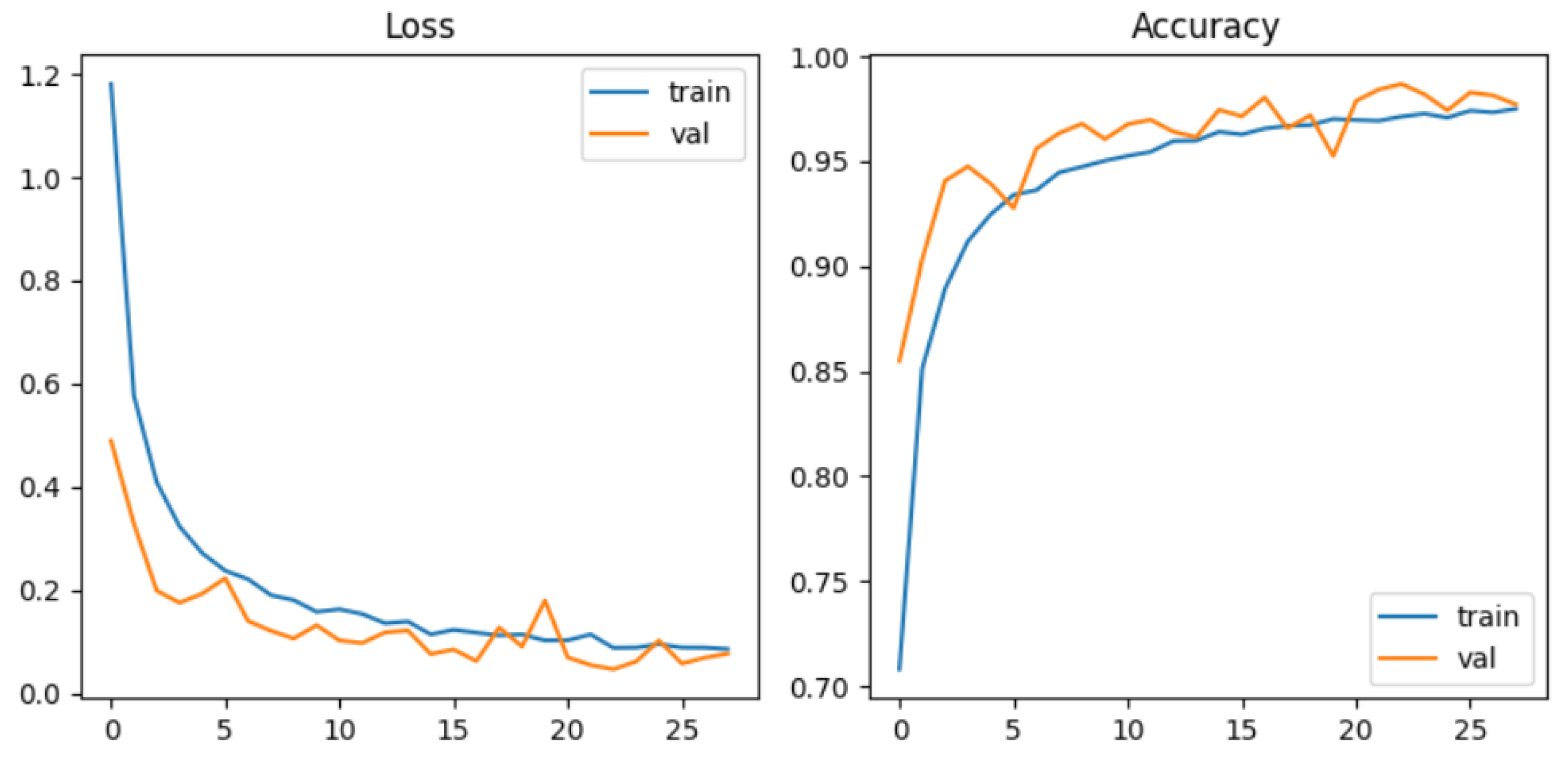
The training progress was analyzed using accuracy and loss curves, plotted from the history object that stores the training checkpoints for each epoch (Figure 5 and Figure 6).
The loss graphs show a smooth and consistent decrease, stabilizing below 0.1 around the 12th epoch, with no evidence of overfitting.
Similarly, the accuracy curves rise steadily up to 97–98%, with minimal fluctuations and a close match between training and validation trends.
These observations indicate a stable learning process and strong generalization capability, with high performance during both training and validation.
To further support these findings, a classification report was generated both for the CNN model based on the mel-spectrogram as presented in Table 1 and for the CNN model based on MFCCs shown in Table 2, confirming the model’s strong performance: just like the overall accuracy, the average F1-score was very high.
However, the model showed slight difficulty in correctly classifying instruments from underrepresented classes. For instance, the cymbals class, which had only 20 test samples, achieved good recall and F1-score values but a precision of approximately 58%, meaning that barely more than half of the model’s predictions for that class were correct.
A closer inspection of the per-class metrics highlights that some underrepresented instruments, such as cymbals, floor tom, or saxophone, achieved comparatively lower precision or recall. This outcome is expected, as these classes are represented by only a few dozen samples in the dataset, making them inherently more difficult to model reliably. In fact, the reported values can still be considered satisfactory given the extremely limited training data available. Moreover, a manual inspection of certain misclassified samples revealed that they were often of poor quality, containing background noise or ambiguous acoustic cues. Since such cases account for only a few dozen instances in the entire dataset, their impact on the overall results is limited. This highlights the persistent impact of class imbalance, which affects performance especially in categories with fewer training examples, despite the model’s overall effectiveness.
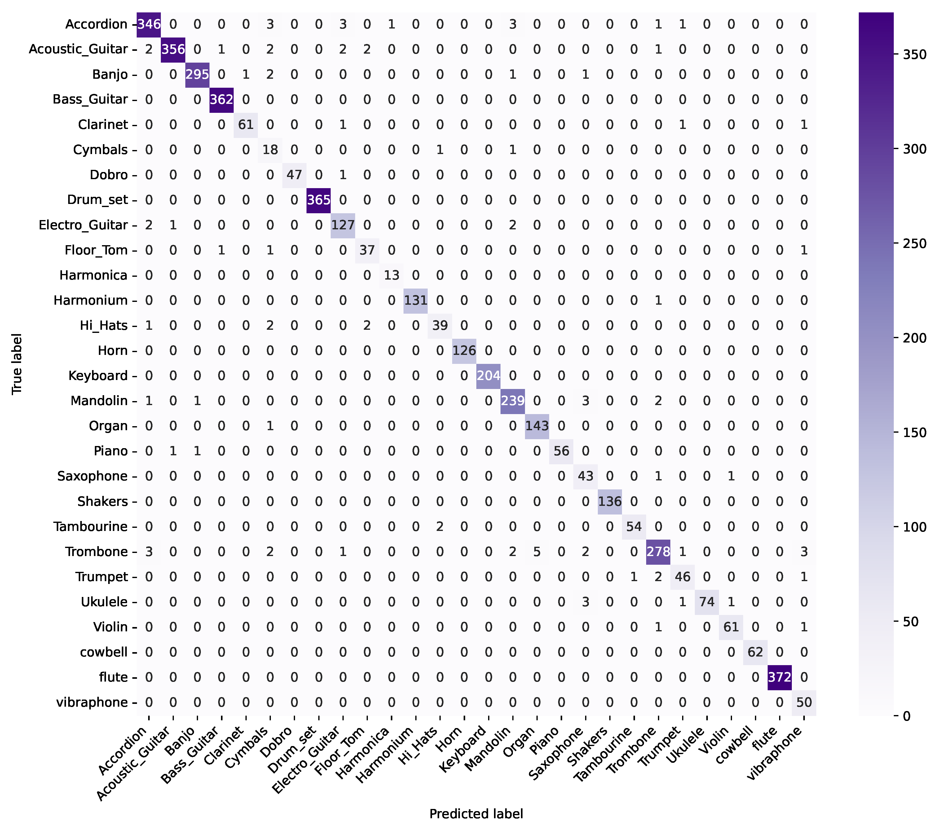
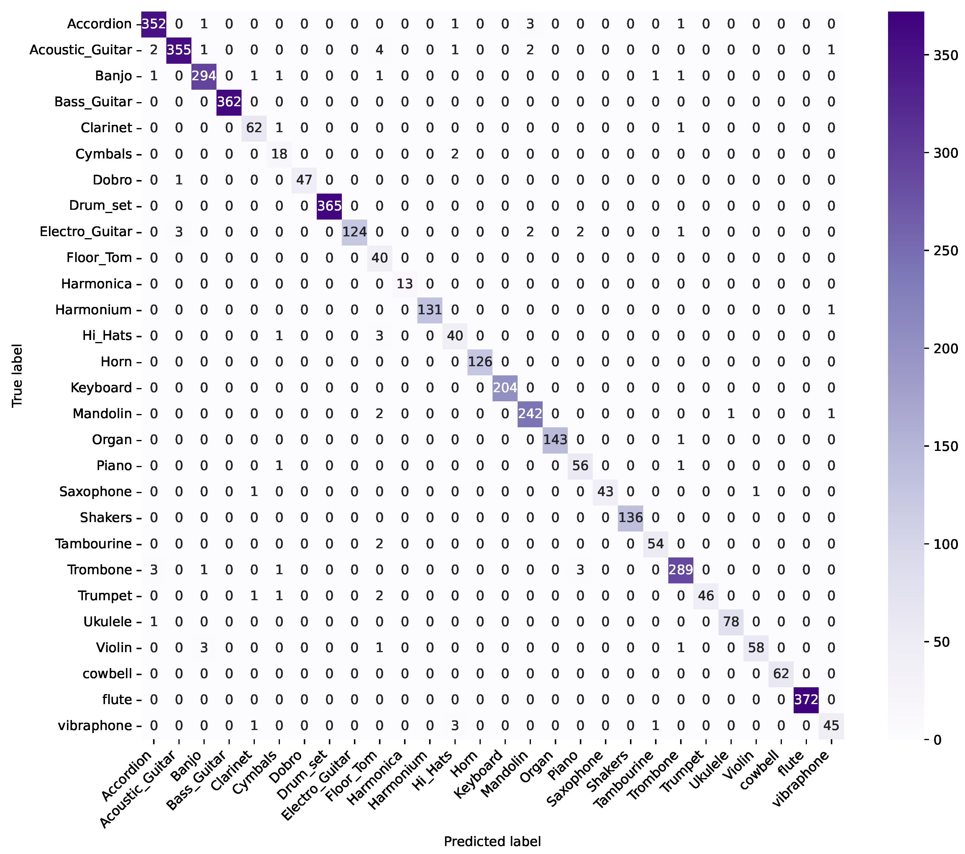
The confusion matrices shown in Figure 7 for the mel-spectogram-based CNN model and in Figure 8 for the MFCCs-based CNN model confirm the excellent classification results: most instances are correctly classified, aligning along the diagonal, which indicates robust learning and strong recognition of instrument-specific acoustic patterns.
In particular, instruments with similar timbral characteristics, such as bass guitar, accordion, harmonium, and banjo, were classified with near-perfect accuracy, suggesting the model’s ability to capture discriminative features even among acoustically related classes. Finally, greater variability was observed in the results for underrepresented classes, which remain more sensitive to the effects of data imbalance.

4.2. Explainability

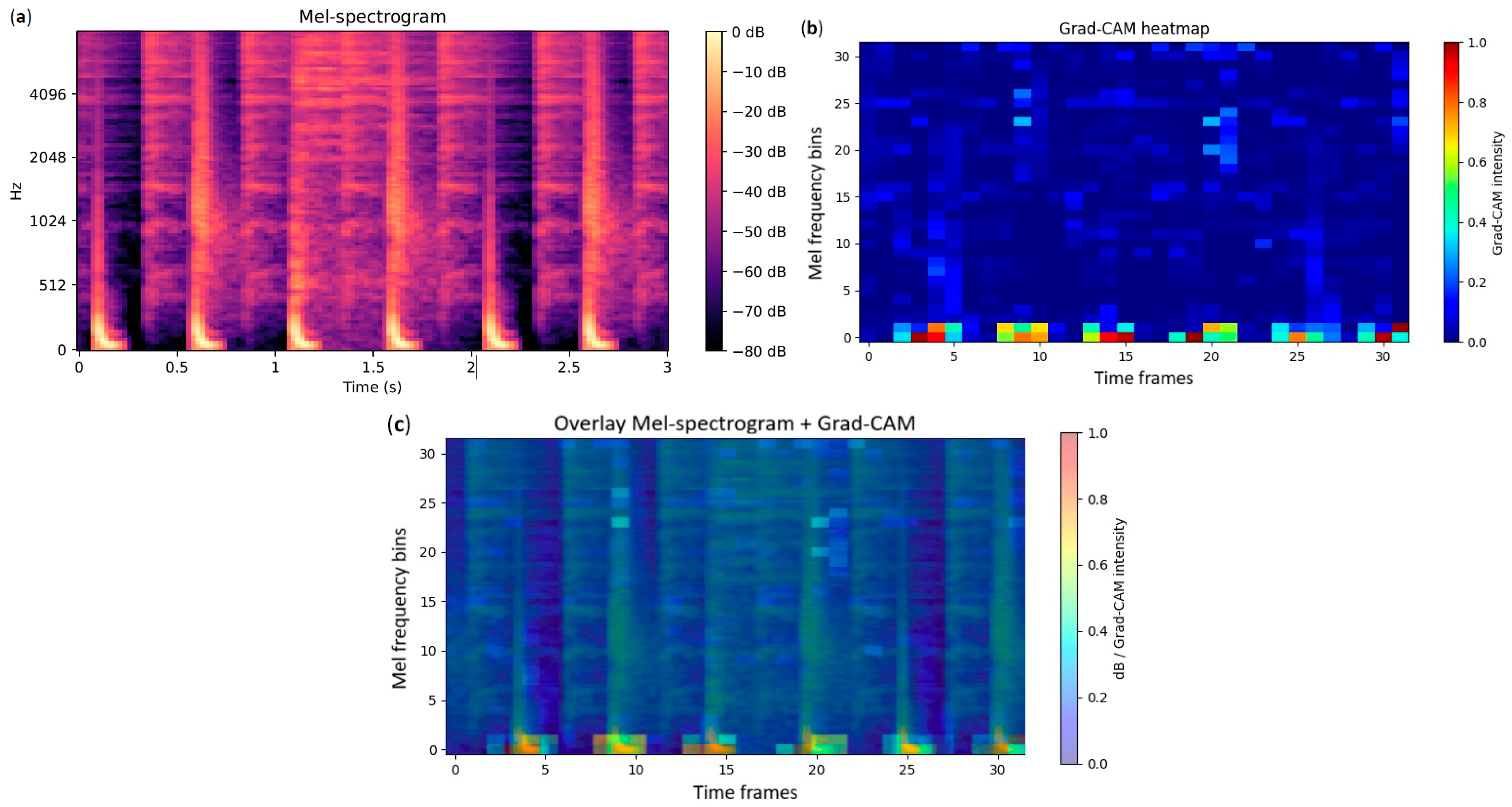
To enhance the interpretability of the audio classification model based on convolutional neural networks, the Grad-CAM (Gradient-weighted Class Activation Mapping) technique was applied to mel-spectrograms. Grad-CAM enables the visualization of the input regions that the model focuses on to make a prediction by generating a heatmap highlighting the most relevant areas. Figure 9 provides a visual comparison to facilitate interpretation: (a) the original mel-spectrogram, (b) the Grad-CAM heatmap highlighting the most informative regions, and (c) the overlay of the heatmap on the mel-spectrogram for an immediate and intuitive understanding of the model’s focus areas.
Specifically, it computes the gradient of the predicted class probability with respect to the activation maps of the model’s last convolutional layer. A spatial average of these gradients is then calculated to obtain an importance weight for each feature map, which is linearly combined with the corresponding activation maps. The resulting localized heatmap, when overlaid on the original mel-spectrogram, highlights the frequency bands and temporal segments that the network relied upon for classification.
The implementation involved configuring the model to output both the activations of the last convolutional layer and the classification prediction. Using the loss function corresponding to the predicted class, the required gradients were computed. The generated heatmap was then normalized and resized for overlay on the input mel-spectrogram, enabling clear visualization of the discriminative features detected by the model.
This approach provided a visual explanation of the model’s behavior, confirming that the highlighted regions correspond to meaningful audio patterns consistent with the performed classification.

4.3. Machine Learning Models

To compare the performance of the neural network with more traditional approaches, classification reports were generated for each model, providing precision, recall, F1-score, and support for all instrument classes across the three machine learning models: Logistic Regression (Table 3), K-Nearest Neighbors (KNN, Table 4), and Random Forest (Table 5).
Logistic Regression achieved an overall accuracy of 87.1%, with a macro-averaged F1-score of 0.82 and a weighted F1-score of 0.87. Despite reasonable performance on several classes, the model exhibited notable difficulties in discriminating between instruments with similar timbral characteristics. The confusion matrix reveals frequent misclassifications among instruments belonging to the same family, particularly for minority classes such as cymbals, saxophone, and trumpet, indicating a limited ability to model the complex, nonlinear decision boundaries required for this task.
The KNN model significantly improved classification performance, reaching an accuracy of 96.9% and a weighted F1-score close to 0.97. Previously problematic classes now show satisfactory results, although some variability remains. The confusion matrix shows a clear reduction in inter-class errors, highlighting the model’s improved robustness in identifying the distinctive acoustic features of each instrument.
The Random Forest classifier also delivered high performance, achieving an accuracy of 97% and a weighted F1-score similarly to that of KNN. Results across individual classes indicate high precision and recall, even for underrepresented instruments such as cymbals and vibraphone. While a slight drop in performance is observed for a few classes, the model demonstrates better generalization compared to Logistic Regression, particularly for minority classes, thanks to its ability to capture complex and nonlinearly separable patterns.
A detailed per-class evaluation confirms that Random Forest and KNN models achieve strong and stable results, approaching the performance of CNNs (weighted F1 ≈ 0.97), whereas Logistic Regression underperforms, especially on less frequent classes. Overall, these findings underscore the limitations of Logistic Regression in handling classification tasks involving complex audio features. In contrast, KNN and Random Forest prove to be highly effective, with KNN excelling at distinguishing instruments with overlapping characteristics and Random Forest offering greater stability, generalization, and balanced performance across all classes.

4.4. t-SNE

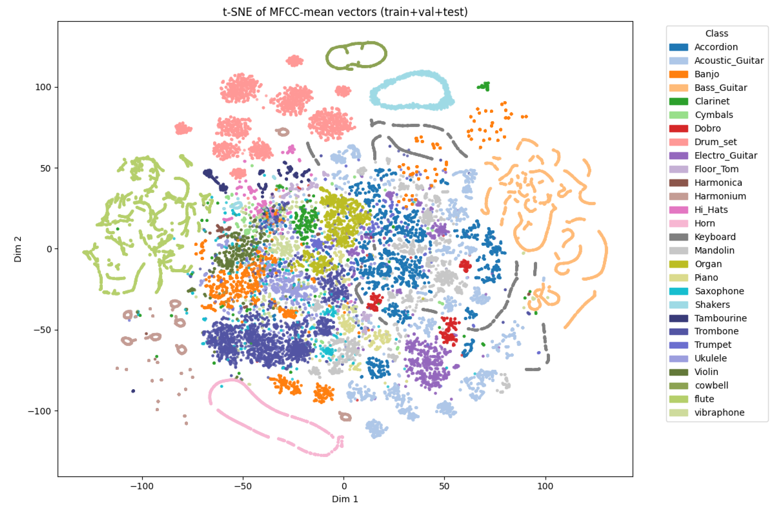
To gain a qualitative understanding of class distribution, the t-distributed Stochastic Neighbor Embedding (t-SNE) technique was applied to the entire dataset, combining training, validation, and test sets. The resulting visualization of the clustered data can be seen in Figure 10.
Each sample is represented by a mean MFCC vector of 40 coefficients, and t-SNE projects these 40-dimensional points into a two-dimensional space. This visualization provides insights into class separability and aids in interpreting the classification outcomes.
The resulting 2D map represents each audio sample as a point, colored according to its corresponding instrument class. A custom colormap of 28 distinct colors was employed to ensure clear visual distinction between all classes.
The visualization shows well-separated clusters for some classes, suggesting high separability in the original feature space, while others exhibit partial overlap, reflecting timbral similarities among certain instruments.
Despite the effectiveness of t-SNE, it is important to note that overlaps in the 2D map visualization must be interpreted with caution. First, the input representation used—mean MFCC vectors—discards temporal dynamics and compresses spectral information. Second, t-SNE is a nonlinear dimensionality reduction method, which inevitably distorts distances and local neighborhoods when projecting 40-dimensional vectors into two dimensions. Consequently, partial overlaps in the 2D plot should not be interpreted as model confusion but rather as artifacts of the embedding. Indeed, despite these overlaps, CNN models trained on richer representations, such as full MFCC sequences or mel-spectrograms, achieved very high classification accuracy, confirming that the classifiers capture discriminative patterns beyond what is visible in the low-dimensional visualization. In this study, the t-SNE map is therefore used exclusively as a qualitative tool to provide intuition about global class relationships, rather than as a definitive measure of class separability.

5. Discussion

The results obtained from the proposed instrument classification framework confirm the effectiveness of data-driven approaches in audio signal analysis. Both our CNN-based models and machine learning classifiers (Random Forest, KNN, Logistic Regression) distinguished diverse musical instruments well, despite variability in timbre, pitch, and dynamics.
Overall, the CNN demonstrated excellent classification performance, achieving near state-of-the-art results on isolated-note data. This outcome aligns with previous studies, such as Solanki & Pandey (2022) [30] and Blaszke-Kostek (2022) [31], confirming the effectiveness of convolutional architectures for instrument recognition tasks. The integration of Grad-CAM explainability further demonstrates that the network focuses on semantically meaningful spectral-temporal regions of mel-spectrograms, aligning with Chen et al. (2024) [33], who showed that MFCC and log-Mel representations tend to be the most informative, with Chroma and Tonnetz adding complementary cues. Explainability tools like Grad-CAM are therefore not only useful for visual interpretation but also essential to validate model behavior and trust its decisions, extending the results of Becker et al. (2024) [12], who emphasized the importance of interpretability in audio classification systems.
Despite this success, class imbalance remains a challenge. The marked drop in precision for rare classes such as cymbals echoes observations made in earlier studies [16,18] that classifiers often confuse acoustically similar instruments under limited training representation. Here, both deep and classical models experienced issues, though deep models were generally more robust when leveraging class weighting.
It is also noteworthy that machine learning models (KNN, Random Forest) achieved unexpectedly high performance, comparable to deep learning on this dataset. This reflects the controlled nature of the dataset (isolated, clean, short audio clips), where extracted MFCC features alone often suffice. Similar behavior has been reported in monophonic benchmarking studies with high performance using artificial neural networks (ANNs) on MFCC inputs [15,37].
Regarding feature visualization, the t-SNE embedding of averaged MFCC vectors shows partial overlaps among classes. This outcome is expected, given the lossy transformation (temporal averaging and dimensionality reduction to 2D), and should not be interpreted as a direct indication of model confusion. Instead, it provides a qualitative intuition of global class relationships. The actual reliability of the models is demonstrated by the quantitative metrics reported in this work (accuracy, F1-scores, and confusion matrices), whereas the t-SNE visualization remains only an illustrative complement.
A further element of comparison concerns computational complexity. Both CNN architectures (mel-spectrogram and MFCC inputs) were designed as lightweight models, with approximately 113k trainable parameters each. Training the mel-spectrogram CNN required about 25 min on an NVIDIA RTX Ada 500 GPU (≈50 s per epoch over 30 epochs), while the MFCC-based CNN converged faster, completing in 8 min (≈17 s per epoch). In contrast, the baseline machine learning classifiers trained on MFCC mean vectors (Logistic Regression, KNN, Random Forest) required less than one minute each, reflecting their substantially lower complexity.
Despite the differences in training time and resource requirements, CNN models offer distinctive advantages: they are inherently more robust to complex acoustic patterns, leverage richer audio representations (e.g., full time-frequency features rather than averaged descriptors), and enable explainability through Grad-CAM. Notably, inference time differences were negligible: predictions on unseen audio samples were practically instantaneous across all models. Nevertheless, for this specific dataset, traditional machine learning models proved highly competitive, achieving performance close to that of CNNs while maintaining minimal computational cost.

6. Conclusions and Future Work

The work conducted enabled the classification of musical instruments from audio files in .wav format. The two 2D convolutional neural network (2D-CNN) models, one trained on MFCCs and the other on mel-spectrograms, demonstrated highly satisfactory performance, highlighting the model’s ability to effectively recognize meaningful acoustic patterns for instrument classification.
Traditional machine learning models also performed well on this task, further confirming the relevance and quality of the extracted features. Based on the analysis of the results, it can be inferred that the dataset used is relatively simple and well-structured, allowing even simpler models to achieve good performance.
A potential enhancement of this work would be the adoption of a more complex and diverse dataset, possibly including greater timbral variability and more realistic recording conditions. An especially promising direction could involve the use of video datasets to enable multimodal classification, combining visual recognition of the instrument with its acoustic analysis.
Another possible extension would be to test the model’s efficiency in a live setting, allowing users to record audio in real time and receive immediate classification results.
Ultimately, the project could be elevated by integrating the entire system into a mobile application capable of performing real-time classification directly on a portable device, thus making the tool practical and accessible for everyday use.

Author Contributions

Conceptualization, T.S., D.N. and M.L.G.; methodology, T.S., D.N. and M.L.G.; software, T.S. and D.N.; validation, T.S. and D.N.; formal analysis, T.S. and D.N.; investigation, T.S., D.N. and M.L.G.; resources, M.L.G.; data curation, T.S. and D.N.; writing—original draft preparation, T.S. and D.N.; writing—review and editing, T.S., D.N. and M.L.G.; visualization, T.S. and D.N.; supervision, M.L.G. and A.S.; project administration, M.L.G. and A.S.; funding acquisition, M.L.G. and A.S. All authors have read and agreed to the published version of the manuscript.

Funding

This research received no external funding.

Institutional Review Board Statement

Not applicable.

Informed Consent Statement

Not applicable.

Data Availability Statement

Conflicts of Interest

The authors declare no conflicts of interest.

References

  1. Saggese, A.; Strisciuglio, N.; Vento, M.; Petkov, N. Time-frequency analysis for audio event detection in real scenarios. In Proceedings of the 2016 13th IEEE International Conference on Advanced Video and Signal Based Surveillance (AVSS), Colorado Springs, CO, USA, 23–26 August 2016; pp. 438–443. [Google Scholar] [CrossRef]
  2. Esmaili, S.; Krishnan, S.; Raahemifar, K. Content based audio classification and retrieval using joint time-frequency analysis. In Proceedings of the 2004 IEEE International Conference on Acoustics, Speech, and Signal Processing, Montreal, QC, Canada, 17–21 May 2004; Volume 5, p. V-665. [Google Scholar] [CrossRef]
  3. Zhang, W.; Xie, X.; Du, Y.; Huang, D. Speech preprocessing and enhancement based on joint time domain and time-frequency domain analysis. J. Acoust. Soc. Am. 2024, 155, 3580–3588. [Google Scholar] [CrossRef] [PubMed]
  4. Lo Giudice, M.; Mariani, F.; Caliano, G.; Salvini, A. Deep learning for the detection and classification of adhesion defects in antique plaster layers. J. Cult. Herit. 2024, 69, 78–85. [Google Scholar] [CrossRef]
  5. Lo Giudice, M.; Mariani, F.; Caliano, G.; Salvini, A. Enhancing Defect Detection on Surfaces Using Transfer Learning and Acoustic Non-Destructive Testing. Information 2025, 16, 516. [Google Scholar] [CrossRef]
  6. Abdul, Z.K.; Al-Talabani, A.K. Mel Frequency Cepstral Coefficient and Its Applications: A Review. IEEE Access 2022, 10, 122136–122158. [Google Scholar] [CrossRef]
  7. Allamy, S.; Koerich, A.L. 1D CNN architectures for music genre classification. In Proceedings of the 2021 IEEE Symposium Series on Computational Intelligence (SSCI), Orlando, FL, USA, 5–7 December 2021; pp. 1–7. [Google Scholar]
  8. Zaman, K.; Sah, M.; Direkoglu, C.; Unoki, M. A survey of audio classification using deep learning. IEEE Access 2023, 11, 106620–106649. [Google Scholar] [CrossRef]
  9. Bose, A.; Tripathy, B. Deep learning for audio signal classification. In Deep Learning—Research and Applications; De Gruyter: Berlin, Germany, 2020; pp. 105–136. [Google Scholar]
  10. Budyputra, M.A.; Reyfanza, A.; Gunawan, A.A.S.; Syahputra, M.E. Systematic Literature Review of The Use of Music Information Retrieval in Music Genre Classification. Int. J. Comput. Sci. Humanit. AI 2025, 2, 9–14. [Google Scholar] [CrossRef]
  11. Jenifer, A.E.; Abirami, K.S.; Rajeshwari, M. Enhanced Audio Signal Classification with Explainable AI: Deep Learning Approach in Time and Frequency Domain Analysis. Procedia Comput. Sci. 2025, 258, 2372–2381. [Google Scholar] [CrossRef]
  12. Becker, S.; Vielhaben, J.; Ackermann, M.; Müller, K.R.; Lapuschkin, S.; Samek, W. AudioMNIST: Exploring Explainable Artificial Intelligence for audio analysis on a simple benchmark. J. Frankl. Inst. 2024, 361, 418–428. [Google Scholar] [CrossRef]
  13. Lo Giudice, M.; Mammone, N.; Ieracitano, C.; Aguglia, U.; Mandic, D.; Morabito, F.C. Explainable deep learning classification of respiratory sound for telemedicine applications. In Proceedings of the International Conference on Applied Intelligence and Informatics, Reggio Calabria, Italy, 1–3 September 2022; Springer: Cham, Switzerland, 2022; pp. 391–403. [Google Scholar]
  14. Akman, A.; Schuller, B.W. Audio Explainable Artificial Intelligence: A Review. Intell. Comput. 2024, 3, 0074. [Google Scholar] [CrossRef]
  15. Kaminskyj, I. Automatic Source Identification of Monophonic Musical Instrument Sounds. In Proceedings of the IEEE International Conference on Neural Networks, Perth, Australia, 27 November–1 December 1995. [Google Scholar] [CrossRef]
  16. Brown, J.C. Computer identification of musical instruments using pattern recognition with cepstral coefficients as features. J. Acoust. Soc. Am. 1999, 105, 1933–1941. [Google Scholar] [CrossRef] [PubMed]
  17. Marques, J.; Moreno, P.J. A Study of Musical Instrument Classification Using Gaussian Mixture Models and Support Vector Machines. Camb. Res. Lab. Tech. Rep. Ser. CRL 1999, 4, 143. [Google Scholar]
  18. Eronen, A.; Klapuri, A. Musical Instrument Recognition Using Cepstral Coefficients and Temporal Features. In Proceedings of the 2000 IEEE International Conference on Acoustics, Speech and Signal Processing (ICASSP), Istanbul, Turkey, 5–9 June 2000. [Google Scholar] [CrossRef]
  19. Kostek, B.; Czyżewski, A. Representing Musical Instrument Sounds for Their Automatic Classification. J. Audio Eng. Soc. 2001, 49, 768–785. [Google Scholar]
  20. Livshin, A.; Rodet, X. The Importance of Cross-Database Evaluation in Sound Classification. In Proceedings of the 4th International Conference on Music Information Retrieval (ISMIR), Washington, DC, USA, 22 October 2003. [Google Scholar]
  21. Agostini, G.; Longari, M.; Pollastri, E. Musical Instrument Timbres Classification with Spectral Features. EURASIP J. Adv. Signal Process. 2003, 2003, 943279. [Google Scholar] [CrossRef]
  22. Krishna, A.G.; Sreenivas, T.V. Music Instrument Recognition: From Isolated Notes to Solo Phrases. In Proceedings of the IEEE International Conference on Acoustics, Speech, and Signal Processing (ICASSP), Montreal, QC, Canada, 17–21 May 2004; pp. 265–268. [Google Scholar] [CrossRef]
  23. Essid, S.; Richard, G.; David, B. Musical instrument recognition by pairwise classification strategies. IEEE Trans. Audio Speech Lang. Process. 2006, 14, 1401–1412. [Google Scholar] [CrossRef]
  24. Diment, A.; Rajan, P.; Heittola, T.; Virtanen, T. Modified Group Delay Feature for Musical Instrument Recognition. In Proceedings of the 10th International Symposium on Computer Music Multidisciplinary Research (CMMR), Marseille, France, 15–18 October 2013. [Google Scholar]
  25. Yu, L.; Su, L.; Yang, Y. Sparse Cepstral Codes and Power Scale for Instrument Identification. In Proceedings of the 2014 IEEE International Conference on Acoustics, Speech and Signal Processing (ICASSP), Florence, Italy, 4–9 May 2014. [Google Scholar] [CrossRef]
  26. Han, Y.; Kim, J.; Lee, K. Deep convolutional neural networks for predominant instrument recognition in polyphonic music. Ieee/Acm Trans. Audio Speech Lang. Process. 2017, 25, 208–221. [Google Scholar] [CrossRef]
  27. Lee, J.; Kim, T.; Park, J.; Nam, J. Raw Waveform-based Audio Classification Using Sample-level CNN Architectures. arXiv 2017, arXiv:1712.00866. [Google Scholar] [CrossRef]
  28. Haidar-Ahmad, L. Music and Instrument Classification using Deep Learning Techniques. 2019. Available online: https://cs230.stanford.edu/projects_fall_2019/reports/26225883.pdf (accessed on 1 October 2025).
  29. Gururani, S.; Sharma, M.; Lerch, A. An Attention Mechanism for Musical Instrument Recognition. arXiv 2019, arXiv:1907.04294. [Google Scholar] [CrossRef]
  30. Solanki, A.; Pandey, S. Music instrument recognition using deep convolutional neural networks. Int. J. Inf. Technol. 2022, 14, 1659–1668. [Google Scholar] [CrossRef]
  31. Blaszke, M.; Kostek, B. Musical Instrument Identification Using Deep Learning Approach. Sensors 2022, 22, 3033. [Google Scholar] [CrossRef]
  32. Reghunath, L.C.; Rajan, R. Transformer-based ensemble method for multiple predominant instruments recognition in polyphonic music. EURASIP J. Audio Speech Music Process. 2022, 2022, 11. [Google Scholar] [CrossRef]
  33. Chen, R.; Ghobakhlou, A.; Narayanan, A. Interpreting CNN models for musical instrument recognition using multi-spectrogram heatmap analysis: A preliminary study. Front. Artif. Intell. 2024, 7, 1499913. [Google Scholar] [CrossRef] [PubMed]
  34. McFee, B.; Raffel, C.; Liang, D.; Ellis, D.P.; McVicar, M.; Battenberg, E.; Nieto, O. librosa: Audio and music signal analysis in python. SciPy 2015, 2015, 18–24. [Google Scholar]
  35. Logan, B. Mel Frequency Cepstral Coefficients for Music Modeling. In Proceedings of the 1st International Symposium Music Information Retrieval, Plymouth, MA, USA, 23–25 October 2000. [Google Scholar]
  36. Roberts, L. Understanding the Mel Spectrogram. 2021. Available online: https://medium.com/analytics-vidhya/understanding-the-mel-spectrogram-fca2afa2ce53 (accessed on 1 October 2025).
  37. Mahanta, S.; Khilji, A.; Pakray, D.P. Deep Neural Network for Musical Instrument Recognition Using MFCCs. Comput. Y Sist. 2021, 25, 351–360. [Google Scholar] [CrossRef]
Figure 1. The bar plot visualizes the distribution of musical instrument classes within the dataset referenced in this study. Each bar indicates the number of audio samples available for a particular instrument, offering a clear overview of the dataset’s composition and the relative prevalence of each instrument class.
Information 16 00864 g001
Figure 2. Waveform of a sample audio clip from the Bass Guitar class. The x-axis represents time in seconds, while the y-axis indicates amplitude. The waveform illustrates the temporal variation in signal intensity over the standardized 3 s duration.
Information 16 00864 g002
Figure 3. Mel-spectrogram of a sample audio clip labeled “Banjo”. The x-axis represents time in seconds, the y-axis shows Mel frequency bins, and the color intensity indicates signal power in decibels (dB). Brighter regions correspond to higher energy across specific frequency bands, highlighting the spectral content of the instrument over time.
Information 16 00864 g003
Figure 4. Architecture of the 2D convolutional neural network (CNN) model used for instrument classification.
Information 16 00864 g004
Figure 5. Loss and accuracy curves for the mel-spectogram-based CNN model.
Information 16 00864 g005
Figure 6. Loss and accuracy curves for the MFCCs-based CNN model.
Information 16 00864 g006
Figure 7. Confusion matrix for the mel-spectogram-based CNN model.
Information 16 00864 g007
Figure 8. Confusion matrix for the MFCCs-based CNN model.
Information 16 00864 g008
Figure 9. Example of the steps for the explainability method Grad-CAM for the class drum set. (a) Mel-spectogram; (b) Grad-CAM heatmap; (c) overlay of Grad-CAM heatmap and mel-spectogram.
Information 16 00864 g009
Figure 10. The image displays a t-SNE plot of MFCC mean vectors. The clustering of similarly colored points suggests how well different instrument sounds are separated or grouped in the learned feature space.
Information 16 00864 g010
Table 1. Classification report for the mel-spectogram-based CNN model.
ClassPrecisionRecallF1-ScoreSupport
Accordion0.970.970.97358
Acoustic Guitar0.990.970.98366
Banjo0.990.980.99300
Bass Guitar0.991.001.00362
Clarinet0.980.950.9764
Cymbals0.580.900.7120
Dobro1.000.980.9948
Drum set1.001.001.00365
Electro Guitar0.940.960.95132
Floor Tom0.900.930.9140
Harmonica0.931.000.9613
Harmonium1.000.991.00132
Hi Hats0.930.890.9144
Horn1.001.001.00126
Keyboard1.001.001.00204
Mandolin0.960.970.97246
Organ0.970.990.98144
Piano1.000.970.9858
Saxophone0.830.960.8945
Shakers1.001.001.00136
Tambourine0.980.960.9756
Trombone0.970.940.95297
Trumpet0.920.920.9250
Ukulele1.000.940.9779
Violin0.970.970.9763
Cowbell1.001.001.0062
Flute1.001.001.00372
Vibraphone0.881.000.9350
Accuracy 0.984232
Macro avg0.950.970.964232
Weighted avg0.980.980.984232
Table 2. Classification report for the MFCCs-based CNN model.
ClassPrecisionRecallF1-ScoreSupport
Accordion0.980.980.98358
Acoustic Guitar0.990.970.98366
Banjo0.980.980.98300
Bass Guitar1.001.001.00362
Clarinet0.940.970.9564
Cymbals0.750.900.8220
Dobro1.000.980.9948
Drum set1.001.001.00365
Electro Guitar1.000.940.97132
Floor Tom0.731.000.8440
Harmonica1.001.001.0013
Harmonium1.000.991.00132
Hi Hats0.850.910.8844
Horn1.001.001.00126
Keyboard1.001.001.00204
Mandolin0.970.980.98246
Organ1.000.991.00144
Piano0.920.970.9458
Saxophone1.000.960.9845
Shakers1.001.001.00136
Tambourine0.960.960.9656
Trombone0.980.970.97297
Trumpet1.000.920.9650
Ukulele0.990.990.9979
Violin0.980.920.9563
Cowbell1.001.001.0062
Flute1.001.001.00372
Vibraphone0.940.900.9250
Accuracy 0.984232
Macro avg0.960.970.974232
Weighted avg0.980.980.984232
Table 3. Classification report for Logistic Regression.
ClassPrecisionRecallF1-ScoreSupport
Accordion0.810.650.72358
Acoustic Guitar0.910.760.83366
Banjo0.850.850.85300
Bass Guitar1.001.001.00362
Clarinet0.610.830.7064
Cymbals0.280.600.3820
Dobro0.700.960.8148
Drum set1.001.001.00365
Electro Guitar0.730.800.76132
Floor Tom0.560.880.6840
Harmonica0.871.000.9313
Harmonium1.000.991.00132
Hi Hats0.700.890.7844
Horn1.001.001.00126
Keyboard1.001.001.00204
Mandolin0.740.720.73246
Organ0.950.970.96144
Piano0.770.930.8458
Saxophone0.380.510.4445
Shakers1.001.000.99136
Tambourine0.900.930.9156
Trombone0.930.780.85297
Trumpet0.490.700.5750
Ukulele0.720.820.7779
Violin0.930.790.8563
Cowbell1.001.001.0062
Flute1.001.001.00372
Vibraphone0.490.720.5950
Accuracy 0.874232
Macro avg0.800.860.824232
Weighted avg0.890.870.874232
Table 4. Classification report for KNN.
ClassPrecisionRecallF1-ScoreSupport
Accordion0.951.000.98358
Acoustic Guitar0.981.000.99366
Banjo0.930.990.96300
Bass Guitar1.001.001.00362
Clarinet0.980.940.9664
Cymbals0.940.850.8920
Dobro0.981.000.9948
Drum set1.001.001.00365
Electro Guitar0.980.950.97132
Floor Tom0.800.970.8840
Harmonica0.871.000.9313
Harmonium1.000.991.00132
Hi Hats0.840.950.8944
Horn1.001.001.00126
Keyboard1.001.001.00204
Mandolin0.980.970.98246
Organ0.960.990.97144
Piano0.960.930.9558
Saxophone0.780.470.5845
Shakers0.991.000.99136
Tambourine0.980.950.9656
Trombone0.940.920.93297
Trumpet0.840.640.7350
Ukulele0.910.950.9379
Violin0.930.840.8863
Cowbell1.001.001.0062
Flute1.001.001.00372
Vibraphone1.000.780.8850
Accuracy 0.974232
Macro avg0.950.930.944232
Weighted avg0.970.970.974232
Table 5. Classification report for Random Forest.
ClassPrecisionRecallF1-ScoreSupport
Accordion0.951.000.97358
Acoustic Guitar0.960.990.97366
Banjo0.950.980.96300
Bass Guitar1.001.001.00362
Clarinet0.940.940.9464
Cymbals1.000.700.8220
Dobro1.000.940.9748
Drum set1.001.001.00365
Electro Guitar0.990.930.96132
Floor Tom0.911.000.9540
Harmonica1.000.920.9613
Harmonium1.000.991.00132
Hi Hats0.840.930.8844
Horn1.001.001.00126
Keyboard1.001.001.00204
Mandolin0.960.960.96246
Organ0.960.990.97144
Piano0.960.930.9558
Saxophone1.000.600.7545
Shakers1.001.001.00136
Tambourine0.960.930.9556
Trombone0.940.960.95297
Trumpet0.940.620.7550
Ukulele0.910.910.9179
Violin0.910.940.9263
Cowbell1.001.001.0062
Flute1.001.001.00372
Vibraphone0.950.840.8950
Accuracy 0.974232
Macro avg0.970.930.944232
Weighted avg0.970.970.974232
Disclaimer/Publisher’s Note: The statements, opinions and data contained in all publications are solely those of the individual author(s) and contributor(s) and not of MDPI and/or the editor(s). MDPI and/or the editor(s) disclaim responsibility for any injury to people or property resulting from any ideas, methods, instructions or products referred to in the content.