Article

Addressing Non-IID with Data Quantity Skew in Federated Learning

1
The School of Computer and Information Management, Inner Mongolia University of Finance and Economics, Huhort 010051, China
2
The School of Statistics and Mathematics, Inner Mongolia University of Finance and Economics, Huhort 010051, China
*
Author to whom correspondence should be addressed.
Information 2025, 16(10), 861; https://doi.org/10.3390/info16100861
Submission received: 21 August 2025 / Revised: 28 September 2025 / Accepted: 1 October 2025 / Published: 4 October 2025

Abstract

Non-IID is one of the key challenges in federated learning. Data heterogeneity may lead to slower convergence, reduced accuracy, and more training rounds. To address the common Non-IID data distribution problem in federated learning, we propose a comprehensive dynamic optimization approach based on existing methods. It leverages MAP estimation of the Dirichlet parameter β to dynamically adjust the regularization coefficient μ and introduces orthogonal gradient coefficients Δ i to mitigate gradient interference among different classes. The approach is compatible with existing federated learning frameworks and can be easily integrated. Achieves significant accuracy improvements in both mildly and severely Non-IID scenarios while maintaining a strong performance lower bound.

1. Introduction

Federated Learning (FL) [1,2] is an emerging distributed machine learning framework that enables knowledge sharing and user privacy protection during model training without requiring the upload of raw data. However, the statistical heterogeneity across clients, referred to as non-independent and identically distributed (Non-IID) characteristics, hinders the development of federated learning. In federated settings, datasets from a large number of clients exhibit unique attributes and usage patterns, characterized by different distributions, such as feature skew and label skew, which result in training datasets with statistical heterogeneity. Datasets with Non-IID characteristics slow down the convergence, reduce accuracy, and even result in model divergence [3]. In scenarios with high safety requirements, such as autonomous driving, model divergence caused by Non-IID data may lead to serious traffic accidents and even result in loss of life and property.
Previous works have proposed many normalization-based approaches to address the heterogeneity in federated learning. For example, FedProx [4], FedBN [5], SCAFFOLD [6], and MOON [7] have achieved relatively good performance compared to FedAvg [1]. However, these approaches struggle to adapt to datasets with varying distributions. A study [8] found that a method performing well on an IID dataset often performs worse on Non-IID data. Conversely, a method that performs better on Non-IID data often falls short on IID data, sometimes even underperforming vanilla approaches such as FedAvg, as shown in Figure 1.
Brain-inspired neural networks enhance performance under Non-IID. Mechanisms incorporating synaptic plasticity [9,10] can efficiently alleviate the catastrophic forgetting that exists in sequential learning. Moreover, brain-inspired neural networks have a vast exploration space due to synaptic plasticity and neural dynamics. In artificial neural networks (ANNs), synaptic plasticity can be interpreted as the adjustable connections between the neurons in the different layers. Synapses can be strengthened or weakened to consolidate learning and memory [11]. This process is very similar to the adjustment of model weight in the training. Research on synaptic plasticity in neural networks has made significant progress in mitigating the catastrophic forgetting [12,13,14]. Similarly, spike-timing-dependent plasticity (STDP) [15] has been applied in spiking neural networks (SNNs), achieving significant progress in reducing power consumption and also demonstrating their effectiveness in mitigating catastrophic forgetting [9,16]. Unfortunately, the integration of brain-inspired algorithms and loss function regularization remains underexplored in FL.
In this paper, we propose an algorithm that jointly incorporates a brain-inspired approach and regularization to tackle the Non-IID problem in FL. The proposed method is expected to achieve performance comparable to advanced approaches such as FedProx under IID settings, and to brain-inspired approaches such as FedNACA under Non-IID settings, as illustrated by the blue dashed line in Figure 1.
Our contributions are listed as follows:
  • We propose an approach introducing MAP-based dynamic adjustment for regularization coefficient μ in the objective function and orthogonal gradient modulation to adapt to varying degrees of Non-IID distributions. The approach is compatible with existing federated learning frameworks and can be easily integrated.
  • We propose a method to evaluate the degree of Non-IID in local datasets and mitigate model drift by adjusting the coefficient μ of the regularization term in the objective function according to the data heterogeneity.
  • We generated three datasets with different degrees of Non-IID: IID, mild Non-IID, and severe Non-IID. Extensive experimental results demonstrate that our approach achieves significant accuracy improvements in both mildly and severely Non-IID scenarios while maintaining a strong performance lower bound.

2. Related Works

2.1. Regularization-Based Approaches

Regarding Non-IID issues in FL, prior researchers have proposed various solutions, with regularization-based and brain-inspired approaches showing particularly strong performance. In machine learning, regularization-based methods were initially applied to avoid overfitting by adding a term to the objective function, thereby improving model generalization. FedProx [4] incorporated a proximal term into the loss function to alleviate statistical heterogeneity. FedDyn [17] introduced a dynamic regularization term, adding two components—a norm of the model and an inner product between the gradient and the model parameters—to enhance robustness in heterogeneous FL. Similar to these methods, SCAFFOLD [6] and MOON [7] essentially modify the loss function of neural networks to mitigate performance degradation under Non-IID settings. In HFMDS [18], the authors proposed class-relevant feature matching data synthesis by sharing partial features between the server and clients. Similarly, in the study [3], the authors also advocated sharing data between the server and clients to address Non-IID issues in FL. However, such approaches deviate from the original intent of FL. To avoid violating privacy constraints in FL, CCVR [19] shares virtual representations from higher layers of deep networks near the classifier instead of raw data to calibrate the bias of the global model caused by Non-IID. Our approach is regularization-based but differs from the above methods in that it can adapt to varying degrees of Non-IID and can be integrated with other approaches.
Adaptive/personalized FL represents another research focus for addressing the challenges posed by Non-IID in FL. Adaptive FL improves the adaptability of the global model by adjusting optimization algorithms, learning rates, aggregation strategies, and the ratio of client participation. For instance, FedNova [20] mitigates the issue of “bias accumulation” caused by inconsistent numbers of local training steps across clients, while FedOpt [21] employs adaptive optimizers at the server side to enhance the convergence speed and stability of the global model. In contrast, personalized FL aims to tackle the difficulty that a single global model cannot meet the diverse needs of clients under heterogeneous data distributions. It provides each client with a personalized model while maintaining collaborative learning. pFedMe [22] adopts a regularization-based approach such that each client learns its personalized model on top of the global model.
Non-IID problems can be interpreted as a form of catastrophic forgetting [23] in FL, and approaches designed to address catastrophic forgetting can be adapted to solve Non-IID problems in federated learning.

2.2. Biological-Inspired Approaches

Due to the intrinsic complexity of the Non-IID issues, FL has yet to establish effective and reliable solutions to address them. In contrast, intelligent biological systems do not exhibit catastrophic forgetting when learning multiple tasks, and the underlying mechanisms are continuously being explored. Biologically inspired approaches, which are capable of simulating intelligent behavior, adapting to complex and dynamic environments, and demonstrating strong robustness, as well as broad applicability within artificial intelligence, may provide valuable insights for addressing the challenges associated with Non-IID.
In recent years, researchers have proposed various heuristic algorithms inspired by biological intelligence, including mechanisms that mimic memory and synaptic consolidation, to address catastrophic forgetting [24,25], attracting significant attention. For example, ANPyC [10], an adversarial neural pruning and synaptic consolidation algorithm inspired by the memory mechanisms of mammals, provides a long-term solution to forgetting in multitask learning. Synaptic plasticity during learning is governed by principles such as Hebbian theory [26] and STDP [15]. SNNs mimic the processing and encoding of sensory information in the brain [27], and techniques developed for SNNs have been transferred to ANNs, achieving strong performance. For instance, ANNs with global neuromodulation [9] effectively mitigate forgetting issues in incremental learning. The study [28] confirmed that feedback connections in the brain deliver error signals. Similarly, the study [29] proposed synaptic intelligence, incorporating biological complexity to address forgetting of learned knowledge by introducing an importance measure for each synapse, which estimates the sensitivity of the loss function to that synapse. Synapses with lower importance to previous knowledge are adjusted to prevent interference with existing knowledge during the training of a new task.
Studies have shown that biological neuromodulation, when combined with traditional approaches, can also reduce forgetting during the acquisition of new knowledge. Inspired by the memory system of Drosophila, the study [30] proposed a solution that incorporates two additional modules compared to traditional artificial intelligence: stability protection and active forgetting. These modules enable the system to actively regulate the forgetting rate of learned knowledge while maintaining compatibility with different architectures. In the work [31], focusing on spatial behavior and drawing inspiration from neuromodulation, proposed a framework with three distinct granularities: plastic neurons based on Hebbian learning (fine-grained), layers with dropout (medium-grained), and network layers with self-regulating learning rates (coarse-grained). The authors [32] divided the neural network into multiple modules based on connection costs, where neurons within each module employ biological neural regulation mechanisms for learning, and control gates are opened to allocate a new module for acquiring new knowledge. Similarly, the authors [33] combined meta-learning with neuromodulation, dividing neural networks into multiple modules with module connections controlled by gates, as in [32]. Other works, including diffusion-based neural modulation modularization [34], differentiable neural modulation [35], neural modulation with local learning [36], and dynamic learning with neuromodulation [37], have introduced biological neuron mechanisms into neural networks to enhance performance.
Our approach differs from the aforementioned methods. Regularization typically involves adding a term to the loss function, while biological neural modulation is usually applied during weight updates; thus, the two processes operate without mutual interference. The main idea of our method is to effectively integrate regularization with biological neural modulation and validate its effectiveness in mitigating the Non-IID problem in a federated learning framework.

3. System Model

In this section, we provide a detailed description of the system model, including the federated learning architecture, The estimation of the degree of Non-IID using the MAP is based on the number of classes in the local dataset, the coefficient of the regularization term μ in the objective function, and the orthogonal tensor coefficients in the local updating stage.

3.1. Federated Learning

Let N = { 1 , 2 , , N } be a set of indices that describe N clients. In each communication round, a fraction of the clients C N is selected to train the model. The sampling ratio c = | C | | N | indicates the fraction of clients chosen per communication round due to resource constraints. Each participant i holds a local dataset D i D containing | D i | samples in the form of ( x k , y k ) , where D denotes the whole dataset, x k denotes the input vector, and y k denotes the ground truth. Let q i = { q i 1 , q i 2 , , q i r } denote the sample quantity of each class in the client i, r denote the number of classes, and | D i | = n = 1 r q i n .
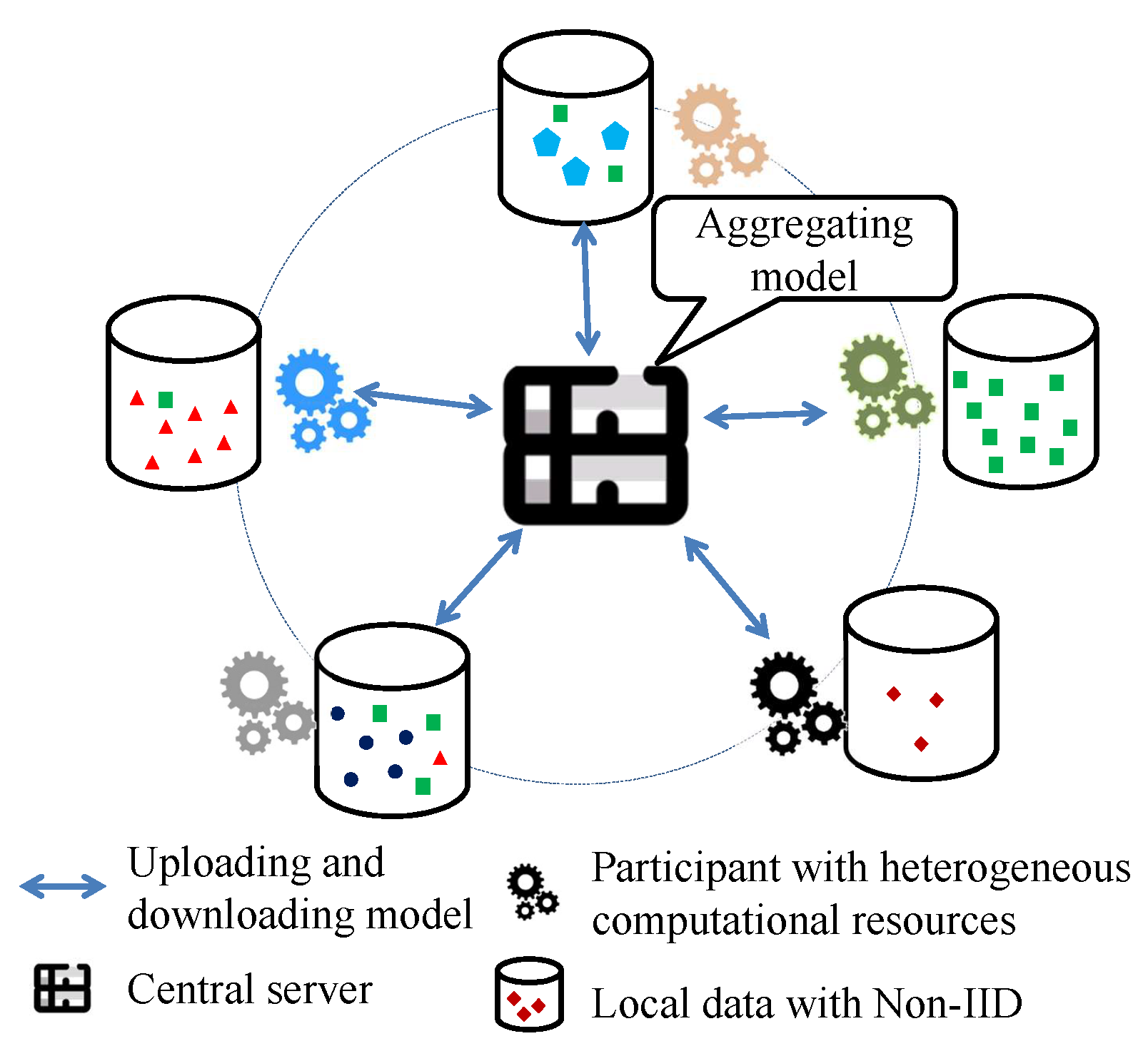
Let w i g denote the global model and w i j denote the local model on the client j in round i. Every round comprised five iterative steps: broadcasting the global model, selecting participants, the local update, uploading local model, and aggregating the model [38], as shown in Figure 2. The coefficient μ is adjusted adaptively for heterogeneous data distributions, and the normalized loss function [4] is adopted in this paper, addressing the dataset with Non-IID characteristics better. The loss function follows as
L * ( w i j ) = L ( w i j ) + μ 2 w i g w i j ,
where denotes the distance norm between two models. The coefficient of the proximal term μ 0 is related to the degree of Non-IID in the local datasets. When μ = 0 , the method reduces to FedAvg. A larger value of μ is assigned when the local datasets exhibit a higher degree of Non-IID. The coefficient μ is adaptively adjusted according to the measured degree of Non-IID. Details of the assignment strategy are provided in Section 3.2.

3.2. Evaluation for the Degree of Non-IID of Local Dataset

In Section 3.2, we first describe the characteristics of Non-IID from the perspective of class sample distribution. Then, we formulate the degree of Non-IID in the local datasets using MAP estimation with a Dirichlet prior D i r ( β ) . Finally, we discuss the relationship between the proximal term coefficient μ in the objective function and the parameter β in the Dirichlet distribution.
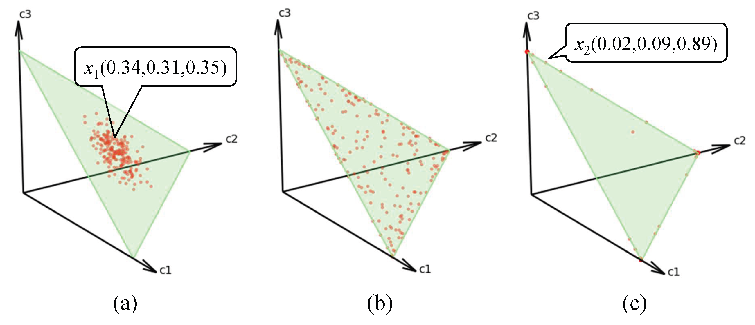
In real-world scenarios, the sample distribution across clients is typically Non-IID. In this paper, we focus on the perspective of class sample quantities, as illustrated in Figure 3. To illustrate the mechanism for quantifying the degree of Non-IID, we present an example containing a three-class dataset, as shown in Figure 4. Each dimension corresponds to a category, and each data point in the figure represents the class-wise sample distribution for a client. In Figure 4a, x 1 exhibits a nearly uniform distribution—34%, 31%, and 35% for classes c 1 , c 2 , and  c 3 , respectively, reflecting typical IID settings. Figure 4b illustrates a mild Non-IID, in which certain clients maintain balanced sample distributions, whereas others display pronounced sample count imbalances. In contrast, Figure 4c depicts a severe Non-IID, wherein client x 2 exhibits an exceptionally skewed class distribution, with 89% of its samples concentrated in class c 3 . Consequently, classes c 1 and c 2 are markedly underrepresented, leading to insufficient feature learning for these classes during local training. These scenarios can be quantitatively modeled using a Dirichlet distribution, as demonstrated in Figure 5. Figure 5 shows heatmaps of client distribution counts obtained by projecting the data from Figure 4 onto the x–y plane. In the IID setting, as Figure 5a, most clients cluster around the center area, indicating similar sample proportions across all classes. In the mild non-IID setting, as Figure 5b, the clients are more evenly dispersed, reflecting the coexistence of balanced and imbalanced distributions. In the severe non-IID setting, as Figure 5c, the majority of clients concentrate near the corners, corresponding to highly skewed distributions. These patterns are parameterized by the Dirichlet distribution with β , specifically, larger β values produce centralized distributions, as in Figure 5a, while smaller β values yield corner-concentrated distributions, as in Figure 5c. It should be noted that the parameter β of the Dirichlet distribution is r-dimensional. Assuming isotropic Dirichlet sampling, where all components of β take identical values, most studies consequently employ a single scalar parameter to characterize the degree of Non-IID.
We assume that the class quantities on each client follow a Dirichlet distribution D i r ( β ) , where β is an r-dimensional vector corresponding to the number of classes. All components of β are assumed equal, β 1 = β 2 = = β r = β , indicating an isotropic Dirichlet prior. The size of each local dataset is sampled from a uniform distribution, | D i | U ( | D | N , λ ) , where 0 λ | D | N is a variance parameter controlling the degree of Non-IID. The distribution becomes IID when λ = 0 and becomes increasingly Non-IID as λ increases.
In local training, the sample quantities are known to each client, while the parameter β of the Dirichlet distribution is unknown. The proximal term μ in the objective function significantly affects the performance of federated learning, with larger values typically assigned under severe Non-IID conditions and smaller values under near-IID conditions. We use the parameter β of the Dirichlet distribution to measure the degree of Non-IID. To this end, we employ MAP estimation to infer the posterior distribution of β given the observed class quantities as prior information.
The reason for using MAP is that the sample size provided as prior knowledge is too small during local training. Under such limited prior knowledge, MAP tends to outperform maximum likelihood estimation.
To measure the degree of Non-IID of the dataset, we treat sample quantity as a random variable. Assumption that the sample quantity q i for each participant follows D i r ( x i | β ) distribution, as shown below.
q i D i r ( x i | β ) = 1 B ( β ) j = 1 r x i j β j 1 ,
where B ( β ) denotes the Beta function, β = ( β 1 , β 2 , , β r ) denotes the parameter of the Beta function, β i > 0 and β i = β , for all i { 1 , 2 , , r } . x i j is a prior probability representing the percentage of class j in the client i, and x i j = q i j | D i | , for all j { 1 , 2 , , r } . Parameter β i of prior distribution follows Gamma distribution,
β i G a m m a ( β ; a , b ) = b a Γ ( a ) β a 1 e b β ,
where a , b are hyperparameters and β is a random variable with a > 0 ,   b > 0 ,   β > 0 . To better fit for the Non-IID setting, we choose a = 1 2 ,   b = 1 .
Posterior estimation of parameter β can be expressed as follows:
P ( β | x i ) = P ( q i | β ) P ( β ) P ( q i ) .
The computation of the denominator P ( q i ) involves a complex integral, which makes it difficult to solve directly. Considering that P ( q i ) is the constant with respect to β , and based on the relationship between posterior P ( β | q i ) and the product P ( q i | β ) P ( β ) , we adopt the MAP to estimate the parameter β . The derivation is as follows:
P ( β | x i ) P ( x i | β ) P ( β ) = 1 B ( β ) j = 1 r x j β 1 b a Γ ( a ) β a 1 e b β r
= Γ ( r β ) Γ ( β ) r j = 1 r x j β 1 1 Γ ( 0.5 ) β 0.5 e β r .
Let
L ( β ) = log Γ ( r β ) Γ ( β ) r j = 1 r x j β 1 1 Γ ( 0.5 ) β 0.5 e β r
= log Γ ( r β ) r log Γ ( β ) + ( β 1 ) j = 1 r log x j r log Γ ( 0.5 ) + 1 2 log β + β .
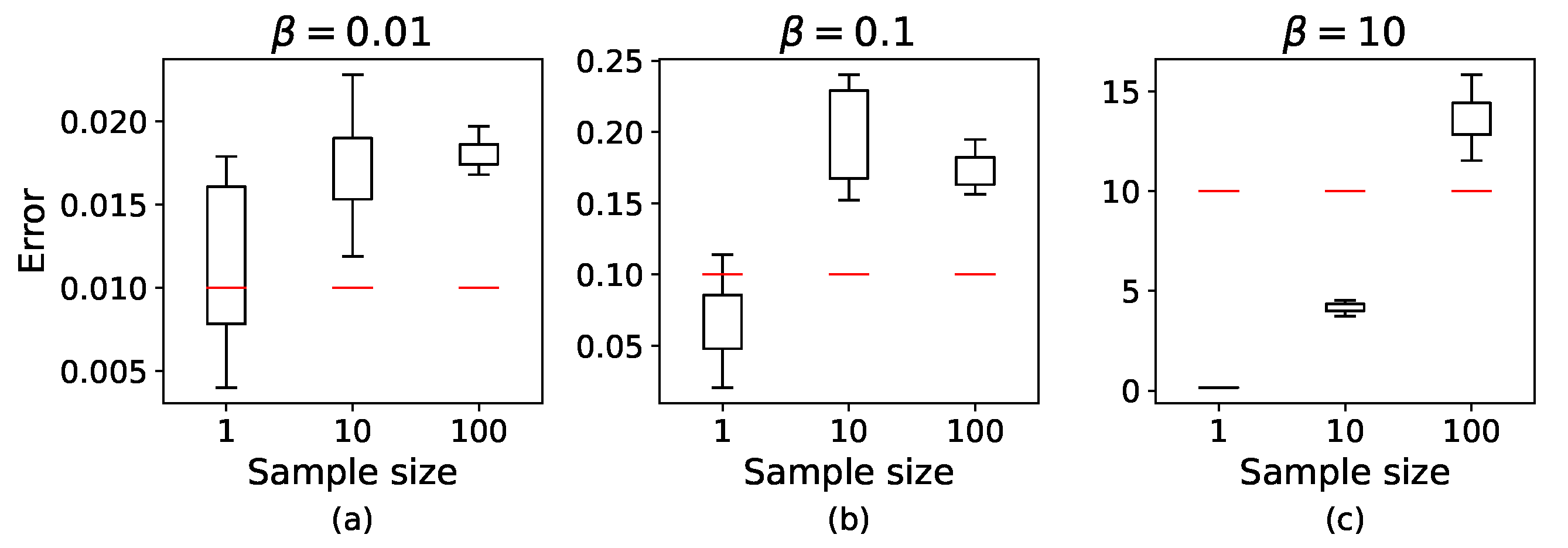
Since the MAP estimate lacks a closed-form solution, the Newton–Raphson method is used to obtain a numerical estimate of β . To evaluate the effectiveness of this numerical solution, we run the program 10 times under each setting. The results are illustrated with error bars in Figure 6. The numerical estimates perform well under Non-IID settings, while noticeable deviations from the true value are observed under IID conditions. This is because the final MAP estimate is influenced by the hyperparameters a , b in the Gamma prior distribution.
In MAP estimation, the bias and variance are influenced by the prior knowledge and the sample size, and are generally smaller than those of the MLE. In this work, since the dataset exhibits the more severe Non-IID characteristics, the parameters of the prior distribution are set to favor these severe Non-IID scenarios. As a result, when the dataset exhibits IID characteristics, the bias and variance of the MAP estimator tend to increase. This issue can be addressed via a μ β mapping. Specifically, when the MAP estimate of β exceeds a certain threshold, the dataset is considered IID, and an IID-specific approach is employed for training.

3.3. Relationship Between μ and β

The degree of Non-IID in a dataset significantly influences both the performance and convergence speed of the model. Introducing a proximal term into the objective function can improve performance when training on heterogeneous data. However, this regularization term may also impair the model’s generalization ability. Therefore, datasets with different levels of Non-IID are not suitable for using the same value of μ . For instance, the proximal term μ should be set to 0 for IID datasets. In contrast, for datasets with severe Non-IID, a larger μ is desirable to enhance generalization.
In this paper, we adopt the β parameter introduced in the previous section, which not only quantifies the degree of Non-IID in the dataset but also serves as a basis for estimating a suitable value of μ . This enables the objective function to adapt automatically to varying levels of data heterogeneity. A simple piecewise nonlinear mapping between μ and β is designed, as shown below.
μ = A 0 , β β 0 A 0 β 0 10 β , β 0 < β < β 1 0 , β β 1 ,
where β is the variable, and  A 0 > 0 is a real-valued constant to control the magnitude of the proximal term. β 0 and β 1 are fixed thresholds. The mappings are illustrated in Figure 7. A smaller β indicates a more severe Non-IID distribution, which corresponds to a larger value of μ , and vice versa. When the estimated β exceeds β 1 , the dataset is considered to be IID, and  μ is set to zero. In this case, the proximal term vanishes, and the objective reduces to that of standard federated learning. When β < β 0 , μ is assigned a constant value A 0 . If  A 0 is set too large or tends toward infinity, the objective function may degenerate into a mean squared error (MSE), overwhelming the original loss function. Therefore, it is advisable to avoid setting A 0 excessively large. Based on experimental comparisons, the setting β 0 = 0.01 , β 1 = 1 and 1 A 0 4 yields relatively better performance [4].
The output metrics are largely insensitive to variations in the μ β mapping and the latent variables, such as the parameters a and b of the Gamma function in the prior distribution. The effect of parameter changes on the outputs is predictable and exhibits a clear pattern. Moreover, the outputs are primarily governed by the characteristics of the dataset distribution, indicating a high degree of robustness.

3.4. Controlling Gradient Coefficient Δ i

Given that regularization-based objective functions offer limited improvement under Non-IID conditions and may, to some extent, hinder convergence. To this end, we introduce a mutually orthogonal coefficient, Δ ( j ) , j = 1 , 2 , , r , to control the gradient and isolate the interference among the knowledge. The coefficient Δ ( j ) is a tensor with the same shape as the model, and each class is assigned a coefficient. These coefficients are mutually orthogonal under the Frobenius inner product, ensuring minimal interference among classes and satisfying orthogonality under the Frobenius inner product, and as follows:
T r ( Δ ( i ) T , Δ ( j ) ) = 0 , i j T r ( Δ ( i ) T , Δ ( j ) ) = 1 , i = j ,
where T r ( · , · ) represents the sum of the main diagonal elements after the multiplication of two tensors with the same dimensions.
The intuitive rationale behind introducing inter-class orthogonal coefficients is based on the assumption that feature representation spaces corresponding to different classes are mutually exclusive. This assumption is well-justified in practice, as objects from distinct categories typically exhibit unique, non-overlapping characteristics.
Next, client k generates its coefficients based on the local data distribution using the following formula:
Δ k = i = 1 r x k i Δ ( i ) ,
where x k i = q k i j q k j is a scalar that performs element-wise multiplication with the tensor Δ ( i ) . For details on the generation of Δ ( i ) , please see Appendix A.
In the round ( i + 1 ) t h , the model parameters on client k are updated according to the following formula:
w i + 1 k = w i k l r ( Δ k L * w ) ,
where l r denotes the learning rate, and ⊙ denotes element-wise multiplication. It should be noted that Δ ( i ) denotes a class-specific constant tensor, whereas Δ k represents a coefficient computed by client k according to the characteristics of its local data distribution.
This idea is inspired by the concept of global synaptic plasticity in computational neuroscience [9]. In the brain, neuromodulatory substances such as dopamine and serotonin regulate synaptic plasticity. These neuromodulators play a key role in modulating the plasticity mechanisms themselves—a phenomenon often referred to as the "plasticity of plasticity"—which enables the brain to accelerate learning and enhance memory consolidation, as illustrated in Figure 8.
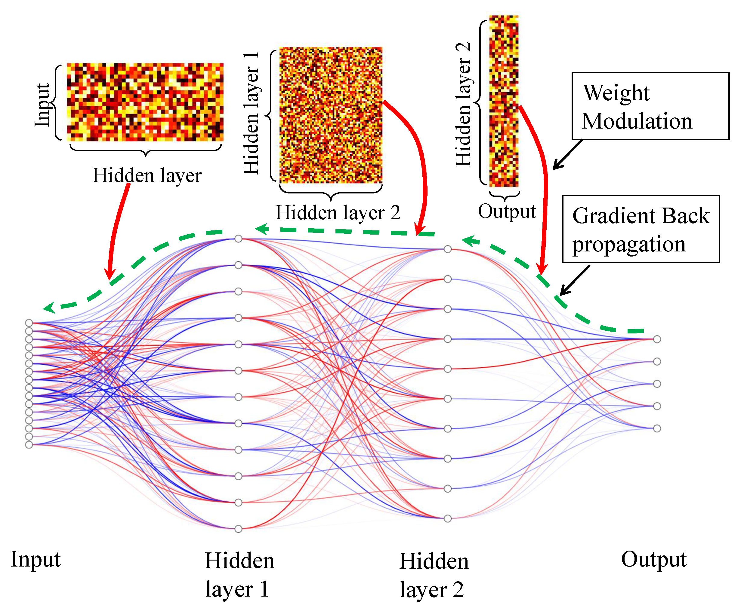
This modulation process can be mathematically formulated as shown in Equation (12), where Δ k represents the global neuromodulator, and  L * w corresponds to synaptic plasticity governed by Hebbian learning rules [26], as depicted in Figure 9.
To clarify the construction procedure of our approach to improve reproducibility and implementation guidance, the pseudocode for the implementation is provided in Algorithm 1.
Algorithm 1 The pseudocode of the proposal
1:
Generate Δ ( i ) For class i according to Appendix A at the server side
2:
Broadcast Δ ( i ) to all clients
3:
Client k calculates Δ k according to Δ k = i = 1 r x k i Δ ( i )
4:
repeat
5:
   Broadcasting global model to all clients
6:
   Local update according to w i + 1 k = w i k l r ( Δ k L * w ) at client side
7:
   Aggregate local model
8:
until Global_epoch > Predefined_value

3.5. Convergence Analysis

The convergence analysis of the proposed approach in this paper is divided into two parts: one concerns the convergence of the objective function with the regularization term, and the other concerns the convergence of the weight updates with orthogonal coefficients. The convergence of the objective function with the regularization term has been thoroughly examined in work [4]. The MAP-based estimation of the regularization coefficient employed in our approach does not affect the convergence property. Therefore, we focus on analyzing the convergence of the weight updates with orthogonal coefficients.
Lemma 1.
Let Δ i F = 1 , i = 1 , 2 , , r , and  < Δ i , Δ j > F = 0 , i j , where · F is the Frobenius norm, < · , · > F is Frobenius inner product, Δ = i = 1 r w i Δ i , where 0 w i 1 is a scalar and i = 1 r w i = 1 , then Δ F 1 .
Proof of Lemma 1.
 Since < Δ i , Δ j > F = 0 for i j and Δ i F = 1 , we have
Δ F 2 = < i = 1 r w i Δ i , j = 1 r w j Δ j > F = i = 1 r j = 1 r w i w j < Δ i , Δ j > F = i = 1 r w i 2
because all cross terms vanish.
0 w i 1 , then
Δ F = i = 1 r w i 2 i = 1 r w i = 1 .
Taking square roots yields Δ F = 1 .    □
We provide a convergence analysis under the assumption that the loss function is convex. The extension to the non-convex setting has been extensively studied in the prior works [4,6,39,40], and the corresponding conclusions can be straightforwardly generalized.
Assumption that the objective function L * ( w i ) satisfied following conditions:
  • L-smoothness: L * ( w i ) L * ( w j )   L 2 w i w j 2 .
  • Strong convex: L * ( w i ) L * ( w j ) + ( w i w j ) T L * ( w j ) + μ 2 w i w j .
  • Bounded gradient: E L * ( w i ) L * ( w * ) 2   σ 2
Theorem 1.
The proposed approach exhibits the same convergence properties as the FedProx [4], specifically, w * w i + 1 o u r s     w * w i + 1 f e d p r o x .
Proof of Theorem 1.
w * w i + 1 o u r s   =   w * w i o u r s l r * ( Δ L * ( w i ) )
According to Lemma 1,
w * w i o u r s l r * ( Δ L * ( w i ) )   w * w i o u r s + l r * L * ( w i ) = w * w i + 1 f e d p r o x
where · represents the distance norm.
The convergence of w * w i + 1 f e d p r o x has been proved in the work [4]. Thus, our approach also achieves convergence.    □

4. Experiments

In our experiments, we compare the proposed method with several classical federated learning baselines, including FedAvg [1], FedProx with μ = 0.2 [4], SCAFFOLD [6], MOON [7], and FedNACA [9]. To evaluate and compare the convergence speed of these approaches, we employ a two-layer neural network with 1,000 neurons in the hidden layer.
The experiments are conducted on two widely used benchmark datasets: MNIST [41] and CIFAR10 [42]. To simulate varying degrees of data heterogeneity, we synthesize three different non-IID datasets using the Dirichlet distribution [43] with concentration parameters β = 1000 ,   β = 0.5 , and  β = 0.01 , which correspond to IID, mild Non-IID, and severe Non-IID scenarios, respectively. The IID dataset contains all classes of samples, and the quantity of the class is equal to each other. Mild and severe Non-IID datasets are generated by Dirichlet distribution with the setting β = 0.5 and β = 0.01 , respectively. In Non-IID datasets, both the number of classes and the number of samples are imbalanced across clients. During the experiments, the client can only access the number of samples for each class in its local dataset, and the value of the parameter β is unknown, which is estimated by MAP. The dataset is partitioned into 10 non-overlapping subsets, and each subset is assigned to a distinct client.

4.1. Metrics

To evaluate the convergence speed of different methods, we employ two metrics: (1) the number of communication rounds required to reach a predefined target accuracy and (2) the top-1 accuracy. In each communication round, a fraction of clients, referred to as the sampling ratio 0 < C 1 , is randomly selected to participate in model training; while both metrics capture aspects of convergence, the number of rounds to reach the target accuracy provides a more intuitive and direct measure of convergence speed across different algorithms compared to tracking accuracy curves. All experiments are conducted over 100 communication rounds.

4.2. Results on Non-IID Degree and Client Sampling Ratio C

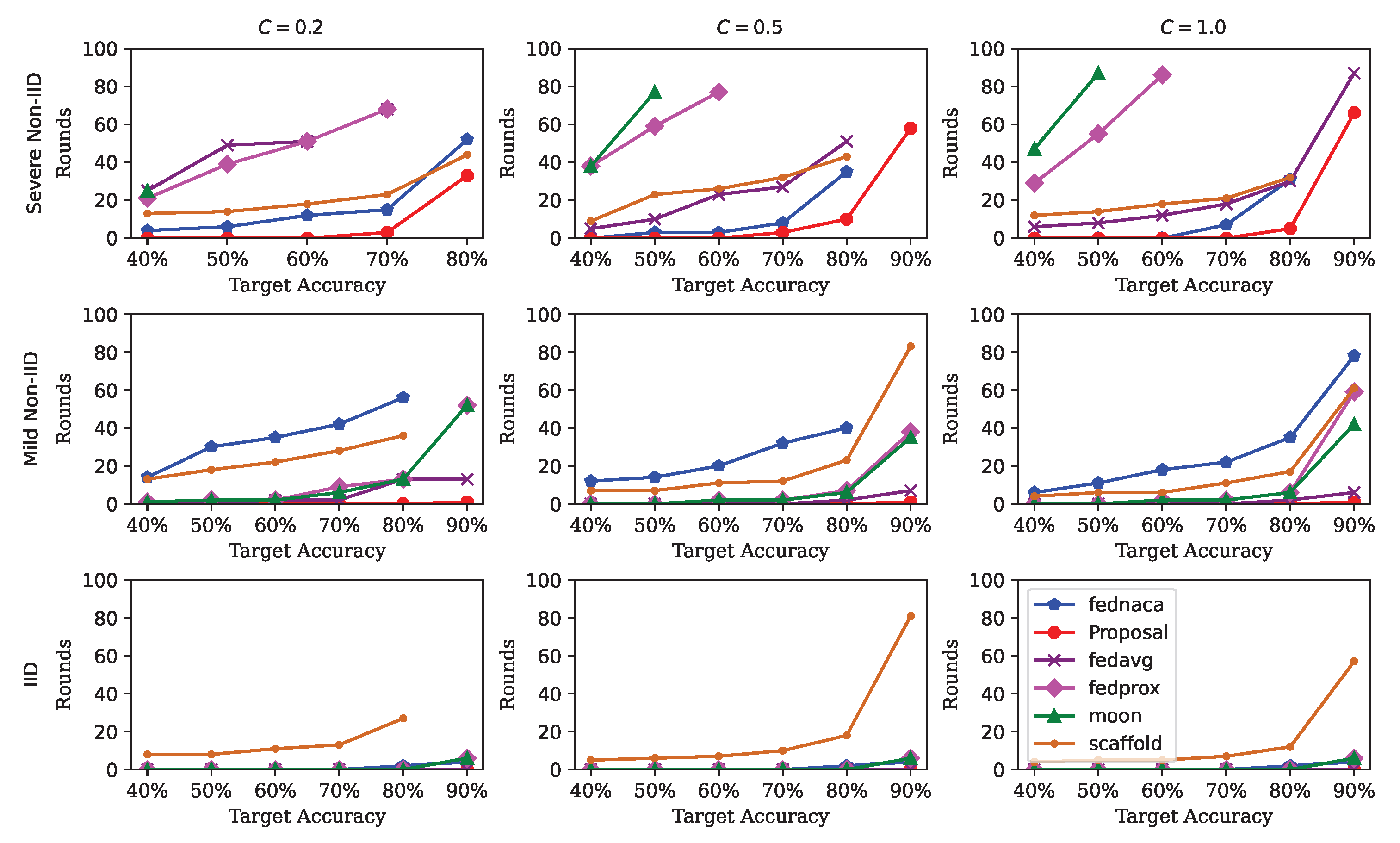
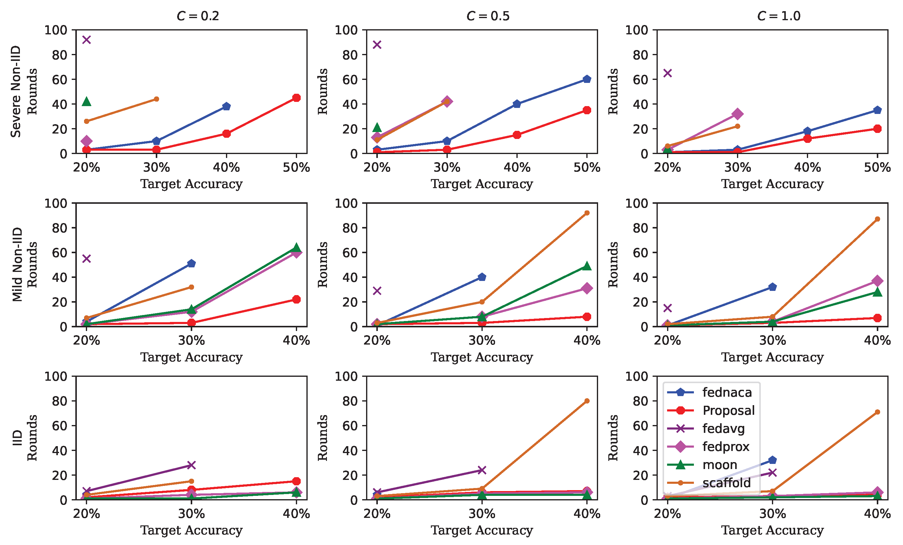
We conduct experiments with varying degrees of Non-IID and client sampling ratios on the MNIST and CIFAR-10 datasets. The results are presented in Figure 10 and Figure 11. In both figures, the x-axis denotes the target accuracy, while the y-axis indicates the number of communication rounds required to achieve target accuracy. A steeper slope corresponds to a greater number of rounds needed, reflecting slower convergence, and vice versa.
Figure 10 and Figure 11 illustrate the effects of two parameters: the degree of Non-IID and the client sampling ratio. The degree of Non-IID is categorized into three levels: IID, mild Non-IID, and severe Non-IID. The client sampling ratio C takes values in 0.2 , 0.5 , 1.0 .
From the figures, several observations can be made. First, under a fixed Non-IID setting (i.e., subplots within the same row, from left to right), all algorithms exhibit faster convergence as C increases. This implies that increasing the number of participating clients leads to improved model generalization. Second, as the data distribution shifts from IID to severe Non-IID (i.e., subplots within the same column, from bottom to top), the performance of all algorithms degrades significantly, indicating that data heterogeneity substantially impacts convergence behavior. Third, regarding convergence speed, our proposed method consistently outperforms other baselines in both mild and severe Non-IID scenarios, while maintaining comparable performance under IID settings.
These improvements primarily arise from two key aspects. First, unlike the fixed proximal term in FedProx, we estimate the hyperparameter μ via MAP estimation, enabling it to adapt dynamically to different degrees of Non-IID. Consequently, our method surpasses both FedProx and FedAvg in performance. Second, during the parameter update phase, we introduce an orthogonalized coefficient tensor that is element-wise multiplied with the gradient. This operation effectively isolates the representations of different classes or knowledge components, thereby mitigating mutual interference—a feature absent in FedNACA.
Some approaches, such as FedAvg, exhibit poor performance under conditions of low client sampling ratios and severe Non-IID data distributions, as illustrated in the first subplot of the first row in Figure 10. After 100 rounds of training, FedAvg achieves an accuracy of only 20%. This suboptimal performance can be partly attributed to the relatively small model size. Nevertheless, increasing the model capacity leads to some improvement in accuracy. Additionally, the limited number of training rounds suggests that, under the current experimental settings, FedAvg’s convergence speed is comparatively slow.

4.3. Results on Top-1 Accuracy

The number of communication rounds required to reach the target accuracy serves as a measure of the convergence speed of each approach, whereas the top-1 accuracy reflects the model’s reliability. The top-1 accuracies of all baseline methods after 100 rounds are summarized in Table 1. As shown in Table 1, our proposed method achieves higher top-1 accuracy than most other approaches under both mild and severe Non-IID settings. Under the IID setting, although the accuracy difference between our method and the highest top-1 accuracy reaches up to 6.55%, our approach is still not the worst-performing approaches.
Two main factors contribute to these observations. First, during the estimation of β via MAP, the parameters of the prior Gamma distribution ( a = 1 2 ,   b = 1 ) are better suited for Non-IID scenarios. When the data distribution is IID, this prior introduces some bias in the estimation of β . Second, the mapping function between β and μ does not fully capture the true variation, leading to certain estimation errors, as illustrated in Figure 7 and Equation (9).

5. Conclusions

In this paper, we propose a novel approach to address the challenges posed by Non-IID data distributions in federated learning. The proposed approach comprises two key components. First, a new proximal term coefficient is incorporated into the objective function, where the coefficient is derived via Maximum A Posteriori (MAP) estimation based on the local sample statistics to quantitatively reflect the degree of data heterogeneity. Second, to mitigate model drift and reduce inter-class interference during updates, an orthogonal tensor coefficient is assigned to each class. This coefficient modulates the gradient through element-wise multiplication, thereby preserving class-specific knowledge. Extensive experiments conducted on benchmark datasets demonstrate the effectiveness and robustness of the proposed method in comparison with classical baselines under varying degrees of data heterogeneity.

Author Contributions

N.C. was responsible for coding, running simulations, and processing the results. L.C. was responsible for modeling, deriving proofs, and writing the manuscript. All authors contributed equally. All authors have read and agreed to the published version of the manuscript.

Funding

This work was supported by the Program for High-Quality Research Achievement of Inner Mongolia University of Finance and Economics (No. GZCG24208, No. NCXKY25050), and the Natural Science Foundation of Inner Mongolia (No. 2024LHMS01010).

Institutional Review Board Statement

Not applicable.

Informed Consent Statement

Not applicable.

Data Availability Statement

The original data presented in the study are openly available on GitHub at https://github.com/nrs018/Non-IID_FL (version 1.0, accessed on 10 August 2025).

Conflicts of Interest

The authors declare no conflicts of interest.

Appendix A. Generation of Δ (i)

Figure A1. The red line represents that there is a connected path from the input to the output in Δ ( i ) . The size of input and output are n and k, respectively.
Information 16 00861 g0a1
In this paper, Δ ( i ) is generated for each class i, and it is required to satisfy the following conditions:
i
< Δ ( i ) , Δ ( j ) > F = 0 , i j , where < · , · > F represents the Frobenius inner product, is the Euclidean norm of a matrix. Requiring the Frobenius inner product to be zero implies that Δ ( i ) corresponding to different classes do not overlap, which can be interpreted as the features of different classes being distinguishable.
ii
0 δ j , k ( i ) 1 , for any element δ j , k of Δ ( i ) . This condition indicates that the magnitude of a model weight update is less than or equal to the corresponding gradient. When δ j , k ( i ) = 0 , the corresponding weight will be frozen, implying that this weight does not contribute to the given class. When δ j , k ( i ) = 1 , the corresponding weight will be updated according to the gradient without any reduction.
iii
In Δ ( i ) , at least, a path connects from input to output, illustrated by the simplified two-layer fully connected network in Figure A1. Similar to the model, Δ ( i ) also can be decomposed into multiple layers of parameters, represented as multiple tensors, δ n × m ( 1 ) , δ m × k ( 2 ) represent the parameters of the first layer, second layer,..., respectively. The path from the input to the output is expressed as δ n × m ( 1 ) · δ m , k ( 2 ) , in which there exists at least one element of the multiplication of two tensors a j , k > 0 , as shown the red line in Figure A1. In our experiments, we set the threshold for the element to ensure the parameters of the model are activated.
The reason for introducing the condition (iii) is to prevent all parameters in a certain layer of Δ ( i ) from becoming zero. In such a case, the neural network would no longer be able to continuous learning.
Algorithm A1 the implementation of Δ ( i )
1:
repeat
2:
   Randomly generate r tensors with the same dimensions as the model
3:
   Flatten all tensors into 1-dimensional vectors
4:
   Apply the Gram–Schmidt orthogonalization to orthogonalize the r tensors
5:
   for Each tensor do
6:
     if Check if a tensor has transitivity using Algorithm A2 then
7:
        GOTO step 2
8:
     end if
9:
   end for
10:
until Obtain r tensors that are orthogonal and satisfy the transitivity property
11:
Normalize each tensor to 0 < δ j , k ( i ) 1
12:
Reshape the tensor to match the dimensions of the model
Algorithm A2 Check the transitivity of the tensor
Require:
Input a 1-dimensional tensor, class i
Ensure:
Output a boolean value ▹ TRUE: no transitivity, FALSE: have transitivity
1:
Initialize L_weight = 0
2:
Reshape the tensor as same the dimensions of the model
3:
for Each layer in model do
4:
   L_weight = L_weight * weight of layer i
5:
end for
6:
for element in row i of L_weight do
7:
   if element > threshold then
8:
     return FALSE                     ▹ have transitivity
9:
   end if
10:
end for
11:
return TRUE                       ▹ no transitivity
The idea of introducing Δ ( i ) originates from the work [44,45,46], but with some differences. First, Δ ( i ) is only related to the classification features and remains unchanged throughout the entire training process. Second, in federated learning, Δ ( i ) is obtained from the server to ensure that all clients have the same delta, and it is not uploaded to the server during each communication round.
To clarify the implementation of Δ ( i ) , a detailed description is presented in Algorithm A1. The main idea of this algorithm is to first construct r mutually orthogonal tensors using the Gram–Schmidt orthogonalization, and then verify for each tensor whether a path exists from the input layer to the classification layer. This can be achieved by checking whether a transitive relation exists between the input nodes and the classification nodes.
Next, we analyze the complexity of the algorithm. The Gram–Schmidt orthogonalization process for r tensors has a complexity of O ( r | w | ) , where | w represents the number of parameters in the model. Subsequently, r represents the number of classes, and the Warshall algorithm is applied to each tensor to verify whether a transitive relation exists between the input and output nodes, with a complexity of O ( | w | 3 ) . The brute-force search further introduces a complexity of O ( | C | ) , where | C | represents the size of the search space. Therefore, the overall complexity of the algorithm can be expressed as O ( r | w | 4 | C | ) .

References

  1. McMahan, B.; Moore, E.; Ramage, D.; Hampson, S.; Arcas, B.A.y. Communication-Efficient Learning of Deep Networks from Decentralized Data. In Proceedings of the 20th International Conference on Artificial Intelligence and Statistics, Fort Lauderdale, FL, USA, 20–22 April 2017; pp. 1273–1282. [Google Scholar]
  2. Yang, Q.; Liu, Y.; Chen, T.; Tong, Y. Federated machine learning: Concept and applications. Acm Trans. Intell. Syst. Technol. (TIST) 2019, 10, 1–19. [Google Scholar] [CrossRef]
  3. Zhao, Y.; Li, M.; Lai, L.; Suda, N.; Civin, D.; Chandra, V. Federated Learning with Non-IID Data. arXiv 2018. [Google Scholar] [CrossRef]
  4. Li, T.; Sahu, A.K.; Zaheer, M.; Sanjabi, M.; Talwalkar, A.; Smith, V. Federated Optimization in Heterogeneous Networks. In Proceedings of the Machine Learning and Systems (MLSys 2020), Austin, TX, USA, 2–4 March 2020; Volume 2, pp. 429–450. [Google Scholar]
  5. Li, X.; Jiang, M.; Zhang, X.; Kamp, M.; Dou, Q. FedBN: Federated Learning on Non-IID Features via Local Batch Normalization. arXiv 2021. [Google Scholar] [CrossRef]
  6. Karimireddy, S.P.; Kale, S.; Mohri, M.; Reddi, S.; Stich, S.; Suresh, A.T. SCAFFOLD: Stochastic Controlled Averaging for Federated Learning. In Proceedings of the 37th International Conference on Machine Learning, PMLR, Virtual, 13–18 July 2020; pp. 5132–5143. [Google Scholar]
  7. Li, Q.; He, B.; Song, D. Model-Contrastive Federated Learning. In Proceedings of the IEEE/CVF Conference on Computer Vision and Pattern Recognition, Nashville, TN, USA, 20–25 June 2021; pp. 10713–10722. [Google Scholar]
  8. Dohare, S.; Hernandez-Garcia, J.F.; Lan, Q.; Rahman, P.; Mahmood, A.R.; Sutton, R.S. Loss of plasticity in deep continual learning. Nature 2024, 632, 768–774. [Google Scholar] [CrossRef]
  9. Zhang, T.; Cheng, X.; Jia, S.; Li, C.T.; Poo, M.-M.; Xu, B. A brain-inspired algorithm that mitigates catastrophic forgetting of artificial and spiking neural networks with low computational cost. Sci. Adv. 2023, 9. Available online: https://www.science.org/doi/10.1126/sciadv.adi2947 (accessed on 10 August 2025). [CrossRef]
  10. Peng, J.; Tang, B.; Jiang, H.; Li, Z.; Lei, Y.; Lin, T.; Li, H. Overcoming long-term catastrophic forgetting through adversarial neural pruning and synaptic consolidation. IEEE Trans. Neural Netw. Learn. Syst. 2021, 33, 4243–4256. [Google Scholar] [CrossRef] [PubMed]
  11. Abbott, L.F.; Nelson, S.B. Synaptic plasticity: Taming the beast. Nat. Neurosci. 2000, 3, 1178–1183. [Google Scholar] [CrossRef] [PubMed]
  12. Kirkpatrick, J.; Pascanu, R.; Rabinowitz, N.; Veness, J.; Desjardins, G.; Rusu, A.A.; Milan, K.; Quan, J.; Ramalho, T.; Grabska-Barwinska, A.; et al. Overcoming catastrophic forgetting in neural networks. Proc. Natl. Acad. Sci. USA 2017, 114, 3521–3526. [Google Scholar] [CrossRef] [PubMed]
  13. Shoham, N.; Avidor, T.; Keren, A.; Israel, N.; Benditkis, D.; Mor-Yosef, L.; Zeitak, I. Overcoming Forgetting in Federated Learning on Non-IID Data. arXiv 2019. [Google Scholar] [CrossRef]
  14. Kopparapu, K.; Lin, E. FedFMC: Sequential Efficient Federated Learning on Non-iid Data. arXiv 2020. [Google Scholar] [CrossRef]
  15. Dan, Y.; Poo, M.-M. Spike timing-dependent plasticity of neural circuits. Neuron 2004, 44, 23–30. [Google Scholar] [CrossRef]
  16. Kheradpisheh, S.R.; Ganjtabesh, M.; Thorpe, S.J.; Masquelier, T. STDP-based spiking deep convolutional neural networks for object recognition. Neural Netw. 2018, 99, 56–67. [Google Scholar] [CrossRef] [PubMed]
  17. Acar, D.A.E.; Zhao, Y.; Navarro, R.M.; Mattina, M.; Whatmough, P.N.; Saligrama, V. Federated Learning Based on Dynamic Regularization. arXiv 2021. [Google Scholar] [CrossRef]
  18. Li, Z.; Sun, Y.; Shao, J.; Mao, Y.; Wang, J.H.; Zhang, J. Feature matching data synthesis for non-iid federated learning. IEEE Trans. Mob. Comput. 2024, 23, 9352–9367. [Google Scholar] [CrossRef]
  19. Luo, M.; Chen, F.; Hu, D.; Zhang, Y.; Liang, J.; Feng, J. No fear of heterogeneity: Classifier calibration for federated learning with non-iid data. In Proceedings of the Annual Conference on Neural Information Processing Systems, virtual, 6–14 December 2021; Volume 34, pp. 5972–5984. [Google Scholar]
  20. Wang, J.; Liu, Q.; Liang, H.; Joshi, G.; Poor, H.V. Tackling the Objective Inconsistency Problem in Heterogeneous Federated Optimization. In Proceedings of the Annual Conference on Neural Information Processing Systems, virutal, 6–12 December 2020; Volume 33, pp. 7611–7623. [Google Scholar]
  21. Reddi, S.J.; Charles, Z.; Zaheer, M.; Garrett, Z.; Rush, K.; Konečný, J.; Kumar, S.; McMahan, H.B. Adaptive Federated Optimization. In Proceedings of the International Conference on Learning Representations, ICLR, virutal, 3–7 May 2021; Available online: https://openreview.net/forum?id=LkFG3lB13U5 (accessed on 10 August 2025).
  22. Dinh, C.T.; Tran, N.; Nguyen, J. Personalized Federated Learning with Moreau Envelopes. In Proceedings of the Annual Conference on Neural Information Processing Systems, virutal, 6–12 December 2020; Volume 33, pp. 21394–21405. [Google Scholar]
  23. French, R.M. Catastrophic forgetting in connectionist networks. Trends Cogn. Sci. 1999, 3, 128–135. [Google Scholar] [CrossRef]
  24. Kudithipudi, D.; Aguilar-Simon, M.; Babb, J.; Bazhenov, M.; Blackiston, D.; Bongard, J.; Brna A., P.; Raja, S.C.; Cheney, N.; Clune, J.; et al. Biological underpinnings for lifelong learning machines. Nat. Mach. Intell. 2022, 4, 196–210. [Google Scholar] [CrossRef]
  25. Minhas, M.F.; Vidya Wicaksana Putra, R.; Awwad, F.; Hasan, O.; Shafique, M. Continual learning with neuromorphic computing: Theories, methods, and applications. arXiv 2024. [Google Scholar] [CrossRef]
  26. Hebb, D.O. The Organization of Behavior: A Neuropsychological Theory; Psychology Press: East Sussex, UK, 2005. [Google Scholar]
  27. Tavanaei, A.; Ghodrati, M.; Kheradpisheh, S.R.; Masquelier, T.; Maida, A. Deep learning in spiking neural networks. Neural Netw. 2019, 111, 47–63. [Google Scholar] [CrossRef]
  28. Lillicrap, T.P.; Santoro, A.; Marris, L.; Akerman, C.J.; Hinton, G. Backpropagation and the brain. Nat. Rev. Neurosci. 2020, 21, 335–346. [Google Scholar] [CrossRef] [PubMed]
  29. Zenke, F.; Poole, B.; Ganguli, S. Continual learning through synaptic intelligence. In Proceedings of the 34th International Conference on Machine Learning, PMLR, Sydney, Australia, 6–11 August 2017; pp. 3987–3995. [Google Scholar]
  30. Wang, L.; Zhang, X.; Li, Q.; Zhang, M.; Su, H.; Zhu, J.; Zhong, Y. Incorporating neuro-inspired adaptability for continual learning in artificial intelligence. Nat. Mach. Intell. 2023, 5, 1356–1368. [Google Scholar] [CrossRef]
  31. Mei, J.; Meshkinnejad, R.; Mohsenzadeh, Y. Effects of neuromodulation-inspired mechanisms on the performance of deep neural networks in a spatial learning task. Iscience 2023, 26. [Google Scholar] [CrossRef]
  32. Ellefsen, K.O.; Mouret, J.-B.; Clune, J. Neural modularity helps organisms evolve to learn new skills without forgetting old skills. Plos Comput. Biol. 2015, 11. [Google Scholar] [CrossRef]
  33. Beaulieu, S.L.E.; Frati, L.; Miconi, T.; Lehman, J.; Stanley, K.O.; Clune, J.; Cheney, N. Learning to Continually Learn. In Proceedings of the European Conference on Artificial Intelligence, ECAI, Santiago de Compostela, Spain, 29 August–8 September 2020; Volume 325, pp. 992–1001. [Google Scholar]
  34. Velez, R.; Clune, J. Diffusion-based neuromodulation can eliminate catastrophic forgetting in simple neural networks. PloS ONE 2017, 12. [Google Scholar] [CrossRef] [PubMed]
  35. Miconi, T.; Rawal, A.; Clune, J.; Stanley, K.O. Backpropamine: Training self-modifying neural networks with differentiable neuromodulated plasticity. arXiv 2020. [Google Scholar] [CrossRef]
  36. Madireddy, S.; Yanguas-Gil, A.; Balaprakash, P. Neuromodulated Neural Architectures with Local Error Signals for Memory-Constrained Online Continual Learning. arXiv 2021. [Google Scholar] [CrossRef]
  37. Daram, A.; Yanguas-Gil, A.; Kudithipudi, D. Exploring neuromodulation for dynamic learning. Front. Neurosci. 2020, 14. Available online: https://www.frontiersin.org/journals/neuroscience/articles/10.3389/fnins.2020.00928/full (accessed on 10 August 2025). [CrossRef] [PubMed]
  38. Nishio, T.; Yonetani, R. Client selection for federated learning with heterogeneous resources in mobile edge. In Proceedings of the IEEE International Conference on Communications (ICC), Shanghai, China, 20–24 May 2019; pp. 1–7. [Google Scholar]
  39. Li, X.; Huang, K.X.; Yang, W.H.; Wang, S.S.; Zhang, Z.H. On the Convergence of FedAvg on Non-IID Data. In Proceedings of the International Conference on Learning Representations, virtual, 26 April–1 May 2020; Available online: https://openreview.net/forum?id=HJxNAnVtDS (accessed on 10 August 2025).
  40. Stich, S.U. Local SGD Converges Fast and Communicates Little. arXiv 2018. [Google Scholar] [CrossRef]
  41. Deng, L. The mnist database of handwritten digit images for machine learning research. IEEE Signal Process. Mag. 2012, 29, 141–142. [Google Scholar] [CrossRef]
  42. Krizhevsky, A.; Hinton, G. Learning Multiple Layers of Features from Tiny Images. 2009. Available online: http://www.cs.utoronto.ca/~kriz/learning-features-2009-TR.pdf (accessed on 10 August 2025).
  43. Hsu, T.-M.H.; Qi, H.; Brown, M. Measuring the effects of non-identical data distribution for federated visual classification. arXiv 2019. [Google Scholar] [CrossRef]
  44. Li, A.; Sun, J.; Zeng, X.; Zhang, M.; Li, H.; Chen, Y. Fedmask: Joint computation and communication-efficient personalized federated learning via heterogeneous masking. In Proceedings of the 19th ACM Conference on Embedded Networked Sensor Systems, Coimbra, Portugal, 15–17 November 2021; pp. 42–55. [Google Scholar]
  45. Zhou, H.; Lan, T.; Venkataramani, G.P.; Ding, W. Every parameter matters: Ensuring the convergence of federated learning with dynamic heterogeneous models reduction. In Proceedings of the Annual Conference on Neural Information Processing Systems, New Orleans, LO, USA, 10–16 December 2023; Volume 36, pp. 25991–26002. [Google Scholar]
  46. Zhou, H.; Lan, J.; Liu, R.; Yosinski, J. Deconstructing lottery tickets: Zeros, signs, and the supermask. In Proceedings of the Advances in Neural Information Processing Systems, Vancouver, BC, Canada, 8–14 December 2019; pp. 3592–3602. [Google Scholar]
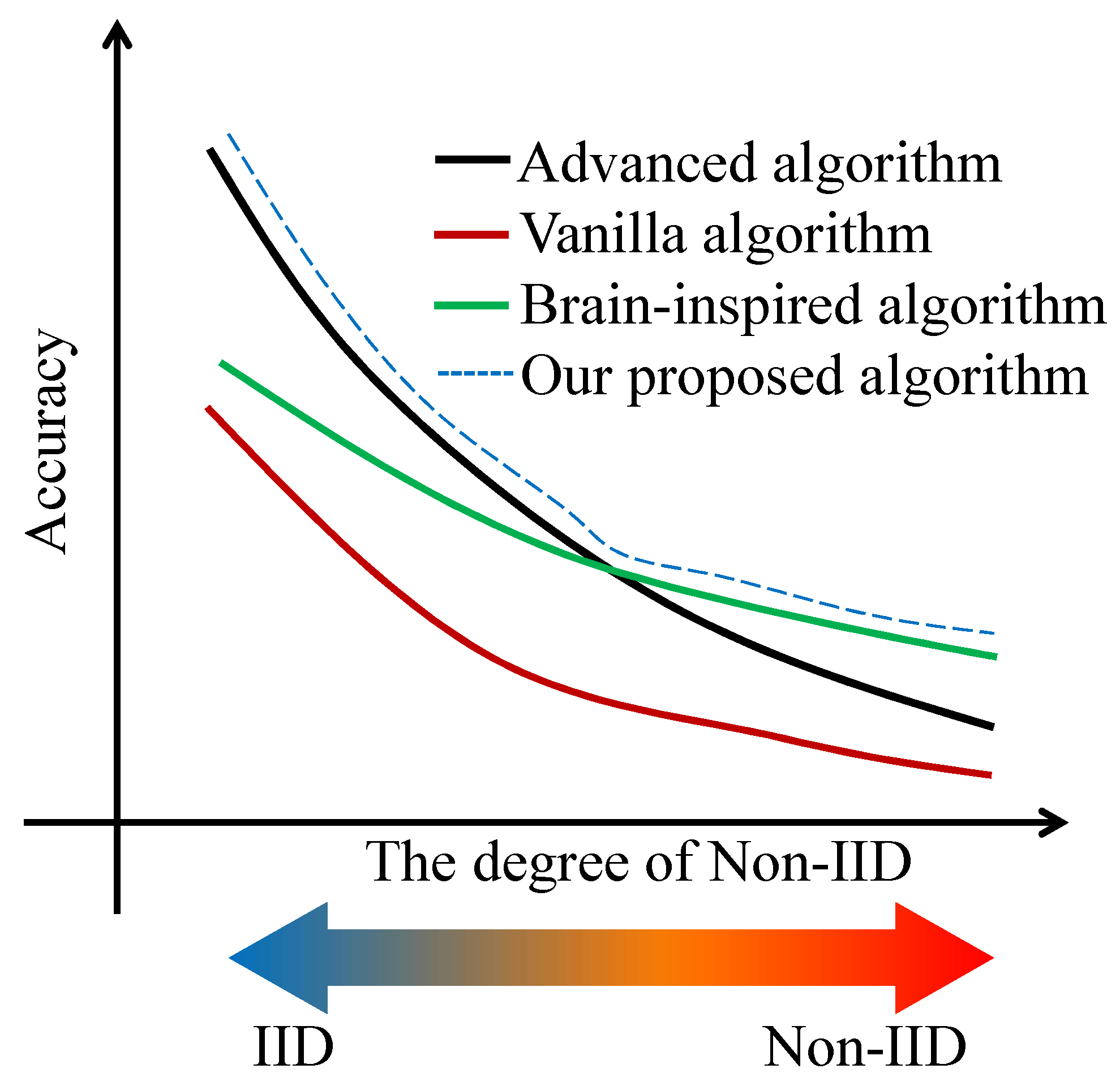
Figure 1. Testing different algorithms on different severities of non-identical datasets.
Information 16 00861 g001
Figure 2. Architecture of federated learning. Different colors and shapes represent different distribution of data.
Information 16 00861 g002
Figure 3. Distribution of class sample quantities. The whole dataset is partitioned into 10 clients. (Left) Under severe Non-IID, there are substantial differences among clients in both data volume and inter-class distribution. (Center) Under mild Non-IID, the degree of heterogeneity is reduced. (Right) Under IID, there are no significant differences in data volume or class distribution across clients.
Information 16 00861 g003
Figure 4. An example of client distribution under different Non-IID settings is shown. The dataset contains three classes labeled c 1 , c 2 , and c 3 . The red dots denote the samples, and their locations represent the ratios of the classes. (a) IID scenario: All clients are located near the center of the triangle. Each coordinate of a sample, e.g., x 1 ( 0.34 , 0.31 , 0.35 ) , denotes the proportion of each class in the local dataset, with the sum of the values equal to 1. This indicates that each local dataset contains samples from all classes in roughly equal proportions. (b) Mild Non-IID scenario: Clients are uniformly distributed across the triangle. Some clients remain near the center, while others are located closer to the edges, reflecting moderate variations in class proportions. (c) Severe Non-IID scenario: All clients are clustered in a small corner of the triangle. For example, x 2 ( 0.02 , 0.09 , 0.89 ) indicates that a sample from class c 3 accounts for 89% of the dataset, leading to a highly imbalanced distribution.
Information 16 00861 g004
Figure 5. An illustration of the populations under different Non-IID settings. The figure is derived from the x and y coordinates in Figure 4, while the vertical axis represents the number of clients. The yellow color indicates a higher sample density in this region, while darker colors indicate a lower sample density. (a) The population under the IID setting. (b) The population under the mild Non-IID setting. (c) The population under the severe Non-IID setting.
Information 16 00861 g005
Figure 6. Comparison between the MAP estimate and the true value. The horizontal axis represents the number of samples, and the vertical axis shows the variation in the predicted values, which is illustrated using error bars. The red line indicates true value. The parameters of the Gamma function are set with a = 1 2 ,   b = 1 . (a) Severe Non-IID ( β = 0.01 ). (b) Mild Non-IID ( β = 0.1 ). (c) IID ( β = 10 ).
Information 16 00861 g006
Figure 7. The mappings between β and μ .
Information 16 00861 g007
Figure 8. Neuromodulation of local plasticity in the brain. Major neuromodulators, such as dopamine and serotonin, released from the ventral tegmental area (VTA) and the dorsal raphe nucleus (DRN), play essential roles in memory formation and the acquisition of new skills.
Information 16 00861 g008
Figure 9. Diagram of the brain-inspired algorithm. Global modulation (red solid line) influences the weight updates during gradient backpropagation (green dashed line) during local update in the client. The red lines denote the positive weight while the blue lines denote the negative weights.
Information 16 00861 g009
Figure 10. Evaluation results on MNIST under varying degrees of Non-IID and different client sampling ratios are presented. Subplots within the same column correspond to experiments conducted with client sampling ratios C = 0.2 , 0.5 , 1 , while subplots within the same row correspond to settings with different degrees of Non-IID, namely IID, mild Non-IID, and severe Non-IID, respectively.
Information 16 00861 g010
Figure 11. Evaluations on CIFAR10 over different degrees of Non-IID and sampling ratios. The subplots in the same column represent setting t with client sampling ratio C = { 0.2 , 0.5 , 1.0 } . The subplots in the same row represent the setting with different degrees of Non-IID, namely IID, mild Non-IID and severe Non-IID, respectively.
Information 16 00861 g011
Table 1. Top-1 accuracy. Bold values indicate the highest performance among all methods under the same experimental setting.
MNISTCIFAR10
C = 0.2 C = 0.5 C = 1 C = 0.2 C = 0.5 C = 1
Severe
Non-IID
FedNACA84.09 ± 0.6884.69 ± 0.4184.48 ± 0.2242.88 ± 0.8357.76 ± 0.6358.16 ± 0.45
Proposal84.65 ± 0.7891.99 ± 0.3891.54 ± 0.257.42 ± 0.6858.22 ± 0.6159.21 ± 0.32
FedAvg71.02 ± 0.7689.96 ± 0.6990.86 ± 0.3822.38 ± 1.2125.33 ± 0.9826.37 ± 0.55
FedProx78.17 ± 1.0264.53 ± 0.8862.88 ± 0.6525.96 ± 1.1230.35 ± 0.9430.61  ± 0.89
MOON45.59 ± 1.4153.17 ± 0.953.69 ± 0.8923.89 ± 1.6627.54 ± 1.3229.44 ± 1.2
SCAFFOLD88.84 ± 0.8488.69 ± 0.789.62 ± 0.6631.35 ± 1.3133.14 ± 0.9736.39 ± 0.71
Mild
Non-IID
FedNACA82.35 ± 0.5184.65 ± 0.3185.66 ± 0.1532.72 ± 0.6833.85 ± 0.4534.48 ± 0.33
Proposal96.86 ± 0.4496.46 ± 0.396.34 ± 0.1644.23 ± 0.5347.28 ± 0.448.2 ± 0.28
FedAvg96.89 ± 0.5297.21 ± 0.2996.28 ± 0.1523.21 ± 0.6624.01 ± 0.4826.3 ± 0.25
FedProx93.86 ± 0.5293.96 ± 0.392.61 ± 0.1643.54 ± 0.744.73 ± 0.4243.9 ± 0.29
MOON94.03 ± 0.6194.58 ± 0.3492.44 ± 0.1941.27 ± 0.7343.16 ± 0.5143.16 ±  0.36
SCAFFOLD88.46 ± 0.4890.52 ± 0.3191.52 ± 0.1636.3 ± 0.6840.11 ± 0.4641.53 ±  0.31
IIDFedNACA92.72 ± 0.2292.82 ± 0.1292.75 ± 0.0928.47 ± 0.5628.61 ± 0.2934.48 ± 0.19
Proposal97.51 ± 0.297.14 ± 0.1296.97 ± 0.1141.37 ± 0.5742.88 ± 0.2843.57 ± 0.21
FedAvg97.57 ± 0.297.76 ± 0.1197.7 ± 0.133.01 ± 0.5834.76 ± 0.335.03 ± 0.22
FedProx96.34 ± 0.1996.39 ± 0.1196.42 ± 0.1148.77 ± 0.5249.43 ± 0.2649.59 ± 0.22
MOON96.46 ± 0.2595.4 ± 0.1494.28 ± 0.1346.6 ± 0.6147.52 ± 0.3346.81 ± 0.24
SCAFFOLD89.12 ± 0.2190.73 ± 0.1292.01 ± 0.1138.87 ± 0.5740.14 ± 0.3141.77 ± 0.22
Disclaimer/Publisher’s Note: The statements, opinions and data contained in all publications are solely those of the individual author(s) and contributor(s) and not of MDPI and/or the editor(s). MDPI and/or the editor(s) disclaim responsibility for any injury to people or property resulting from any ideas, methods, instructions or products referred to in the content.