Article

An Automated Domain-Agnostic and Explainable Data Quality Assurance Framework for Energy Analytics and Beyond

by
Balázs András Tolnai
,
Zhipeng Ma
,
Bo Nørregaard Jørgensen
and
Zheng Grace Ma
*
SDU Center for Energy Informatics, Maersk Mc-Kinney Moeller Institute, The Faculty of Engineering, University of Southern Denmark, 5230 Odense, Denmark
*
Author to whom correspondence should be addressed.
Information 2025, 16(10), 836; https://doi.org/10.3390/info16100836
Submission received: 19 June 2025 / Revised: 23 September 2025 / Accepted: 24 September 2025 / Published: 26 September 2025
(This article belongs to the Special Issue Artificial Intelligence and Data Science for Smart Cities)

Abstract

Nonintrusive load monitoring (NILM) relies on high-resolution sensor data to disaggregate total building energy into end-use load components, for example HVAC, ventilation, and appliances. On the ADRENALIN corpus, simple NaN handling with forward fill and mean substitution reduced average NMAE from 0.82 to 0.76 for the Bayesian baseline, from 0.71 to 0.64 for BI-LSTM, and from 0.59 to 0.53 for the Time–Frequency Mask (TFM) model, across nine buildings and four temporal resolutions. However, many NILM models still show degraded accuracy due to unresolved data-quality issues, especially missing values, timestamp irregularities, and sensor inconsistencies, a limitation underexplored in current benchmarks. This paper presents a fully automated data-quality assurance pipeline for time-series energy datasets. The pipeline performs multivariate profiling, statistical analysis, and threshold-based diagnostics to compute standardized quality metrics, which are aggregated into an interpretable Building Quality Score (BQS) that predicts NILM performance and supports dataset ranking and selection. Explainability is provided by SHAP and a lightweight large language model, which turns visual diagnostics into concise, actionable narratives. The study evaluates practical quality improvement through systematic handling of missing values, linking metric changes to downstream error reduction. Using random-forest surrogates, SHAP identifies missingness and timestamp irregularity as dominant drivers of error across models. Core contributions include the definition and validation of BQS, an interpretable scoring and explanation framework for time-series quality, and an end-to-end evaluation of how quality diagnostics affect NILM performance at scale.

1. Introduction

The increasing deployment of smart sensors and advanced metering infrastructure (AMI) has advanced energy monitoring and management in buildings [1,2]. These technologies enable data-driven strategies for efficiency, diagnostics, and predictive control. Applications such as non-intrusive load monitoring (NILM), anomaly detection, and building performance benchmarking rely on large volumes of high-frequency time-series data [3,4,5].
Data quality remains a persistent challenge [6]. Sensor faults, communication errors, missing values, and temporal inconsistencies degrade even advanced machine-learning models [7,8,9,10]. For NILM and related analytics, which rely on subtle temporal patterns and statistical relationships, degraded inputs can cause substantial disaggregation or prediction errors [11].
Prior studies report widespread issues in public building datasets. For example, over 70% of energy datasets contain long gaps, duplicated timestamps, or sensor drift [12]. Existing data-profiling tools such as Great Expectations and Deequ provide rule-based validation and anomaly detection, yet they are not designed for multivariate sensor streams or irregularly sampled time series [13,14]. Domain-specific efforts such as NILMTK focus on preprocessing for disaggregation but often assume baseline data quality [15]. Research in IoT and sensor networks explores anomaly detection with deep and statistical models, but many methods lack interpretability or general-purpose integration [16,17].
To address these limitations, this paper introduces a modular, fully automated pipeline to assess, score, and remediate data quality in time-series building datasets. The pipeline performs automated profiling, scoring, and explanation to support dataset selection, preprocessing, and model development by providing actionable insights into data reliability.
While the pipeline is generally applicable to multivariate time series, the present study focuses on NILM as a representative case to demonstrate how quality metrics correlate with model performance and to validate interpretability strategies under realistic conditions. We validate on the ADRENALIN dataset of nine buildings at multiple temporal resolutions [18,19]. Experiments show that the Building Quality Score correlates with NILM performance and that LLM-based narratives enhance user trust and decision-making in data-curation workflows.
Problem statement: NILM model performance degrades in the presence of data quality defects, including missing values, short and extended gaps, timestamp irregularities, and distributional instabilities that arise from sensor faults and operational changes.
Objective: Quantify how specific data quality defects affect NILM accuracy and introduce a validated Building Quality Score that predicts downstream performance. Specifically, measure the effects of missingness and gap structure, timestamp irregularities, and distributional instability on model error; aggregate direction-aligned metrics into completeness C, temporal regularity T, and statistical stability S; and verify that the resulting score predicts error, supports dataset ranking and remediation, and yields interpretable attributions via SHAP with concise figure-conditioned narratives.
Contributions:
  • A modular pipeline and metric set for smart-building time series.
  • A Building Quality Score with task-aligned weights for completeness, temporal regularity, and statistical stability.
  • SHAP-based sensitivity analysis that links metrics to NILM error.
  • An LLM module that converts figures into concise diagnostic narratives.
The remainder of this paper is structured as follows. Section 2 reviews prior work in data quality profiling, imputation, explainability, and LLM-based diagnostics. Section 3 presents the architecture of the proposed pipeline, detailing metric computation, scoring design, and prompt engineering strategies. Section 4 reports experimental findings on the ADRENALIN project’s dataset, evaluating metric-to-performance correlations, NaN handling. Section 5 discusses the interpretability, scalability, and limitations of the framework. Finally, Section 6 concludes with implications for future research in quality-aware analytics.

2. Related Works

Research on data quality in smart building environments intersects with several critical domains: data validation and profiling, time-series anomaly detection, machine learning for building energy systems, and missing data imputation. The following literature review highlights peer-reviewed contributions from each of these domains, selected based on verified content and relevance.

2.1. Sensor Data Quality and Validation

Sensor integrity is central to smart building analytics. In a systematic review, Ref. [6] provides a taxonomy of data quality dimensions for sensor networks, identifying key metrics such as completeness, accuracy, and timeliness that are directly applicable to building datasets. Their findings emphasize that anomalies such as data gaps and sensor drift are often unaddressed in practice.
Similarly, Ref. [20] explores end-to-end sensor pipelines in smart buildings, including data collection, storage, and validation. They conclude that robust quality control methods are essential for any data-driven application in this space.
Quality assessment systems, such as SaQC [21], introduce traceable pipelines for anomaly detection in multivariate environmental data, which can be extended to build sensor streams. The practical implications of data degradation are demonstrated in the work [22], where statistical and machine learning models exhibit reduced accuracy when exposed to corrupted input.
Recent work by [23] presents a comprehensive framework tailored to physical sensor data, extending the classic “3Vs” of big data into a 6Vs model—Volume, Variety, Velocity, Veracity, Value, and Variability. In contrast to general-purpose tools, they anchor each of these dimensions with quantitative statistical indicators, covering timestamp irregularities, format inconsistency, sampling gaps, and value instability. Their profiling pipeline not only assesses structural and semantic integrity but also suggests preprocessing actions (e.g., deduplication, resampling, imputation) based on the observed issues, directly aligning with the goals of the BQS pipeline.

2.2. Benchmark Datasets and Preprocessing for Energy Systems

Curated datasets are essential for evaluating preprocessing pipelines. The Building Data Genome Project 2 (BDG2) [24] offers hourly readings from over 1600 commercial buildings and was featured in the ASHRAE Great Energy Predictor III competition. It provides a robust baseline for resampling, aligning sensor metadata, and detecting anomalies across diverse meter types. Similarly, Liao et al.’s twenty-year campus energy dataset [25] supports long-term trend analysis and consistency checks across multiple building systems.
Recent efforts such as [26] further emphasize the importance of scale and diversity by combining simulated data from 900,000 synthetic buildings with real-world measurements from over 1900 residential and commercial sites. These benchmarks highlight the need for standardized preprocessing steps, such as gap handling, metadata normalization, and temporal alignment, when preparing datasets for modeling tasks like forecasting or disaggregation.
Recent NILM studies explicitly connect data quality to algorithmic reliability. A 2024 review notes that preprocessing is required because missing and noisy data affect load identification, and it catalogs the heterogeneity of public datasets used in NILM [27]. A methodology paper for NILM evaluation emphasizes that performance metrics depend on measurement characteristics such as sampling rate and measured quantities, and on the availability and synchronization of reliable ground truth from temporary individual-appliance measurements [28]. A comprehensive NILM survey compiles a dataset inventory and organizes approaches, highlighting gaps that motivate more systematic treatment of data conditions and benchmarking practice [4]. Complementing these observations, an imputation study targets NILM data loss and shows that tensor-completion methods can recover accuracy, underscoring the value of completeness-aware preprocessing before disaggregation [29].

2.3. Missing Data Imputation in Time Series

Handling missing values in time series is a complex challenge that significantly impacts downstream model performance. Ref. [30] provides a comprehensive review of imputation methods, ranging from classical approaches such as mean substitution and regression, to advanced techniques including K-nearest neighbors, ensemble models, and deep learning. Their analysis emphasizes the importance of aligning the method with the underlying missingness mechanism (e.g., MCAR, MAR, MNAR) and highlights the trade-offs between simplicity, accuracy, and computational complexity.
In the context of energy analytics, recent studies have proposed specialized frameworks for smart building data. Ref. [31] argues that traditional methods often fail to preserve temporal structure in energy signals, advocating for adaptive, time-aware techniques. Ref. [32] addresses this by reshaping time series into two-dimensional representations and applying partial convolution autoencoders, yielding improved performance on complex gap patterns. Ref. [33] similarly leverages deep learning, using autoencoders and temporal embeddings to reconstruct missing segments in multivariate building datasets.
Other approaches focus on capturing structural or statistical redundancy. Weber et al. [34] introduce a copy-paste strategy that fills gaps by transferring patterns observed in other sensor channels, particularly effective in repetitive usage cycles. Ref. [35] proposes a generative diffusion model that reconstructs missing regions through iterative refinement, although at a higher computational cost.

2.4. Real-Time Integrity and System Integration

As building automation evolves, maintaining data quality in real time is essential for responsive dashboards, predictive control, and automated fault detection. The paper [36] evaluates deep learning imputation methods on their latency, computational cost, and noise robustness, concluding that many RNN and CNN models, while accurate, are too heavy for real-time deployment in building systems.
Ref. [37] demonstrates a real-world, data healing pipeline in multiple European buildings, integrating continuous stream monitoring, anomaly detection, and LightGBM-based imputation to self-correct energy streams with negligible delay.
Ref. [10] provides a comprehensive review of IoT data quality dimensions, including timeliness, completeness, and consistency, and explores stream-based approaches for sliding-window completeness checks and schema enforcement, all designed to work seamlessly within high-throughput sensor environments.

2.5. Interpretable and Unified Quality Scoring

Interpretability and standardization are essential for building trust in automated quality assessment. Liguori et al. [38] introduce a physics-informed denoising autoencoder that incorporates thermal constraints into the imputation process, enabling reconstructions that are not only statistically accurate but also physically meaningful. The inclusion of domain knowledge allows users to interpret model behavior in terms of expected system dynamics.
Zhang [39] proposes a pattern-recognition-based ensemble framework that selects the most suitable imputation method for each sensor based on artificially generated gaps. This strategy yields a more robust signal reconstruction while simultaneously providing sensor-level quality insights through performance benchmarking.
Henkel et al. (2024) [40] apply SHAP-based feature attribution to building energy control systems, generating interpretable importance scores that directly reflect the contribution of input variables to each model decision. Their method bridges data-driven scoring and physical system behavior, supporting both diagnostics and control transparency.
Similarly, Peña et al. [41] introduce ShaTS, a temporal extension of SHAP that aggregates attributions across time windows. This approach produces time-aware, feature-level explanations for anomaly detection in industrial sensor networks, closely mirroring the goals of unified quality scoring in time-series pipelines.

2.6. LLM Integration and Prompt Engineering

The integration of multimodal Large Language Models (LLMs) has substantially advanced the explainability of complex systems by enabling the interpretation of heterogeneous data types, including scientific charts and tables. Leveraging state-of-the-art natural language processing capabilities, multimodal LLMs such as GPT-4o can translate intricate datasets and model outputs into coherent, human-interpretable narratives. Paper [42] represents a novel multimodal language model (LLM) specifically designed for advanced chart comprehension and generation, demonstrating a broad range of unique capabilities in this domain, ChartLlama [42] is a chart-focused multimodal model that targets chart understanding and generation with figure-to-text narration. This focus aligns with several integration patterns identified in the recent survey of LLMs for time series, which groups approaches into direct prompting, quantization, alignment with time-series encoders, vision-as-bridge inputs, and tool-augmented workflows [43].
Effective prompt engineering is crucial for fully leveraging the potential of LLMs for explainability. One prominent technique is Chain-of-Thought (CoT) prompting, which guides models to produce intermediate reasoning steps, thereby enhancing their performance on complex tasks. As demonstrated in [44], CoT prompting significantly improves LLM capabilities in arithmetic, commonsense, and symbolic reasoning tasks. Building upon this approach, the chain-of-knowledge (CoK) framework [45] dynamically incorporates grounding information from heterogeneous sources, further improving reasoning capabilities. Experimental results indicate that CoK consistently outperforms the CoT baseline in various reasoning tasks.
Translating quantitative and scientific metrics into qualitative insights is essential for enabling stakeholders to make informed decisions. LLMs have increasingly been employed to interpret complex analytical results and present them in natural language. For instance, the study in [46] has explored how LLMs can transform outputs from explainable AI techniques—such as SHAP values—into accessible narratives, providing scalable, efficient, and business-relevant explanations. The chain-of-table framework [47] introduces a multi-step tabular reasoning approach in which input tables evolve to store intermediate results, thereby improving the accuracy of table understanding. Additionally, the MultiModal Chart Assistant developed in [48] achieves state-of-the-art performance on established chart question-answering benchmarks, further demonstrating the efficacy of multimodal LLMs in complex visual data interpretation.
Figure 1 presents a bibliometric landscape derived from this paper’s bibliography. Nodes are keywords extracted from the cited articles; edges connect terms that co-occur within a citation. The map shows three clusters: data quality and validation, NILM and benchmarking, and interpretability and reporting. The proposed framework sits at their intersection by linking quality metrics to NILM error and adding SHAP attribution and concise LLM narratives.

3. Data Quality Assurance Framework

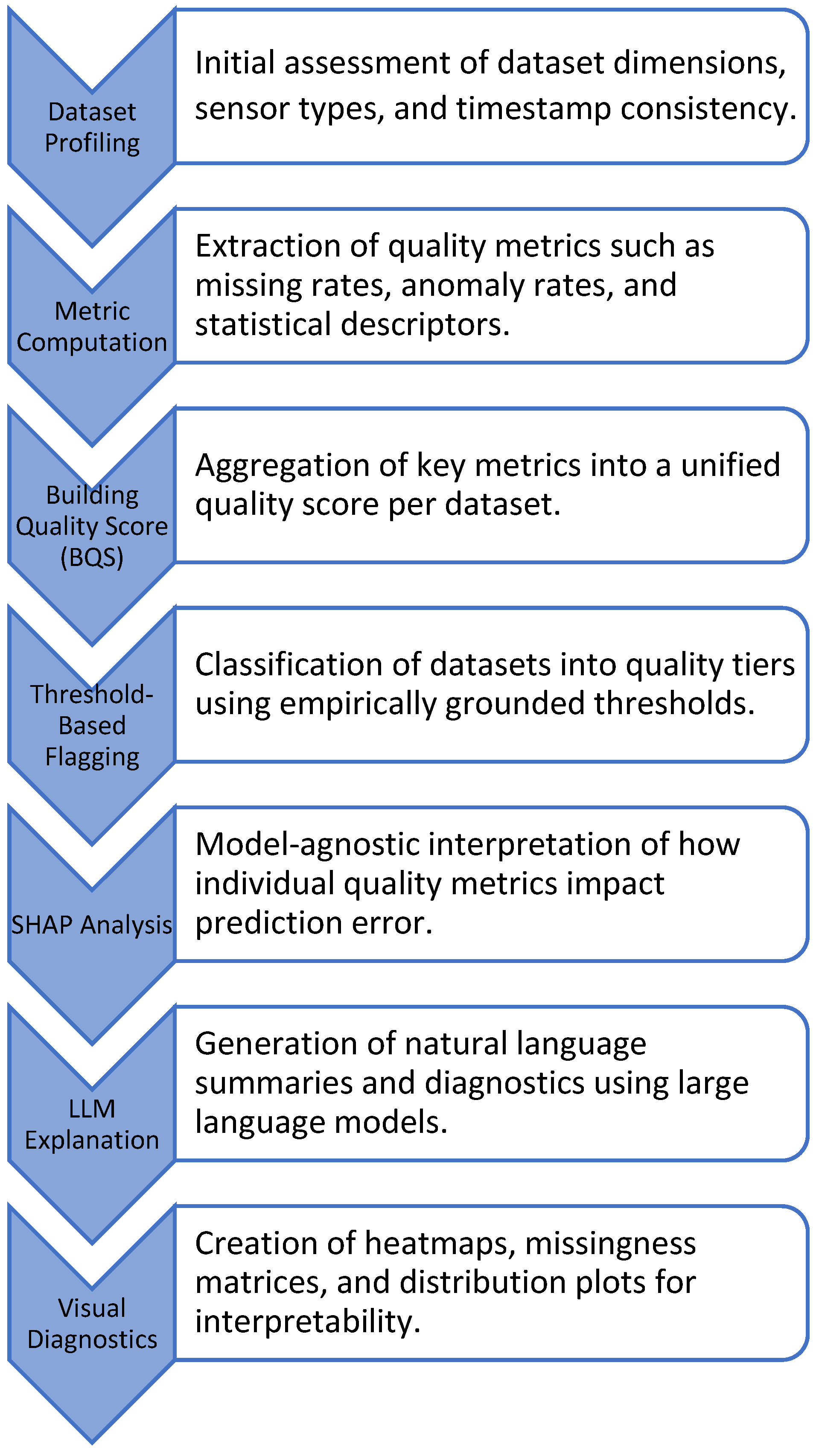
The proposed data quality assurance pipeline is modular, general-purpose, and explainable. It is designed to operate on heterogeneous time-series datasets originating from smart building sensors. The system automatically identifies and addresses data quality issues, providing human-readable insights. It comprises seven core components: (1) dataset profiling, (2) metric-based evaluation, (3) threshold-informed flagging, (4) computation of an integrated quality score, (5) SHAP-based interpretation, (6) interpretation using large language models, and (7) comparative ranking across datasets. This process is shown in Figure 2.

3.1. System Overview and Implementation

The system ingests per-building time-series files with timestamps and numeric sensor channels, aligns timezone and units, enforces strictly increasing time with de-duplication, and resamples to the analysis rate. It then computes completeness metrics such as missing_rate% and short, medium, and long gap proportions; temporal-regularity metrics such as abnormal_time_rate%, duplicate-timestamp rate, and irregular intervals; and statistical-stability metrics such as std, skewness, excess kurtosis, spike_rate%, and outlier_rate% using the rules in Section 3.2. Metric directions are aligned so larger values indicate worse quality and are converted to corpus percentile ranks. Empirical thresholds from Section 3.3 map metrics to flags and a quality tier. Percentile ranks are averaged within families to form sub-scores for completeness C, temporal regularity T, and statistical stability S, then combined as BQS = 1 − (0.50 C + 0.30 T + 0.20 S).
Baseline NILM models are evaluated with NMAE. A Random Forest surrogate is fitted from the standardized metrics to each model’s NMAE, and SHAP values quantify which metrics most affect error. For each building and resolution the outputs include the metrics table, flags and tier, C/T/S, the scalar BQS, per-model errors, SHAP summaries, and an optional LLM narrative generated zero-shot from the plots in Section 4.8, with no training performed.
The pipeline is designed for large, multi-building datasets. Core checks run in a single pass per channel with constant working memory, so throughput grows proportionally with data size. Buildings and channels are processed independently, which enables straightforward parallel execution on multi-core systems. Visual diagnostics are optional and do not affect scoring. The same routines support streaming by updating metrics incrementally with fixed memory and controllable latency.

3.2. Dataset Profiling

Each dataset is initially profiled to establish a structural and statistical baseline. This includes assessing sensor count and type, sampling intervals, temporal consistency, and the extent of value coverage. The approach is consistent with recent work advocating for the structured characterization of data in physical sensor datasets, wherein diagnostic features are grouped into spatial, temporal, and statistical dimensions to support quality assessment and remediation [23].
Sensor-type dependence is limited, but some cases can arise. The metrics assume mostly continuous, power-like channels sampled on a regular interval. Cumulative energy counters should be unwrapped before spike and outlier checks, and binary or near-binary state channels may require tailored rules because variance and step transitions differ from continuous signals.

3.3. Quality Metric Evaluation

Following profiling, a suite of standardized data quality metrics is derived for each dataset. These metrics encompass several key dimensions. First, missingness indicators capture the proportion of missing data, including both short gaps and extended periods of absence. Next, anomaly detection indicators quantify issues such as spike rate, frequency of outliers, and sudden distributional shifts that may signal sensor faults or irregular system behavior. Time-related issues are also evaluated, focusing on duplication or inconsistency in timestamps, which are known to disrupt time-series modeling and downstream analysis. Lastly, distributional characteristics such as standard deviation, skewness, and excess kurtosis are assessed for each sensor to identify irregular patterns or outliers in data distribution. These metrics serve both diagnostic and comparative purposes and are subsequently aggregated to inform a unified Building Quality Score.
Outlier and spike metrics: Outliers are identified per sensor using a robust whisker rule computed from the 20th and 80th percentiles. Let q20 and q80 denote these percentiles; the upper and lower whiskers are q80 + 2(q80 − q20) and q20 − 2(q80 − q20), respectively. Any observation above the upper whisker or below zero is counted as an outlier, and the outlier rate is reported as a percentage of non-missing samples. Spikes are sudden reversals detected on first differences: a spike is counted when two consecutive differences exceed ±2σ in opposite directions, where σ is the standard deviation of values below the upper whisker. The spike rate is likewise expressed as a percentage of non-missing samples. These rules match the implementation used to produce the metric tables and figures.
Seasonal decomposition for visual diagnostics: For interpretability figures, seasonal–trend decomposition is performed with an additive model. The seasonal period is estimated automatically from the series by FFT peak detection, then capped at most half the series length and floored at 2 to avoid degenerate settings. The resulting components (observed, trend, seasonal, residual) are plotted for human inspection and are not inputs to the BQS or to the NILM models. This matches the code path used to generate the diagnostic plots

3.4. Threshold-Based Assessment

Empirically derived thresholds are applied to translate raw metric values into actionable indicators. Thresholds were seeded from repeated intervention points systematically logged during manual cleaning across buildings and sampling rates [18].
During curation, each corrective action was logged together with the affected metric, its value at the time of intervention, and the building–frequency context. For each metric, the direction was aligned so that larger values indicate worse quality. Distributions for intervention versus non-intervention segments were compared across buildings and sampling rates. A conservative cut point was then selected from the upper tail of the intervention distribution to produce stable flags across building-frequency pairs. When several candidates were plausible, the smallest cut point that still separated the two groups and maintained a monotonic trend with downstream error in validation runs was chosen.
For example, a missing rate above 40 percent or a spike rate above 0.2 percent frequently coincided with degraded disaggregation performance. These defaults are used to assign datasets to quality tiers, for example good, moderate, and poor, and to trigger flags that inform filtering and interpretation.
Because these thresholds reflect our corpus and the judgment involved in manual cleaning, they should be treated as reasonable defaults rather than universal constants and retuned for other domains or sensing regimes. To reduce subjectivity in new deployments, thresholds can be calibrated adaptively, for example by choosing cut points that maintain a monotonic relationship between each defect metric and downstream error on a small held-out set, or by applying simple calibration methods such as quantile-based binning or isotonic mapping.

3.5. Unified Building Quality Score (BQS)

To enable a quantitative and interpretable assessment of data reliability, the various metric evaluations are consolidated into a single scalar value: the Building Quality Score (BQS). This score reflects three principal dimensions of data quality: data completeness, temporal regularity, and statistical stability. Each of these dimensions encompasses several underlying metrics, and their contributions to the final score are weighted according to their observed correlation with downstream task performance.
Missingness-related metrics are the most impactful, accounting for 50% of the final score, which reflects the strong influence of data gaps and missing segments on model accuracy. Temporal irregularities, such as duplicated or erratic timestamps, contribute 30%, capturing the disruptive effects of time-related inconsistencies on time-series modeling. The remaining 20% is attributed to statistical irregularities, including extreme skewness or high kurtosis, which indicate abnormal value distributions.
Each raw metric is cast to a unitless proportion in [0, 1] at the dataset level. Proportion-style defects, such as missing_rate% or abnormal_time_rate%, are used directly after dividing by 100 where applicable. Metrics that are not expressed as percentages, such as std, skewness, and excess kurtosis, are standardized to [0, 1] using a reference distribution computed across all building and frequency pairs, with percentile-based scaling and clipping to limit outlier leverage. All metrics are oriented so that larger values indicate worse quality. Standardized metrics are then averaged within completeness C, temporal regularity T, and statistical stability S, and the final score is computed as shown in Equation (1).
B Q S = 1 0.50 · C + 0.30 · T + 0.20 · S
In this study, C aggregates missing_rate%, missing_rate_extend%, and a short-gap proportion derived from missing_short, when available. T aggregates abnormal_time_rate% or a derived abnormal-time proportion from abnormal_time. S aggregates standard deviation (std), skewness, and excess kurtosis after standardization to [0, 1] as described above. This makes the three subcomponents directly comparable and preserves monotonicity between defect severity and subcomponent magnitude. The BQS is model-agnostic. NILM baselines are used only in the evaluation to relate BQS to downstream error and to analyze metric influence via SHAP.

3.6. SHAP-Based Model Interpretation

To quantify the influence of individual data quality metrics on model performance, SHAP (SHapley Additive exPlanations) analysis was incorporated into the evaluation pipeline. SHAP assigns importance values to input features based on their contribution to a model’s output. It provides a consistent and theoretically grounded means of interpreting feature effects across model types. In this study, accuracy is measured by normalized mean absolute error (NMAE), where lower NMAE indicates higher accuracy, and SHAP is used to assess how specific data quality characteristics affect NILM accuracy.
Surrogate regressors are trained to predict average disaggregation error from the computed quality metrics. In this study a Random Forest Regressor is fitted from standardized quality metrics to the observed average NMAE for each model family, using all building–frequency pairs in the evaluation dataset. The surrogate approximates the relationship between metrics and error so that SHAP can attribute error sensitivity to each metric in an interpretable way. Surrogates are used only for interpretation and do not replace, modify, or constrain the underlying NILM models. SHAP values are computed on the fitted surrogate using the SHAP Explainer with the background dataset.
The explanations describe the surrogate’s relationship between the metrics and error, not the internal behavior of the NILM models. Global rankings use mean absolute SHAP values, which summarize average influence but omit direction and can hide differences across buildings and sampling resolutions. Because several metrics are related, credit can be shared among correlated features according to the surrogate’s structure. These attributes should be read as directional evidence of sensitivity within the dataset.
Separate surrogates are trained for BI-LSTM, Bayesian, and Time–Frequency Mask models [19]. For a given dataset, metric, and model, a positive SHAP value indicates that the metric increases the surrogate’s predicted NMAE for that model and therefore reduces expected accuracy, while a negative value indicates the opposite. Global importance is summarized as mean absolute SHAP values and displayed as bar plots, and local attributes for representative datasets are used to generate explanatory guidance. Because the global plots use mean absolute values, the bars are nonnegative; signed SHAP values are used only in local, per-dataset explanations.
As detailed in Section 4.6, the analysis reveals consistent model sensitivity to missing data, outlier prevalence, and timestamp anomalies. These findings align with the structure of the Building Quality Score and provide additional justification for its weighting scheme. Moreover, SHAP adds model-specific interpretability that complements the BQS summary by identifying the most impactful quality factors for each architecture.

3.7. Dataset Comparison and Selection

With the above modules in place, a cross-dataset comparison is performed to support filtering and selection. Each building-frequency pair is associated with its BQS and raw metrics, allowing visual inspection via heatmaps and score distributions. Buildings can be sorted by quality, and threshold-based selection can be applied to isolate data suitable for benchmarking or training.
This comprehensive methodology enables scalable, explainable, and data-driven assessment of time-series datasets, directly supporting downstream applications in modeling and analytics.

3.8. Prompt Design and Integration

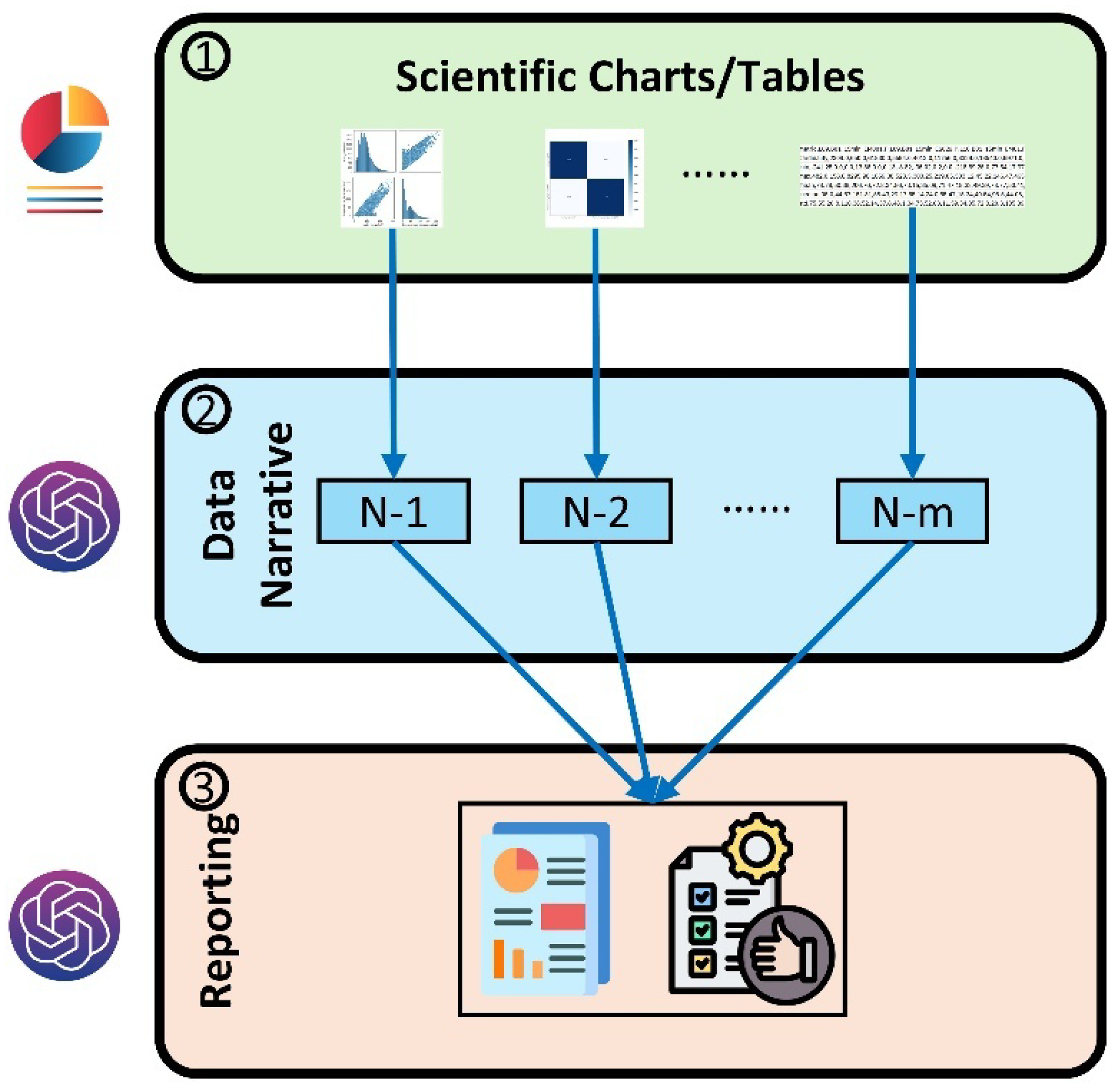
In this study, the GPT-o4-mini [49] is utilized as a multimodal large language model (LLM) to explain charts and tables for data quality assurance. As the latest lightweight model from OpenAI, it is optimized for fast and effective reasoning, offering exceptional efficiency in both coding and visual interpretation tasks. CoT prompts are utilized to guide the model in translating scientific charts and tables into human-interpretable narratives. These narratives are subsequently analyzed by the LLM to assess data quality and automatically formulate recommendations for their improvement. No model training is performed. Reports are generated by zero-shot prompting, where the chart or table image is passed to GPT-o4-mini together with the user instruction. The LLM’s role is limited to figure-conditioned narrative and report text generation, and it does not compute metrics, aggregate BQS, set thresholds, or select models.
Figure 3 presents the proposed pipeline for applying the GPT-o4-mini model to data quality assurance by interpreting scientific charts and tables. The process begins with the collection of structured data and the creation of various visualizations of it, such as scatter plots, correlation matrices, and tabular data, which serve as inputs for analysis. Using CoT prompts, the GPT-o4-mini then generates corresponding human-interpretable narratives that capture key insights, highlight patterns, and identify potential data quality issues. These narratives are subsequently synthesized into a comprehensive report that evaluates data quality and provides actionable recommendations for improvement. This end-to-end framework enables efficient, scalable, and interpretable data quality assurance, leveraging the advanced reasoning and multimodal capabilities of GPT-o4-mini.
Figure 4 illustrates the prompt design framework used to guide GPT-o4-mini in generating data narratives from scientific charts and tables. The system prompt establishes the model’s role as an expert data analyst with domain knowledge in building energy consumption, ensuring technically accurate and contextually relevant explanations. The user prompt provides a clear, structured task, instructing the model to think step by step, describe the main objects and overall scene, interpret the chart’s context, and convey the underlying message, following a predefined output template for consistency.
Figure 5 illustrates the design of the prompt for generating data quality reports. The system prompt assigns the model the role of an expert data analyst with specialized knowledge in energy consumption in buildings, capable of summarizing data quality and providing recommendations for improvement. The user prompt outlines a two-step task: first, to assess data quality based on explanations derived from scientific charts; and second, to formulate domain-specific recommendations for improving data quality, supported by detailed reasoning and analysis. This structured prompting ensures comprehensive, insightful, and actionable reporting.
Generation follows two simple steps. First, the model produces a concise narrative from each chart or table image using the prompt in Figure 3. Second, it composes a short data-quality report from those narratives using the prompt in Figure 4. Inputs are only charts and tables for the first step and the resulting narratives for the second.

4. Case Study and Results

This section presents the empirical validation of our data quality pipeline using a curated set of real-world smart building datasets used in the ADRENALIN competition [18]. Quality metrics correlation is analyzed with model performance in a NILM setting to evaluate the effectiveness of our Building Quality Score (BQS) and illustrate the impact of data quality on algorithmic success.

4.1. Dataset Overview and Evaluation Protocol

The evaluation uses the ADRENALIN competition dataset: a subset of nine smart buildings, each provided at four temporal resolutions (1-h, 30-min, 15-min, and 5-min). For each building the dataset includes the aggregate main meter series main_meter (kW) and a derived temperature_dependent (kW) series, since the competition targets temperature-dependent load disaggregation from the aggregate signal [18]. For each building-frequency pair, a complete set of quality metrics is computed using our pipeline. The results were then compared against the performance scores of 12 competition models from the ADRENALIN disaggregation challenge, and against three baseline models used in a comparative study [50], Bayesian, BI-LSTM, and Time–Frequency Mask.
Bayesian disaggregation: The baseline takes the aggregate active-power series at the analysis sampling rate as input, estimates a temperature-independent base load from mild-temperature periods, and infers a temperature-dependent thermal component via unsupervised probabilistic inference. The output is an HVAC load time series produced per building without submeter labels; the approach follows the comparative study’s formulation.
Time–Frequency Mask (TFM): The baseline operates in three stages. First, aggregate data are optionally grouped by environmental context, for example temperature regime or day type. Second, the aggregate series is transformed to the time–frequency domain using STFT and a deep model learns an Adaptive Optimal Ratio Mask as the learning target. Third, the masked spectrum is reconstructed to the time domain to yield the HVAC estimate. Inputs are STFT magnitudes of the aggregate series; the output is the reconstructed HVAC load.
BI-LSTM: The baseline consumes sequences of the aggregate series, optionally augmented with frequency-domain features to capture long-range dependencies. The architecture uses bidirectional LSTM layers followed by a dense output layer. Training uses a regression loss with standard optimization, and the output is a time-aligned HVAC load estimate.
Performance metrics reflect the normalized mean absolute error (NMAE) of each model’s disaggregated output. Lower values indicate better disaggregation performance. Quality metrics include missing rates, spike rates, outlier rates, and others derived from both raw values and statistical summaries. For each building and resolution, BQS is computed from the metric profile, then compared with NILM errors to assess how data quality relates to model performance.

4.2. Correlation Between Data Quality and Model Scores

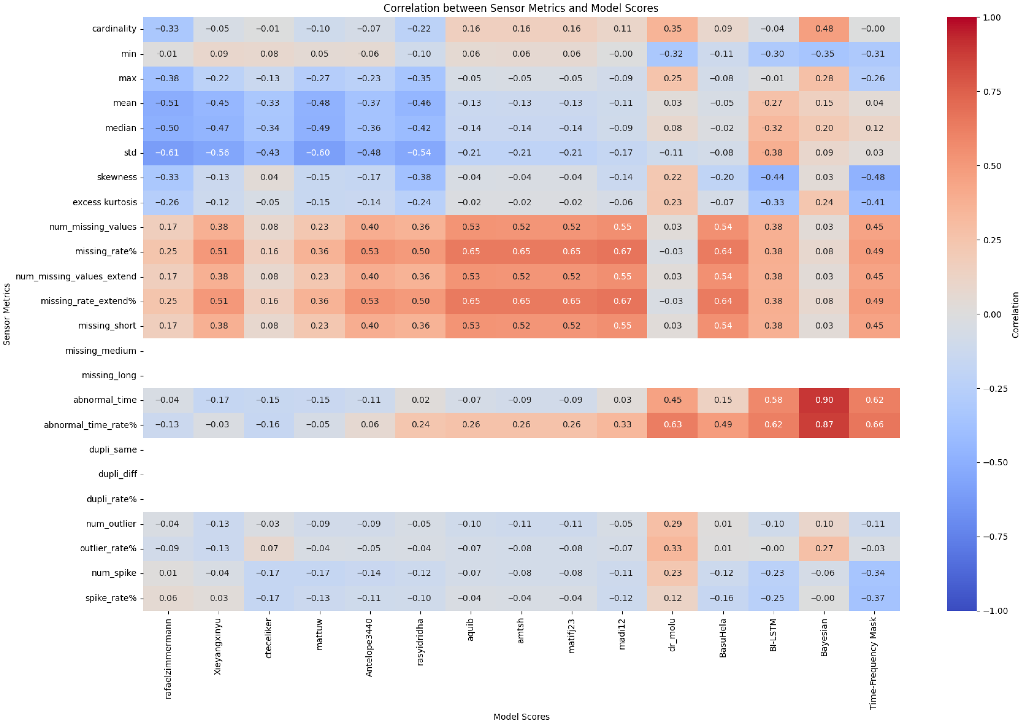
Pearson correlation coefficients were computed between each data quality metric produced by the pipeline and each model’s error (NMAE), using one value per building. A positive correlation means that larger metric values are associated with higher NMAE, hence reduced accuracy; a negative correlation means the opposite. These relationships are summarized in Figure 6, where rows are metrics, columns are NILM models, and cells are Pearson r. These are the same metrics later aggregated into the BQS, so the heatmap provides a model-specific sensitivity view that complements the scalar score.
Pearson correlations between BQS and model error were assessed as follows. Confidence intervals were obtained via the Fisher z-transform, z = arctanh (r), using standard error 1/√(n − 3), then back-transformed to r. In addition, a two-sided permutation test with 10,000 shuffles of the error labels produced a null distribution for r; the p-value equals the fraction of |r_perm| at least as large as |r_obs|. To account for testing across multiple models and metric families, Benjamini–Hochberg adjustment at q = 0.05 was applied. Effect sizes are emphasized in the main text; exact coefficients are visible in the heatmap cells, and the described procedures govern their interpretation.
Missingness metrics, including overall missing_rate% and the frequency of short and long gaps, are positively correlated with NMAE across models, indicating reduced accuracy when missingness increases. Abnormal_time_rate% shows elevated correlations for models that rely on temporal continuity, notably the BI-LSTM. Distributional statistics exhibit model-dependent effects: standard deviation, skewness, and excess kurtosis correlate more strongly for models that emphasize spectral or transient structure, and spike_rate% and outlier_rate% are especially influential in those cases. These observations align with the BQS design, which prioritizes completeness and temporal regularity while accounting for statistical stability.
Figure 7 summarizes the practical effect. BQS is on the x-axis and NMAE on the y-axis for the five models in this analysis. All fitted lines slope downward, so higher data quality aligns with lower error. A 0.1 increase in BQS corresponds to an approximate NMAE reduction of 0.06 to 0.36 for most models, and about 0.75 for one submission. In practical terms, raising BQS from 0.5 to 0.7 often lowers error by roughly 0.12 to 0.72, depending on the method. This plot complements the raw-metric heatmap by showing how the aggregated score captures the same trend at the level of building–resolution pairs.

4.3. BQS of Building L06.B01

BQS is computed solely from normalized data-quality metrics. Percent metrics are divided by 100 after aligning direction so larger values indicate worse quality. For this example, the statistical subcomponent S is mapped to 0,1 using transparent caps: s s t d   =   m i n 1 ,   C V 1.5 where C V   =   s t d m e a n ; s s k e w   =   m i n 1 ,   s k e w n e s s 2 ; and s k u r t   =   m i n 1 ,   m a x 0 ,   e x c e s s   k u r t o s i s 5 . The family means yield C, T, S, and the final score is calculated as shown in Equation (1). For this dataset the computed values are C   =   0.2571426 ,     T   =   0.0000650 ,     S   =   0.2856605 , which gives B Q S   =   0.8142771 . Dominant drivers are the completeness metrics, particularly extended missingness and short gaps. Temporal irregularities are negligible and statistical stability is moderate under the illustrative mapping. NILM outputs are not used in the BQS calculation; they are used only to study how data quality relates to downstream error.

4.4. Evaluation and Application of the Building Quality Score (BQS)

The effectiveness of the Building Quality Score (BQS) was first assessed by analyzing its correlation with average model performance across different building-frequency datasets, for which both full-quality metrics and model results were available. BQS exhibited a strong inverse correlation with normalized mean absolute error (NMAE) across nearly all NILM models, confirming that higher scores consistently reflect improved disaggregation accuracy. Buildings with BQS values above 0.85 were consistently ranked in the top quartile of model performance, whereas the three worst-performing datasets all had BQS values below 0.4 and exhibited violations across multiple quality thresholds. These results support the interpretability and predictive validity of the score.
Beyond evaluation, BQS was also tested as a filtering mechanism to guide data selection. Three threshold levels were defined to explore different tradeoffs between data quality and quantity: a strict filter (BQS > 0.85) retained only high-quality datasets and led to significant improvements in mean model accuracy, albeit with reduced coverage; a moderate filter (BQS > 0.70) offered a balance between performance gain and dataset diversity; and a lenient filter (BQS > 0.50) resulted in minimal performance improvement but maintained broader applicability. These findings indicate that BQS can be used not only to interpret data quality but also to inform preprocessing decisions that directly impact NILM model effectiveness.

4.5. Data Quality Visualization Analysis

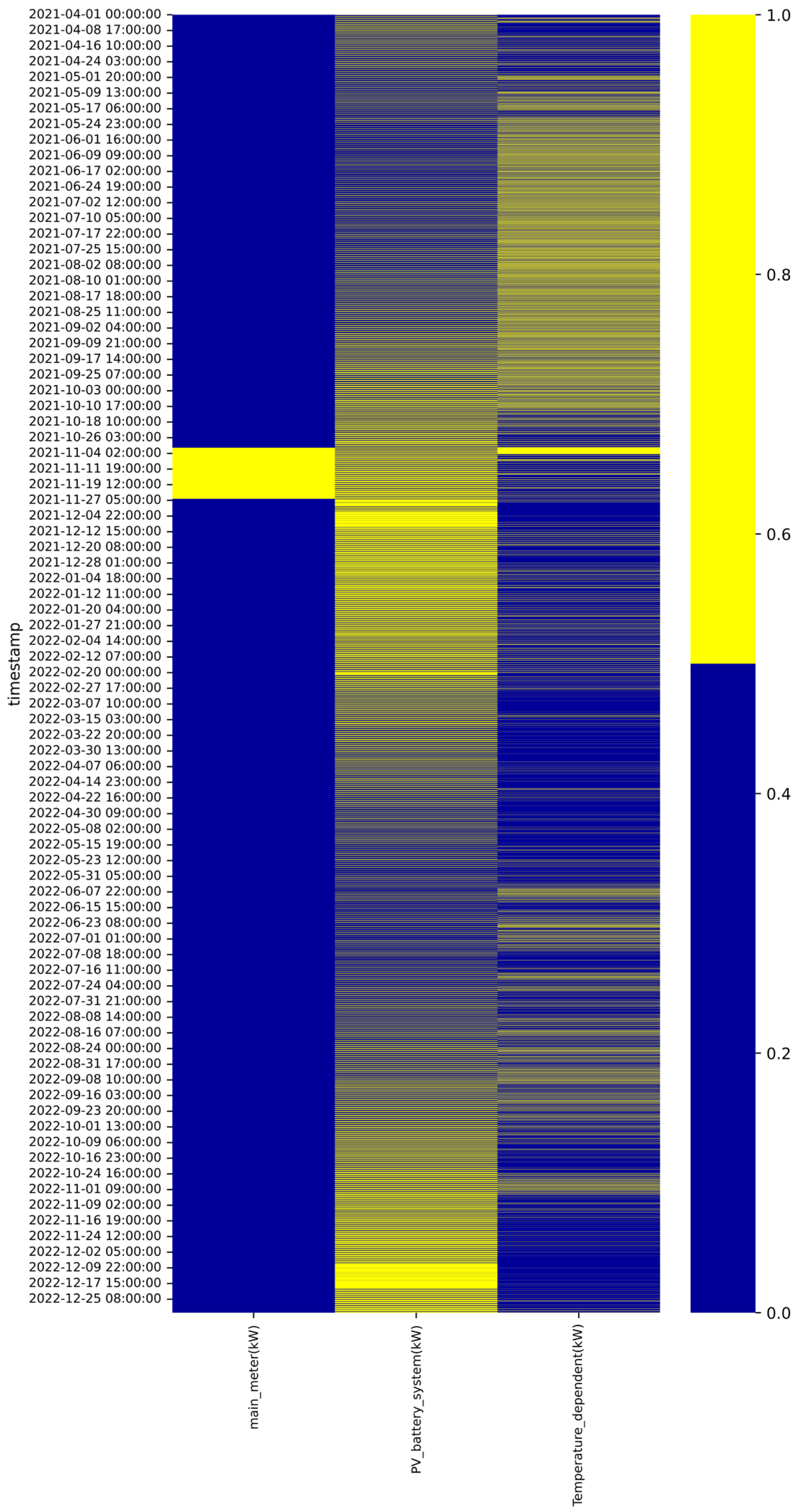
In addition to aggregated quality metrics and scores, several visualizations were generated to diagnose specific data issues across buildings. These visual tools assist in identifying missingness, statistical outliers, temporal irregularities, and inter-sensor correlations that may not be apparent from summary statistics alone. Visual diagnostics from two representative buildings, L06.B01 and L10.B01, highlight common data quality challenges and contextualize their associated BQSs. Figure 8 illustrates the missing data map for L06.B01. Prolonged periods of missingness are evident in several sensor channels, particularly during the early portion of the dataset. Such extensive gaps contribute substantially to the building’s low BQS and are likely to impair downstream modeling performance.
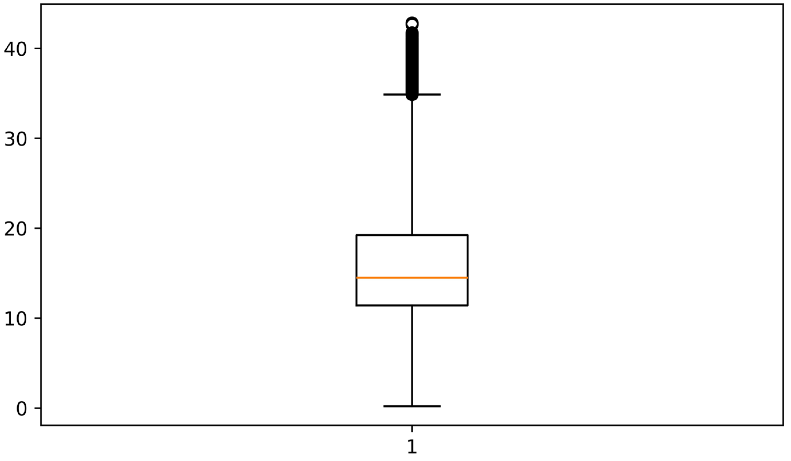
Figure 9 and Figure 10 display outlier boxplots for the main meter and temperature-dependent load respectively. While L10.B01 shows a compact interquartile range with minimal outliers (Figure 10), the L06.B01 temperature-dependent load exhibits wide variability and numerous extreme values. These observations suggest a greater presence of statistical irregularities in L06.B01, further reflected in its lower BQS.
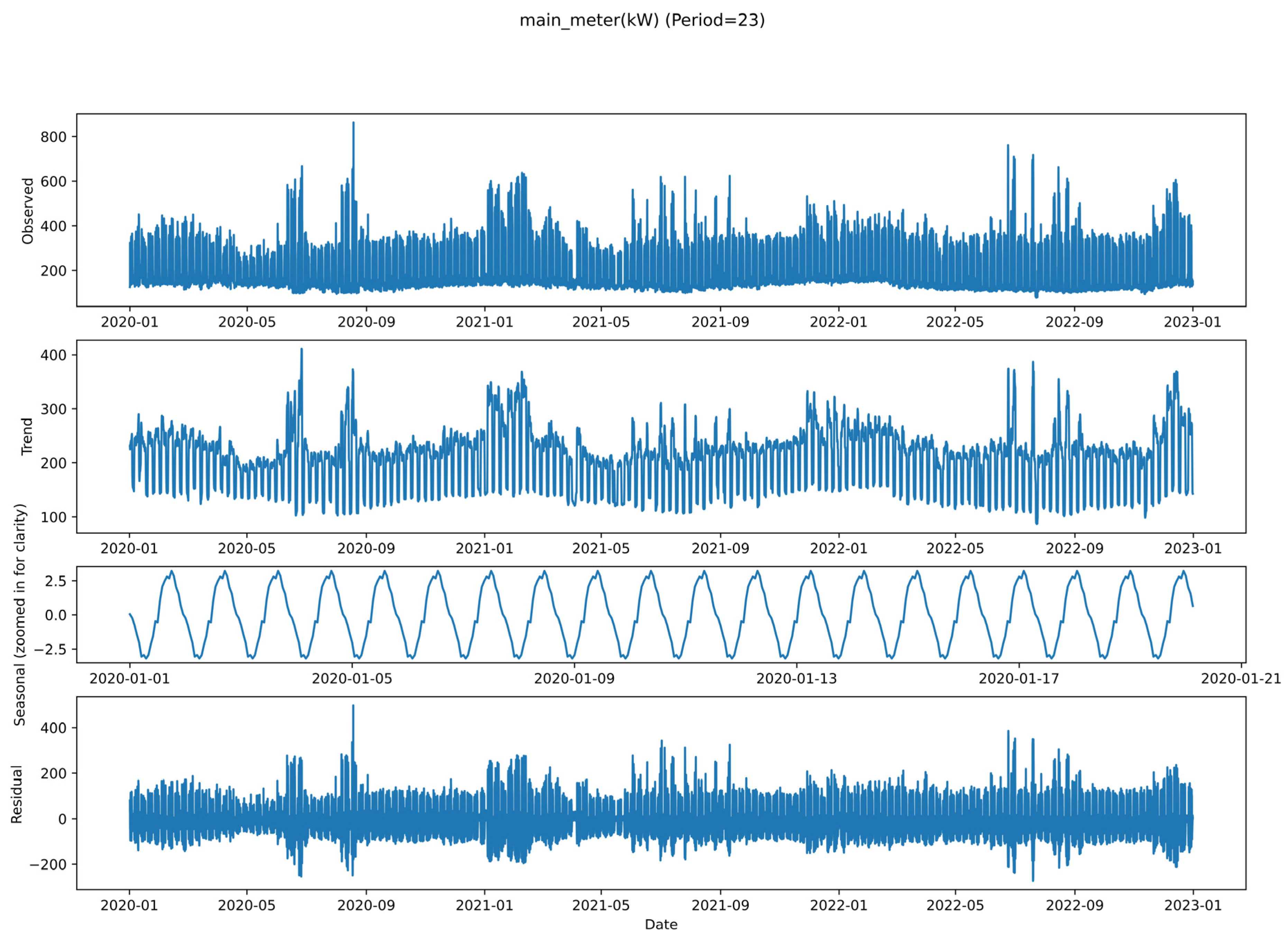
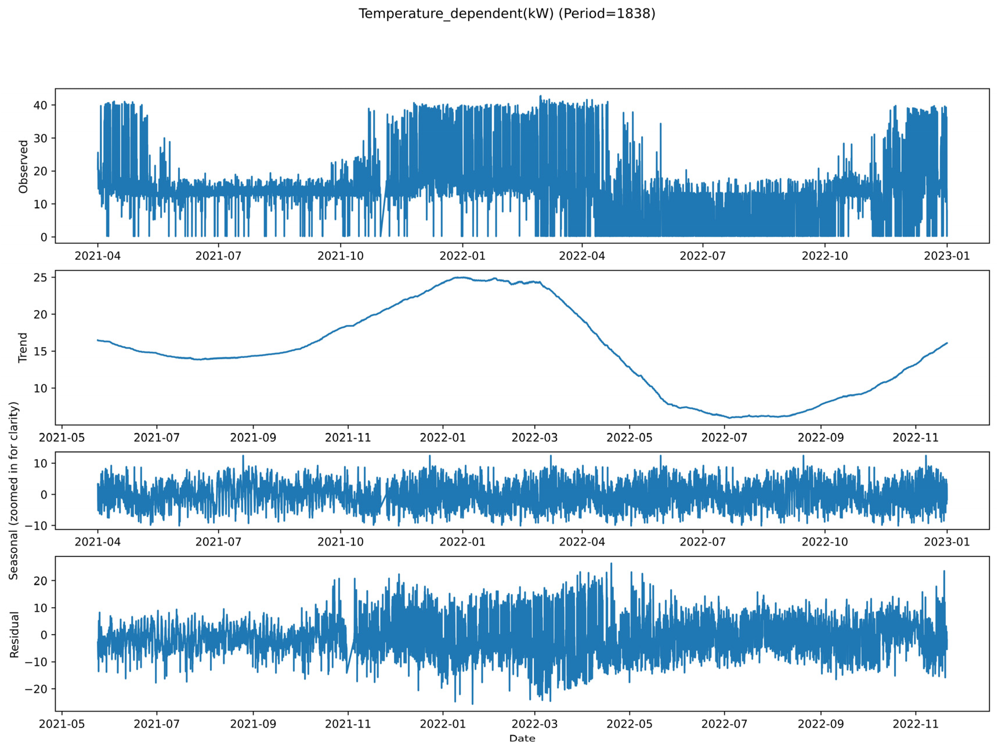
Figure 11 and Figure 12 present seasonal decompositions of the main meter and temperature-dependent load for both buildings. L10.B01’s main meter signal shows regular seasonality and a stable trend, whereas L06.B01’s temperature-dependent signal is noisy and lacks clear cyclical behavior. This absence of structure could hinder model learning and reflects low signal regularity.
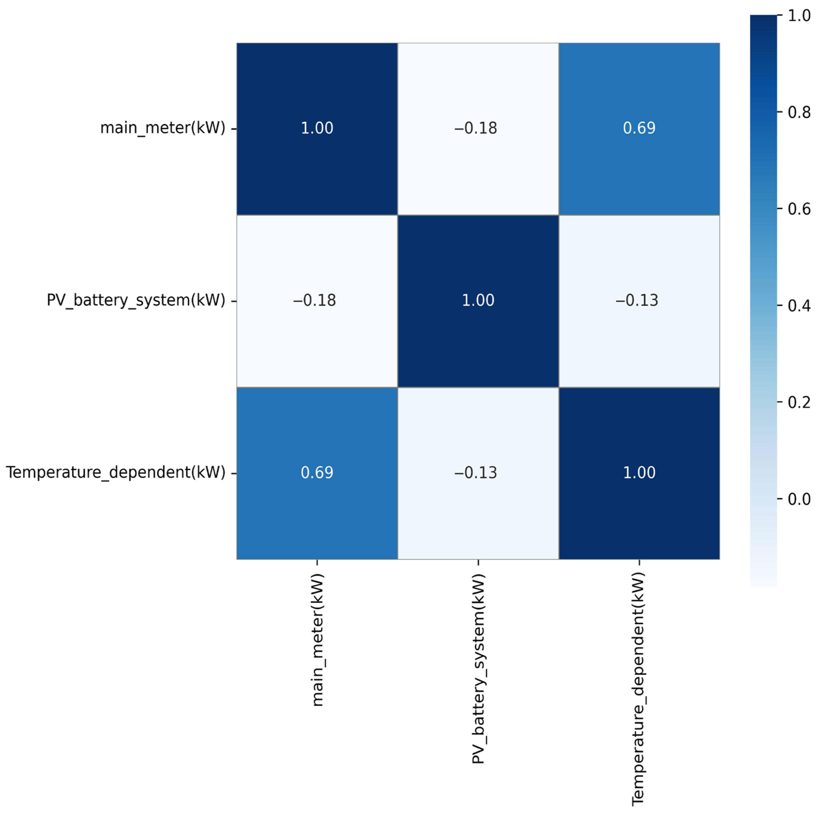
Figure 13 presents a Pearson correlation heatmap for L06.B01. PV_battery_system (kW) is positive when on-site PV or battery supplies the building and negative when the battery charges. With this convention an inverse relationship with main_meter (kW) is expected because on-site supply offsets grid import. In the example the correlation is small in magnitude, which is consistent with variable building demand dominating short-term co-variation.
Together, these visual diagnostics provide a richer understanding of individual building characteristics and validate the BQS-based quantitative assessment. They also support interpretability, enabling analysts to confirm quality issues visually and justify data selection or cleaning decisions.

4.6. Impact of NaN Handling on Quality and Performance

To estimate the potential improvements achievable through systematic handling of missing values, the effect of a simple NaN imputation strategy—using forward fill with fallback to mean imputation—was simulated across all building datasets. Following imputation, key data quality metrics were recomputed, and model performance was re-evaluated for the Bayesian, BI-LSTM, and Time–Frequency Mask algorithms. Table 1 summarizes the resulting average NMAE scores for the three selected models.
For this experiment, uniform simple imputers, for example forward fill with a mean fallback, were applied to isolate the relationship between reduced missingness and model performance while minimizing confounders. Simple methods are transparent and reproducible, they introduce few or no tunable hyperparameters, and they can be applied consistently across buildings, sampling rates, and model types. This creates a stable baseline that avoids model-specific inductive biases and enables fair comparison across NILM models. The computational cost is low, which is important when processing many building–frequency pairs. Consequently, the reported gains should be interpreted as a conservative lower bound on the improvement that can be achieved through systematic handling of missing data.
These choices have trade-offs. Simple imputers do not exploit temporal dynamics or cross-sensor structure, they may oversmooth sharp transients, and they can attenuate rare events. In the present context this is acceptable because the objective is to demonstrate that addressing missingness alone improves performance, independent of sophisticated inference about the missing values.
To contextualize the simple NaN handling used here, a controlled benchmark is specified that applies a shared masking scheme to each channel and method. Masks include short gaps (≤1 h), medium gaps (1–24 h), and long gaps (≥24 h), with MCAR and MAR patterns. Methods considered include forward fill with mean fallback, linear interpolation, seasonal naive interpolation, Kalman state-space smoothing, and K-nearest neighbors using multivariate sensors. Evaluation uses two views, data-level reconstruction error on the imputed signals, and downstream NILM error deltas after imputation. Runtime per method is measured on the same hardware.
Under this protocol, simple NaN handling serves as a conservative baseline, while seasonality-aware and model-based imputers are expected to better preserve structure in medium gaps at higher computational cost.

4.7. SHAP-Based Interpretation of Model Sensitivity

To validate the assumptions underlying the Building Quality Score (BQS), a surrogate regressor was trained to predict the average model error from the standardized data quality metrics for each NILM model family. In this study a Random Forest Regressor was fit from the metrics matrix to the observed NMAE. SHAP values were then computed on the fitted surrogate using the corpus as the background dataset. For a given dataset and metric, a positive SHAP value indicates that the metric increases predicted NMAE and therefore reduces accuracy, while a negative value indicates the opposite. Global importance is summarized as mean absolute SHAP values, so the bars shown in the figures are nonnegative. Signed values are used only for local, per-dataset explanations.
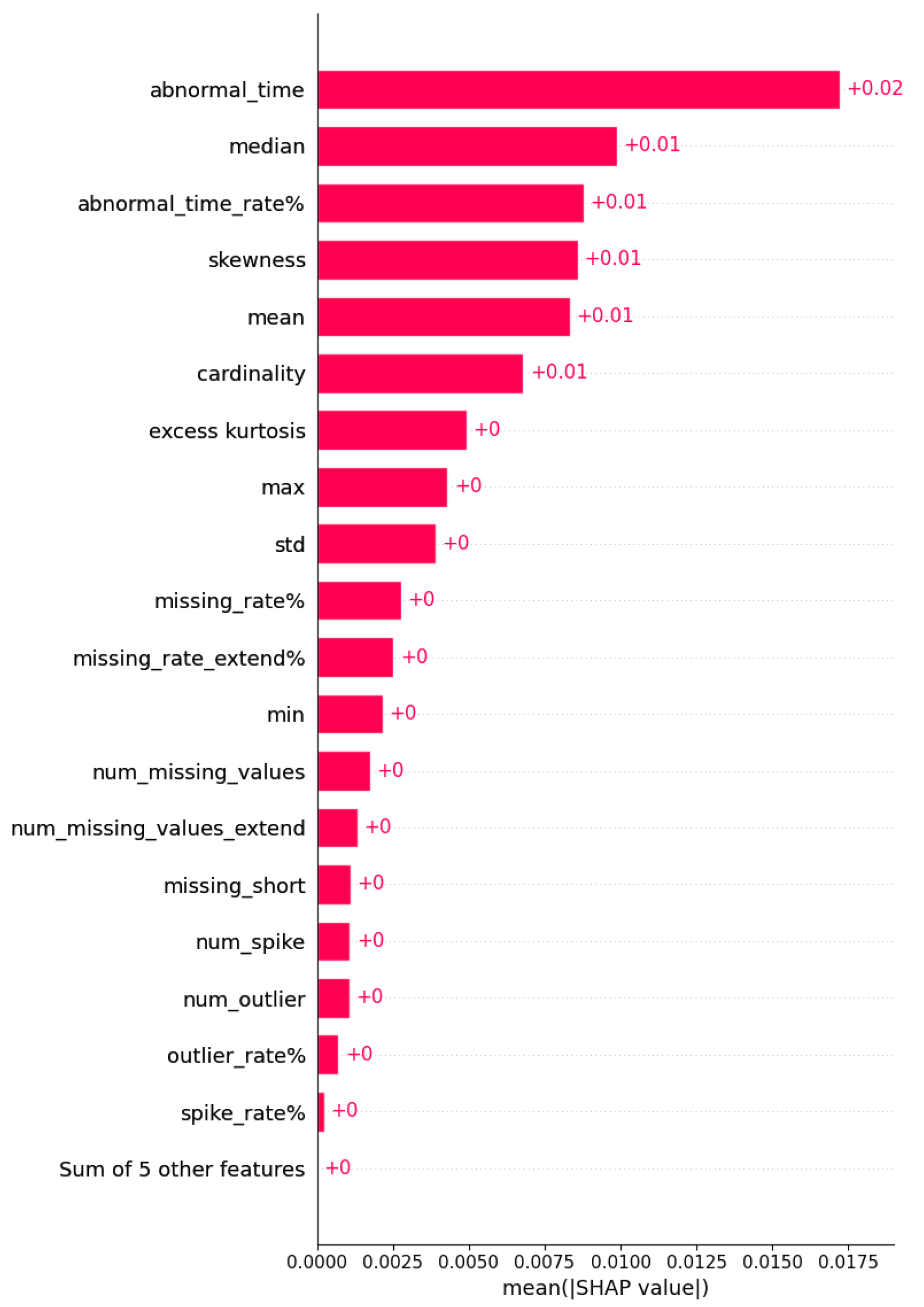
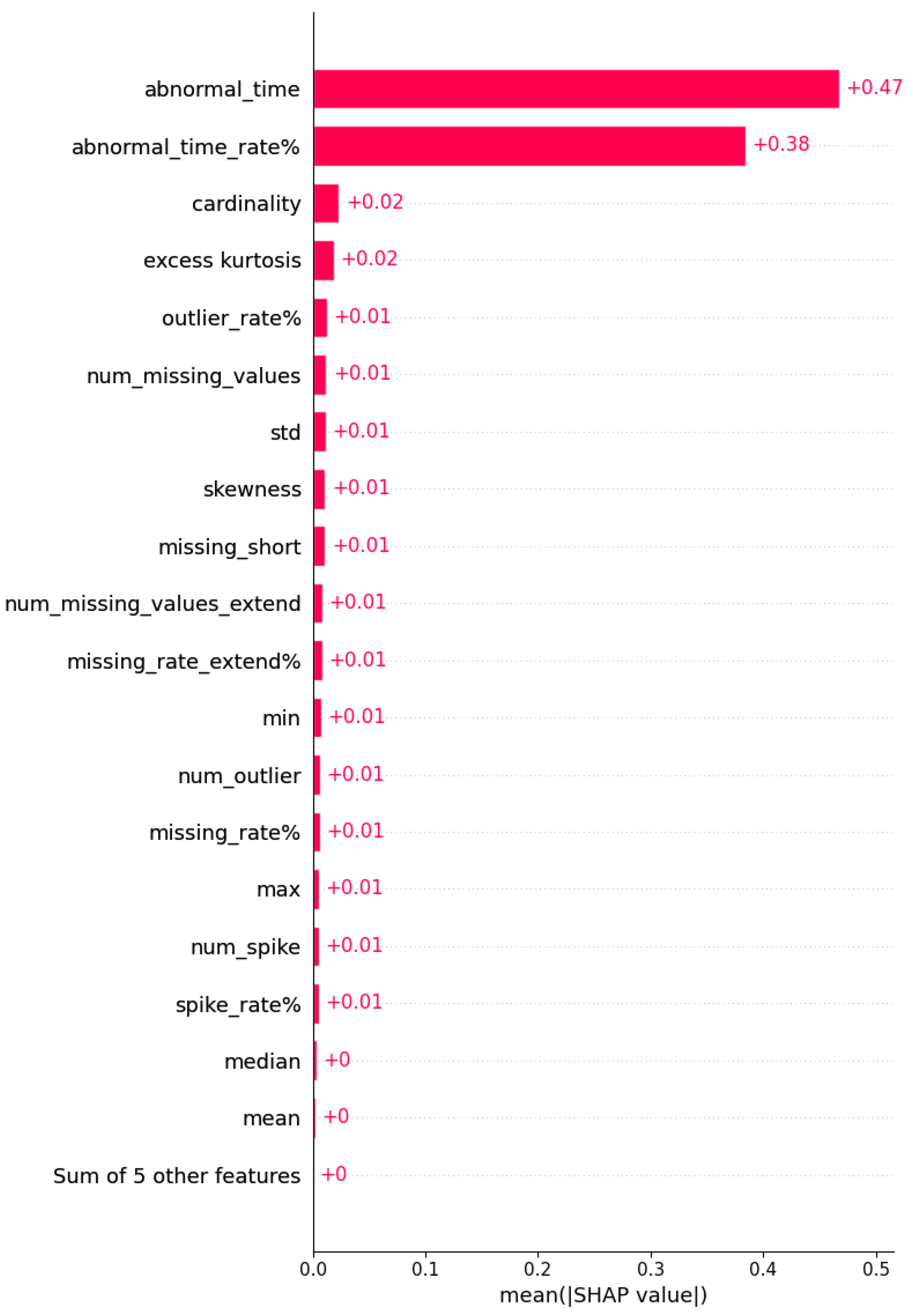
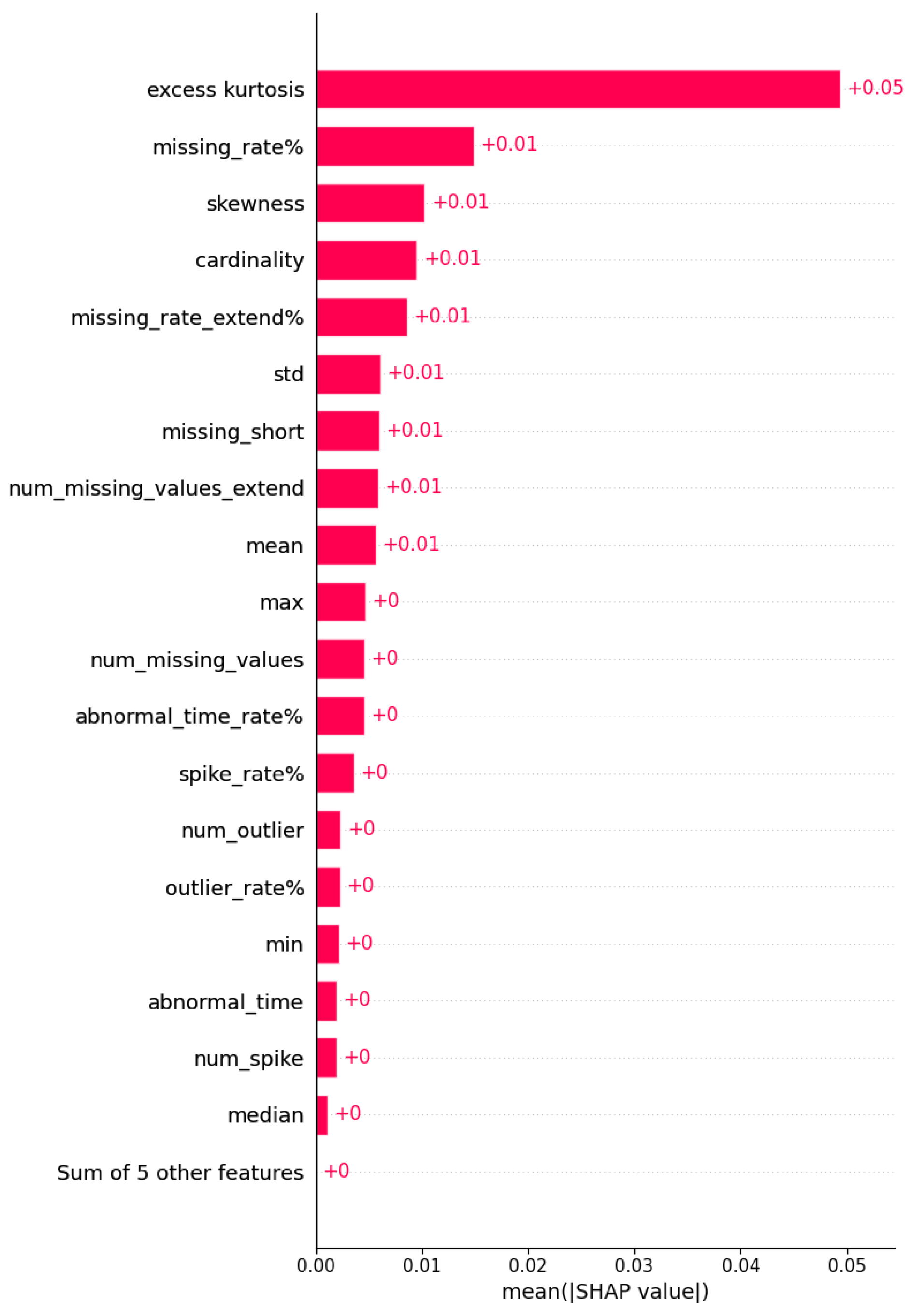
The analysis confirms that metrics associated with missing data have the highest contribution to error predictions. Metrics reflecting temporal abnormalities and statistical dispersion follow in importance. In contrast, features such as sensor cardinality and minimum or maximum value ranges show relatively minimal influence on model output. These outcomes reinforce the empirical validity and interpretability of the BQS formulation and suggest that quality-aware pipelines should prioritize mitigation of missing values and temporal inconsistencies.
Figure 14, Figure 15 and Figure 16 show mean absolute SHAP bar plots for the BI-LSTM, Bayesian, and Time–Frequency Mask models. In each case, the leading features align with missingness and abnormality-related metrics, supporting their dominant impact on performance and the proposed BQS weighting scheme.
Across models, missingness and timestamp irregularities are consistently ranked among the most critical features. This provides a strong justification for their emphasis on the Building Quality Score (BQS) formulation. Models with temporal dependencies (e.g., BI-LSTM) are especially vulnerable to incomplete or irregular sequences, while others may weight distributional anomalies more heavily.

4.8. LLM-Based Interpretability and Diagnostics

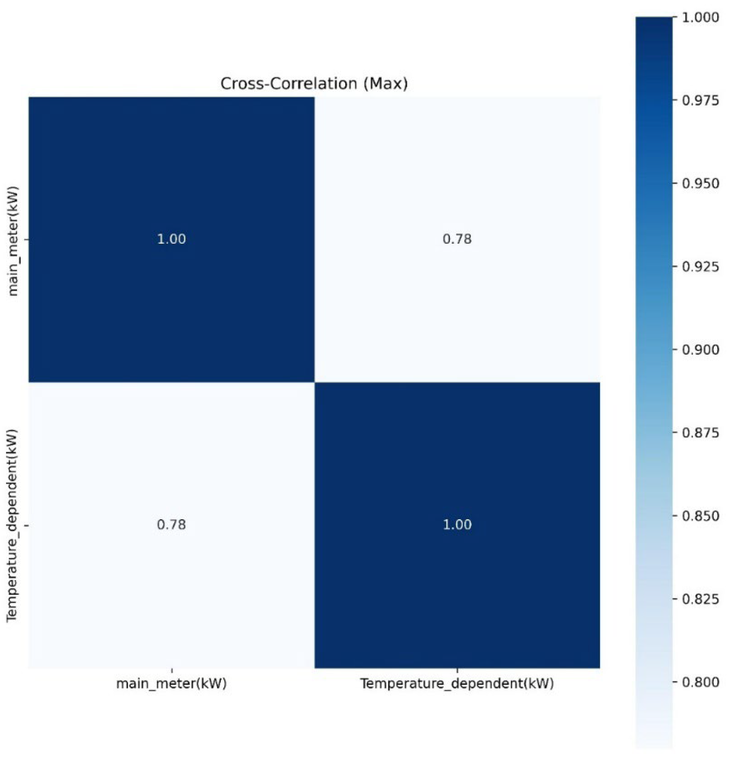
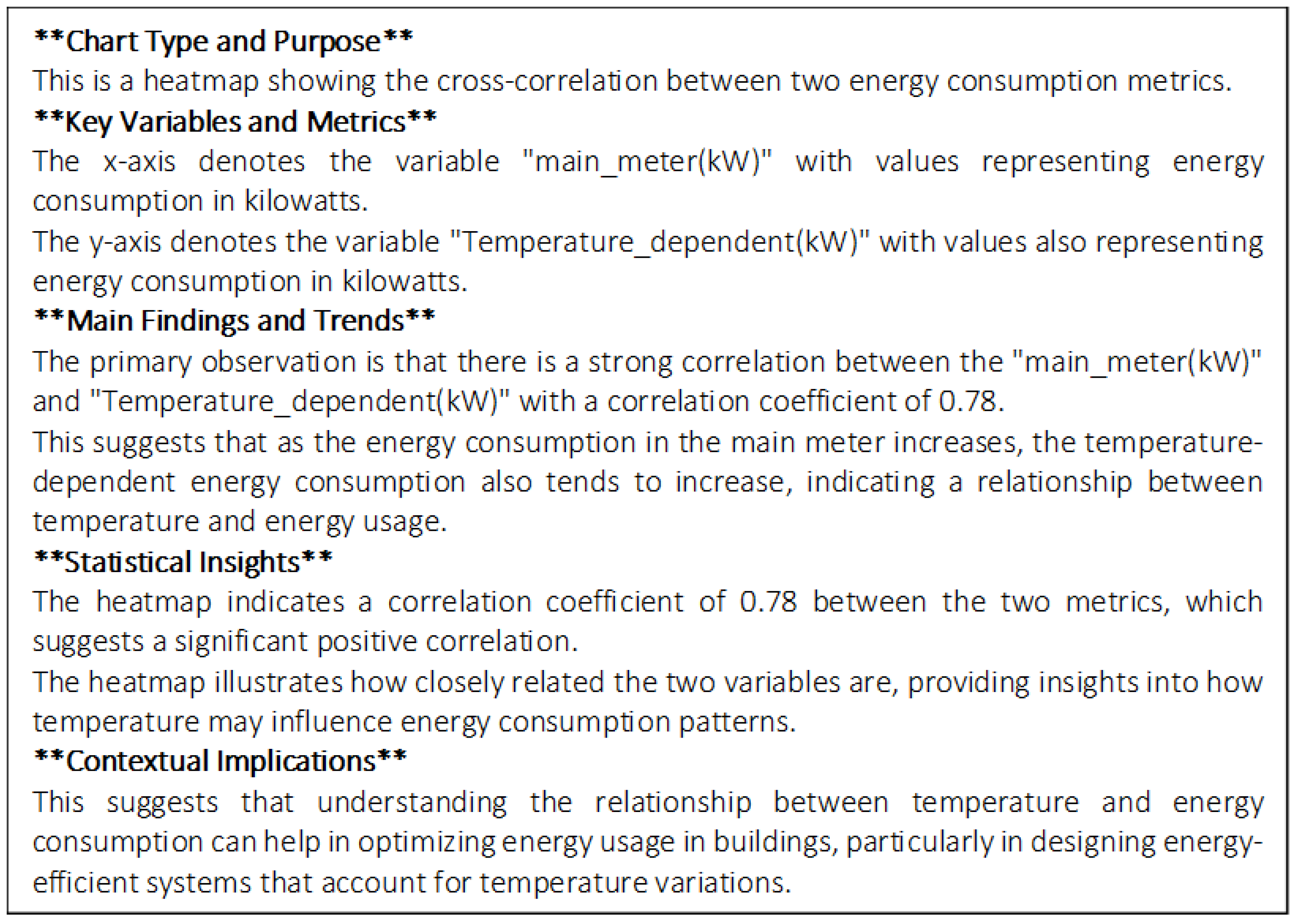
As a final validation and interpretability step, a multimodal Large Language Model (LLM), GPT-o4-mini, is used to convert the pipeline’s diagnostic visuals into human-readable guidance. The purpose of this section is to demonstrate the report-generation mechanism, not to introduce new empirical findings. Generation is zero-shot and uses only the visuals shown here. In Stage 1 the model receives a single chart or table image and produces a concise data narrative. In Stage 2 the model reads the Stage-1 narratives and composes a short data-quality report with recommendations. Two minimal examples are provided. Figure 17 and Figure 18 pair a cross-correlation heatmap between Temperature_dependent (kW) and main_meter (kW) with the generated narrative. Figure 19 and Figure 20 pair a sensor-distribution pairplot with its narrative. The examples use the ADRENALIN challenge dataset that underlies the case study. For the cross-correlation demo this dataset offers the two variables above, so the minimal pair is intentional and keeps the focus on how the LLM maps quantitative evidence to plain language. Substantive analyses of model sensitivity are reported elsewhere via the multi-metric correlation map in Section 4.2 and the SHAP results in Section 4.7.
This section presents several examples of LLM-driven diagnostics, showcasing how automated interpretation can complement statistical summaries and model-based analysis. Figure 17 and Figure 19 depict the data understanding results, while Figure 18 and Figure 20 provide the corresponding LLM-generated interpretations.
Figure 17 presents a cross-correlation heatmap, and Figure 18 provides the corresponding explanations generated by GPT-o4-mini.
Afterward, based on the scientific chart interpretations, the LLM generated high-level quality assessments and actionable suggestions using the prompts in Figure 5. Figure 21 showcases the data quality report and preprocessing suggestions of one example dataset. This is the Stage-2 report generated by zero-shot prompting of GPT-o4-mini from the Stage-1 narratives; no training or fine-tuning was performed.

5. Discussion

The results presented in the previous section underscore the strong connection between data quality and NILM model performance. This section reflects on these findings and examines their implications in the context of smart building analytics, dataset curation, and broader machine learning practices.

5.1. Comparative Positioning of Prior Work

Table 2 summarizes representative strands in the literature by methodology, typical results, and primary contributions, and contrasts them with this study’s approach. The comparison shows that most prior work treats data quality checks, benchmarking, imputation, explainability, and reporting as separate activities. In contrast, this study links quality metrics to downstream NILM error through a task-aligned score, BQS, attributes error drivers with SHAP on a surrogate model, and adds concise LLM narratives for triage.
Recent work has framed building analytics through a data-quality lens but without an operational scoring layer: the Energy and Buildings review finds fragmented, non-standard reporting and calls for consensus on requirements such as comparability and spatiotemporal granularity [12]. The present study operationalizes that gap by defining standardized metrics, aggregating them into a Building Quality Score, and showing that the score aligns with NILM error across buildings and resolutions, which the review does not quantify.
Studies that measure how missing data affects model accuracy show that imputation choice materially changes energy-time-series performance, for example LSTM mid-term load forecasting under random missingness where ML imputers outperform statistical ones [51]. The results here complement that line by linking completeness and temporal regularity metrics to observed NMAE and by demonstrating that simple, corpus-calibrated imputers reduce error across three NILM model families (Bayesian, BI-LSTM, TFM).
Broader reviews of time-series imputation in climate datasets catalog statistical, ML, and deep approaches and emphasize that method choice and data characteristics drive downstream accuracy [52]. The proposed framework situates these choices within a reproducible, interpretable pipeline in which quality diagnostics, a predictive score, and SHAP-based sensitivity provide a coherent path from data defects to expected NILM error.

5.2. Impact of Data Quality on Model Performance

The presented framework supports a more proactive and interpretable approach to data quality assurance in time-series analytics. Embedding quality assessment early in the workflow improves model reliability and generalization, reduces time spent on manual data cleaning, and enables reproducibility and cross-dataset benchmarking. This work provides both a practical toolkit and a conceptual foundation for building quality-aware machine learning systems.
In line with the quality tier thresholds proposed in earlier sections, the following usage guidelines are recommended. Datasets with a BQS of 0.85 or higher should be prioritized for benchmarking, model validation, and inclusion in training sets. Those with BQS values between 0.70 and 0.85 may still be usable, particularly if specific models are resilient to the observed quality issues. Datasets with BQS values below 0.50 generally require extensive preprocessing or should be excluded altogether, depending on the use case.
Embedding threshold-driven diagnostics directly into dataset documentation promotes transparency and reproducibility in experimental research and supports consistent decision-making across projects.
Experimental results indicate that sensor-level deficiencies—particularly missing values and temporal inconsistencies—can significantly impair the accuracy of energy disaggregation models. The degree of performance degradation varies by model architecture, with sequence-aware models demonstrating heightened sensitivity to data quality issues. These findings underscore the importance of incorporating quality-aware preprocessing into NILM pipelines.
Analysis across the nine ADRENALIN buildings revealed consistent patterns in how data quality influences model outcomes. Buildings such as L14.B03 and L14.B02, which achieved the highest Building Quality Scores (BQS > 0.98), consistently ranked among the top-performing datasets across all models. In contrast, buildings like L06.B01 and L03.B02 showed substantially lower BQSs and correspondingly elevated disaggregation errors.
These findings are broadly consistent with prior literature emphasizing the critical role of data quality in time-series learning. For instance, Refs. [12,19] reported that missing data and temporal inconsistencies significantly impair energy model reliability, matching the strong correlations observed here between BQS and model performance. Similarly, Ref. [31] highlights the vulnerability of RNN-based architectures to irregular inputs, which supports the observation that BI-LSTM performs worst on low-BQS datasets. Ref. [6] further underscores the need for comprehensive treatment of sensor degradation, categorizing key sources of quality loss such as drift, latency, and completeness, dimensions that are operationalized within the BQS scoring scheme. In line with this, Ref. [11] demonstrates that imputation performance is heavily influenced by the pattern and extent of data gaps in smart meter datasets, reinforcing the emphasis on data-specific diagnostics.
While existing studies often address data quality challenges in isolation, the present work differs by integrating these dimensions into a holistic and validated scoring framework. Notably, Ref. [33] proposes a real-time data healing pipeline tested across multiple smart buildings, but it does not explicitly link quality corrections to downstream model sensitivity. In contrast, the BQS framework not only combines integrity checks, outlier detection, and missingness, but also empirically demonstrates how these subscores predict model degradation through SHAP-based analysis, offering both diagnostic and predictive value.
A consistent pattern was observed: increased levels of missingness were strongly correlated with reduced model performance across nearly all evaluated models. This highlights the importance of developing effective strategies for handling missing data during preprocessing. While basic methods such as deletion or linear interpolation are commonly used, future investigations should consider more advanced, model-specific imputation techniques that account for temporal structure and context.

5.3. Validity of the BQS Framework

The BQS metric offers a compact yet interpretable signal of overall data usability. Its ability to predict model success, as demonstrated by its inverse correlation with average error rates, validates the subscore aggregation framework. Even simple linear weightings, informed by empirical analysis, yield a powerful summary of complex, multidimensional quality characteristics.
Beyond NILM, the methodology adapts with minimal changes. The same workflow applies: profiling, metric computation and standardization, threshold-informed flagging, surrogate-regressor fitting for SHAP, and scalar scoring. For short-term load forecasting, temporal regularity should carry more weight, with added metrics for calendar coverage consistency and stability of diurnal patterns, and thresholds calibrated on a small held-out set. For fault detection and diagnostics, statistical stability should carry more weight, with added metrics such as spike rate with run-length statistics, change-point frequency, and cross-sensor balance checks for related meters. For PV and DER analysis, temporal regularity and sensor coherence matter, with added metrics for irradiance–power alignment, clear-sky consistency, night-time zero validation, and ramp-rate plausibility. Subcomponent weights are rebalanced to the target task’s sensitivity profile, and thresholds are initialized from defaults and then calibrated to the new corpus.

5.4. Interpretability and Explainability in Quality Assessment

The integration of large language models into the pipeline introduces a new layer of interpretability that bridges raw metrics and human reasoning. Instead of relying solely on tabular diagnostics, users receive tailored feedback that translates statistical red flags into intuitive explanations and action plans.
This capability is particularly valuable for interdisciplinary collaboration, where non-technical stakeholders (e.g., building operators, policymakers) may need to understand the rationale behind dataset selection or exclusion.
Table 3 summarizes practical properties of commonly used imputers for building sensor data. It is method-focused and does not require numerical.

5.5. Cross-Domain Applicability

Although the evaluation focuses on NILM, the framework is task agnostic because the Building Quality Score decomposes quality into completeness C, temporal regularity T, and statistical stability S. These components describe failure modes that recur in most time-series settings and can be used to gate data, rank datasets, and set quality-aware thresholds before modeling.
Quality tiers transfer naturally to adjacent domains. In forecasting, C anticipates gap sensitivity, T reflects sampling stability that affects seasonality extraction, and S flags distributional skew or heavy tails that degrade extrapolation. In fault and anomaly detection for IoT or industrial telemetry, S captures event-like spikes while T protects against timestamp irregularities that create false triggers. In healthcare wearables, C summarizes adherence, T summarizes logging regularity, and S highlights motion artifacts that bias inference. In EV charging and mobility analytics, C and T screen sessions for missing segments or meter misalignment and S helps separate stable baseload from event-driven usage. Financial and operational telemetry benefit similarly, with T ensuring ordering and sampling uniformity and S signaling regime shifts that warrant model review.
The implementation is unchanged outside NILM. Metric computation and BQS aggregation remain identical. The only adaptation is the downstream target used for SHAP attribution so that explanations refer to task-specific error. The same tiering and the same short LLM narratives can be reused to support triage and monitoring across domains.

6. Conclusions

This paper presents a comprehensive, fully automated, explainable data quality pipeline for time-series building datasets, evaluated on real-world NILM tasks and with potential for other smart-building analytics. The Building Quality Score (BQS) provides a unified and interpretable metric that consolidates missingness, outliers, and timestamp integrity into a single value predictive of model performance. This score supports a systematic approach to selecting and cleaning building datasets based on their expected impact on downstream tasks.
To interpret and validate the relationship between data quality and model outcomes, SHAP-based analysis was conducted across multiple NILM models. This enabled the identification of specific quality metrics that most influence prediction error for each architecture. The resulting insights confirm and extend the rationale behind the BQS weighting scheme, revealing consistent sensitivity patterns and model-specific dependencies. A lightweight LLM-based diagnostic module was also introduced to convert sensor visualizations and quality statistics into concise natural-language summaries, facilitating human-in-the-loop decision making.
Key components therefore include the BQS metric, SHAP-based interpretation, and an LLM-based reporting module, along with dataset filtering strategies validated on NILM tasks. Scientifically, the work formalizes a multidimensional quality scoring framework grounded in empirical model sensitivity, validates its predictive utility using SHAP analysis, and demonstrates its role in cross-dataset benchmarking and transparent data curation. These contributions enable reproducible evaluation and performance-aware preprocessing, establish a foundation for adaptive NILM deployments capable of reasoning about input quality.
While the approach demonstrates strong practical value, several limitations merit emphasis. Manually set thresholds and soft caps, although grounded in empirical evidence, may not transfer across domains, sensor mixes, sampling rates, or climates. When adapting to a new dataset, thresholds should be calibrated on a small validation subset by sweeping candidate cut points, preserving a monotonic relationship between BQS and held-out error, and constraining flag rates to avoid excessive positives on high-quality data. Caps used for statistical stability should limit the influence of heavy tails and extreme skew, with a short sensitivity analysis reporting chosen values and their effect on score stability. Fixed BQS weights reflect task emphasis and may need retuning when quality risks differ.
Attribution and reporting introduce method-specific caveats. SHAP explanations summarize a surrogate and can be unstable under correlated metrics, so global importances are best read as mean absolute values, with signed values reserved for local examples. Language-model narratives are assistive summaries of diagnostics and should not replace quantitative checks or operator review.
Results are reported in batch mode. Streaming deployments would introduce stateful gap detection, timestamp repair, and latency budgets that may require incremental variants of the metrics and different thresholds.
Reproducible use depends on versioned configurations, logged seeds, and published threshold files so that scores and flags can be audited across runs and datasets.
Future work includes cross-domain validation. Thresholds, caps, and BQS weights should be re-calibrated for additional public datasets and sensing regimes, with release of versioned configurations and threshold files to support external replication. Transfer should be tested across buildings, sampling resolutions, and climates to establish generality.
Future directions could include end-to-end learning. Fixed BQS weights and caps can be replaced with learned parameters optimized against downstream error, using a differentiable surrogate that maps quality metrics to expected loss under nonnegativity and simplex constraints. Study design should include ablations by metric family, cross-building cross-validation for robustness, and stability checks under correlated inputs, with mitigations such as monotonicity constraints, grouped regularization, and bootstrap confidence intervals.
If streaming becomes a target setting, the pipeline can be extended with incremental estimators for gaps, spikes, and timestamp integrity that operate with fixed-memory updates and explicit latency budgets. Throughput and alert delay should be benchmarked on the same dataset. Remediation can be evaluated under a shared masking protocol across common imputers, reporting both reconstruction error and downstream changes in model error. SHAP reporting can be extended with correlation-aware summaries, and the language model constrained to grounded, figure-conditioned narratives.
An integrated approach could also learn quality scores directly from task utility for disaggregation or forecasting, rather than evaluating data quality independently of downstream tasks. Latent issues such as sensor calibration drift and contextual anomalies, for example occupancy, are not yet captured and motivate adding semantic context to quality analysis.

Author Contributions

Conceptualization, B.A.T., Z.M., Z.G.M. and B.N.J.; methodology, B.A.T. and Z.M.; software, B.A.T. and Z.M.; validation, B.A.T.; formal analysis, B.A.T.; investigation, B.A.T.; resources, Z.G.M. and B.N.J.; data curation, B.A.T.; writing—original draft preparation, B.A.T. and Z.M.; writing—review and editing, B.A.T., Z.M., Z.G.M. and B.N.J.; visualization, B.A.T.; supervision, Z.G.M. and B.N.J.; project administration, Z.G.M. and B.N.J.; funding acquisition, Z.G.M. and B.N.J. All authors have read and agreed to the published version of the manuscript.

Funding

This paper is part of the ADRENALIN (Data-driven smart buildings: data sandbox and competition) project. Funded by the Energy Technology Development and Demonstration Programme (EUDP) in Denmark. (Case no. 64021-6025).

Institutional Review Board Statement

Not applicable.

Informed Consent Statement

Not applicable.

Data Availability Statement

The dataset is available on the Codalab page of the ADRENALIN load disaggregation competition. https://codalab.lisn.upsaclay.fr/competitions/19659 (accessed on 24 February 2025).

Conflicts of Interest

The authors declare no conflicts of interest.

Abbreviations

The following abbreviations are used in this manuscript:
NILMNon-Intrusive Load Monitoring
BQSBuilding Quality Score
LLMLarge Language Models
SHAPSHapley Additive exPlanations
NMAENormalized Mean Absolute Error
AMIAdvanced Metering Infrastructure
NILMTKNon-Intrusive Load Monitoring Tool Kit
SaQCSystem for Automated Quality Control
BI-LSTMBidirectional Long Short-Term Memory
CoTChain-of-Thought
CoKChain-of-Knowledge
NaNNot a Number (used to denote missing values in datasets)
RNNRecurrent Neural Network
CNNConvolutional Neural Network
IQRInterquartile Range
ASHRAEAmerican Society of Heating, Refrigerating and Air-Conditioning Engineers
BDG2Building Data Genome Project 2
EUDPEnergy Technology Development and Demonstration Programme
GPT-4oGenerative Pre-trained Transformer 4 Omni

References

  1. Hadri, S.; Najib, M.; Bakhouya, M.; Fakhri, Y.; El Aroussi, M.; Taifour, Z.; Gaber, J. Amismart an advanced metering infrastructure for power consumption monitoring and forecasting in smart buildings. Discov. Comput. 2025, 28, 121. [Google Scholar] [CrossRef]
  2. Wang, Y.; Chen, Q.; Hong, T.; Kang, C. Review of smart meter data analytics: Applications, methodologies, and challenges. IEEE Trans. Smart Grid 2018, 10, 3125–3148. [Google Scholar] [CrossRef]
  3. Ding, Y.; Liu, X. A comparative analysis of data-driven methods in building energy benchmarking. Energy Build. 2020, 209, 109711. [Google Scholar] [CrossRef]
  4. Liu, Y.; Wang, Y.; Ma, J. Non-Intrusive Load Monitoring in Smart Grids: A Comprehensive Review. arXiv 2024, arXiv:2403.06474. [Google Scholar] [CrossRef]
  5. Amasyali, K.; El-Gohary, N.M. A review of data-driven building energy consumption prediction studies. Renew. Sustain. Energy Rev. 2018, 81, 1192–1205. [Google Scholar] [CrossRef]
  6. Teh, H.Y.; Kempa-Liehr, A.W.; Wang, K.I.-K. Sensor data quality: A systematic review. J. Big Data 2020, 7, 11. [Google Scholar] [CrossRef]
  7. Xie, J.; Sun, L.; Zhao, Y.F. On the Data Quality and Imbalance in Machine Learning-based Design and Manufacturing—A Systematic Review. Engineering 2025, 45, 105–131. [Google Scholar] [CrossRef]
  8. Mohammed, S.; Budach, L.; Feuerpfeil, M.; Ihde, N.; Nathansen, A.; Noack, N.; Patzlaff, H.; Naumann, F.; Harmouch, H. The effects of data quality on machine learning performance on tabular data. Inf. Syst. 2025, 132, 102549. [Google Scholar] [CrossRef]
  9. Cicero, S.; Guarascio, M.; Guerrieri, A.; Mungari, S. A Deep Anomaly Detection System for IoT-Based Smart Buildings. Sensors 2023, 23, 9331. [Google Scholar] [CrossRef]
  10. Mansouri, T.; Sadeghi Moghadam, M.R.; Monshizadeh, F.; Zareravasan, A. IoT Data Quality Issues and Potential Solutions: A Literature Review. Comput. J. 2023, 66, 615–625. [Google Scholar] [CrossRef]
  11. Sartipi, A.; Delgado Fernández, J.; Potenciano Menci, S.; Magitteri, A. Bridging Smart Meter Gaps: A Benchmark of Statistical, Machine Learnin g and Time Series Foundation Models for Data Imputation. arXiv 2025, arXiv:2501.07276. [Google Scholar]
  12. Morewood, J. Building energy performance monitoring through the lens of data quality: A review. Energy Build. 2023, 279, 112701. [Google Scholar] [CrossRef]
  13. Schelter, S.; Lange, D.; Schmidt, P.; Celikel, M.; Biessmann, F.; Grafberger, A. Automating large-scale data quality verification. Proc. VLDB Endow. 2018, 11, 1781–1794. [Google Scholar] [CrossRef]
  14. Gong, A.; Campbell, J. Great Expectations. Zenodo, Mar. 2025, 19. [Google Scholar] [CrossRef]
  15. Batra, N.; Kelly, J.; Parson, O.; Dutta, H.; Knottenbelt, W.; Rogers, A.; Singh, A.; Srivastava, M. NILMTK: An open source toolkit for non-intrusive load monitoring. In Proceedings of the 5th International Conference on Future Energy Systems, Cambridge, UK, 11–13 June 2014. [Google Scholar]
  16. DeMedeiros, K.; Hendawi, A.; Alvarez, M. A Survey of AI-Based Anomaly Detection in IoT and Sensor Networks. Sensors 2023, 23, 1352. [Google Scholar] [CrossRef]
  17. Chatterjee, A.; Ahmed, B.S. IoT anomaly detection methods and applications: A survey. Internet Things 2022, 19, 100568. [Google Scholar] [CrossRef]
  18. Tolnai, B.A.; Ma, Z.G.; Jørgensen, B.N.; Sartori, I.; Pandiyan, S.V.; Amos, M.; Bengtsson, G.; Lien, S.K.; Walnum, H.T.; Hameed, A.; et al. ADRENALIN: Energy Data Preparation and Validation for HVAC Load Disaggregation in Commercial Buildings. In Nordic Energy Informatics Academy Conference 2025; Lecture Notes in Computer Science; Springer: Stockholm, Sweden, 2025. [Google Scholar]
  19. Tolnai, B.A.; Zimmermann, R.S.; Xie, Y.; Tran, N.; Çeliker, C.E.; Ma, Z.G.; Jørgensen, B.N.; Sartori, I.; Amos, M.; Bengtsson, G.; et al. Advancing Non-Intrusive Load Monitoring: Insights from the Winning Algorithms in the ADRENALIN 2024 Load Disaggregation Competition. In Nordic Energy Informatics Academy Conference 2025; Lecture Notes in Computer Science; Springer: Stockholm, Sweden, 2025. [Google Scholar]
  20. Lavrinovica, I.; Judvaitis, J.; Laksis, D.; Skromule, M.; Ozols, K. A Comprehensive Review of Sensor-Based Smart Building Monitoring and Data Gathering Techniques. Appl. Sci. 2024, 14, 10057. [Google Scholar] [CrossRef]
  21. Schmidt, L.; Schäfer, D.; Geller, J.; Lünenschloss, P.; Palm, B.; Rinke, K.; Rebmann, C.; Rode, M.; Bumberger, J. System for automated Quality Control (SaQC) to enable traceable and reproducible data streams in environmental science. Environ. Model. Softw. 2023, 169, 105809. [Google Scholar] [CrossRef]
  22. Lee, K.; Lim, H.; Hwang, J.; Lee, D. Evaluating missing data handling methods for developing building energy benchmarking models. Energy 2024, 308, 132979. [Google Scholar] [CrossRef]
  23. Ma, Z.; Jørgensen, B.N.; Ma, Z.G. A systematic data characteristic understanding framework towards physical-sensor big data challenges. J. Big Data 2024, 11, 84. [Google Scholar] [CrossRef]
  24. Miller, C.; Kathirgamanathan, A.; Picchetti, B.; Arjunan, P.; Park, J.Y.; Nagy, Z.; Raftery, P.; Hobson, B.W.; Shi, Z.; Meggers, F. The building data genome project 2, energy meter data from the ASHRAE great energy predictor III competition. Sci. Data 2020, 7, 368. [Google Scholar] [CrossRef] [PubMed]
  25. Liao, W.; Jin, X.; Ran, Y.; Xiao, F.; Gao, W.; Li, Y. A twenty-year dataset of hourly energy generation and consumption from district campus building energy systems. Sci. Data 2024, 11, 1400. [Google Scholar] [CrossRef] [PubMed]
  26. Emami, P.; Sahu, A.; Graf, P. Buildingsbench: A large-scale dataset of 900k buildings and benchmark for short-term load forecasting. Adv. Neural Inf. Process. Syst. 2023, 36, 19823–19857. [Google Scholar]
  27. Silva, M.D.; Liu, Q. A Review of NILM Applications with Machine Learning Approaches. Comput. Mater. Contin. 2024, 79, 2971–2989. [Google Scholar] [CrossRef]
  28. Maier, M.; Schramm, S. General NILM Methodology for Algorithm Parametrization, Optimization and Performance Evaluation. Buildings 2025, 15, 705. [Google Scholar] [CrossRef]
  29. Shi, D. Non-intrusive load monitoring with missing data imputation based on tensor decomposition. arXiv 2024, arXiv:2403.07012. [Google Scholar] [CrossRef]
  30. Alwateer, M.; Atlam, E.-S.; Abd El-Raouf, M.M.; Ghoneim, O.A.; Gad, I. Missing data imputation: A comprehensive review. J. Comput. Commun. 2024, 12, 53–75. [Google Scholar] [CrossRef]
  31. Ribeiro, S.M.; de Castro, C.L. Missing data in time series: A review of imputation methods and case study. In Learning and Nonlinear Models-Revista da Sociedade Brasileira de Redes Neurais-Special Issue: Time Series Analysis and Forecasting Using Computational Intelligence; Brazilian Society on Computational Intelligence: São Paulo, Brazil, 2021; Volume 19, pp. 31–46. [Google Scholar]
  32. Fu, C.; Quintana, M.; Nagy, Z.; Miller, C. Filling time-series gaps using image techniques: Multidimensional context autoencoder approach for building energy data imputation. Appl. Therm. Eng. 2024, 236, 121545. [Google Scholar] [CrossRef]
  33. Das, H.P.; Lin, Y.-W.; Agwan, U.; Spangher, L.; Devonport, A.; Yang, Y.; Drgoňa, J.; Chong, A.; Schiavon, S.; Spanos, C.J. Machine learning for smart and energy-efficient buildings. Environ. Data Sci. 2024, 3, e1. [Google Scholar] [CrossRef]
  34. Weber, M.; Turowski, M.; Çakmak, H.K.; Mikut, R.; Kühnapfel, U.; Hagenmeyer, V. Data-driven copy-paste imputation for energy time series. IEEE Trans. Smart Grid 2021, 12, 5409–5419. [Google Scholar] [CrossRef]
  35. Chen, Z.; Li, H.; Wang, F.; Zhang, O.; Xu, H.; Jiang, X.; Song, Z.; Wang, H. Rethinking the diffusion models for missing data imputation: A gradient flow perspective. Adv. Neural Inf. Process. Syst. 2024, 37, 112050–112103. [Google Scholar]
  36. Fang, C.; Wang, C. Time series data imputation: A survey on deep learning approaches. arXiv 2020, arXiv:2011.11347. [Google Scholar] [CrossRef]
  37. Stefanopoulou, A.; Michailidis, I.; Karatzinis, G.; Lepidas, G.; Boutalis, Y.S.; Kosmatopoulos, E.B. Ensuring real-time data integrity in smart building applications: A systematic end-to-end comprehensive pipeline evaluated in numerous real-life cases. Energy Build. 2025, 336, 115586. [Google Scholar] [CrossRef]
  38. Liguori, A.; Quintana, M.; Fu, C.; Miller, C.; Frisch, J.; van Treeck, C. Opening the Black Box: Towards inherently interpretable energy data imputation models using building physics insight. Energy Build. 2024, 310, 114071. [Google Scholar] [CrossRef]
  39. Zhang, L. A pattern-recognition-based ensemble data imputation framework for sensors from building energy systems. Sensors 2020, 20, 5947. [Google Scholar] [CrossRef] [PubMed]
  40. Henkel, P.; Kasperski, T.; Stoffel, P.; Müller, D. Interpretable data-driven model predictive control of building energy systems using SHAP. In Proceedings of the 6th Annual Learning for Dynamics & Control Conference, Oxford, UK, 15–17 July 2024. [Google Scholar]
  41. de la Peña, M.F.; Gómez, Á.L.P.; Maimó, L.F. ShaTS: A Shapley-based Explainability Method for Time Series Artificial Intelligence Models applied to Anomaly Detection in Industrial Internet of Things. arXiv 2025, arXiv:2506.01450. [Google Scholar]
  42. Han, Y.; Zhang, C.; Chen, X.; Yang, X.; Wang, Z.; Yu, G.; Fu, B.; Zhang, H. Chartllama: A multimodal llm for chart understanding and generation. arXiv 2023, arXiv:2311.16483. [Google Scholar] [CrossRef]
  43. Zhang, X.; Roy Chowdhury, R.; Gupta, R.K.; Shang, J. Large language models for time series: A survey. arXiv 2024, arXiv:2402.01801. [Google Scholar] [CrossRef]
  44. Wei, J.; Wang, X.; Schuurmans, D.; Bosma, M.; Ichter, B.; Xia, F.; Chi, E.; Le, Q.V.; Zhou, D. Chain-of-thought prompting elicits reasoning in large language models. Adv. Neural Inf. Process. Syst. 2022, 35, 24824–24837. [Google Scholar]
  45. Li, X.; Zhao, R.; Chia, Y.K.; Ding, B.; Joty, S.; Poria, S.; Bing, L. Chain-of-Knowledge: Grounding Large Language Models via Dynamic Knowledge Adapting over Heterogeneous Sources. In Proceedings of the Twelfth International Conference on Learning Representations, Vienna, Austria, 7–11 May 2024. [Google Scholar]
  46. Castelnovo, A.; Depalmas, R.; Mercorio, F.; Mombelli, N.; Potertì, D.; Serino, A.; Seveso, A.; Sorrentino, S.; Viola, L. Augmenting XAI with LLMs: A Case Study in Banking Marketing Recommendation. In World Conference on Explainable Artificial Intelligence; Springer: Berlin/Heidelberg, Germany, 2024. [Google Scholar]
  47. Wang, Z.; Zhang, H.; Li, C.-L.; Eisenschlos, J.M.; Perot, V.; Wang, Z.; Miculicich, L.; Fujii, Y.; Shang, J.; Lee, C.-Y.; et al. Chain-of-Table: Evolving Tables in the Reasoning Chain for Table Understanding. In Proceedings of the Twelfth International Conference on Learning Representations, Vienna, Austria, 7–11 May 2024. [Google Scholar]
  48. Liu, F.; Wang, X.; Yao, W.; Chen, J.; Song, K.; Cho, S.; Yacoob, Y.; Yu, D. MMC: Advancing Multimodal Chart Understanding with Large-scale Instruction Tuning. In Proceedings of the 2024 Conference of the North American Chapter of the Association for Computational Linguistics: Human Language Technologies, Mexico City, Mexico, 16–21 June 2024. [Google Scholar]
  49. Available online: https://platform.openai.com/docs/models/o4-mini (accessed on 19 May 2025).
  50. Tolnai, B.A.; Ma, Z.G.; Jørgensen, B.N. Comparison of Three Algorithms for Low-Frequency Temperature-Dependent Load Disaggregation in Buildings Without Submetering. In Nordic Energy Informatics Academy Conference 2025; Lecture Notes in Computer Science; Springer: Stockholm, Sweden, 2025. [Google Scholar]
  51. Hussain, A.; Giangrande, P.; Franchini, G.; Fenili, L.; Messi, S. Analyzing the Effect of Error Estimation on Random Missing Data Patterns in Mid-Term Electrical Forecasting. Electronics 2025, 14, 1383. [Google Scholar] [CrossRef]
  52. Alejo-Sanchez, L.E.; Márquez-Grajales, A.; Salas-Martínez, F.; Franco-Arcega, A.; López-Morales, V.; Acevedo-Sandoval, O.A.; González-Ramírez, C.A.; Villegas-Vega, R. Missing data imputation of climate time series: A review. MethodsX 2025, 15, 103455. [Google Scholar] [CrossRef]
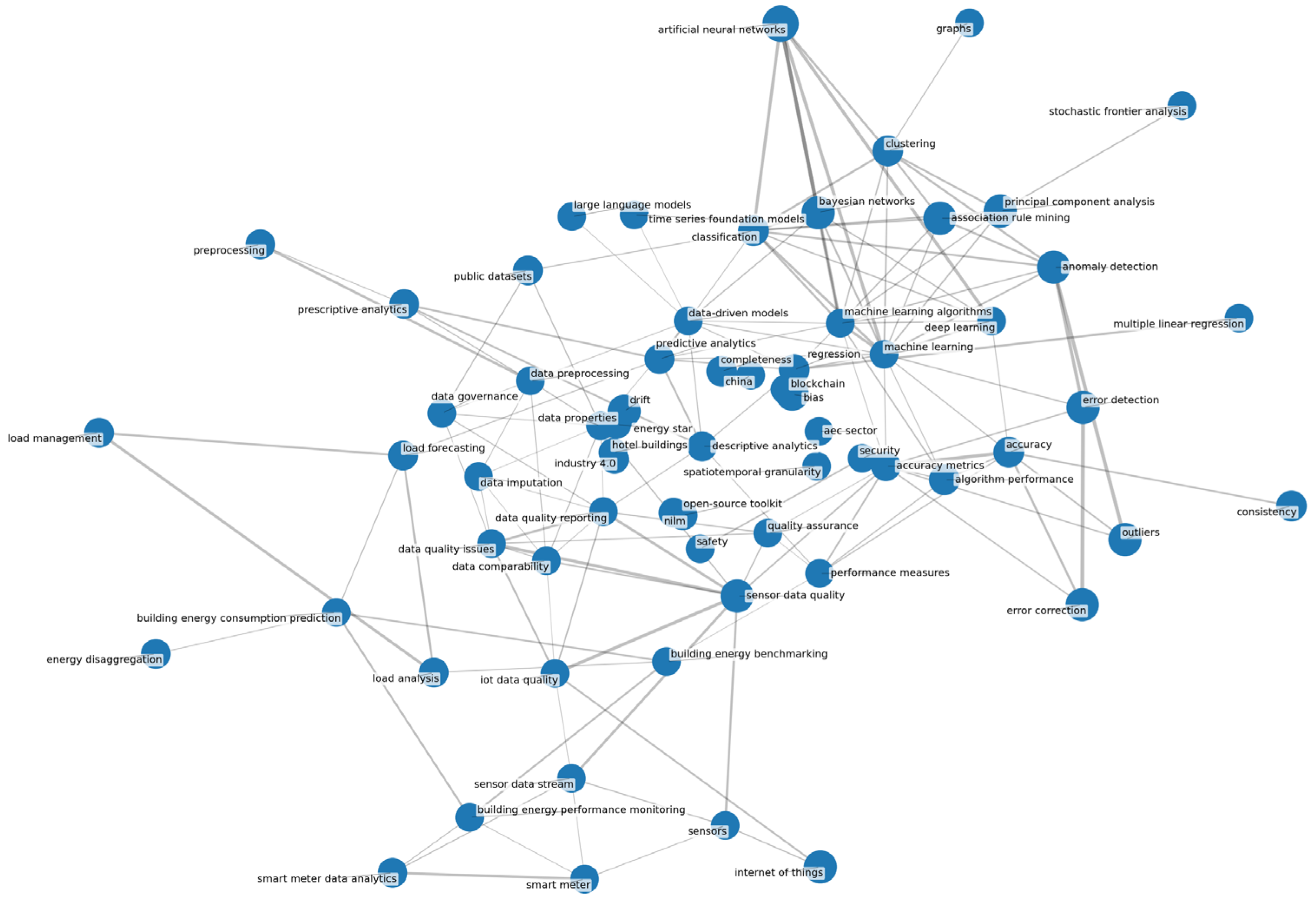
Figure 1. Bibliometric landscape of related works.
Information 16 00836 g001
Figure 2. Overview of the seven-step data quality assurance pipeline, including profiling, metric computation, quality scoring, threshold-based flagging, SHAP analysis, LLM-based explanation, and visual diagnostics.
Information 16 00836 g002
Figure 3. Illustrates the proposed LLM-based data quality assurance pipeline.
Information 16 00836 g003
Figure 4. Prompts for generating data narratives.
Information 16 00836 g004
Figure 5. Prompts for generating reports.
Information 16 00836 g005
Figure 6. Pearson correlation heatmap between data quality metrics (rows; defined in Section 3.2) and model error (NMAE) for each NILM model (columns), computed across buildings. Values range from −1 to +1. Positive indicates higher error with larger metric values; negative indicates lower error with larger metric values.
Information 16 00836 g006
Figure 7. BQS and NMAE for five models. Points are building–resolution pairs. Lines are least squares fits per model.
Information 16 00836 g007
Figure 8. Missing data map for building L06.B01 (1H). Yellow gaps highlight extensive missingness in several key sensors, especially during the early part of the dataset.
Information 16 00836 g008
Figure 9. Outlier boxplot of the main meter in building L10.B01 (1H). The data is clean and stable, with tight interquartile ranges and minimal extreme values. The lower and upper edges of the box represent the first quartile (Q1) and third quartile (Q3), respectively. The orange line indicates the median (Q2). The whiskers extend to the most extreme data points within the range defined by the whisker parameter (typically 1.5 × IQR, where IQR = Q3 − Q1). Data points beyond the whiskers are plotted individually as circles and represent outliers.
Information 16 00836 g009
Figure 10. Outlier boxplot of the temperature-dependent load in L06.B01 (1H). The presence of wide IQRs and multiple outliers indicates high variability and noise. The lower and upper edges of the box represent the first quartile (Q1) and third quartile (Q3), respectively. The orange line indicates the median (Q2). The whiskers extend to the most extreme data points within the range defined by the whisker parameter (typically 1.5 × IQR, where IQR = Q3 − Q1). Data points beyond the whiskers are plotted individually as circles and represent outliers.
Information 16 00836 g010
Figure 11. Seasonal decomposition of the main meter signal in L10.B01 (1H). Clear trend and seasonality patterns reflect stable operational cycles.
Information 16 00836 g011
Figure 12. Seasonal decomposition of the temperature-dependent load in L06.B01 (1H). The signal shows irregular seasonality and high residual noise.
Information 16 00836 g012
Figure 13. Pearson correlation heatmap among main_meter (kW), PV_battery_system (kW), and temperature_dependent (kW) for building L06.B01 at 1-h resolution.
Information 16 00836 g013
Figure 14. SHAP feature importance for the BI-LSTM model. The BI-LSTM model is highly sensitive to missing data rates and temporal inconsistencies, with ‘Missing_Rate’, ‘Abnormal_Timestamps’, and ‘Spike_Rate’ being the most influential features. This aligns closely with the intuition behind the BQS weighting, where missingness and time integrity are prioritized.
Information 16 00836 g014
Figure 15. SHAP summary for the Bayesian model. Similar to BI-LSTM, missing data metrics dominate importance, confirming that classical probabilistic models are also impaired by data gaps and temporal noise.
Information 16 00836 g015
Figure 16. SHAP analysis for the Time–Frequency Mask model. Unlike the other models, prioritizes statistical irregularities such as ‘Spike_Rate’ and ‘Outlier_Proportion’, suggesting a model architecture that is more robust to temporal structure but sensitive to volatility and noise.
Information 16 00836 g016
Figure 17. Cross-correlation heatmap between ‘Temperature_dependent (kW)’ and ‘main_meter (kW)’.
Information 16 00836 g017
Figure 18. LLM interpretation of the cross-correlation heatmap.
Information 16 00836 g018
Figure 19. Pairwise plot of sensor distributions.
Information 16 00836 g019
Figure 20. LLM interpretation of the pairwise plot.
Information 16 00836 g020
Figure 21. LLM-generated report of one example dataset.
Information 16 00836 g021
Table 1. Average normalized mean absolute error (NMAE) of selected models before and after NaN handling.
ModelAvg. NMAE (Before)Avg. NMAE (After)
Bayesian0.820.76
BI-LSTM0.710.64
Time–Frequency Mask0.590.53
Table 2. Comparative summary by theme. The present framework differs from prior strands by unifying task-aligned scoring, surrogate-model attributions via SHAP, and assistive LLM narratives that connect quality diagnostics to expected NILM impact.
Study ThemeTypical MethodologyTypical Results ReportedPrimary ContributionRelation to This WorkImpact on PerformanceImpact on Interpretability
NILM toolkits and benchmarkingStandardized pipelines, shared datasets, reference metrics and baselinesCross-model accuracy on multiple datasets, ablations by sampling and featuresReproducible model evaluation and baselinesQuality diagnostics are applied before benchmarking; BQS predicts sensitivity of models to input defectsCleaner inputs strengthen baselines and reduce varianceLimited to metric definitions and plots; little causal attribution
Data quality and validation for sensor time seriesProfiling gaps, spikes, timestamp integrity, unit checks, dataset curation workflowsDescriptive defect statistics and rule outcomesTaxonomy of defects and practical validation proceduresBQS formalizes quality as task-aligned components and links scores to downstream errorIndirect improvement via defect reduction prior to modelingTypically narrative; no model-agnostic attribution to error
Imputation for energy and sensor dataForward fill, interpolation, seasonal naive, Kalman state-space, KNN multivariateReconstruction error on imputed channels; sometimes task deltasGap-handling strategies with cost–accuracy trade-offsNaN handling used as conservative baseline; protocol defined for broader comparisonsSeasonality-aware or model-based methods preserve structure better for medium gapsMethod specific; rarely tied to model-agnostic explanations
Explainability in time-series modelsSHAP or related feature-attribution on task models or surrogatesGlobal and local importances, case studies of driversInterpretable drivers for model behaviorSHAP on a Random Forest surrogate attributes NILM error to concrete BQS metricsEnables targeted remediation that can reduce errorHigh; direct mapping from metric to error contribution
LLM-assisted analytics and reportingZero-shot prompts to generate short narratives from figures and metadataConcise figure-aligned narratives or triage labelsHuman-readable reporting at scaleLightweight LLM converts diagnostics to short narratives; outputs treated as assistiveIndirect; accelerates triage and iteration on data fixesImproves accessibility and traceability of diagnostics
This work, BQS + SHAP + LLMTask-aligned scoring, surrogate-model attribution, narrative reportingCorrelation between BQS and NILM error, before after-effects for simple NaN handlingUnified pipeline connecting data quality to task performance with interpretable outputsBQS predicts error sensitivity, SHAP identifies dominant defect families, LLM summarizes diagnosticsDemonstrated error reductions under simple remediation; extensible to stronger imputersHigh; model-agnostic linkage from specific defects to expected impact
Table 3. Qualitative comparison of common data cleaning techniques that are appropriate for building sensor data.
MethodPreserves Diurnal or Weekly PatternHandles Long GapsUses Other SensorsTuning BurdenNotes
Forward fill + mean fallbackNoWeakNoNoneConservative baseline, fast, stable for short gaps
Linear interpolationPartial for short gapsWeakNoLowCan oversmooth peaks and transitions
Seasonal naive interpolationYesMediumNoLowHonors seasonal structure if frequency is known
Kalman state-space smoothingYesMediumOptionalMediumCaptures dynamics, requires simple model selection
KNN multivariate imputationPartialMediumYesMediumLeverages correlated channels, sensitive to scaling and k
Disclaimer/Publisher’s Note: The statements, opinions and data contained in all publications are solely those of the individual author(s) and contributor(s) and not of MDPI and/or the editor(s). MDPI and/or the editor(s) disclaim responsibility for any injury to people or property resulting from any ideas, methods, instructions or products referred to in the content.